This work is dedicated to Jim Wilkinson whose ideas and
spirit have given us inspiration and influenced the project
at every turn.
The printed version of LAPACK Users' Guide, Second Edition will be available
from SIAM in February 1995. The list price is $28.50 and the SIAM Member Price
is $22.80.Contact SIAM for additional information.
mail: SIAM, 3600 University City Science Center, Philadelphia, PA 19104-2688.
The royalties from the sales of this book are being placed in a fund
to help students attend SIAM meetings and other SIAM related activities.
This fund is administered by SIAM and qualified individuals are encouraged to
write directly to SIAM for guidelines.
Tue Nov 29 14:03:33 EST 1994
Contents


Next:
List of Tables
Up:
LAPACK Users' Guide Release
Previous:
LAPACK Users' Guide Release
Tue Nov 29 14:03:33 EST 1994
LAPACK Compared with LINPACK and EISPACK

Next:
LAPACK and the
Up:
Essentials
Previous:
Computers for which
LAPACK has been designed to supersede LINPACK
[26]
and EISPACK
[44]
[70]
, principally by restructuring the software to achieve much greater efficiency, where possible, on modern
high-performance computers; also by adding extra functionality,
by using some new or improved algorithms, and
by integrating the two sets
of algorithms into a unified package.
Appendix
D lists the LAPACK counterparts of LINPACK
and EISPACK routines. Not all the facilities of LINPACK and EISPACK are
covered by Release 2.0 of LAPACK.
Tue Nov 29 14:03:33 EST 1994
Design and Documentation of Argument Lists
Next:
Structure of the
Up:
Documentation and Software
Previous:
Documentation and Software
The argument lists of all LAPACK routines conform to a single
set of conventions for their design and documentation.
Specifications of all LAPACK driver and computational routines are given
in Part
2. These are derived from the specifications
given in the leading comments in the code, but in Part
2
the specifications for
real and complex versions of each routine have been merged, in order to
save space.
Tue Nov 29 14:03:33 EST 1994
Structure of the Documentation
Next:
Order of Arguments
Up:
Design and Documentation
Previous:
Design and Documentation
The documentation
of each LAPACK
routine includes:
- the SUBROUTINE or FUNCTION statement, followed by statements
declaring the type and dimensions of the arguments;
- a summary of the Purpose of the routine;
- descriptions of each of the Arguments in the order of
the argument list;
- (optionally) Further Details
(only in the code, not in Part
2);
- (optionally) Internal Parameters
(only in the code, not in Part
2).
Tue Nov 29 14:03:33 EST 1994
Order of Arguments
Next:
Argument Descriptions
Up:
Design and Documentation
Previous:
Structure of the
Arguments
of an LAPACK routine appear
in the following order:
- arguments specifying options;
- problem dimensions;
- array or scalar arguments defining the input data; some of them may be
overwritten by results;
- other array or scalar arguments returning results;
- work arrays (and associated array dimensions);
- diagnostic argument INFO.
Tue Nov 29 14:03:33 EST 1994
Argument Descriptions
Next:
Option Arguments
Up:
Design and Documentation
Previous:
Order of Arguments
The style of the argument
descriptions is illustrated by the following example:
- N
- (input) INTEGER
The number of columns of the matrix A. N > = 0.
- A
- (input/output) REAL array, dimension (LDA,N)
On entry, the m-by-n matrix to be factored.
On exit, the factors L and U from the factorization
A = P * L * U; the unit diagonal elements of L are not stored.
The description of each argument gives:
- a classification of the argument as (input), (output),
(input/output), (input or output)
 ,
(workspace) or (workspace/output)
;
,
(workspace) or (workspace/output)
;
- the type of the argument;
- (for an array) its dimension(s);
- a specification of the value(s) that must be supplied for the
argument (if it's an input argument), or of the value(s) returned
by the routine (if it's an output argument), or both (if it's an
input/output argument). In the last case, the two parts of the
description are introduced by the phrases ``On entry'' and
``On exit''.
- (for a scalar input argument) any constraints that the
supplied values must satisfy (such as ``N > = 0'' in the
example above).
Tue Nov 29 14:03:33 EST 1994
Option Arguments
Next:
Problem Dimensions
Up:
Design and Documentation
Previous:
Argument Descriptions
Arguments
specifying options are
usually of type CHARACTER*1.
The meaning of each valid value is given
, as in this
example:
- UPLO
- (input) CHARACTER*1
= 'U': Upper triangle of A is stored;
= 'L': Lower triangle of A is stored.
The corresponding lower-case characters
may be supplied (with the same meaning), but any other value is illegal
(see subsection
5.1.8).
A longer
character string can be passed as the actual argument, making the calling
program more readable, but only the first character is significant;
this is a standard feature of Fortran 77.
For example:
CALL SPOTRS('upper', . . . )
Tue Nov 29 14:03:33 EST 1994
Problem Dimensions
Next:
Array Arguments
Up:
Design and Documentation
Previous:
Option Arguments
It is permissible for the problem
dimensions
to be passed as zero, in
which case the computation (or part of it) is skipped.
Negative dimensions are regarded as erroneous.
Tue Nov 29 14:03:33 EST 1994
Array Arguments
Next:
Work Arrays
Up:
Design and Documentation
Previous:
Problem Dimensions
Each two-dimensional array argument
is
immediately followed in the
argument list by its leading dimension
, whose
name has the form LD<array-name>. For example:
- A
- (input/output) REAL/COMPLEX array, dimension (LDA,N)
... - LDA
- (input) INTEGER
The leading dimension of the array A. LDA > = max(1,M).
It should be assumed, unless stated otherwise, that vectors and
matrices are stored in one- and two-dimensional arrays in the
conventional manner. That is, if an array X of dimension (N) holds
a vector  , then X(i) holds
  for
for
i = 1,..., n.
If a two-dimensional array A of dimension (LDA,N) holds an m-by-n
matrix A,
then A(i,j) holds  for i = 1,..., m and
j = 1,..., n (LDA must be at least m).
See Section
5.3 for more about
storage of matrices.
for i = 1,..., m and
j = 1,..., n (LDA must be at least m).
See Section
5.3 for more about
storage of matrices.
Note that
array arguments are usually declared in the software as assumed-size arrays
(last dimension *), for example:
REAL A( LDA, * )
although the documentation gives the dimensions as (LDA,N). The latter
form is more informative since it specifies the required minimum value of
the last dimension. However
an assumed-size array declaration has been used in the software,
in order to overcome some
limitations in the Fortran 77 standard. In particular it allows the
routine to be called when the relevant dimension (N, in this case) is zero.
However actual array dimensions in the calling program must be at
least 1 (LDA in this example).
Tue Nov 29 14:03:33 EST 1994
Work Arrays
Next:
Error Handling and
Up:
Design and Documentation
Previous:
Array Arguments
Many LAPACK routines require one or more work
arrays
to be passed as
arguments. The name of a work array is usually WORK - sometimes
IWORK, RWORK or BWORK to distinguish work arrays of
integer, real or logical (Boolean) type.
Occasionally the first element of a work array is used to return some
useful information: in such cases, the argument is described as
(workspace/output) instead of simply (workspace).
A number of routines implementing block algorithms require workspace
sufficient to hold one block of rows or columns of the matrix,
for example, workspace
of size n-by-nb, where nb is the block size.
In such cases, the actual declared length of the work array
must be passed as a separate argument LWORK
,
which immediately follows WORK in the argument-list.
See Section
5.2 for further explanation.
Tue Nov 29 14:03:33 EST 1994
Error Handling and the Diagnostic Argument INFO
Next:
Determining the Block
Up:
Design and Documentation
Previous:
Work Arrays
All
documented routines
have a
diagnostic argument INFO
that
indicates the success or failure of the computation, as follows:
- INFO = 0: successful termination
- INFO < 0: illegal value of one or more arguments - no computation
performed
- INFO > 0: failure in the course of computation
All driver and auxiliary routines
check that input arguments such as N or LDA or
option arguments of type character
have permitted values.
If an illegal value of the i-th argument is detected, the routine
sets INFO = -i, and then calls an error-handling routine XERBLA.
The standard version of XERBLA issues an error message and halts execution,
so that no LAPACK routine would ever return to the calling program with
INFO < 0. However, this might occur if a non-standard version of XERBLA
is used.
Tue Nov 29 14:03:33 EST 1994
Determining the Block Size for Block Algorithms
Next:
Matrix Storage Schemes
Up:
Documentation and Software
Previous:
Error Handling and
LAPACK routines that implement block algorithms need to determine
what block size
to use.
The intention behind the design of LAPACK is that the choice of block size
should be hidden from users as much as possible, but at the same time
easily accessible to installers of the package
when tuning LAPACK for a particular machine.
LAPACK routines call an auxiliary enquiry function ILAENV
, which returns
the optimal block size to be used, as well as other parameters.
The version of ILAENV
supplied with the
package contains
default values that led to good behavior over a reasonable
number of our test machines, but to achieve optimal
performance, it may be beneficial to
tune ILAENV
for your
particular machine environment.
Ideally a distinct implementation of ILAENV is needed for each
machine environment (see also Chapter
6).
The optimal block size may also depend on the routine, the combination of
option arguments (if any), and the problem dimensions.
If ILAENV
returns a block size
of 1, then the routine performs the unblocked algorithm, calling Level 2 BLAS,
and makes no calls to Level 3 BLAS.
Some LAPACK routines require a work array whose size is proportional to
the block size (see subsection
5.1.7). The actual length
of the work array is supplied as an argument LWORK. The description of
the arguments WORK and LWORK typically goes as follows:
- WORK
- (workspace) REAL array, dimension (LWORK)
On exit, if INFO = 0, then WORK(1) returns the optimal LWORK.
- LWORK
- (input) INTEGER
The dimension of the array WORK. LWORK  max(1,N).
For optimal performance LWORK
N*NB,
where NB is the optimal block size returned by ILAENV.
The routine determines the block size to be used by the following steps:
- the optimal block size is determined by calling ILAENV;
- if the value of LWORK indicates that enough workspace has been
supplied, the routine uses the optimal block size;
- otherwise, the routine determines the largest block size that
can be used with the supplied amount of workspace;
- if this new block size does not fall below a
threshold value (also returned by ILAENV), the routine uses the new
value;
- otherwise, the routine uses the unblocked algorithm.
The minimum value of LWORK that would be needed to use
the optimal block size, is returned in WORK(1).
Thus, the routine uses the largest block size allowed by the amount
of workspace supplied, as long as this is likely to
give better performance than the unblocked algorithm.
WORK(1) is not always a simple formula in terms of N and NB.
The specification of LWORK gives the minimum value for the
routine to return correct results. If the supplied value is less than
the minimum - indicating that there is insufficient workspace to perform
the unblocked algorithm - the value of LWORK is regarded as an illegal value,
and is treated like any other illegal argument value
(see subsection
5.1.8).
If in doubt about how much workspace to supply, users should supply a generous
amount (assume a block size of 64, say),
and then examine the value of WORK(1) on exit.
Next:
Matrix Storage Schemes
Up:
Documentation and Software
Previous:
Error Handling and
Tue Nov 29 14:03:33 EST 1994
LAPACK and the BLAS
Next:
Documentation for LAPACK
Up:
Essentials
Previous:
LAPACK Compared with
LAPACK routines are written so that as much as possible of the
computation is performed by calls to the
Basic Linear Algebra Subprograms (BLAS)
[28]
[30]
[58]
.
Highly efficient machine-specific implementations of the BLAS are
available for many modern high-performance computers. The BLAS
enable LAPACK routines to achieve high performance with portable code.
The methodology for
constructing LAPACK routines in terms of calls to the BLAS
is described in Chapter
3.
The BLAS are not strictly speaking part of LAPACK, but Fortran 77 code
for the BLAS is distributed with LAPACK, or can be obtained separately
from netlib (see below). This code constitutes the
``model implementation''
[27]
[29].
The model implementation is not expected
to perform as well as a specially tuned implementation
on most high-performance computers - on some machines it may give much
worse performance - but it
allows users to run LAPACK codes on machines that do not offer any other
implementation of the BLAS.
Tue Nov 29 14:03:33 EST 1994
Matrix Storage Schemes
Next:
Conventional Storage
Up:
Documentation and Software
Previous:
Determining the Block
LAPACK allows the following different storage schemes
for matrices:
- conventional storage in a two-dimensional array;
- packed storage for symmetric, Hermitian or triangular matrices;
- band storage for band matrices;
- the use of two or three
one-dimensional arrays to store tridiagonal or bidiagonal
matrices.
These storage schemes are compatible with those
used in LINPACK
and the BLAS, but EISPACK
uses incompatible schemes
for band and tridiagonal matrices.
In the examples below,  indicates an array element that need not be set
and is not referenced by LAPACK routines. Elements that ``need not be
set'' are never read, written to, or otherwise accessed by the LAPACK
routines. The examples illustrate only the
relevant part of the arrays; array arguments may of course have additional
rows or columns, according to the usual rules for passing array arguments
in Fortran 77.
indicates an array element that need not be set
and is not referenced by LAPACK routines. Elements that ``need not be
set'' are never read, written to, or otherwise accessed by the LAPACK
routines. The examples illustrate only the
relevant part of the arrays; array arguments may of course have additional
rows or columns, according to the usual rules for passing array arguments
in Fortran 77.
Tue Nov 29 14:03:33 EST 1994
Conventional Storage
Next:
Packed Storage
Up:
Matrix Storage Schemes
Previous:
Matrix Storage Schemes
The default scheme for storing matrices
is the obvious one described in subsection
5.1.6:
a matrix A is stored in a two-dimensional array A, with
matrix element
stored in array element A(i,j).
If a matrix is triangular
(upper or lower, as specified by
the argument UPLO), only the elements of the relevant triangle
are accessed. The remaining elements of the array need not be set.
Such elements are indicated by * in the examples below.
For example, when n = 4:

Similarly, if the matrix is upper Hessenberg, elements below the
first subdiagonal need not be set.
Routines that handle symmetric
or Hermitian
matrices
allow for either the upper or lower triangle of the matrix
(as specified by UPLO) to
be stored in the corresponding elements of the array; the remaining
elements of the array need not be set.
For example, when n = 4:

Tue Nov 29 14:03:33 EST 1994
Packed Storage
Next:
Band Storage
Up:
Matrix Storage Schemes
Previous:
Conventional Storage
Symmetric, Hermitian or triangular matrices may be stored more
compactly
, if the relevant
triangle (again as specified by UPLO) is packed
by columns in a one-dimensional array. In LAPACK, arrays that hold
matrices in packed storage, have names ending in `P'. So:
- if UPLO = `U',
is stored in AP(i + j(j - 1)/2) for i < = j;
- if UPLO = `L',
is stored in
AP(i + (2n - j)(j - 1)/2) for
j < = i.
For example:

Note that for real or complex symmetric matrices,
packing the upper triangle
by columns is equivalent to packing the lower triangle by rows;
packing the lower triangle by columns is equivalent to packing
the upper triangle by rows.
For complex Hermitian matrices,
packing the upper triangle
by columns is equivalent to packing the conjugate of the lower triangle by rows;
packing the lower triangle by columns is equivalent to packing
the conjugate of the upper triangle by rows.
Tue Nov 29 14:03:33 EST 1994
Band Storage
Next:
Tridiagonal and Bidiagonal
Up:
Matrix Storage Schemes
Previous:
Packed Storage
An m-by-n band matrix
with kl subdiagonals
and ku superdiagonals may be
stored compactly in a two-dimensional array with kl + ku + 1 rows and n columns.
Columns of the matrix are stored in corresponding columns of the
array, and diagonals of the matrix are stored in rows of the array.
This storage scheme should be used in practice only if kl , ku << min(m , n),
although LAPACK routines work correctly for all values of kl and ku.
In LAPACK, arrays that hold matrices in band storage have names
ending in `B'.
To be precise,
is stored in AB(ku + 1 + i - j , j) for
max(1 , j - ku) < = i < = min(m , j + kl).
For example, when m = n = 5, kl = 2 and ku = 1:

The elements marked * in the upper left and lower right
corners of the array AB need not be set, and are not referenced by
LAPACK routines.
Note: when a band matrix is supplied for LU factorization,
space
must be allowed to store an
additional kl superdiagonals,
generated by fill-in as a result of row interchanges.
This means that the matrix is stored according to the above scheme,
but with kl + ku superdiagonals.
Triangular band matrices are stored in the same format, with either
kl = 0 if upper triangular, or ku = 0 if
lower triangular.
For symmetric or Hermitian band matrices with kd subdiagonals or
superdiagonals, only the upper or lower triangle (as specified by
UPLO) need be stored:
- if UPLO = `U',
is stored in AB(kd + 1 + i - j , j) for
max(1 , j - kd) < = i < = j;
- if UPLO = `L',
is stored in AB(1 + i - j , j) for
j < = i < = min(n , j + kd).
For example, when n = 5 and kd = 2:

EISPACK
routines use a different storage scheme for band matrices,
in which rows of the matrix are stored in corresponding rows of the
array, and diagonals of the matrix are stored in columns of the array
(see Appendix
D).
Tue Nov 29 14:03:33 EST 1994
Tridiagonal and Bidiagonal Matrices
Next:
Unit Triangular Matrices
Up:
Matrix Storage Schemes
Previous:
Band Storage
An unsymmetric
tridiagonal matrix of order n is stored in
three one-dimensional arrays, one of length n containing the
diagonal elements, and two of length n - 1 containing the
subdiagonal and superdiagonal elements in elements 1 : n - 1.
A symmetric
tridiagonal or
bidiagonal
matrix is stored in
two one-dimensional arrays, one of length n containing the
diagonal elements, and one of length n containing the
off-diagonal elements. (EISPACK routines store the off-diagonal
elements in elements 2 : n of a vector of length n.)
Tue Nov 29 14:03:33 EST 1994
Unit Triangular Matrices
Next:
Real Diagonal Elements
Up:
Matrix Storage Schemes
Previous:
Tridiagonal and Bidiagonal
Some LAPACK routines have an option to handle unit triangular matrices
(that is, triangular matrices with diagonal elements = 1). This option
is specified by an argument DIAG
. If DIAG = 'U' (Unit triangular),
the diagonal elements of the matrix need not be stored, and the
corresponding array elements are not referenced by the LAPACK routines.
The storage scheme for the rest of the matrix (whether conventional,
packed or band) remains unchanged, as described in
subsections
5.3.1,
5.3.2 and
5.3.3.
Tue Nov 29 14:03:33 EST 1994
Real Diagonal Elements of Complex Matrices
Next:
Representation of Orthogonal
Up:
Matrix Storage Schemes
Previous:
Unit Triangular Matrices
Complex Hermitian
matrices
have diagonal matrices that are by definition
purely real. In addition, some complex triangular matrices computed by
LAPACK routines are defined by the algorithm to have real diagonal elements
- in Cholesky or QR factorization, for example.
If such matrices are supplied as input to LAPACK routines,
the imaginary parts of the diagonal elements are not referenced,
but are assumed to be zero. If such matrices are returned as output by LAPACK
routines, the computed imaginary parts are explicitly set to zero.
Tue Nov 29 14:03:33 EST 1994
Representation of Orthogonal or Unitary Matrices
Next:
Installing LAPACK Routines
Up:
Documentation and Software
Previous:
Real Diagonal Elements
A real orthogonal or complex unitary matrix (usually denoted Q) is often
represented
in
LAPACK as a product of elementary reflectors - also referred to as
elementary Householder matrices (usually denoted  ). For example,

Most users need not be aware
of the details, because LAPACK routines are provided to work with this
representation:
- routines whose names begin SORG- (real) or CUNG- (complex) can generate
all or part of Q explicitly;
- routines whose name begin SORM- (real) or CUNM- (complex) can multiply
a given matrix by Q or
 without forming Q explicitly.
The following further details may occasionally be useful.
An elementary reflector (or elementary Householder matrix) H of order
n is a
unitary matrix
of the form

where  is a scalar, and v is an n-vector, with
 ); v is often referred to
as the Householder vector
.
Often v has several leading or trailing zero elements, but for the
purpose of this discussion assume that H has no such special structure.
); v is often referred to
as the Householder vector
.
Often v has several leading or trailing zero elements, but for the
purpose of this discussion assume that H has no such special structure.
There is some redundancy in the representation (
5.1), which can be
removed in
various ways. The representation used in LAPACK (which differs from
those used in LINPACK or EISPACK) sets  ; hence
  need not
be stored. In real arithmetic,
need not
be stored. In real arithmetic,  , except that
 implies H = I.
In complex arithmetic
,
may be
complex, and satisfies
 and
and  .
Thus a complex H is
not Hermitian (as it is in other representations), but it is unitary,
which is the important property. The advantage of allowing
to be
complex is that, given an arbitrary complex vector x, H can be computed
so that
.
Thus a complex H is
not Hermitian (as it is in other representations), but it is unitary,
which is the important property. The advantage of allowing
to be
complex is that, given an arbitrary complex vector x, H can be computed
so that

with real  . This is useful, for example,
when reducing a complex Hermitian matrix to real symmetric tridiagonal form
,
or a complex rectangular matrix to real bidiagonal form
.
. This is useful, for example,
when reducing a complex Hermitian matrix to real symmetric tridiagonal form
,
or a complex rectangular matrix to real bidiagonal form
.
For further details, see Lehoucq
[59].
Next:
Installing LAPACK Routines
Up:
Documentation and Software
Previous:
Real Diagonal Elements
Tue Nov 29 14:03:33 EST 1994
Installing LAPACK Routines
Next:
Points to Note
Up:
Guide
Previous:
Representation of Orthogonal
Tue Nov 29 14:03:33 EST 1994
Points to Note
Next:
Installing ILAENV
Up:
Installing LAPACK Routines
Previous:
Installing LAPACK Routines
For anyone who obtains the complete LAPACK package from netlib
or NAG (see Chapter
1), a
comprehensive installation
guide
is provided. We recommend
installation of the complete package as the most convenient and reliable
way to make LAPACK available.
People who obtain copies of a few LAPACK routines from netlib need to be
aware of the following points:
- Double precision complex routines (names beginning Z-)
use a COMPLEX*16 data type. This is an extension to the Fortran 77
standard, but is provided by many Fortran compilers on machines
where double precision computation is usual.
The following related extensions are also used:
- the intrinsic function DCONJG, with argument and result of type
COMPLEX*16;
- the intrinsic functions DBLE and DIMAG, with COMPLEX*16 argument
and DOUBLE PRECISION result, returning the real and imaginary parts,
respectively;
- the intrinsic function DCMPLX, with DOUBLE PRECISION argument(s)
and COMPLEX*16 result;
- COMPLEX*16 constants, formed from a pair of double precision
constants in parentheses.
Some compilers provide DOUBLE COMPLEX as an alternative to COMPLEX*16,
and an intrinsic function DREAL instead of DBLE to return the
real part of a COMPLEX*16 argument.
If the compiler does not accept the constructs used in LAPACK, the installer
will have to modify the code: for example, globally change COMPLEX*16 to
DOUBLE COMPLEX, or selectively change DBLE to DREAL.
-
For optimal performance, a small set of tuning parameters must be set
for each machine, or even for each configuration of a given machine
(for example, different parameters may be optimal for different numbers
of processors).
These values
, such as the block size, minimum block size, crossover
point below which an unblocked routine should be used, and others,
are set by calls to an inquiry function ILAENV.
The default version of ILAENV
provided with LAPACK uses generic values
which often give satisfactory performance, but
users who are particularly interested in performance may wish to
modify this subprogram or substitute their own version.
Further details on setting ILAENV for a particular environment
are provided in section
6.2.
-
SLAMCH/DLAMCH
determines properties of the
floating-point arithmetic at run-time, such as the machine epsilon,
underflow threshold,
overflow threshold, and related parameters. It works satisfactorily on
all commercially important machines of which we are aware, but will necessarily
be updated from time to time as new machines and compilers are produced.
Next:
Installing ILAENV
Up:
Installing LAPACK Routines
Previous:
Installing LAPACK Routines
Tue Nov 29 14:03:33 EST 1994
Documentation for LAPACK
Next:
Availability of LAPACK
Up:
Essentials
Previous:
LAPACK and the
This Users' Guide gives an informal introduction to
the design of the package, and a detailed description of its contents.
Chapter
5 explains the conventions used in the
software and documentation.
Part
2 contains complete specifications of all the
driver routines and computational routines. These specifications have been
derived from the leading comments in the source text.
On-line manpages (troff files) for LAPACK routines, as well as for most of
the BLAS routines, are available on netlib. These files are
automatically generated at the time of each release. For more
information, see the manpages.tar.z entry on the lapack
index on netlib.
Tue Nov 29 14:03:33 EST 1994
Installing ILAENV
Next:
Troubleshooting
Up:
Installing LAPACK Routines
Previous:
Points to Note
Machine-dependent
parameters
such as the block size are set
by calls to an inquiry function which may be set with different
values on each machine.
The declaration of the environment inquiry function is
INTEGER FUNCTION ILAENV( ISPEC, NAME, OPTS, N1, N2, N3, N4 )
where ISPEC, N1, N2, N3, and N4 are integer variables and
NAME and OPTS are CHARACTER*(*). NAME specifies the subroutine name:
OPTS is a character string of options to the subroutine; and N1-N4 are
the problem dimensions.
ISPEC specifies the parameter to be returned; the following values are
currently used in LAPACK:
ISPEC = 1: NB, optimal block size
= 2: NBMIN, minimum block size for the block routine
to be used
= 3: NX, crossover point (in a block routine, for
N < NX, an un blocked routine should be used)
= 4: NS, number of shifts
= 6: NXSVD is the threshold point for which the QR
factorization is performed prior to reduction to
bidiagonal form. If M > NXSVD * N, then a
QR factorization is performed.
= 8: MAXB, crossover point for block multishift QR
The three block size parameters, NB, NBMIN, and NX, are used in many
different
subroutines (see Table
6.1).
NS and MAXB are used
in the
block multishift QR algorithm, xHSEQR.
NXSVD is used
in the driver
routines xGELSS and xGESVD.

Table 6.1: Use of the block parameters NB, NBMIN, and NX in LAPACK
The LAPACK testing and timing programs use a special version of ILAENV
where the parameters are set via a COMMON block interface.
This is convenient for experimenting with different values of, say,
the block size in order to exercise different parts of the code
and to compare the relative performance of different parameter values.
The LAPACK timing programs were designed to collect data for all the
routines in Table
6.1.
The range of problem sizes needed to determine the optimal block size
or crossover point
is machine-dependent, but the
input files
provided with the LAPACK test and timing package can be used as a
starting point.
For subroutines that require a crossover point, it is best to start by
finding the best block size
with the crossover
point set to 0, and then
to locate the point at which the performance of the unblocked algorithm
is beaten by the block algorithm.
The best crossover point
will be somewhat smaller than the point
where the curves for the unblocked and blocked methods cross.
For example, for SGEQRF
on a single processor of a CRAY-2,
NB = 32 was observed to be a good block size
,
and the performance of the block algorithm with this block size
surpasses the unblocked algorithm for square matrices
between N = 176 and N = 192.
Experiments with crossover points from 64 to 192 found that NX = 128
was a good choice, although the results for NX from 3*NB to 5*NB
are broadly similar.
This means that matrices with N < = 128 should use the unblocked
algorithm, and for N > 128 block updates should be used until the
remaining submatrix has order less than 128.
The performance of the unblocked (NB = 1) and blocked (NB = 32)
algorithms for SGEQRF
and for the blocked algorithm with a crossover
point of 128 are compared in Figure
6.1.

Figure 6.1: QR factorization on CRAY-2 (1 processor)
By experimenting with small values of the block size,
it should be straightforward to choose NBMIN,
the smallest block size that gives a performance improvement
over the unblocked algorithm.
Note that on some machines, the optimal block size may be 1
(the unblocked algorithm gives the best performance);
in this case, the choice of NBMIN is arbitrary.
The prototype version of ILAENV
sets NBMIN to 2, so that blocking
is always done, even though this could lead to poor performance
from a block routine if insufficient workspace is supplied
(see chapter
7).
Complicating the determination of optimal parameters is the fact that
the orthogonal factorization routines and SGEBRD
accept non-square
matrices as input.
The LAPACK timing program allows M and N to be varied independently.
We have found the optimal block size to be
generally insensitive to the shape of the matrix,
but the crossover point is more dependent on the matrix shape.
For example, if
M >> N in the QR factorization, block updates
may always be faster than unblocked updates on the remaining submatrix,
so one might set NX = NB if M > = 2N.
Parameter values for the number of shifts, etc.
used to tune the block multishift QR
algorithm
can be varied from the input files to the eigenvalue timing program.
In particular, the performance of xHSEQR is particularly sensitive to
the correct choice of block parameters. Setting NS = 2 will give
essentially the same performance as EISPACK
.
Interested users should consult
[3] for a description of
the timing program input files.
Next:
Troubleshooting
Up:
Installing LAPACK Routines
Previous:
Points to Note
Tue Nov 29 14:03:33 EST 1994
Troubleshooting
Next:
Common Errors in
Up:
Guide
Previous:
Installing ILAENV
Tue Nov 29 14:03:33 EST 1994
Common Errors in Calling LAPACK Routines
Next:
Failures Detected by
Up:
Troubleshooting
Previous:
Troubleshooting
For the benefit of less experienced programmers, we give here a list of
common programming errors in calling an LAPACK routine.
These errors may cause the LAPACK routine to report a failure,
as described in Section
7.2
;
they may cause an error to be reported by the system;
or they may lead to wrong results - see also
Section
7.3.
- wrong number of arguments
- arguments in the wrong order
- an argument of the wrong type (especially real and complex
arguments of the wrong precision)
- wrong dimensions for an array argument
- insufficient space in a workspace argument
- failure to assign a value to an input argument
Some modern compilation systems, as well as
software tools such as the portability checker in
Toolpack
[66], can check that arguments agree in number and type;
and many compilation systems offer run-time detection
of errors such as an array element out-of-bounds or use of an
unassigned variable.
Tue Nov 29 14:03:33 EST 1994
Failures Detected by LAPACK Routines
Next:
Invalid Arguments and
Up:
Troubleshooting
Previous:
Common Errors in
There are two ways in which an LAPACK routine may report a failure to
complete a computation successfully.
Tue Nov 29 14:03:33 EST 1994
Invalid Arguments and XERBLA
Next:
Computational Failures and
Up:
Failures Detected by
Previous:
Failures Detected by
If an illegal value is supplied for one of the input arguments to
an LAPACK routine, it will call the error handler XERBLA to write
a message to the standard output unit of the form:
** On entry to SGESV parameter number 4 had an illegal value
This particular message would be caused by passing to SGESV
a value of LDA
which was less than the value of the argument N.
The documentation for SGESV
in Part
2 states the set of acceptable input values:
``LDA > = max(1,N).'' This is required in order that the
array A with leading dimension LDA can store an n-by-n
matrix.
The arguments are checked in order, beginning with the first.
In the above example, it may - from the user's point of view - be the
value of N which is in fact wrong.
Invalid arguments are often caused by the kind of error listed in
Section
7.1.
In the model implementation of XERBLA
which is supplied with LAPACK,
execution stops after the
message; but the call to XERBLA is followed by a RETURN statement
in the LAPACK routine, so that if the installer removes the
STOP statement in XERBLA, the result will be an immediate exit from the
LAPACK routine with a negative value of INFO.
It is good practice always to check for a non-zero value of INFO
on return from an LAPACK routine.
(We recommend however that XERBLA should not be modified to return control
to the calling routine, unless absolutely
necessary, since this would remove one of the built-in safety-features
of LAPACK.)
Tue Nov 29 14:03:33 EST 1994
Computational Failures and INFO > 0
Next:
Wrong Results
Up:
Failures Detected by
Previous:
Invalid Arguments and
A positive value of INFO on return from an LAPACK routine indicates a
failure in the course of the algorithm. Common causes are:
- a matrix is singular (to working precision);
- a symmetric matrix is not positive definite;
- an iterative algorithm for computing eigenvalues or eigenvectors
fails to converge in the permitted number of iterations.
For example, if SGESVX
is called to solve a system of equations
with a coefficient matrix that is approximately singular,
it may detect exact singularity at the i-th stage of the LU
factorization, in which case it returns INFO = i;
or (more probably) it may compute an estimate of the reciprocal condition number
that is less than machine precision, in which case it returns INFO = n + 1.
Again, the documentation in Part
2 should be consulted for a
description of the error.
When a failure with INFO > 0 occurs, control is always returned
to the calling program; XERBLA is not called, and no error message
is written.
It is worth repeating that it is good practice always to check for
a non-zero value of INFO on return from an LAPACK routine.
A failure with INFO > 0 may indicate any of the following:
- an inappropriate routine was used:
for example, if a routine fails because a symmetric matrix turns out not to be
positive definite, consider using a routine for symmetric indefinite matrices.
- a single precision routine was used when double precision was needed:
for example, if SGESVX
reports approximate singularity
(as illustrated above), the corresponding double precision routine DGESVX
may be able to solve the problem (but nevertheless the problem is
ill-conditioned).
- a programming error occurred in generating the data supplied
to a routine: for example, even though theoretically a matrix should be
well-conditioned and positive-definite, a programming error in generating
the matrix could easily destroy either of those properties.
- a programming error occurred in calling the routine, of the kind
listed in Section
7.1.
Next:
Wrong Results
Up:
Failures Detected by
Previous:
Invalid Arguments and
Tue Nov 29 14:03:33 EST 1994
Wrong Results
Next:
Poor Performance
Up:
Troubleshooting
Previous:
Computational Failures and
Wrong results from LAPACK routines are most often caused by incorrect usage.
It is also possible that wrong results are caused by a bug
outside of LAPACK, in the compiler or in one of the library routines,
such as the BLAS, that are linked with LAPACK.
Test procedures are available for both LAPACK and the BLAS, and
the LAPACK installation guide
[3] should be consulted
for descriptions of the tests and for advice on resolving problems.
A list of known problems, compiler errors, and bugs in LAPACK routines is
maintained on netlib; see Chapter
1.
Users who suspect they have found a new bug in an LAPACK routine are
encouraged to report it promptly to the developers as directed in
Chapter
1.
The bug report should include a test case, a description of
the problem and expected results, and the actions, if any,
that the user has already taken to fix the bug.
Tue Nov 29 14:03:33 EST 1994
Poor Performance
Next:
Index of Driver
Up:
Troubleshooting
Previous:
Wrong Results
We have tried to make
the performance of LAPACK ``transportable'' by performing most of
the computation within the Level 1, 2, and 3 BLAS, and by isolating
all of the machine-dependent tuning parameters
in a single integer function ILAENV
.
To avoid poor performance
from LAPACK
routines, note the
following recommendations
:
- BLAS:
-
One should use BLAS that have been optimized for the machine being used
if they are available.
Many manufacturers and research institutions have developed, or are
developing, efficient versions of the BLAS for particular machines.
A portable set of Fortran BLAS is supplied with LAPACK
and can always be used if no other BLAS are available or if
there is a suspected problem in the local BLAS library, but
no attempt has been made to structure the Fortran BLAS for
high performance.
- ILAENV:
- For best performance, the LAPACK routine ILAENV
should be set with optimal tuning parameters for the machine being used.
The version of ILAENV provided with LAPACK supplies default values
for these parameters that give good, but not optimal, average
case performance on a range of existing machines.
In particular, the performance of xHSEQR is particularly sensitive to
the correct choice of block parameters; the same applies to the driver
routines which call xHSEQR, namely xGEES, xGEESX, xGEEV and xGEEVX.
Further details on setting parameters in ILAENV are found in
section
6.
- LWORK
WORK(1):
-
The performance of some routines depends on the amount of workspace
supplied. In such cases,
an argument, usually called WORK, is
provided, accompanied by an integer argument LWORK specifying its
length as a linear array.
On exit, WORK(1) returns the amount of workspace required to use
the optimal tuning parameters.
If LWORK < WORK(1), then insufficient workspace was provided
to use the optimal parameters, and the performance may be less
than possible.
One should check that LWORK
WORK(1) on return from
an LAPACK routine requiring user-supplied workspace to see if
enough workspace has been provided.
Note that the computation is performed correctly, even if the amount of
workspace is less than optimal, unless LWORK is reported as an
invalid value by a call to XERBLA as described in Section
7.2.
- xLAMCH:
- Users should beware of the high cost of the first
call to the LAPACK auxiliary routine xLAMCH,
which computes
machine characteristics such as epsilon and the
smallest invertible number.
The first call dynamically determines a set of parameters defining
the machine's arithmetic, but these values are saved and subsequent
calls incur only a trivial cost.
For performance testing, the initial cost can be hidden by
including a call to xLAMCH in the main program, before any calls to
LAPACK routines that will be timed. A sample use of SLAMCH
is
XXXXXX = SLAMCH( 'P' )
or in double precision:
XXXXXX = DLAMCH( 'P' )
A cleaner but less portable solution is for the installer to
save the values computed by xLAMCH for a specific machine
and create a new version of xLAMCH with these constants set in
DATA statements, taking care that no accuracy is lost in the
translation.
Next:
Index of Driver
Up:
Troubleshooting
Previous:
Wrong Results
Tue Nov 29 14:03:33 EST 1994
Index of Driver and Computational Routines
Next:
Notes
Up:
Guide
Previous:
Poor Performance
Tue Nov 29 14:03:33 EST 1994
Notes
Next:
Index of Auxiliary
Up:
Index of Driver
Previous:
Index of Driver
- This index
lists related pairs of real and complex routines together,
for example, SBDSQR and CBDSQR.
- Driver routines are listed in bold type, for example SGBSV and
CGBSV.
- Routines are listed in alphanumeric order
of the real (single precision) routine name (which always begins with S-).
(See subsection
2.1.3 for details of the LAPACK naming scheme.)
- Double precision routines are not listed here;
they have names beginning with D- instead of
S-, or Z- instead of C-.
- This index gives only a brief description of the purpose of each
routine. For a precise description, consult the specifications
in Part
2, where the routines appear in the same
order as here.
- The text of the descriptions applies to both real and complex routines,
except where alternative words or phrases are indicated, for example
``symmetric/Hermitian'', ``orthogonal/unitary''
or ``quasi-triangular/triangular''. For the real routines
 is equivalent
to
is equivalent
to  .
(The same convention is used in Part
2.)
.
(The same convention is used in Part
2.)
- In a few cases, three routines are listed together, one for
real symmetric, one for complex symmetric, and one for complex Hermitian
matrices (for example SSPCON, CSPCON and CHPCON).
- A few routines for real matrices have no complex equivalent (for example
SSTEBZ).


Tue Nov 29 14:03:33 EST 1994
Availability of LAPACK
Next:
Installation of LAPACK
Up:
Essentials
Previous:
Documentation for LAPACK
The complete LAPACK package or individual routines from
LAPACK
are most easily obtained through
netlib
[32]
.
At the time of this writing, the e-mail addresses for netlib are
netlib@ornl.gov
netlib@research.att.com
Both repositories provide electronic mail and anonymous ftp service (the
netlib@ornl.gov cite is available via anonymous ftp to
netlib2.cs.utk.edu), and the
netlib@ornl.gov cite additionally provides xnetlib
. Xnetlib uses an X
Windows graphical user interface and a socket-based connection between
the user's machine and the xnetlib server machine to process software
requests. For more information on xnetlib, echo ``send index from
xnetlib'' | mail netlib@ornl.gov.
General information about LAPACK can be obtained by sending mail to one
of the above addresses with the message
send index from lapack
The package is also available on the World Wide Web. It can be accessed
through the URL address:
http://www.netlib.org/lapack/index.html
The complete package, including test code and timing programs in four
different Fortran data types, constitutes some 735,000 lines of Fortran
source and comments.
Alternatively, if a user does not have internet access, the complete
package can be obtained on magnetic media
from NAG for a cost-covering handling charge.
For further details contact NAG
at one of the following addresses:
NAG Inc. NAG Ltd.
1400 Opus Place, Suite 200 Wilkinson House
Downers Grove, IL 60515-5702 Jordan Hill Road
USA Oxford OX2 8DR
Tel: +1 708 971 2337 England
Fax: +1 708 971 2706 Tel: +44 865 511245
Fax: +44 865 310139
NAG GmbH
Schleissheimerstrasse 5
W-8046 Garching bei Munchen
Germany
Tel: +49 89 3207395
Fax: +49 89 3207396
Tue Nov 29 14:03:33 EST 1994
Index of Auxiliary Routines
Next:
Notes
Up:
Guide
Previous:
Notes
Tue Nov 29 14:03:33 EST 1994
Notes
Next:
Quick Reference
Guide
Up:
Index of Auxiliary
Previous:
Index of Auxiliary
- This index
lists related pairs of real and complex routines together,
in the same style as in Appendix A.
- Routines are listed in alphanumeric order
of the real (single precision) routine name (which always begins with S-).
(See subsection
2.1.3 for details of the LAPACK naming scheme.)
- A few complex routines have no real equivalents, and they are listed
first; routines listed in italics (for example, CROT), have real
equivalents in the Level 1 or Level 2 BLAS.
- Double precision routines are not listed here;
they have names beginning with D- instead of
S-, or Z- instead of C-.
The only exceptions to this simple rule are that
the double precision versions of ICMAX1, SCSUM1 and CSRSCL
are named IZMAX1, DZSUM1 and ZDRSCL.
- A few routines in the list have names that are independent of data type:
ILAENV, LSAME, LSAMEN and XERBLA.
- This index gives only a brief description of the purpose of each
routine. For a precise description consult the leading comments in the code,
which have been written in the same style as for the driver and
computational routines.


Tue Nov 29 14:03:33 EST 1994
Quick Reference<A NAME=7491>
</A>
Guide to the BLAS
Next:
Converting from LINPACK
Up:
Guide
Previous:
Notes
Level 1 BLAS
dim scalar vector vector scalars 5-element prefixes
array
SUBROUTINE _ROTG ( A, B, C, S ) S, D
SUBROUTINE _ROTMG( D1, D2, A, B, PARAM ) S, D
SUBROUTINE _ROT ( N, X, INCX, Y, INCY, C, S ) S, D
SUBROUTINE _ROTM ( N, X, INCX, Y, INCY, PARAM ) S, D
SUBROUTINE _SWAP ( N, X, INCX, Y, INCY ) S, D, C, Z
SUBROUTINE _SCAL ( N, ALPHA, X, INCX ) S, D, C, Z, CS, ZD
SUBROUTINE _COPY ( N, X, INCX, Y, INCY ) S, D, C, Z
SUBROUTINE _AXPY ( N, ALPHA, X, INCX, Y, INCY ) S, D, C, Z
FUNCTION _DOT ( N, X, INCX, Y, INCY ) S, D, DS
FUNCTION _DOTU ( N, X, INCX, Y, INCY ) C, Z
FUNCTION _DOTC ( N, X, INCX, Y, INCY ) C, Z
FUNCTION __DOT ( N, ALPHA, X, INCX, Y, INCY ) SDS
FUNCTION _NRM2 ( N, X, INCX ) S, D, SC, DZ
FUNCTION _ASUM ( N, X, INCX ) S, D, SC, DZ
FUNCTION I_AMAX( N, X, INCX ) S, D, C, Z

Level 2 BLAS
options dim b-width scalar matrix vector scalar vector prefixes
_GEMV ( TRANS, M, N, ALPHA, A, LDA, X, INCX, BETA, Y, INCY ) S, D, C, Z
_GBMV ( TRANS, M, N, KL, KU, ALPHA, A, LDA, X, INCX, BETA, Y, INCY ) S, D, C, Z
_HEMV ( UPLO, N, ALPHA, A, LDA, X, INCX, BETA, Y, INCY ) C, Z
_HBMV ( UPLO, N, K, ALPHA, A, LDA, X, INCX, BETA, Y, INCY ) C, Z
_HPMV ( UPLO, N, ALPHA, AP, X, INCX, BETA, Y, INCY ) C, Z
_SYMV ( UPLO, N, ALPHA, A, LDA, X, INCX, BETA, Y, INCY ) S, D
_SBMV ( UPLO, N, K, ALPHA, A, LDA, X, INCX, BETA, Y, INCY ) S, D
_SPMV ( UPLO, N, ALPHA, AP, X, INCX, BETA, Y, INCY ) S, D
_TRMV ( UPLO, TRANS, DIAG, N, A, LDA, X, INCX ) S, D, C, Z
_TBMV ( UPLO, TRANS, DIAG, N, K, A, LDA, X, INCX ) S, D, C, Z
_TPMV ( UPLO, TRANS, DIAG, N, AP, X, INCX ) S, D, C, Z
_TRSV ( UPLO, TRANS, DIAG, N, A, LDA, X, INCX ) S, D, C, Z
_TBSV ( UPLO, TRANS, DIAG, N, K, A, LDA, X, INCX ) S, D, C, Z
_TPSV ( UPLO, TRANS, DIAG, N, AP, X, INCX ) S, D, C, Z
options dim scalar vector vector matrix prefixes
_GER ( M, N, ALPHA, X, INCX, Y, INCY, A, LDA ) S, D
_GERU ( M, N, ALPHA, X, INCX, Y, INCY, A, LDA ) C, Z
_GERC ( M, N, ALPHA, X, INCX, Y, INCY, A, LDA ) C, Z
_HER ( UPLO, N, ALPHA, X, INCX, A, LDA ) C, Z
_HPR ( UPLO, N, ALPHA, X, INCX, AP ) C, Z
_HER2 ( UPLO, N, ALPHA, X, INCX, Y, INCY, A, LDA ) C, Z
_HPR2 ( UPLO, N, ALPHA, X, INCX, Y, INCY, AP ) C, Z
_SYR ( UPLO, N, ALPHA, X, INCX, A, LDA ) S, D
_SPR ( UPLO, N, ALPHA, X, INCX, AP ) S, D
_SYR2 ( UPLO, N, ALPHA, X, INCX, Y, INCY, A, LDA ) S, D
_SPR2 ( UPLO, N, ALPHA, X, INCX, Y, INCY, AP ) S, D
Level 3 BLAS
options dim scalar matrix matrix scalar matrix prefixes
_GEMM ( TRANSA, TRANSB, M, N, K, ALPHA, A, LDA, B, LDB, BETA, C, LDC ) S, D, C, Z
_SYMM ( SIDE, UPLO, M, N, ALPHA, A, LDA, B, LDB, BETA, C, LDC ) S, D, C, Z
_HEMM ( SIDE, UPLO, M, N, ALPHA, A, LDA, B, LDB, BETA, C, LDC ) C, Z
_SYRK ( UPLO, TRANS, N, K, ALPHA, A, LDA, BETA, C, LDC ) S, D, C, Z
_HERK ( UPLO, TRANS, N, K, ALPHA, A, LDA, BETA, C, LDC ) C, Z
_SYR2K( UPLO, TRANS, N, K, ALPHA, A, LDA, B, LDB, BETA, C, LDC ) S, D, C, Z
_HER2K( UPLO, TRANS, N, K, ALPHA, A, LDA, B, LDB, BETA, C, LDC ) C, Z
_TRMM ( SIDE, UPLO, TRANSA, DIAG, M, N, ALPHA, A, LDA, B, LDB ) S, D, C, Z
_TRSM ( SIDE, UPLO, TRANSA, DIAG, M, N, ALPHA, A, LDA, B, LDB ) S, D, C, Z


Notes
Meaning of prefixes
S - REAL C - COMPLEX
D - DOUBLE PRECISION Z - COMPLEX*16 (this may not be
supported by all
machines)
For the Level 2 BLAS a set of extended-precision routines with the prefixes
ES, ED, EC, EZ may also be available.
Level 1 BLAS
In addition to the listed routines there are two further
extended-precision dot product routines DQDOTI and DQDOTA.
Level 2 and Level 3 BLAS
Matrix types
GE - GEneral GB - General Band
SY - SYmmetric SB - Symmetric Band SP - Symmetric Packed
HE - HErmitian HB - Hermitian Band HP - Hermitian Packed
TR - TRiangular TB - Triangular Band TP - Triangular Packed
Options
Arguments describing options are declared as CHARACTER*1 and may be passed as character strings.
TRANS = 'No transpose', 'Transpose', 'Conjugate transpose' (X, X^T, X^C)
UPLO = 'Upper triangular', 'Lower triangular'
DIAG = 'Non-unit triangular', 'Unit triangular'
SIDE = 'Left', 'Right' (A or op(A) on the left, or A or op(A) on the right)
For real matrices, TRANS = `T' and TRANS = `C' have the same meaning.
For Hermitian matrices, TRANS = `T' is not allowed.
For complex symmetric matrices, TRANS = `H' is not allowed.
Tue Nov 29 14:03:33 EST 1994
Converting from LINPACK or EISPACK
Next:
Notes
Up:
Guide
Previous:
Quick Reference
Guide
This appendix
is designed to assist people to convert programs
that currently call LINPACK or EISPACK routines, to call LAPACK
routines instead.
Tue Nov 29 14:03:33 EST 1994
Notes
Next:
LAPACK Working Notes
Up:
Converting from LINPACK
Previous:
Converting from LINPACK
- The appendix consists mainly of indexes
giving the nearest LAPACK equivalents of LINPACK and EISPACK routines.
These indexes should not be followed blindly or rigidly,
especially when two or more
LINPACK or EISPACK routines are being used together: in many such cases
one of the LAPACK driver routines may be a suitable replacement.
- When two or more LAPACK routines are given in a single entry, these
routines must be combined to achieve the equivalent function.
- For LINPACK, an index is given for equivalents of the real LINPACK
routines; these equivalences apply also to the corresponding complex routines.
A separate table is included for equivalences of complex Hermitian routines.
For EISPACK, an index is given for all real and complex routines,
since there is no direct 1-to-1 correspondence between real and complex
routines in EISPACK.
- A few of the less commonly used routines in LINPACK and EISPACK have no
equivalents in Release 1.0 of LAPACK; equivalents for some of these (but not
all) are planned for a future release.
- For some EISPACK routines, there are LAPACK routines providing similar
functionality, but using a significantly different method, or LAPACK routines
which provide only part of the functionality; such routines are marked by
a
 . For example, the EISPACK routine ELMHES uses non-orthogonal
transformations, whereas the nearest equivalent LAPACK routine, SGEHRD, uses
orthogonal transformations.
. For example, the EISPACK routine ELMHES uses non-orthogonal
transformations, whereas the nearest equivalent LAPACK routine, SGEHRD, uses
orthogonal transformations.
- In some cases the LAPACK equivalents require matrices to be stored
in a different storage scheme. For example:
- EISPACK routines BANDR
, BANDV
,
BQR
and the driver routine RSB
require the lower triangle of
a symmetric band matrix to be stored in
a different storage scheme to that used in LAPACK, which is illustrated in
subsection
5.3.3. The corresponding storage scheme used by the
EISPACK routines is:

- EISPACK routines TRED1
, TRED2
,
TRED3
, HTRID3
,
HTRIDI
, TQL1
,
TQL2
, IMTQL1
,
IMTQL2
, RATQR
,
TQLRAT
and the driver routine RST
store the off-diagonal elements of a symmetric tridiagonal
matrix in elements 2 : n of the array E, whereas LAPACK routines use
elements 1 : n - 1.
- The EISPACK and LINPACK routines for the singular value decomposition
return the matrix of right singular vectors, V, whereas the corresponding
LAPACK routines return the transposed matrix
 .
.
- In general, the argument lists of the
LAPACK routines are different from those of
the corresponding EISPACK and LINPACK
routines, and the workspace requirements are often different.

LAPACK equivalents of LINPACK routines for real matrices
----------------------------------------------------------------
LINPACK LAPACK Function of LINPACK routine
----------------------------------------------------------------
SCHDC Cholesky factorization with diagonal pivoting
option
----------------------------------------------------------------
SCHDD rank-1 downdate of a Cholesky factorization
or the triangular factor of a QR factorization
----------------------------------------------------------------
SCHEX rank-1 update of a Cholesky factorization
or the triangular factor of a QR factorization
----------------------------------------------------------------
SCHUD modifies a Cholesky factorization under
permutations of the original matrix
----------------------------------------------------------------
SGBCO SLANGB LU factorization and condition estimation
SGBTRF of a general band matrix
SGBCON
----------------------------------------------------------------
SGBDI determinant of a general band matrix,
after factorization by SGBCO or SGBFA
----------------------------------------------------------------
SGBFA SGBTRF LU factorization of a general band matrix
----------------------------------------------------------------
SGBSL SGBTRS solves a general band system of linear
equations, after factorization by SGBCO
or SGBFA
----------------------------------------------------------------
SGECO SLANGE LU factorization and condition
SGETRF estimation of a general matrix
SGECON
----------------------------------------------------------------
SGEDI SGETRI determinant and inverse of a general
matrix, after factorization by SGECO
or SGEFA
----------------------------------------------------------------
SGEFA SGETRF LU factorization of a general matrix
----------------------------------------------------------------
SGESL SGETRS solves a general system of linear
equations, after factorization by
SGECO or SGEFA
----------------------------------------------------------------
SGTSL SGTSV solves a general tridiagonal system
of linear equations
----------------------------------------------------------------
SPBCO SLANSB Cholesky factorization and condition
SPBTRF estimation of a symmetric positive definite
SPBCON band matrix
----------------------------------------------------------------
SPBDI determinant of a symmetric positive
definite band matrix, after factorization
by SPBCO or SPBFA
----------------------------------------------------------------
SPBFA SPBTRF Cholesky factorization of a symmetric
positive definite band matrix
----------------------------------------------------------------
SPBSL SPBTRS solves a symmetric positive definite band
system of linear equations, after
factorization by SPBCO or SPBFA
----------------------------------------------------------------
SPOCO SLANSY Cholesky factorization and condition
SPOTRF estimation of a symmetric positive definite
SPOCON matrix
----------------------------------------------------------------
SPODI SPOTRI determinant and inverse of a symmetric
positive definite matrix, after factorization
by SPOCO or SPOFA
----------------------------------------------------------------
SPOFA SPOTRF Cholesky factorization of a symmetric
positive definite matrix
----------------------------------------------------------------
SPOSL SPOTRS solves a symmetric positive definite system
of linear equations, after factorization by
SPOCO or SPOFA
----------------------------------------------------------------
SPPCO SLANSY Cholesky factorization and condition
SPPTRF estimation of a symmetric positive definite
SPPCON matrix (packed storage)
----------------------------------------------------------------
LAPACK equivalents of LINPACK
routines for real matrices(continued)
----------------------------------------------------------------
LINPACK LAPACK Function of LINPACK routine}\\
----------------------------------------------------------------
SPPDI SPPTRI determinant and inverse of a symmetric
positive definite matrix, after factorization
by SPPCO or SPPFA (packed storage)
----------------------------------------------------------------
SPPFA SPPTRF Cholesky factorization of a symmetric
positive definite matrix (packed storage)
----------------------------------------------------------------
SPPSL SPPTRS solves a symmetric positive definite system
of linear equations, after factorization by
SPPCO or SPPFA (packed storage)
----------------------------------------------------------------
SPTSL SPTSV solves a symmetric positive definite
tridiagonal system of linear equations
----------------------------------------------------------------
SQRDC SGEQPF QR factorization with optional column
or pivoting
SGEQRF
----------------------------------------------------------------
SQRSL SORMQR solves linear least squares problems after
STRSV factorization by SQRDC
----------------------------------------------------------------
SSICO SLANSY symmetric indefinite factorization and
SSYTRF condition estimation of a symmetric
SSYCON indefinite matrix
----------------------------------------------------------------
SSIDI SSYTRI determinant, inertia and inverse of a
symmetric indefinite matrix, after
factorization by SSICO or SSIFA
----------------------------------------------------------------
SSIFA SSYTRF symmetric indefinite factorization of a
symmetric indefinite matrix
----------------------------------------------------------------
SSISL SSYTRS solves a symmetric indefinite system of
linear equations, after factorization by
SSICO or SSIFA
----------------------------------------------------------------
SSPCO SLANSP symmetric indefinite factorization and
SSPTRF condition estimation of a symmetric
SSPCON indefinite matrix (packed storage)
----------------------------------------------------------------
SSPDI SSPTRI determinant, inertia and inverse of a
symmetric indefinite matrix, after
factorization by SSPCO or SSPFA (packed
storage)
----------------------------------------------------------------
SSPFA SSPTRF symmetric indefinite factorization of a
symmetric indefinite matrix (packed storage)
----------------------------------------------------------------
SSPSL SSPTRS solves a symmetric indefinite system of
linear equations, after factorization by
SSPCO or SSPFA (packed storage)
----------------------------------------------------------------
SSVDC SGESVD all or part of the singular value
decomposition of a general matrix
----------------------------------------------------------------
STRCO STRCON condition estimation of a triangular matrix
----------------------------------------------------------------
STRDI STRTRI determinant and inverse of a triangular
matrix
----------------------------------------------------------------
STRSL STRTRS solves a triangular system of linear
equations
----------------------------------------------------------------


Next:
LAPACK Working Notes
Up:
Converting from LINPACK
Previous:
Converting from LINPACK
Tue Nov 29 14:03:33 EST 1994
LAPACK Working Notes
Next:
Specifications of Routines
Up:
Guide
Previous:
Notes
Most of these working notes are available from netlib, where they
can only be obtained in postscript form.
To receive a list of available postscript reports, send email to
netlib@ornl.gov of the form: send index from lapack/lawns
- 1.
- J. W. DEMMEL, J. J. DONGARRA, J. DU CROZ, A. GREENBAUM,
S. HAMMARLING, AND D. SORENSEN,
Prospectus for the Development of a Linear Algebra Library
for High-Performance Computers,
ANL, MCS-TM-97, September 1987.
- 2.
- J. J. DONGARRA, S. HAMMARLING, AND D. SORENSEN,
Block Reduction of Matrices to Condensed Forms for Eigenvalue
Computations,
ANL, MCS-TM-99, September 1987.
- 3.
- J. W. DEMMEL AND W. KAHAN,
Computing Small Singular Values of Bidiagonal Matrices with
Guaranteed High Relative Accuracy,
ANL, MCS-TM-110, February 1988.
- 4.
- J. W. DEMMEL, J. DU CROZ, S. HAMMARLING, AND D. SORENSEN,
Guidelines for the Design of Symmetric Eigenroutines, SVD, and
Iterative Refinement and Condition Estimation for Linear Systems,
ANL, MCS-TM-111, March 1988.
- 5.
- C. BISCHOF, J. W. DEMMEL, J. J. DONGARRA, J. DU CROZ,
A. GREENBAUM, S. HAMMARLING, AND D. SORENSEN,
Provisional Contents,
ANL, MCS-TM-38, September 1988.
- 6.
- O. BREWER, J. J. DONGARRA, AND D. SORENSEN,
Tools to Aid in the Analysis of Memory Access Patterns for FORTRAN
Programs,
ANL, MCS-TM-120, June 1988.
- 7.
- J. BARLOW AND J. W. DEMMEL,
Computing Accurate Eigensystems of Scaled Diagonally Dominant Matrices,
ANL, MCS-TM-126, December 1988.
- 8.
- Z. BAI AND J. W. DEMMEL,
On a Block Implementation of Hessenberg Multishift QR Iteration,
ANL, MCS-TM-127, January 1989.
- 9.
- J. W. DEMMEL AND A. MCKENNEY,
A Test Matrix Generation Suite,
ANL, MCS-P69-0389, March 1989.
- 10.
- E. ANDERSON AND J. J. DONGARRA,
Installing and Testing the Initial Release of LAPACK -
Unix and Non-Unix Versions,
ANL, MCS-TM-130, May 1989.
- 11.
- P. DEIFT, J. W. DEMMEL, L.-C. LI, AND C. TOMEI,
The Bidiagonal Singular Value Decomposition and Hamiltonian
Mechanics,
ANL, MCS-TM-133, August 1989.
- 12.
- P. MAYES AND G. RADICATI,
Banded Cholesky Factorization Using Level 3 BLAS,
ANL, MCS-TM-134, August 1989.
- 13.
- Z. BAI, J. W. DEMMEL, AND A. MCKENNEY,
On the Conditioning of the Nonsymmetric Eigenproblem:
Theory and Software,
UT, CS-89-86, October 1989.
- 14.
- J. W. DEMMEL,
On Floating-Point Errors in Cholesky,
UT, CS-89-87, October 1989.
- 15.
- J. W. DEMMEL AND K. VESELIC,
Jacobi's Method is More Accurate than QR,
UT, CS-89-88, October 1989.
- 16.
- E. ANDERSON AND J. J. DONGARRA,
Results from the Initial Release of LAPACK,
UT, CS-89-89, November 1989.
- 17.
- A. GREENBAUM AND J. J. DONGARRA,
Experiments with QR/QL Methods for the Symmetric Tridiagonal
Eigenproblem,
UT, CS-89-92, November 1989.
- 18.
- E. ANDERSON AND J. J. DONGARRA,
Implementation Guide for LAPACK,
UT, CS-90-101, April 1990.
- 19.
- E. ANDERSON AND J. J. DONGARRA,
Evaluating Block Algorithm Variants in LAPACK,
UT, CS-90-103, April 1990.
- 20.
- E. ANDERSON, Z. BAI, C. BISCHOF, J. W. DEMMEL,
J. J. DONGARRA, J. DU CROZ, A. GREENBAUM, S. HAMMARLING, A. MCKENNEY,
AND D. SORENSEN,
LAPACK: A Portable Linear Algebra Library for High-Performance
Computers,
UT, CS-90-105, May 1990.
- 21.
- J. DU CROZ, P. MAYES, AND G. RADICATI,
Factorizations of Band Matrices Using Level 3 BLAS,
UT, CS-90-109, July 1990.
- 22.
- J. W. DEMMEL AND N. J. HIGHAM,
Stability of Block Algorithms with Fast Level 3 BLAS,
UT, CS-90-110, July 1990.
- 23.
- J. W. DEMMEL AND N. J. HIGHAM,
Improved Error Bounds for Underdetermined System Solvers,
UT, CS-90-113, August 1990.
- 24.
- J. J. DONGARRA AND S. OSTROUCHOV,
LAPACK Block Factorization Algorithms on the Intel iPSC/860,
UT, CS-90-115, October, 1990.
- 25.
- J. J. DONGARRA, S. HAMMARLING, AND J. H. WILKINSON,
Numerical Considerations in Computing Invariant Subspaces,
UT, CS-90-117, October, 1990.
- 26.
- E. ANDERSON, C. BISCHOF, J. W. DEMMEL, J. J. DONGARRA,
J. DU CROZ, S. HAMMARLING, AND W. KAHAN,
Prospectus for an Extension to LAPACK: A Portable Linear Algebra
Library for High-Performance Computers,
UT, CS-90-118, November 1990.
- 27.
- J. DU CROZ AND N. J. HIGHAM,
Stability of Methods for Matrix Inversion,
UT, CS-90-119, October, 1990.
- 28.
- J. J. DONGARRA, P. MAYES, AND G. RADICATI,
The IBM RISC System/6000 and Linear Algebra Operations,
UT, CS-90-122, December 1990.
- 29.
- R. VAN DE GEIJN,
On Global Combine Operations,
UT, CS-91-129, April 1991.
- 30.
- J. J. DONGARRA AND R. VAN DE GEIJN,
Reduction to Condensed Form for the Eigenvalue Problem on
Distributed Memory Architectures,
UT, CS-91-130, April 1991.
- 31.
- E. ANDERSON, Z. BAI, AND J. J. DONGARRA,
Generalized QR Factorization and its Applications,
UT, CS-91-131, April 1991.
- 32.
- C. BISCHOF AND P. TANG,
Generalized Incremental Condition Estimation,
UT, CS-91-132, May 1991.
- 33.
- C. BISCHOF AND P. TANG,
Robust Incremental Condition Estimation,
UT, CS-91-133, May 1991.
- 34.
- J. J. DONGARRA,
Workshop on the BLACS,
UT, CS-91-134, May 1991.
- 35.
- E. ANDERSON, J. J. DONGARRA, AND S. OSTROUCHOV,
Implementation guide for LAPACK,
UT, CS-91-138, August 1991. (replaced by Working Note 41)
- 36.
- E. ANDERSON, Robust Triangular Solves for
Use in Condition Estimation, UT, CS-91-142, August 1991.
- 37.
- J. J. DONGARRA AND R. VAN DE GEIJN,
Two Dimensional Basic Linear Algebra Communication
Subprograms, UT, CS-91-138, October 1991.
- 38.
-
Z. BAI AND J. W. DEMMEL,
On a Direct Algorithm for Computing Invariant Subspaces with
Specified Eigenvalues, UT, CS-91-139, November 1991.
- 39.
- J. W. DEMMEL, J. J. DONGARRA, AND W. KAHAN,
On Designing Portable High Performance Numerical Libraries,
UT, CS-91-141, July 1991.
- 40.
- J. W. DEMMEL, N. J. HIGHAM, AND R. SCHREIBER,
Block LU Factorization,
UT, CS-92-149, February 1992.
- 41.
- E. ANDERSON, J. J. DONGARRA, AND S. OSTROUCHOV,
Installation Guide for LAPACK,
UT, CS-92-151, February 1992.
- 42.
- N. J. HIGHAM, Perturbation Theory and Backward Error
for AX-XB=C., UT, CS-92-153, April, 1992.
- 43.
- J. J. DONGARRA, R. VAN DE GEIJN, AND D. W. WALKER,
A Look at Scalable Dense Linear Algebra Libraries,
UT, CS-92-155, April, 1992.
- 44.
- E. ANDERSON AND J. J. DONGARRA,
Performance of LAPACK: A Portable Library of Numerical Linear
Algebra Routines, UT, CS-92-156, May 1992.
- 45.
- J. W. DEMMEL,
The Inherent Inaccuracy of Implicit Tridiagonal QR,
UT, CS-92-162, May 1992.
- 46.
- Z. BAI AND J. W. DEMMEL,
Computing the Generalized Singular Value Decomposition,
UT, CS-92-163, May 1992.
- 47.
- J. W. DEMMEL,
Open Problems in Numerical Linear Algebra,
UT, CS-92-164, May 1992.
- 48.
- J. W. DEMMEL AND W. GRAGG,
On Computing Accurate Singular Values and Eigenvalues of Matrices
with Acyclic Graphs,
UT, CS-92-166, May 1992.
- 49.
- J. W. DEMMEL,
A Specification for Floating Point Parallel Prefix,
UT, CS-92-167, May 1992.
- 50.
- V. EIJKHOUT,
Distributed Sparse Data Structures for Linear Algebra Operations,
UT, CS-92-169, May 1992.
- 51.
- V. EIJKHOUT,
Qualitative Properties of the Conjugate Gradient and Lanczos Methods
in a Matrix Framework,
UT, CS-92-170, May 1992.
- 52.
- M. T. HEATH AND P. RAGHAVAN,
A Cartesian Parallel Nested Dissection Algorithm,
UT, CS-92-178, June 1992.
- 53.
- J. W. DEMMEL,
Trading Off Parallelism and Numerical Stability,
UT, CS-92-179, June 1992.
- 54.
- Z. BAI AND J. W. DEMMEL,
On Swapping Diagonal Blocks in Real Schur Form,
UT, CS-92-182, October 1992.
- 55.
- J. CHOI, J. J. DONGARRA, R. POZO, AND D. W. WALKER,
ScaLAPACK: A Scalable Linear Algebra for Distributed Memory
Concurrent Computers,
UT, CS-92-181, November 1992.
- 56.
- E. F. D'AZEVEDO, V. L. EIJKHOUT AND C. H. ROMINE,
Reducing Communication Costs in the Conjugate Gradient Algorithm
on Distributed Memory Multiprocessors,
UT, CS-93-185, January 1993.
- 57.
- J. CHOI, J. J. DONGARRA, AND D. W. WALKER,
PUMMA: Parallel Universal Matrix Multiplication Algorithms on
Distributed Memory Concurrent Computers,
UT, CS-93-187, May 1993.
- 58.
- J. J. DONGARRA AND D. W. WALKER,
The Design of Linear Algebra Libraries for High Performance Computer,
UT, CS-93-188, June 1993.
- 59.
- J. W. DEMMEL AND X. LI,
Faster Numerical Algorithms via Exception Handling,
UT, CS-93-192, March 1993.
- 60.
- J. W. DEMMEL, M. T. HEATH, AND H. A. VAN DER VORST,
Parallel Numerical Linear Algebra,
UT, CS-93-192, March 1993.
- 61.
- J. J. DONGARRA, R. POZO, AND D. W. WALKER,
An Object Oriented Design for High Performance Linear Algebra on
Distributed Memory Architectures,
UT, CS-93-200, August 1993.
- 62.
- M. T. HEATH AND P. RAGHAVAN,
Distributed Solution of Sparse Linear Systems,
UT, CS-93-201, August 1993.
- 63.
- M. T. HEATH AND P. RAGHAVAN,
Line and Plane Separators,
UT, CS-93-202, August 1993.
- 64.
- P. RAGHAVAN,
Distributed Sparse Gaussian Elimination and Orthogonal Factorization,
UT, CS-93-203, August 1993.
- 65.
- J. CHOI, J. J. DONGARRA, AND D. W. WALKER,
Parallel Matrix Transpose Algorithms on Distributed Memory
Concurrent Computers,
UT, CS-93-215, November, 1993.
- 66.
- V. L. EIJKHOUT,
A Characterization of Polynomial Iterative Methods,
UT, CS-93-216, November, 1993.
- 67.
- F. DESPREZ, J. DONGARRA, AND B. TOURANCHEAU,
Performance Complexity of
 Factorization with Efficient
Pipelining and Overlap on a Multiprocessor,
UT, CS-93-218, December, 1993.
Factorization with Efficient
Pipelining and Overlap on a Multiprocessor,
UT, CS-93-218, December, 1993.
- 68.
- MICHAEL W. BERRY, JACK J. DONGARRA AND YOUNGBAE KIM,
A Highly Parallel Algorithm for the Reduction of a Nonsymmetric
Matrix to Block Upper-Hessenberg Form,
UT, CS-94-221, January, 1994.
- 69.
- J. RUTTER,
A Serial Implementation of Cuppen's Divide and Conquer
Algorithm for the Symmetric Eigenvalue Problem,
UT, CS-94-225, March, 1994.
- 70.
- J. W. DEMMEL, INDERJIT DHILLON, AND HUAN REN,
On the Correctness of Parallel Bisection in Floating Point,
UT, CS-94-228, April, 1994.
- 71.
- J. DONGARRA AND M. KOLATIS,
IBM RS/6000-550 & -590 Performance for Selected Routines in ESSL,
UT, CS-94-231, April, 1994.
- 72.
- R. LEHOUCQ,
The Computation of Elementary Unitary Matrices,
UT, CS-94-233, May, 1994.
- 73.
- R. CLINT WHALEY,
Basic Linear Algebra Communication Subprograms: Analysis and
Implementation Across Multiple Parallel Architectures,
UT, CS-94-234, May, 1994.
- 74.
- J. DONGARRA, A. LUMSDAINE, X. NIU, R. POZO, AND K.
REMINGTON,
A Sparse Matrix Library in C++ for High Performance Architectures,
UT, CS-94-236, July, 1994.
- 75.
- B. KÅGSTRÖM AND P. POROMAA,
Computing Eigenspaces with Specified Eigenvalues of a Regular
Matrix Pair (A,B) and Condition Estimation: Theory, Algorithms and
Software,
UT, CS-94-237, July, 1994.
- 76.
- R. BARRETT, M. BERRY, J. DONGARRA, V. EIJKHOUT, AND C.
ROMINE, Algorithic Bombardment for the Iterative Solution of
Linear Systems: A Poly-Iterative Approach,
UT, CS-94-239, August, 1994.
- 77.
- V. EIJKHOUT AND R. POZO,
Basic Concepts for Distributed Sparse Linear Algebra Operations,
UT, CS-94-240, August, 1994.
- 78.
- V. EIJKHOUT,
Computational variants of the CGS and BiCGstab methods,
UT, CS-94-241, August, 1994.
- 79.
- G. HENRY AND R. VAN DE GEIJN,
Parallelizing the QR Algorithm for the Unsymmetric Algebraic
Eigenvalue Problem: Myths and Reality,
UT, CS-94-244, August, 1994.
- 80.
- J. CHOI, J. J. DONGARRA, S. OSTROUCHOV, A. P. PETITET,
D. W. WALKER, AND R. C. WHALEY,
The Design and Implementation of the ScaLAPACK LU, QR, and
Cholesky Factorization Routines,
UT, CS-94-246, September, 1994.
- 81.
- J. J. DONGARRA AND S. OSTROUCHOV,
Quick Installation Guide for LAPACK on Unix Systems,
UT, CS-94-249, September, 1994.
- 82.
- J. J. DONGARRA AND M. KOLATIS,
Call Conversion Interface (CCI) for LAPACK/ESSL,
UT, CS-94-250, August, 1994.
- 83.
- R. C. LI, Relative Perturbation Bounds for the
Unitary Polar Factor, UT, CS-94-251, September, 1994.
- 84.
- R. C. LI, Relative Perturbation Theory: (I)
Eigenvalue Variations, UT, CS-94-252, September, 1994.
- 85.
- R. C. LI, Relative Perturbation Theory: (II)
Eigenspace Variations, UT, CS-94-253, September, 1994.
- 86.
- J. DEMMEL AND K. STANLEY,
The Performance of Finding Eigenvalues and Eigenvectors of
Dense Symmetric Matrices on Distributed Memory Computers,
UT, CS-94-254, September, 1994.
- 87.
- B. KÅGSTRÖM AND P. POROMAA,
Computing Eigenspaces with Specified Eigenvalues of a
Regular Matrix Pair (A,B) and Condition Estimation: Theory,
Algorithms and Software,
UT, CS-94-255, September, 1994.
Next:
Specifications of Routines
Up:
Guide
Previous:
Notes
Tue Nov 29 14:03:33 EST 1994
Specifications of Routines
Next:
Notes
Up:
LAPACK Users' Guide Release
Previous:
LAPACK Working Notes
Tue Nov 29 14:03:33 EST 1994
Notes
Next:
References
Up:
Specifications of Routines
Previous:
Specifications of Routines
- The specifications that follow give the calling sequence, purpose,
and descriptions of the arguments of each LAPACK driver and
computational routine (but not of auxiliary routines).
- Specifications of pairs of real and complex routines have been merged
(for example SBDSQR/CBDSQR).
In a few cases, specifications of three routines have been merged, one for
real symmetric, one for complex symmetric, and one for complex Hermitian
matrices (for example SSYTRF/CSYTRF/CHETRF).
A few routines for real matrices have no complex equivalent (for example
SSTEBZ).
- Specifications are given only for single precision routines.
To adapt them for the double precision version of the software, simply
interpret REAL as DOUBLE PRECISION, COMPLEX as COMPLEX*16 (or DOUBLE COMPLEX),
and the initial letters S- and C- of LAPACK routine names as D- and Z-.
- Specifications are arranged in alphabetical order of the real routine
name.
- The text of the specifications has been derived from the leading comments
in the source-text of the routines. It makes only a limited use of
mathematical typesetting facilities. To eliminate redundancy,
has been used throughout the specifications. Thus, the reader should
note that
is equivalent to
in the real case.
- If there is a discrepancy between the specifications listed in
this section and the actual source code, the source code should be
regarded as the most up-to-date.
=0.15in
=-.4in
Tue Nov 29 14:03:33 EST 1994
References
Next:
Index
Up:
LAPACK Users' Guide Release
Previous:
Notes
References
-
1
-
E. ANDERSON, Z. BAI, C. BISCHOF, J. W. DEMMEL, J. J. DONGARRA, J. DU CROZ,
A. GREENBAUM, S. HAMMARLING, A. MCKENNEY, AND D. SORENSEN, LAPACK: A
portable linear algebra library for high-performance computers, Computer
Science Dept. Technical Report CS-90-105, University of Tennessee,
Knoxville, 1990.
(LAPACK Working Note 20).
-
2
-
E. ANDERSON, Z. BAI, AND J. J. DONGARRA,
Generalized QR Factorization and its Applications,
Computer Science Dept. Technical Report CS-91-131,
University of Tennessee, Knoxville, 1991.
(LAPACK Working Note 31).
-
3
-
E. ANDERSON, J. J. DONGARRA, AND S. OSTROUCHOV, Installation guide
for LAPACK, Computer Science Dept. Technical Report CS-92-151,
University of Tennessee, Knoxville, 1992.
(LAPACK Working Note 41).
-
4
-
ANSI/IEEE, IEEE Standard for Binary Floating-Point Arithmetic, New York, Std
754-1985 ed., 1985.
-
5
-
ANSI/IEEE, IEEE Standard for Radix Independent Floating Point Arithmetic,
New York, Std 854-1987 ed., 1987.
-
6
-
M. ARIOLI, J. W. DEMMEL, AND I. S. DUFF, Solving sparse linear
systems with sparse backward error, SIAM J. Matrix Anal. Appl., 10 (1989),
pp. 165-190.
-
7
-
M. ARIOLI, I. S. DUFF, AND P. P. M. DE RIJK, On the augmented system
approach to sparse least squares problems, Num. Math., 55 (1989),
pp. 667-684.
-
8
-
Z. BAI AND J. W. DEMMEL, On a block implementation of Hessenberg
multishift QR iteration, Int. J. of High Speed Comput., 1
(1989), pp. 97-112.
(LAPACK Working Note 8).
-
9
-
Z. BAI AND J. W. DEMMEL,
Design of a parallel nonsymmetric eigenroutine toolbox, Part I,
Proceedings of the Sixth SIAM Conference on Parallel Proceesing for Scientific
Computing, SIAM (1993), pp. 391-398.
-
10
-
Z. BAI AND J. W. DEMMEL,
Computing the generalized singular value decomposition,
SIAM J. Sci. Comp., 14 (1993), pp. 1464-1486.
(LAPACK Working Note 46).
-
11
-
Z. BAI, J. W. DEMMEL, AND A. MCKENNEY, On computing condition
numbers for the nonsymmetric eigenproblem, ACM Trans. Math. Soft. 19
(1993), pp. 202-223.
(LAPACK Working Note 13).
-
12
-
Z. BAI AND H. ZHA,
A new preprocessing algorithm for the computation of the
generalized singular value decomposition,
SIAM J. Sci. Comp., 14 (1993), pp. 1007-1012.
-
13
-
J. BARLOW AND J. DEMMEL, Computing accurate eigensystems of scaled
diagonally dominant matrices, SIAM J. Num. Anal., 27 (1990), pp. 762-791.
(LAPACK Working Note 7).
-
14
-
C. R. CRAWFORD,
Reduction of a band-symmetric generalized eigenvalue problem,
Comm. ACM, 16 (1973), pp. 41-44.
-
15
-
J. J. M. CUPPEN,
A divide and conquer method for the symmetric tridiagonal eigenproblem,
Numerische Math., 36 (1981), pp. 177-195.
-
16
-
P. DEIFT, J. W. DEMMEL, L.-C. LI, AND C. TOMEI, The bidiagonal
singular value decomposition and Hamiltonian mechanics, SIAM J. Num.
Anal., 28 (1991), pp. 1463-1516.
(LAPACK Working Note 11).
-
17
-
J. W. DEMMEL, The Condition Number of Equivalence Transformations
that Block Diagonalize Matrix Pencils,
SIAM J. Num. Anal., 20 (1983), pp. 599-610.
-
18
-
J. W. DEMMEL, Underflow and the
Reliability of Numerical Software, SIAM J. Sci. Stat. Comput., 5 (1984),
pp. 887-919.
-
19
-
J. W. DEMMEL AND N. J. HIGHAM, Improved error bounds for
underdetermined systems solvers, SIAM J. Matrix Anal. Appl., 14 (1993),
pp. 1-14.
-
20
-
J. W. DEMMEL AND N. J. HIGHAM, Stability of block
algorithms with fast level 3 BLAS, ACM Trans. Math. Soft., 18 (1992),
pp. 274-291.
(LAPACK Working Note 22).
-
21
-
J. W. DEMMEL AND B. KåGSTRÖM, Computing Stable
Eigendecompositions of Matrix Pencils, Lin. Alg. Appl., 88/89 (1987),
pp. 139-186.
-
22
-
J. W. DEMMEL AND W. KAHAN, Accurate singular values of bidiagonal
matrices, SIAM J. Sci. Stat. Comput., 11 (1990), pp. 873-912.
(LAPACK Working Note 3).
-
23
-
J. W. DEMMEL AND X. LI,
Faster Numerical Algorithms via Exception Handling,
IEEE Trans. Comp., 43 (1994), pp. 983-992.
(LAPACK Working Note 59).
-
24
-
J. W. DEMMEL AND K. VESELIC, Jacobi's method is more accurate
than QR, SIAM J. Matrix Anal. Appl. 13 (1992), pp. 1204-1246.
(LAPACK Working Note 15).
-
25
-
B. DE MOOR AND P. VAN DOOREN,
Generalization of the singular value and QR decompositions,
SIAM J. Matrix Anal. Appl., 13 (1992), pp. 993-1014.
-
26
-
J. J. DONGARRA, J. R. BUNCH, C. B. MOLER, AND G. W. STEWART, LINPACK
Users' Guide, SIAM, Philadelphia, PA, 1979.
-
27
-
J. J. DONGARRA, J. DU CROZ, I. S. DUFF, AND S. HAMMARLING, Algorithm
679: A set of Level 3 Basic Linear Algebra Subprograms, ACM
Trans. Math. Soft., 16 (1990), pp. 18-28.
-
28
-
J. J. DONGARRA, J. DU CROZ, I. S. DUFF, AND S. HAMMARLING, A set of Level 3
Basic Linear Algebra Subprograms, ACM Trans. Math. Soft., 16
(1990), pp. 1-17.
-
29
-
J. J. DONGARRA, J. DU CROZ, S. HAMMARLING, AND R. J. HANSON, Algorithm 656: An extended set of FORTRAN Basic Linear Algebra
Subprograms, ACM Trans. Math. Soft., 14 (1988), pp. 18-32.
-
30
-
J. J. DONGARRA, J. DU CROZ, S. HAMMARLING, AND R. J. HANSON, An extended set of
FORTRAN Basic Linear Algebra Subprograms, ACM Trans. Math. Soft., 14
(1988), pp. 1-17.
-
31
-
J. J. DONGARRA, I. S. DUFF, D. C. SORENSEN, AND H. A. VAN DER VORST, Solving Linear Systems on Vector and Shared Memory Computers, SIAM
Publications, 1991.
-
32
-
J. J. DONGARRA AND E. GROSSE, Distribution of mathematical software
via electronic mail, Communications of the ACM, 30 (1987), pp. 403-407.
-
33
-
J. J. DONGARRA, F. G. GUSTAFSON, AND A. KARP, Implementing linear
algebra algorithms for dense matrices on a vector pipeline machine, SIAM
Review, 26 (1984), pp. 91-112.
-
34
-
J. J. DONGARRA, S. HAMMARLING, AND D. C. SORENSEN, Block reduction
of matrices to condensed forms for eigenvalue computations, JCAM, 27
(1989), pp. 215-227.
(LAPACK Working Note 2).
-
35
-
J. J. DONGARRA AND S. OSTROUCHOV, Quick installation guide
for LAPACK on unix systems, Computer Science Dept. Technical
Report CS-94-249, University of Tennessee, Knoxville, 1994.
(LAPACK Working Note 81).
-
36
-
J. J. DONGARRA, R. POZO, AND D. WALKER,
An object oriented design for high performance linear algebra on
distributed memory architectures, Computer Science Dept. Technical
Report CS-93-200, University of Tennessee, Knoxville, 1993.
(LAPACK Working Note 61).
-
37
-
A. DUBRULLE, The multishift QR algorithm: is it worth the
trouble?, Palo Alto Scientific Center Report G320-3558x, IBM Corp.,
Palo Alto, 1991.
-
38
-
J. DU CROZ AND N. J. HIGHAM, Stability of methods for matrix
inversion, IMA J. Num. Anal., 12 (1992), pp. 1-19.
(LAPACK Working Note 27).
-
39
-
J. DU CROZ, P. J. D. MAYES, AND G. RADICATI DI BROZOLO, Factorizations of band matrices using Level 3 BLAS, Computer Science
Dept. Technical Report CS-90-109, University of Tennessee, Knoxville,
1990.
(LAPACK Working Note 21).
-
40
-
S. I. FELDMAN, D. M. GAY, M. W. MAIMONE, AND N. L. SCHRYER,
A Fortran-to-C Converter, Computing Science Technical
Report No. 149, AT & T Bell Laboratories, Murray Hill, NJ, 1990.
-
41
-
V. FERNANDO AND B. PARLETT,
Accurate singular values and differential qd algorithms,
Numerisch Math. 67 (1994), pp. 191-229.
-
42
-
K. A. GALLIVAN, R. J. PLEMMONS, AND A. H. SAMEH, Parallel algorithms
for dense linear algebra computations, SIAM Review, 32 (1990),
pp. 54-135.
-
43
-
F. GANTMACHER,
The Theory of Matrices, vol. II (transl.),
Chelsea Publishers, New York, 1959.
-
44
-
B. S. GARBOW, J. M. BOYLE, J. J. DONGARRA, AND C. B. MOLER, Matrix
Eigensystem Routines - EISPACK Guide Extension, vol. 51 of Lecture Notes
in Computer Science, Springer-Verlag, Berlin, 1977.
-
45
-
G. GOLUB AND C. F. VAN LOAN, Matrix Computations, Johns Hopkins
University Press, Baltimore, MD, 2nd ed., 1989.
-
46
-
A. GREENBAUM AND J. J. DONGARRA, Experiments with QL/QR methods
for the symmetric tridiagonal eigenproblem, Computer Science Dept.
Technical Report CS-89-92, University of Tennessee, Knoxville, 1989.
(LAPACK Working Note 17).
-
47
-
M. GU AND S. EISENSTAT,
A stable algorithm for the rank-1 modification of the symmetric
eigenproblem, Yale University, Computer Science Department Report
YALEU/DCS/RR-916, New Haven, CT (1992).
-
48
-
W. W. HAGER, Condition estimators, SIAM J. Sci. Stat. Comput., 5
(1984), pp. 311-316.
-
49
-
S. HAMMARLING,
The numerical solution of the general Gauss-Markov
linear model, in Mathematics in Signal Processing,
eds. T. S. Durrani et al., Clarendon Press, Oxford
(1986).
-
50
-
N. J. HIGHAM, Efficient algorithms for computing the condition
number of a tridiagonal matrix, SIAM J. Sci. Stat. Comput., 7 (1986),
pp. 150-165.
-
51
-
N. J. HIGHAM, A survey of
condition number estimation for triangular matrices, SIAM Review, 29
(1987), pp. 575-596.
-
52
-
N. J. HIGHAM, FORTRAN codes for
estimating the one-norm of a real or complex matrix, with applications to
condition estimation, ACM Trans. Math. Soft., 14 (1988), pp. 381-396.
-
53
-
N. J. HIGHAM, Experience with a
matrix norm estimator, SIAM J. Sci. Stat. Comput., 11 (1990),
pp. 804-809.
-
54
-
N. J. HIGHAM, Perturbation Theory
and Backward Error for AX-XB=C., BIT, 33 (1993), pp. 124-136.
-
55
-
S. HUSS-LEDERMAN, A. TSAO AND G. ZHANG,
A parallel implementation of the invariant subspace
decomposition algorithm for dense symmetric matrices,
in Proceedings of the Sixth SIAM Conference on Parallel Processing for
Scientific Computing, SIAM (1993), pp. 367-374.
-
56
-
T. KATO, Perturbation Theory for Linear Operators, Springer Verlag,
Berlin, 2 ed., 1980.
-
57
-
L. KAUFMAN,
Banded eigenvalue solvers on vector machines,
ACM Trans. Math. Soft., 10 (1984), pp. 73-86.
-
58
-
C. L. LAWSON, R. J. HANSON, D. KINCAID, AND F. T. KROGH, Basic
Linear Algebra Subprograms for FORTRAN usage, ACM Trans. Math. Soft., 5
(1979), pp. 308-323.
-
59
-
R. LEHOUCQ, The computation of elementary unitary matrices,
Computer Science Dept. Technical Report CS-94-233, University
of Tennessee, Knoxville, 1994.
(LAPACK Working Note 72).
-
60
-
C. PAIGE,
Fast numerically stable computations for generalized linear least
squares problems,
SIAM J. Num. Anal., 16 (1979), pp. 165-179.
-
61
-
C. PAIGE,
A note on a result of Sun Ji-guang: sensitivity of the
CS and GSV decomposition,
SIAM J. Num. Anal., 21 (1984), pp. 186-191.
-
62
-
C. PAIGE,
Computing the generalized singular value decomposition,
SIAM J. Sci. Stat. Comput., 7 (1986), pp. 1126-1146.
-
63
-
C. PAIGE,
Some aspects of generalized QR factorization,
in Reliable Numerical Computations, eds. M. Cox and S. Hammarling,
Clarendon Press, Oxford (1990).
-
64
-
B. PARLETT, The Symmetric Eigenvalue Problem, Prentice Hall,
Englewood Cliffs, NJ, 1980.
-
65
-
M. PAYNE AND B. WICHMANN,
Language Independent Arithmetic (LIA) - Part 1:
Integer and floating point arithmetic,
International Standards Organization, ISO/IEC 10967-1:1994, 1994.
-
66
-
A. A. POLLICINI, ed., Using Toolpack Software Tools, Kluwer
Academic, 1989.
-
67
-
J. RUTTER,
A serial implementation of Cuppen's Divide and Conquer Algorithm for
the Symmetric Tridiagonal Eigenproblem,
University of California, Computer Science Division Report
UCB/CSD 94/799, Berkeley CA (1994).
(LAPACK Working Note 69).
-
68
-
R. SCHREIBER AND C. F. VAN LOAN, A storage efficient WY
representation for products of Householder transformations, SIAM J. Sci.
Stat. Comput., 10 (1989), pp. 53-57.
-
69
-
I. SLAPNICAR, Accurate symmetric eigenreduction by a
Jacobi method, PhD dissertation, Fernuniversität - Hagen,
Hagen, Germany, 1992.
-
70
-
B. T. SMITH, J. M. BOYLE, J. J. DONGARRA, B. S. GARBOW, Y. IKEBE, V. C.
KLEMA, AND C. B. MOLER, Matrix Eigensystem Routines - EISPACK
Guide, vol. 6 of Lecture Notes in Computer Science, Springer-Verlag, Berlin,
2 ed., 1976.
-
71
-
G. W. STEWART, On the sensitivity of the eigenvalue problem
 , SIAM J. Num. Anal., 9 (1972), pp. 669-686.
-
72
-
G. W. STEWART, Error and perturbation bounds for subspaces
associated with certain eigenvalue problems, SIAM Review, 15 (1973),
pp. 727-764.
-
73
-
G. W. STEWART AND J.-G. SUN, Matrix Perturbation Theory, Academic
Press, New York, 1990.
-
74
-
J.-G. SUN,
Perturbation analysis for the generalized singular value problem,
SIAM J. Num. Anal., 20 (1983), pp. 611-625.
-
75
-
J. VARAH, On the separation of two matrices, SIAM J. Num. Anal.,
16 (1979), pp. 216-222.
-
76
-
K. VESELIC AND I. SLAPNICAR,
Floating point perturbations of Hermitian matrices,
Linear Algebra Appl., to appear.
-
77
-
D. S. WATKINS AND L. ELSNER, Convergence of algorithms of
decomposition type for the eigenvalue problem, Linear Algebra Appl. 143 (1991),
pp. 19-47.
-
78
-
J. H. WILKINSON, The Algebraic Eigenvalue Problem, Oxford
University Press, Oxford, 1965.
-
79
-
J. H. WILKINSON,
Some recent advances in numerical linear algebra,
in: D. A. H. JACOBS, ed., The State of the Art in Numerical
Analysis, Academic Press, New York, 1977.
-
80
-
J. H. WILKINSON, Kronecker's canonical form and the QZ
algorithm, Lin. Alg. Appl., 28 (1979), pp. 285-303.
-
81
-
J. H. WILKINSON AND C. REINSCH, eds., Handbook for Automatic
Computation, vol 2.: Linear Algebra, Springer-Verlag, Heidelberg,
1971.
Tue Nov 29 14:03:33 EST 1994
Index
Next:
About this document
Up:
LAPACK Users' Guide Release
Previous:
References
- ####1####1
 Writing index file .idxK
-
No Title
- ####1####1
 Writing index file .idxR
-
No Title
- absolute error
-
How to Measure ,
How to Measure ,
How to Measure
- absolute gap
-
Further Details: Error ,
Further Details: Error ,
Further Details: Error ,
Further Details: Error
- accuracy
-
Accuracy and Stability,
Accuracy and Stability,
Further Details: Error ,
Further Details: Error
- accuracy!high
-
Accuracy and Stability,
Improved Error Bounds,
Further Details: Error ,
Further Details: Error ,
Further Details: Error ,
Further Details: Error
- angle between vectors and subspaces
-
How to Measure ,
How to Measure ,
How to Measure ,
Further Details: How ,
Further Details: How ,
Further Details: Error ,
Error Bounds for ,
Error Bounds for ,
Error Bounds for ,
Error Bounds for ,
Further Details: Error ,
Error Bounds for
- arguments!ABNRM
-
Balancing and Conditioning
- arguments!arrays
-
Array Arguments,
Array Arguments
- arguments!BALANC
-
Balancing and Conditioning
- arguments!BERR
-
Further Details: Error
- arguments!description conventions
-
Argument Descriptions
- arguments!DIAG
-
Unit Triangular Matrices
- arguments!dimensions
-
Problem Dimensions
- arguments!FERR
-
Error Bounds for ,
Further Details: Error
- arguments!ILO and IHI
-
Balancing,
Balancing and Conditioning
- arguments!INFO
-
Error Handling and ,
Invalid Arguments and ,
Computational Failures and
- arguments!LDA
-
Array Arguments,
Invalid Arguments and
- arguments!LWORK
-
Work Arrays
- arguments!options
-
Option Arguments
- arguments!order of
-
Order of Arguments
- arguments!RANK
-
Further Details: Error
- arguments!RCOND
-
How to Measure
- arguments!RCONDE
-
Overview,
Computing and
- arguments!RCONDV
-
Overview,
Computing and
- arguments!SCALE
-
Balancing and Conditioning
- arguments!UPLO
-
Option Arguments
- arguments!work space
-
Work Arrays
- ARPACK
-
Preface to the
- auxiliary routines
-
Levels of Routines
- Auxiliary Routines, index of: see Appendix B
-
Notes
- avoiding poor performance
-
Poor Performance
- backward error
-
Standard Error Analysis,
Standard Error Analysis,
Further Details: Error ,
Further Details: Error ,
Further Details: Error ,
Further Details: Error ,
Further Details: Error
- backward stability
-
Standard Error Analysis,
Overview,
Further Details: Error ,
Further Details: Error ,
Further Details: Error
- backward stability!componentwise
-
Improved Error Bounds,
Further Details: Error
- backward stability!normwise
-
Standard Error Analysis
- balancing and conditioning, eigenproblems
-
Generalized Nonsymmetric Eigenproblems
- balancing of eigenproblems
-
Balancing and Conditioning
- BANDR (EISPACK)
-
Notes
- BANDV (EISPACK)
-
Notes
- basis, orthonormal
-
Nonsymmetric Eigenproblems (NEP)
- bidiagonal
form
-
Eigenvalue Problems,
Representation of Orthogonal
- bidiagonal form
-
Singular Value Decomposition
- BLAS
-
LAPACK and the ,
The BLAS as
- BLAS!Level 1
-
The BLAS as
- BLAS!Level 2
-
The BLAS as ,
Block Algorithms and ,
Block Algorithms and
- BLAS!Level 3
-
The BLAS as ,
Block Algorithms and
- BLAS!Level 3, fast
-
Accuracy and Stability,
Error Bounds for
- BLAS!quick reference guide: see Appendix C
-
Quick Reference\indexBLAS!quick reference guide:
- block algorithm
-
Block Algorithms and
- block size
-
Installing ILAENV
- block size!determination of
-
Determining the Block
- block size!from ILAENV
-
Determining the Block
- block size!tuning ILAENV
-
Determining the Block
- block width
-
Block Algorithms and
- blocked algorithms, performance
-
Examples of Block
- BQR (EISPACK)
-
Notes
- bug reports
-
Support for LAPACK
- cache
-
Performance of LAPACK,
Data Movement
- CAPSS
-
Preface to the
- CBDSQR
-
Singular Value Decomposition,
Singular Value Decomposition,
Eigenvalue Problems,
Further Details: Error
- CGBBRD
-
Singular Value Decomposition
- CGBCON
-
Linear Equations
- CGBEQU
-
Linear Equations
- CGBRFS
-
Linear Equations
- CGBSVX
-
Further Details: How
- CGBTRF
-
Linear Equations
- CGBTRS
-
Linear Equations
- CGEBAK
-
Balancing
- CGEBAL
-
Balancing,
Balancing,
Balancing and Conditioning
- CGEBRD
-
Singular Value Decomposition
- CGECON
-
Linear Equations
- CGEEQU
-
Linear Equations
- CGEES
-
Nonsymmetric Eigenproblems (NEP),
Poor Performance
- CGEESX
-
Nonsymmetric Eigenproblems (NEP),
How to Measure ,
Overview,
Poor Performance
- CGEEV
-
Nonsymmetric Eigenproblems (NEP),
Poor Performance
- CGEEVX
-
Nonsymmetric Eigenproblems (NEP),
Error Bounds for ,
Overview,
Poor Performance
- CGEGS
-
Generalized Nonsymmetric Eigenproblems
- CGEGV
-
Generalized Nonsymmetric Eigenproblems
- CGEHRD
-
EigenvaluesEigenvectors and ,
Balancing,
Generalized Nonsymmetric Eigenproblems
- CGELQF
-
Factorization,
Singular Value Decomposition
- CGELS
-
Linear Least Squares ,
Error Bounds for ,
Further Details: Error
- CGELSS
-
Linear Least Squares ,
Linear Least Squares ,
Error Bounds for ,
Further Details: Error ,
Installing ILAENV
- CGELSX
-
Linear Least Squares ,
Linear Least Squares ,
Error Bounds for ,
Further Details: Error
- CGEQLF
-
Other Factorizations
- CGEQPF
-
Factorization with Column
- CGEQRF
-
Factorization,
Factorization with Column ,
Singular Value Decomposition
- CGERFS
-
Linear Equations
- CGERQF
-
Other Factorizations
- CGESVD
-
Singular Value Decomposition ,
Singular Value Decomposition,
Further Details: Error ,
Error Bounds for ,
Further Details: Error ,
Installing ILAENV
- CGESVX
-
Further Details: How
- CGETRF
-
Linear Equations
- CGETRI
-
Linear Equations
- CGETRS
-
Linear Equations
- CGGBAK
-
Generalized Nonsymmetric Eigenproblems,
Generalized Nonsymmetric Eigenproblems
- CGGBAL
-
Generalized Nonsymmetric Eigenproblems,
Generalized Nonsymmetric Eigenproblems
- CGGGLM
-
Generalized Linear Least
- CGGHRD
-
Generalized Nonsymmetric Eigenproblems
- CGGQRF
-
Generalized Factorization
- CGGRQF
-
Generalized factorization
- CGGSVD
-
Generalized Singular Value ,
Error Bounds for
- CGGSVP
-
Generalized (or Quotient)
- CGTCON
-
Linear Equations
- CGTRFS
-
Linear Equations
- CGTTRF
-
Linear Equations
- CGTTRS
-
Linear Equations
- CHBEV
-
Error Bounds for
- CHBEVD
-
Error Bounds for
- CHBEVX
-
Error Bounds for
- CHBGST
-
Generalized Symmetric Definite
- CHBGV
-
Error Bounds for
- CHBTRD
-
Symmetric Eigenproblems,
Symmetric Eigenproblems
- CHECON
-
Linear Equations
- CHEEV
-
Error Bounds for
- CHEEVD
-
Error Bounds for
- CHEEVX
-
Error Bounds for
- CHEGV
-
Standard Error Analysis,
Error Bounds for ,
Further Details: Error
- CHERFS
-
Linear Equations
- CHETRD
-
Symmetric Eigenproblems
- CHETRF
-
Linear Equations
- CHETRI
-
Linear Equations
- CHETRS
-
Linear Equations
- CHGEQZ
-
Generalized Nonsymmetric Eigenproblems
- Cholesky factorization!blocked form
-
Block Algorithms and
- Cholesky factorization!split
-
Generalized Symmetric Definite
- chordal distance
-
Further Details: Error
- CHPCON
-
Linear Equations
- CHPEV
-
Error Bounds for
- CHPEVD
-
Error Bounds for
- CHPEVX
-
Error Bounds for
- CHPGV
-
Error Bounds for
- CHPRFS
-
Linear Equations
- CHPTRD
-
Symmetric Eigenproblems
- CHPTRF
-
Linear Equations
- CHPTRI
-
Linear Equations
- CHPTRS
-
Linear Equations
- CHSEIN
-
EigenvaluesEigenvectors and
- CHSEQR
-
EigenvaluesEigenvectors and ,
Balancing,
Installing ILAENV,
Installing ILAENV,
Poor Performance
- cluster!eigenvalues
-
Further Details: Error
- cluster!eigenvalues!error bound
-
Overview
- cluster!singular values
-
Further Details: Error
- complete orthogonal factorization
-
Complete Orthogonal Factorization
- computational routines
-
Levels of Routines,
Computational Routines
- Computational Routines, index of: see Appendix A
-
Notes
- COMQR (EISPACK)
-
Eigenvalue Problems
- condensed form!reduction to
-
Eigenvalue Problems
- condition number
-
Invariant Subspaces and ,
Invariant Subspaces and ,
How to Measure ,
Standard Error Analysis,
Standard Error Analysis,
Error Bounds for ,
Error Bounds for ,
Further Details: Error ,
Further Details: Error ,
Error Bounds for ,
Error Bounds for ,
Error Bounds for ,
Overview,
Overview,
Balancing and Conditioning,
Balancing and Conditioning,
Balancing and Conditioning,
Error Bounds for ,
Error Bounds for ,
Further Details: Error ,
Error Bounds for
- condition number!estimate
-
Standard Error Analysis,
Further Details: Error ,
Computing and
- Cosine-Sine decomposition
-
Generalized Singular Value
- CPBCON
-
Linear Equations
- CPBEQU
-
Linear Equations
- CPBRFS
-
Linear Equations
- CPBSTF
-
Generalized Symmetric Definite
- CPBTRF
-
Linear Equations
- CPBTRS
-
Linear Equations
- CPOCON
-
Linear Equations
- CPOEQU
-
Linear Equations
- CPORFS
-
Linear Equations
- CPOTRF
-
Linear Equations
- CPOTRI
-
Linear Equations
- CPOTRS
-
Linear Equations
- CPPCON
-
Linear Equations
- CPPEQU
-
Linear Equations
- CPPRFS
-
Linear Equations
- CPPTRF
-
Linear Equations
- CPPTRI
-
Linear Equations
- CPPTRS
-
Linear Equations
- CPTCON
-
Linear Equations,
Further Details: Error
- CPTEQR
-
Symmetric Eigenproblems,
Further Details: Error
- CPTRFS
-
Linear Equations
- CPTTRF
-
Linear Equations
- CPTTRS
-
Linear Equations
- Crawford's algorithm
-
Generalized Symmetric Definite
- crossover point
-
Installing ILAENV
- CSPCON
-
Linear Equations
- CSPRFS
-
Linear Equations
- CSPTRF
-
Linear Equations
- CSPTRI
-
Linear Equations
- CSPTRS
-
Linear Equations
- CSTEDC
-
Symmetric Eigenproblems,
Eigenvalue Problems
- CSTEIN
-
Symmetric Eigenproblems,
Symmetric Eigenproblems
- CSTEQR
-
Symmetric Eigenproblems,
Symmetric Eigenproblems,
Eigenvalue Problems
- CSYCON
-
Linear Equations
- CSYRFS
-
Linear Equations
- CSYTRF
-
Linear Equations
- CSYTRI
-
Linear Equations
- CSYTRS
-
Linear Equations
- CTBCON
-
Linear Equations
- CTBRFS
-
Linear Equations
- CTBTRS
-
Linear Equations
- CTGEVC
-
Generalized Nonsymmetric Eigenproblems
- CTGSJA
-
Generalized (or Quotient) ,
Further Details: Error
- CTPCON
-
Linear Equations
- CTPRFS
-
Linear Equations
- CTPTRI
-
Linear Equations
- CTPTRS
-
Linear Equations
- CTRCON
-
Linear Equations,
Further Details: Error
- CTREVC
-
EigenvaluesEigenvectors and
- CTREXC
-
Invariant Subspaces and ,
Computing and
- CTRRFS
-
Linear Equations
- CTRSEN
-
Invariant Subspaces and ,
Overview
- CTRSNA
-
Invariant Subspaces and ,
Overview
- CTRSYL
-
Invariant Subspaces and ,
Computing and
- CTRTRI
-
Linear Equations
- CTRTRS
-
Linear Equations,
Factorization,
Factorization
- CTZRQF
-
Complete Orthogonal Factorization
- CUNGBR
-
Singular Value Decomposition
- CUNGHR
-
EigenvaluesEigenvectors and
- CUNGLQ
-
Factorization
- CUNGQR
-
Factorization,
Factorization with Column
- CUNMBR
-
Singular Value Decomposition
- CUNMHR
-
EigenvaluesEigenvectors and
- CUNMLQ
-
Factorization
- CUNMQR
-
Factorization,
Factorization,
Factorization,
Factorization with Column ,
Generalized Factorization,
Generalized factorization
- CUNMRQ
-
Generalized Factorization,
Generalized factorization
- CUNMTR
-
Symmetric Eigenproblems,
Symmetric Eigenproblems
- CUPGTR
-
Symmetric Eigenproblems
- Cuppen's divide and conquer algorithm
-
Symmetric Eigenproblems
- cycle time
-
Performance of LAPACK
- data movement
-
Data Movement
- DBDSQR
-
Singular Value Decomposition,
Singular Value Decomposition,
Eigenvalue Problems,
Further Details: Error
- DDISNA
-
Further Details: Error ,
Further Details: Error
- deflating subspaces
-
Generalized Nonsymmetric Eigenproblems ,
Generalized Nonsymmetric Eigenproblems
- deflating subspaces!error bound
-
Error Bounds for
- DGBBRD
-
Singular Value Decomposition
- DGBCON
-
Linear Equations
- DGBEQU
-
Linear Equations
- DGBRFS
-
Linear Equations
- DGBSVX
-
Further Details: How
- DGBTRF
-
Linear Equations
- DGBTRS
-
Linear Equations
- DGEBAK
-
Balancing
- DGEBAL
-
Balancing,
Balancing,
Balancing and Conditioning
- DGEBRD
-
Singular Value Decomposition
- DGECON
-
Linear Equations
- DGEEQU
-
Linear Equations
- DGEES
-
Nonsymmetric Eigenproblems (NEP),
Poor Performance
- DGEESX
-
Nonsymmetric Eigenproblems (NEP),
How to Measure ,
Overview,
Poor Performance
- DGEEV
-
Nonsymmetric Eigenproblems (NEP),
Poor Performance
- DGEEVX
-
Nonsymmetric Eigenproblems (NEP),
Error Bounds for ,
Overview,
Poor Performance
- DGEGS
-
Generalized Nonsymmetric Eigenproblems
- DGEGV
-
Generalized Nonsymmetric Eigenproblems
- DGEHRD
-
EigenvaluesEigenvectors and ,
Balancing,
Generalized Nonsymmetric Eigenproblems
- DGELQF
-
Factorization,
Singular Value Decomposition
- DGELS
-
Linear Least Squares ,
Error Bounds for ,
Further Details: Error
- DGELSS
-
Linear Least Squares ,
Linear Least Squares ,
Error Bounds for ,
Further Details: Error ,
Installing ILAENV
- DGELSX
-
Linear Least Squares ,
Linear Least Squares ,
Error Bounds for ,
Further Details: Error
- DGEQLF
-
Other Factorizations
- DGEQPF
-
Factorization with Column
- DGEQRF
-
Factorization,
Factorization with Column ,
Singular Value Decomposition,
Factorization
- DGERFS
-
Linear Equations
- DGERQF
-
Other Factorizations
- DGESVD
-
Singular Value Decomposition ,
Singular Value Decomposition,
Further Details: Error ,
Error Bounds for ,
Further Details: Error ,
Installing ILAENV
- DGESVX
-
Further Details: How
- DGETRF
-
Linear Equations,
Factorizations for Solving
- DGETRI
-
Linear Equations
- DGETRS
-
Linear Equations
- DGGBAK
-
Generalized Nonsymmetric Eigenproblems,
Generalized Nonsymmetric Eigenproblems
- DGGBAL
-
Generalized Nonsymmetric Eigenproblems,
Generalized Nonsymmetric Eigenproblems
- DGGGLM
-
Generalized Linear Least
- DGGHRD
-
Generalized Nonsymmetric Eigenproblems
- DGGQRF
-
Generalized Factorization
- DGGRQF
-
Generalized factorization
- DGGSVD
-
Generalized Singular Value ,
Error Bounds for
- DGGSVP
-
Generalized (or Quotient)
- DGTCON
-
Linear Equations
- DGTRFS
-
Linear Equations
- DGTTRF
-
Linear Equations
- DGTTRS
-
Linear Equations
- DHGEQZ
-
Generalized Nonsymmetric Eigenproblems
- DHSEIN
-
EigenvaluesEigenvectors and
- DHSEQR
-
EigenvaluesEigenvectors and ,
Balancing,
Installing ILAENV,
Installing ILAENV,
Poor Performance
- distributed memory
-
Preface to the
- divide and conquer
-
Symmetric Eigenproblems (SEP)
- DLAMCH
-
Sources of Error ,
Further Details: Floating ,
Points to Note
- documentation, structure
-
Structure of the
- DOPGTR
-
Symmetric Eigenproblems
- DOPMTR
-
Symmetric Eigenproblems
- DORGBR
-
Singular Value Decomposition
- DORGHR
-
EigenvaluesEigenvectors and
- DORGLQ
-
Factorization
- DORGQR
-
Factorization,
Factorization with Column
- DORGTR
-
Symmetric Eigenproblems
- DORMBR
-
Singular Value Decomposition,
Singular Value Decomposition
- DORMHR
-
EigenvaluesEigenvectors and ,
EigenvaluesEigenvectors and
- DORMLQ
-
Factorization,
Factorization
- DORMQR
-
Factorization,
Factorization,
Factorization,
Factorization with Column ,
Generalized Factorization,
Generalized factorization
- DORMRQ
-
Generalized Factorization,
Generalized factorization
- DORMTR
-
Symmetric Eigenproblems
- DPBCON
-
Linear Equations
- DPBEQU
-
Linear Equations
- DPBRFS
-
Linear Equations
- DPBSTF
-
Generalized Symmetric Definite
- DPBTRF
-
Linear Equations
- DPBTRS
-
Linear Equations
- DPOCON
-
Linear Equations
- DPOEQU
-
Linear Equations
- DPORFS
-
Linear Equations
- DPOTRF
-
Linear Equations,
Factorizations for Solving
- DPOTRI
-
Linear Equations
- DPOTRS
-
Linear Equations
- DPPCON
-
Linear Equations
- DPPEQU
-
Linear Equations
- DPPRFS
-
Linear Equations
- DPPTRF
-
Linear Equations
- DPPTRI
-
Linear Equations
- DPPTRS
-
Linear Equations
- DPTCON
-
Linear Equations,
Further Details: Error
- DPTEQR
-
Symmetric Eigenproblems,
Further Details: Error
- DPTRFS
-
Linear Equations
- DPTTRF
-
Linear Equations
- DPTTRS
-
Linear Equations
- driver routine!generalized least squares
-
Generalized Linear Least
- driver routine!generalized nonsymmetric eigenvalue problem
-
Generalized Nonsymmetric Eigenproblems ,
Generalized Nonsymmetric Eigenproblems
- driver routine!generalized SVD
-
Generalized Singular Value
- driver routine!generalized symmetric definite eigenvalue problem
-
Generalized Symmetric Definite
- driver routine!linear equations
-
Linear Equations
- driver routine!linear least squares
-
Linear Least Squares
- driver routine!nonsymmetric eigenvalue
problem
-
Nonsymmetric Eigenproblems (NEP)
- driver routine!SVD
-
Singular Value Decomposition
- driver routine!symmetric eigenvalue
problem
-
Symmetric Eigenproblems (SEP)
- driver routine!symmetric tridiagonal eigenvalue problem
-
Data Types and ,
Singular Value Decomposition
- driver routines
-
Levels of Routines,
Driver Routines
- driver routines!divide and conquer
-
Symmetric Eigenproblems (SEP)
- driver routines!expert
-
Linear Equations,
Symmetric Eigenproblems (SEP)
- driver routines!simple
-
Linear Equations,
Symmetric Eigenproblems (SEP)
- Driver Routines, index of: see
Appendix A
-
Notes
- DSBEV
-
Error Bounds for
- DSBEVD
-
Error Bounds for
- DSBEVX
-
Error Bounds for
- DSBGST
-
Generalized Symmetric Definite
- DSBGV
-
Error Bounds for
- DSBTRD
-
Symmetric Eigenproblems,
Symmetric Eigenproblems
- DSPCON
-
Linear Equations
- DSPEV
-
Error Bounds for
- DSPEVD
-
Error Bounds for
- DSPEVX
-
Error Bounds for
- DSPGV
-
Error Bounds for
- DSPRFS
-
Linear Equations
- DSPTRD
-
Symmetric Eigenproblems
- DSPTRF
-
Linear Equations
- DSPTRI
-
Linear Equations
- DSPTRS
-
Linear Equations
- DSTEBZ
-
Symmetric Eigenproblems,
Further Details: Error
- DSTEDC
-
Symmetric Eigenproblems,
Eigenvalue Problems
- DSTEIN
-
Symmetric Eigenproblems,
Symmetric Eigenproblems
- DSTEQR
-
Symmetric Eigenproblems,
Symmetric Eigenproblems,
Eigenvalue Problems
- DSTERF
-
Symmetric Eigenproblems,
Eigenvalue Problems
- DSTEV
-
Error Bounds for
- DSTEVD
-
Error Bounds for
- DSTEVX
-
Error Bounds for ,
Further Details: Error
- DSYCON
-
Linear Equations
- DSYEV
-
Error Bounds for
- DSYEVD
-
Error Bounds for
- DSYEVX
-
Error Bounds for
- DSYGV
-
Standard Error Analysis,
Error Bounds for ,
Further Details: Error
- DSYRFS
-
Linear Equations
- DSYTRD
-
Symmetric Eigenproblems,
Eigenvalue Problems
- DSYTRF
-
Linear Equations,
Factorizations for Solving
- DSYTRI
-
Linear Equations
- DSYTRS
-
Linear Equations
- DTBCON
-
Linear Equations
- DTBRFS
-
Linear Equations
- DTBTRS
-
Linear Equations
- DTGEVC
-
Generalized Nonsymmetric Eigenproblems
- DTGSJA
-
Generalized (or Quotient) ,
Further Details: Error
- DTPCON
-
Linear Equations
- DTPRFS
-
Linear Equations
- DTPTRI
-
Linear Equations
- DTPTRS
-
Linear Equations
- DTRCON
-
Linear Equations,
Further Details: Error
- DTREVC
-
EigenvaluesEigenvectors and
- DTREXC
-
Invariant Subspaces and ,
Computing and
- DTRRFS
-
Linear Equations
- DTRSEN
-
Invariant Subspaces and ,
Overview
- DTRSNA
-
Invariant Subspaces and ,
Overview
- DTRSYL
-
Invariant Subspaces and ,
Computing and
- DTRTRI
-
Linear Equations
- DTRTRS
-
Linear Equations,
Factorization,
Factorization
- DTZRQF
-
Complete Orthogonal Factorization
- effective rank
-
Factorization with Column
- efficiency
-
The BLAS as
- eigendecomposition!blocked form
-
Eigenvalue Problems
- eigendecomposition!multishift QR iteration
-
Eigenvalue Problems
- eigendecomposition!symmetric
-
Error Bounds for
- eigenvalue
-
Symmetric Eigenproblems (SEP),
Symmetric Eigenproblems (SEP),
Symmetric Eigenproblems,
EigenvaluesEigenvectors and ,
EigenvaluesEigenvectors and ,
Error Bounds for
- eigenvalue problem!ill-conditioned
-
Generalized Nonsymmetric Eigenproblems
- eigenvalue problem!singular
-
Generalized Nonsymmetric Eigenproblems
- eigenvalue!error bound
-
Error Bounds for ,
Further Details: Error ,
Error Bounds for ,
Overview,
Balancing and Conditioning,
Error Bounds for ,
Error Bounds for ,
Further Details: Error ,
Further Details: Error ,
Error Bounds for
- eigenvalue!generalized
-
Generalized Nonsymmetric Eigenproblems
- eigenvalue!GNEP
-
Generalized Nonsymmetric Eigenproblems
- eigenvalue!GSEP
-
Generalized Symmetric Definite
- eigenvalue!infinite
-
Generalized Nonsymmetric Eigenproblems
- eigenvalue!NEP
-
Nonsymmetric Eigenproblems (NEP)
- eigenvalue!nontrivial
-
Generalized Singular Value
- eigenvalue!ordering of
-
Nonsymmetric Eigenproblems (NEP),
Invariant Subspaces and
- eigenvalue!sensitivity of
-
Invariant Subspaces and ,
Invariant Subspaces and
- eigenvalue!SEP
-
Symmetric Eigenproblems
- eigenvalue!trivial
-
Generalized Singular Value
- eigenvector
-
Symmetric Eigenproblems (SEP),
Symmetric Eigenproblems,
Error Bounds for
- eigenvector!error bound
-
Error Bounds for ,
Further Details: Error ,
Error Bounds for ,
Overview,
Balancing and Conditioning,
Error Bounds for ,
Error Bounds for ,
Further Details: Error ,
Further Details: Error ,
Error Bounds for
- eigenvector!GNEP
-
Generalized Nonsymmetric Eigenproblems
- eigenvector!GNEP!left
-
Generalized Nonsymmetric Eigenproblems
- eigenvector!GNEP!right
-
Generalized Nonsymmetric Eigenproblems
- eigenvector!GSEP
-
Generalized Symmetric Definite
- eigenvector!left
-
Nonsymmetric Eigenproblems (NEP),
EigenvaluesEigenvectors and ,
Generalized Nonsymmetric Eigenproblems
- eigenvector!left!generalized
-
Generalized Nonsymmetric Eigenproblems
- eigenvector!NEP
-
Nonsymmetric Eigenproblems (NEP)
- eigenvector!right
-
Nonsymmetric Eigenproblems (NEP),
EigenvaluesEigenvectors and ,
Generalized Nonsymmetric Eigenproblems
- eigenvector!right!generalized
-
Generalized Nonsymmetric Eigenproblems
- eigenvector!SEP
-
Symmetric Eigenproblems
- EISPACK
-
LAPACK Compared with ,
Matrix Storage Schemes,
Band Storage,
Installing ILAENV
- EISPACK!converting from: see Appendix D
-
Converting from LINPACK
- elementary Householder matrix, see Householder matrix
-
Factorization,
Factorization,
Singular Value Decomposition,
Representation of Orthogonal ,
Representation of Orthogonal
- elementary reflector, see Householder matrix
-
Factorization,
Singular Value Decomposition,
Representation of Orthogonal ,
Representation of Orthogonal
- equality-constrained least squares
-
Generalized Linear Least
- equilibration
-
Linear Equations,
Linear Equations
- errata
-
Known Problems in
- error bounds
-
Accuracy and Stability
- error bounds!clustered eigenvalues
-
Overview
- error bounds!generalized least squares
-
Error Bounds for
- error bounds!generalized nonsymmetric eigenproblem
-
Error Bounds for
- error bounds!generalized singular value decomposition
-
Error Bounds for ,
Error Bounds for ,
Further Details: Error
- error bounds!generalized symmetric definite eigenproblem
-
Error Bounds for ,
Further Details: Error
- error bounds!linear equations
-
Error Bounds for ,
Further Details: Error
- error bounds!linear least squares
-
Error Bounds for ,
Further Details: Error
- error bounds!nonsymmetric eigenproblem
-
Error Bounds for ,
Overview
- error bounds!required for fast Level 3 BLAS
-
Error Bounds for
- error bounds!singular value decomposition
-
Error Bounds for ,
Further Details: Error
- error bounds!symmetric eigenproblem
-
Error Bounds for ,
Further Details: Error
- error handler, XERBLA
-
Error Handling and ,
Error Handling and ,
Invalid Arguments and
- error!absolute
-
How to Measure ,
How to Measure ,
How to Measure
- error!analysis
-
Standard Error Analysis
- error!backward
-
Standard Error Analysis,
Standard Error Analysis,
Further Details: Error ,
Further Details: Error ,
Further Details: Error ,
Further Details: Error ,
Further Details: Error
- error!measurement of
-
How to Measure
- error!measurement of!matrix
-
How to Measure ,
How to Measure
- error!measurement of!scalar
-
How to Measure ,
How to Measure
- error!measurement of!subspace
-
How to Measure ,
How to Measure
- error!measurement of!vector
-
How to Measure ,
How to Measure
- error!relative
-
Sources of Error ,
Further Details: Floating ,
How to Measure ,
How to Measure ,
How to Measure ,
Further Details: How ,
Standard Error Analysis,
Further Details: Error
- failures
-
Failures Detected by
- failures!common causes
-
Common Errors in
- failures!error handling
-
Error Handling and
- failures!INFO
-
Error Handling and
- floating-point arithmetic
-
Sources of Error
- floating-point arithmetic!guard digit
-
Further Details: Floating
- floating-point arithmetic!IEEE standard
-
Further Details: Floating
- floating-point arithmetic!infinity
-
Further Details: Floating
- floating-point arithmetic!machine precision
-
Sources of Error ,
Further Details: Floating
- floating-point arithmetic!NaN
-
Further Details: Floating
- floating-point arithmetic!Not-a-Number
-
Further Details: Floating
- floating-point arithmetic!overflow
-
Sources of Error ,
Further Details: Floating ,
Further Details: Floating ,
Further Details: Floating ,
How to Measure ,
Further Details: Error ,
Further Details: Error ,
Further Details: Error ,
Further Details: Error
- floating-point arithmetic!roundoff error
-
Further Details: Floating
- floating-point arithmetic!underflow
-
Sources of Error ,
Further Details: Floating ,
Further Details: Floating ,
Further Details: Floating
- forward error
-
Linear Equations
- forward stability
-
Improved Error Bounds
- forward stability!componentwise relative
-
Improved Error Bounds
- gap
-
Further Details: Error ,
Further Details: Error ,
Further Details: Error ,
Further Details: Error ,
Further Details: Error ,
Further Details: Error
- general linear model problem
-
Generalized Factorization
- generalized
eigenproblem!nonsymmetric
-
Generalized Nonsymmetric Eigenproblems
- generalized eigenproblem!symmetric definite
-
Generalized Symmetric Definite
- generalized eigenproblem!symmetric definite banded
-
Generalized Symmetric Definite
- generalized Hessenberg form!reduction to
-
Generalized Nonsymmetric Eigenproblems
- generalized least squares
-
Generalized Linear Least
- generalized orthogonal factorization
-
Generalized Orthogonal Factorizations
- generalized Schur vectors
-
Generalized Nonsymmetric Eigenproblems
- generalized singular value
-
Generalized Singular Value
- generalized singular value decomposition
-
Generalized Singular Value ,
Generalized (or Quotient)
- generalized singular value decomposition!special cases
-
Generalized Singular Value
- Givens rotation
-
Symmetric Eigenproblems,
Singular Value Decomposition,
Generalized Symmetric Definite
- GLM
-
Generalized Linear Least ,
Generalized Factorization
- GNEP
-
Generalized Nonsymmetric Eigenproblems
- GQR
-
Generalized Linear Least ,
Other Factorizations,
Generalized Factorization,
Generalized Factorization,
Generalized Factorization
- GRQ
-
Generalized Linear Least ,
Generalized factorization,
Generalized factorization
- GSEP
-
Generalized Symmetric Definite
- GSVD
-
Generalized Singular Value ,
Generalized Singular Value ,
Generalized (or Quotient)
- guard digit
-
Further Details: Floating
- Hessenberg
form
-
Eigenvalue Problems,
Eigenvalue Problems
- Hessenberg form
-
Balancing
- Hessenberg form!reduction to
-
Eigenvalue Problems
- Hessenberg form!upper
-
EigenvaluesEigenvectors and
- Householder matrix
-
Factorization,
Representation of Orthogonal
- Householder matrix!complex
-
Representation of Orthogonal
- Householder transformation - blocked form
-
Factorization
- Householder vector
-
Representation of Orthogonal
- HQR (EISPACK)
-
Eigenvalue Problems
- HTRID3 (EISPACK)
-
Notes
- HTRIDI (EISPACK)
-
Notes
- ILAENV
-
Determining the Block ,
Determining the Block ,
Points to Note,
Installing ILAENV,
Installing ILAENV,
Installing ILAENV,
Poor Performance
- ill-conditioned
-
Standard Error Analysis
- ill-posed
-
Standard Error Analysis
- IMTQL1 (EISPACK)
-
Notes
- IMTQL2 (EISPACK)
-
Notes
- infinity
-
Further Details: Floating
- input error
-
Sources of Error
- installation
-
Installation of LAPACK
- installation guide
-
Points to Note
- installation!ILAENV
-
Installing ILAENV
- installation!LAPACK
-
Points to Note
- installation!xLAMCH
-
Further Details: Floating ,
Points to Note
- installation!xLAMCH!cost of
-
Poor Performance
- invariant subspaces
-
Generalized Nonsymmetric Eigenproblems ,
Invariant Subspaces and ,
Overview
- invariant subspaces!error bound
-
Further Details: Error ,
Overview
- inverse
iteration
-
EigenvaluesEigenvectors and
- inverse iteration
-
Symmetric Eigenproblems
- iterative refinement
-
Linear Equations,
Error Bounds for
- LAPACK++
-
Preface to the
- LDL
 factorization
 -
Linear Equations
- linear equations
-
Linear Equations
- linear least
squares problem
-
Factorization with Column
- linear least squares
problem
-
Linear Least Squares ,
Orthogonal Factorizations and
- linear least squares problem
-
Factorization,
Factorization with Column
- linear least squares problem!generalized
-
Generalized Linear Least
- linear least squares problem!generalized!equality-constrained
(LSE)
-
Generalized factorization
- linear least squares problem!generalized!equality-constrained (LSE)
-
Generalized Linear Least
- linear least squares problem!generalized!regression model (GLM)
-
Generalized Linear Least
- linear least squares problem!overdetermined
-
Error Bounds for
- linear least squares problem!overdetermined system
-
Further Details: Error
- linear least squares problem!rank-deficient
-
Factorization with Column ,
Complete Orthogonal Factorization,
Singular Value Decomposition
- linear least squares problem!regularization
-
Further Details: Error
- linear least squares problem!underdetermined
-
Further Details: Error
- linear least squares problem!weighted
-
Generalized Linear Least
- linear systems, solution of
-
Linear Equations,
Linear Equations
- LINPACK
-
LAPACK Compared with ,
Block Algorithms and ,
Matrix Storage Schemes
- LINPACK!converting from: see Appendix D
-
Converting from LINPACK
- LLS
-
Linear Least Squares ,
Linear Least Squares
- local memory
-
Data Movement
- LQ factorization
-
Factorization
- LSE
-
Generalized Linear Least ,
Generalized Linear Least ,
Generalized factorization
- LU factorization
-
Linear Equations
- LU factorization!blocked form
-
Factorizations for Solving
- LU factorization!matrix types
-
Linear Equations
- machine parameters
-
Points to Note,
Installing ILAENV
- machine precision
-
Sources of Error ,
Further Details: Floating
- matrix inversion
-
Linear Equations
- minimum
norm solution
-
Linear Least Squares
- minimum norm
least squares solution
-
Linear Least Squares
- minimum norm
solution
-
Singular Value Decomposition
- minimum norm solution
-
Factorization,
Complete Orthogonal Factorization
- multishift QR algorithm, tuning
-
Installing ILAENV
- naming scheme
-
Naming Scheme
- naming scheme!auxiliary
-
Naming Scheme
- naming scheme!driver and
computational
-
Naming Scheme
- NaN
-
Further Details: Floating
- NEP
-
Nonsymmetric Eigenproblems (NEP)
- netlib
-
Availability of LAPACK
- nonsymmetric eigenproblem
-
EigenvaluesEigenvectors and
- nonsymmetric eigenproblem!generalized
-
Generalized Nonsymmetric Eigenproblems ,
Generalized Nonsymmetric Eigenproblems
- norm!Frobenius norm
-
Further Details: How
- norm!matrix
-
How to Measure
- norm!two norm
-
Further Details: How
- norm!vector
-
How to Measure
- normalization
-
Generalized Nonsymmetric Eigenproblems,
Generalized Nonsymmetric Eigenproblems
- Not-a-Number
-
Further Details: Floating
- Numerical Algorithms Group
-
Availability of LAPACK
- numerical error, sources of
-
Sources of Error
- numerical error, sources of!input error
-
Sources of Error
- numerical error, sources of!roundoff error
-
Sources of Error ,
Further Details: Floating
- orthogonal
(unitary) transformation
-
Complete Orthogonal Factorization
- orthogonal (unitary) factorizations
-
Orthogonal Factorizations and
- orthogonal (unitary) transformation
-
Generalized Nonsymmetric Eigenproblems,
Eigenvalue Problems
- orthogonal factorization!generalized
-
Generalized Orthogonal Factorizations
- overdetermined system
-
Linear Least Squares ,
Linear Least Squares ,
Further Details: Error ,
Further Details: Error
- overflow
-
Sources of Error ,
Further Details: Floating ,
Further Details: Floating ,
Further Details: Floating ,
How to Measure ,
Further Details: Error ,
Further Details: Error ,
Further Details: Error ,
Further Details: Error
- parallelism!compiler directives
-
Parallelism
- parallelism!loop-based
-
Parallelism
- PBLAS
-
ScaLAPACK
- pencils
-
Generalized Nonsymmetric Eigenproblems
- performance
-
Computers for which ,
Performance of LAPACK
- performance!block size
-
Installing ILAENV
- performance!crossover point
-
Installing ILAENV
- performance!LWORK
-
Poor Performance
- performance!recommendations
-
Poor Performance
- performance!sensitivity
-
Poor Performance
- permutation
-
Generalized Nonsymmetric Eigenproblems
- portability
-
Factors that Affect ,
The BLAS as ,
Further Details: Floating
- QL factorization
-
Other Factorizations
- QL factorization!implicit
-
Symmetric Eigenproblems
- QR decomposition!with pivoting
-
Generalized (or Quotient)
- QR factorization
-
Factorization
- QR factorization!blocked form
-
Factorization
- QR factorization!generalized (GQR)
-
Generalized Linear Least ,
Other Factorizations,
Generalized Factorization
- QR factorization!implicit
-
Symmetric Eigenproblems
- QR factorization!with pivoting
-
Factorization with Column
- quotient singular value decomposition
-
Generalized Singular Value ,
Generalized (or Quotient)
- QZ method
-
Generalized Nonsymmetric Eigenproblems
- rank!numerical determination of
-
Factorization with Column ,
Generalized (or Quotient) ,
Error Bounds for
- RATQR (EISPACK)
-
Notes
- reduction!bidiagonal
-
Singular Value Decomposition
- reduction!tridiagonal
-
Symmetric Eigenproblems,
Symmetric Eigenproblems
- reduction!upper Hessenberg
-
EigenvaluesEigenvectors and
- regression, generalized linear
-
Generalized Linear Least
- regularization
-
Further Details: Error
- relative error
-
Sources of Error ,
Further Details: Floating ,
How to Measure ,
How to Measure ,
How to Measure ,
Further Details: How ,
Standard Error Analysis,
Further Details: Error
- relative gap
-
Further Details: Error ,
Further Details: Error
- roundoff error
-
Sources of Error ,
Further Details: Floating
- RQ factorization
-
Other Factorizations
- RQ factorization!generalized (GRQ)
-
Generalized Linear Least ,
Generalized factorization,
Generalized factorization
- RSB (EISPACK)
-
Notes
- RST (EISPACK)
-
Notes
- s and sep
-
Computing and
- SBDSQR
-
Singular Value Decomposition,
Singular Value Decomposition,
Eigenvalue Problems,
Further Details: Error
- ScaLAPACK
-
ScaLAPACK
- scaling
-
Linear Equations,
Generalized Nonsymmetric Eigenproblems,
Balancing and Conditioning,
Balancing and Conditioning
- Schur
factorization!generalized
-
Generalized Nonsymmetric Eigenproblems
- Schur decomposition!generalized
-
Generalized Nonsymmetric Eigenproblems
- Schur factorization
-
Nonsymmetric Eigenproblems (NEP),
EigenvaluesEigenvectors and
- Schur factorization!generalized
-
Generalized Nonsymmetric Eigenproblems
- Schur form
-
EigenvaluesEigenvectors and ,
Balancing,
Invariant Subspaces and ,
Invariant Subspaces and
- Schur form!generalized
-
Generalized Nonsymmetric Eigenproblems,
Generalized Nonsymmetric Eigenproblems
- Schur vectors
-
Nonsymmetric Eigenproblems (NEP),
EigenvaluesEigenvectors and
- Schur vectors!generalized
-
Generalized Nonsymmetric Eigenproblems ,
Generalized Nonsymmetric Eigenproblems
- SDISNA
-
Further Details: Error ,
Further Details: Error
- SEP
-
Symmetric Eigenproblems (SEP),
Symmetric Eigenproblems
- separation of matrices
-
Computing and
- SGBBRD
-
Singular Value Decomposition
- SGBCON
-
Linear Equations
- SGBEQU
-
Linear Equations
- SGBRFS
-
Linear Equations
- SGBSVX
-
Further Details: How
- SGBTRF
-
Linear Equations
- SGBTRS
-
Linear Equations
- SGEBAK
-
Balancing
- SGEBAL
-
Balancing,
Balancing,
Balancing and Conditioning
- SGEBRD
-
Singular Value Decomposition,
Eigenvalue Problems,
Installing ILAENV
- SGECON
-
Linear Equations
- SGEEQU
-
Linear Equations
- SGEES
-
Nonsymmetric Eigenproblems (NEP),
Poor Performance
- SGEESX
-
Nonsymmetric Eigenproblems (NEP),
How to Measure ,
Overview,
Poor Performance
- SGEEV
-
Nonsymmetric Eigenproblems (NEP),
Poor Performance
- SGEEVX
-
Nonsymmetric Eigenproblems (NEP),
Error Bounds for ,
Overview,
Poor Performance
- SGEGS
-
Generalized Nonsymmetric Eigenproblems
- SGEGV
-
Generalized Nonsymmetric Eigenproblems
- SGEHRD
-
EigenvaluesEigenvectors and ,
Balancing,
Generalized Nonsymmetric Eigenproblems,
Eigenvalue Problems
- SGELQF
-
Factorization,
Singular Value Decomposition
- SGELS
-
Linear Least Squares ,
Error Bounds for ,
Further Details: Error
- SGELSS
-
Linear Least Squares ,
Linear Least Squares ,
Error Bounds for ,
Error Bounds for ,
Further Details: Error ,
Installing ILAENV
- SGELSX
-
Linear Least Squares ,
Linear Least Squares ,
Error Bounds for ,
Error Bounds for ,
Further Details: Error
- SGEQLF
-
Other Factorizations
- SGEQPF
-
Factorization with Column
- SGEQRF
-
Factorization,
Factorization with Column ,
Singular Value Decomposition,
Factorization,
Installing ILAENV,
Installing ILAENV
- SGERFS
-
Linear Equations
- SGERQF
-
Other Factorizations
- SGESV
-
Error Bounds for ,
Invalid Arguments and
- SGESVD
-
Singular Value Decomposition ,
Singular Value Decomposition,
Further Details: Error ,
Error Bounds for ,
Further Details: Error ,
Installing ILAENV
- SGESVX
-
Further Details: How ,
Error Bounds for ,
Computational Failures and ,
Computational Failures and
- SGETRF
-
Linear Equations,
Factorizations for Solving
- SGETRI
-
Linear Equations
- SGETRS
-
Linear Equations
- SGGBAK
-
Generalized Nonsymmetric Eigenproblems,
Generalized Nonsymmetric Eigenproblems
- SGGBAL
-
Generalized Nonsymmetric Eigenproblems,
Generalized Nonsymmetric Eigenproblems
- SGGGLM
-
Generalized Linear Least
- SGGHRD
-
Generalized Nonsymmetric Eigenproblems
- SGGQRF
-
Generalized Factorization
- SGGRQF
-
Generalized factorization
- SGGSVD
-
Generalized Singular Value ,
Error Bounds for
- SGGSVP
-
Generalized (or Quotient)
- SGTCON
-
Linear Equations
- SGTRFS
-
Linear Equations
- SGTTRF
-
Linear Equations
- SGTTRS
-
Linear Equations
- shared memory
-
Factors that Affect
- SHGEQZ
-
Generalized Nonsymmetric Eigenproblems
- SHSEIN
-
EigenvaluesEigenvectors and
- SHSEQR
-
EigenvaluesEigenvectors and ,
Balancing,
Installing ILAENV,
Installing ILAENV,
Poor Performance
- similarity transformation
-
Balancing
- singular value
-
Singular Value Decomposition
- singular value
decomposition (SVD)
-
Singular Value Decomposition
- singular value
decomposition!generalized
-
Generalized Singular Value
- singular value decomposition (SVD)
-
Singular Value Decomposition
- singular value decomposition!generalized
-
Generalized Singular Value ,
Generalized (or Quotient)
- singular value decomposition!generalized!special cases
-
Generalized Singular Value
- singular value!error bound
-
Error Bounds for ,
Further Details: Error ,
Further Details: Error ,
Error Bounds for ,
Further Details: Error
- singular value!generalized
-
Generalized Singular Value
- singular vector!error bound
-
Error Bounds for ,
Further Details: Error ,
Further Details: Error
- singular vectors!left
-
Singular Value Decomposition ,
Singular Value Decomposition
- singular vectors!right
-
Singular Value Decomposition ,
Singular Value Decomposition
- SLAMCH
-
Sources of Error ,
Further Details: Floating ,
Points to Note,
Poor Performance
- SOPGTR
-
Symmetric Eigenproblems
- SOPMTR
-
Symmetric Eigenproblems
- SORGBR
-
Singular Value Decomposition
- SORGHR
-
EigenvaluesEigenvectors and
- SORGLQ
-
Factorization
- SORGQR
-
Factorization,
Factorization with Column
- SORGTR
-
Symmetric Eigenproblems
- SORMBR
-
Singular Value Decomposition,
Singular Value Decomposition
- SORMHR
-
EigenvaluesEigenvectors and ,
EigenvaluesEigenvectors and
- SORMLQ
-
Factorization,
Factorization
- SORMQR
-
Factorization,
Factorization,
Factorization,
Factorization with Column ,
Generalized Factorization,
Generalized factorization
- SORMRQ
-
Generalized Factorization,
Generalized factorization
- SORMTR
-
Symmetric Eigenproblems
- source code
-
Availability of LAPACK
- SPBCON
-
Linear Equations
- SPBEQU
-
Linear Equations
- SPBRFS
-
Linear Equations
- SPBSTF
-
Generalized Symmetric Definite
- SPBTRF
-
Linear Equations
- SPBTRS
-
Linear Equations
- spectral factorization
-
Symmetric Eigenproblems (SEP)
- spectral projector
-
Computing and
- split Cholesky factorization
-
Generalized Symmetric Definite
- SPOCON
-
Linear Equations
- SPOEQU
-
Linear Equations
- SPOFA (LINPACK)
-
Block Algorithms and ,
Block Algorithms and
- SPORFS
-
Linear Equations
- SPOTRF
-
Linear Equations,
Block Algorithms and ,
Factorizations for Solving
- SPOTRI
-
Linear Equations
- SPOTRS
-
Linear Equations
- SPPCON
-
Linear Equations
- SPPEQU
-
Linear Equations
- SPPRFS
-
Linear Equations
- SPPTRF
-
Linear Equations
- SPPTRI
-
Linear Equations
- SPPTRS
-
Linear Equations
- SPTCON
-
Linear Equations,
Further Details: Error
- SPTEQR
-
Symmetric Eigenproblems,
Further Details: Error
- SPTRFS
-
Linear Equations
- SPTTRF
-
Linear Equations
- SPTTRS
-
Linear Equations
- SSBEV
-
Error Bounds for
- SSBEVD
-
Error Bounds for
- SSBEVX
-
Error Bounds for
- SSBGST
-
Generalized Symmetric Definite
- SSBGV
-
Error Bounds for
- SSBTRD
-
Symmetric Eigenproblems,
Symmetric Eigenproblems
- SSPCON
-
Linear Equations
- SSPEV
-
Error Bounds for
- SSPEVD
-
Error Bounds for
- SSPEVX
-
Error Bounds for
- SSPGV
-
Error Bounds for
- SSPRFS
-
Linear Equations
- SSPTRD
-
Symmetric Eigenproblems
- SSPTRF
-
Linear Equations
- SSPTRI
-
Linear Equations
- SSPTRS
-
Linear Equations
- SSTEBZ
-
Symmetric Eigenproblems,
Further Details: Error
- SSTEDC
-
Symmetric Eigenproblems,
Eigenvalue Problems
- SSTEIN
-
Symmetric Eigenproblems,
Symmetric Eigenproblems
- SSTEQR
-
Symmetric Eigenproblems,
Symmetric Eigenproblems,
Eigenvalue Problems
- SSTERF
-
Symmetric Eigenproblems,
Eigenvalue Problems
- SSTEV
-
Error Bounds for
- SSTEVD
-
Error Bounds for
- SSTEVX
-
Error Bounds for ,
Further Details: Error
- SSYCON
-
Linear Equations
- SSYEV
-
Error Bounds for
- SSYEVD
-
Error Bounds for
- SSYEVX
-
Error Bounds for
- SSYGV
-
Standard Error Analysis,
Error Bounds for ,
Further Details: Error
- SSYRFS
-
Linear Equations
- SSYTRD
-
Symmetric Eigenproblems,
Eigenvalue Problems,
Eigenvalue Problems
- SSYTRF
-
Linear Equations,
Factorizations for Solving ,
Factorizations for Solving
- SSYTRI
-
Linear Equations
- SSYTRS
-
Linear Equations
- stability
-
Orthogonal Factorizations and ,
Accuracy and Stability
- stability!backward
-
Standard Error Analysis,
Standard Error Analysis,
Improved Error Bounds,
Overview,
Further Details: Error ,
Further Details: Error ,
Further Details: Error ,
Further Details: Error
- stability!forward
-
Improved Error Bounds
- STBCON
-
Linear Equations
- STBRFS
-
Linear Equations
- STBTRS
-
Linear Equations
- STGEVC
-
Generalized Nonsymmetric Eigenproblems
- STGSJA
-
Generalized (or Quotient) ,
Further Details: Error
- storage scheme
-
Matrix Storage Schemes
- storage scheme!band
-
Band Storage
- storage scheme!band LU
-
Band Storage
- storage scheme!bidiagonal
-
Tridiagonal and Bidiagonal
- storage scheme!conventional
-
Conventional Storage
- storage scheme!diagonal of Hermitian matrix
-
Real Diagonal Elements
- storage scheme!Hermitian
-
Conventional Storage
- storage scheme!orthogonal or unitary matrices
-
Representation of Orthogonal
- storage scheme!packed
-
Packed Storage
- storage scheme!symmetric
-
Conventional Storage
- storage scheme!symmetric tridiagonal
-
Tridiagonal and Bidiagonal
- storage scheme!triangular
-
Conventional Storage
- storage scheme!unsymmetric tridiagonal
-
Tridiagonal and Bidiagonal
- STPCON
-
Linear Equations
- STPRFS
-
Linear Equations
- STPTRI
-
Linear Equations
- STPTRS
-
Linear Equations
- Strassen's method
-
Error Bounds for ,
Error Bounds for
- STRCON
-
Linear Equations,
Further Details: Error
- STREVC
-
EigenvaluesEigenvectors and
- STREXC
-
Invariant Subspaces and ,
Computing and
- STRRFS
-
Linear Equations
- STRSEN
-
Invariant Subspaces and ,
Overview
- STRSNA
-
Invariant Subspaces and ,
Overview
- STRSYL
-
Invariant Subspaces and ,
Computing and
- STRTRI
-
Linear Equations
- STRTRS
-
Linear Equations,
Factorization,
Factorization
- STZRQF
-
Complete Orthogonal Factorization
- subspaces
-
Further Details: How
- subspaces!angle between
-
How to Measure ,
How to Measure ,
How to Measure ,
Further Details: How ,
Further Details: How ,
Further Details: Error ,
Error Bounds for ,
Error Bounds for ,
Error Bounds for ,
Error Bounds for ,
Further Details: Error ,
Error Bounds for
- subspaces!deflating
-
Generalized Nonsymmetric Eigenproblems ,
Generalized Nonsymmetric Eigenproblems
- subspaces!invariant
-
Generalized Nonsymmetric Eigenproblems ,
Invariant Subspaces and
- support
-
Support for LAPACK
- SVD
-
Singular Value Decomposition
- Sylvester
equation
-
Standard Error Analysis,
Computing and ,
Computing and
- Sylvester equation
-
Invariant Subspaces and
- symmetric eigenproblem
-
Symmetric Eigenproblems
- symmetric indefinite factorization
-
Linear Equations
- symmetric indefinite factorization!blocked form
-
Factorizations for Solving
- TQL1 (EISPACK)
-
Notes
- TQL2 (EISPACK)
-
Notes
- TQLRAT (EISPACK)
-
Notes
- TRED1 (EISPACK)
-
Notes
- TRED2 (EISPACK)
-
Notes
- TRED3 (EISPACK)
-
Notes
- tridiagonal
form
-
Eigenvalue Problems
- tridiagonal form
-
Symmetric Eigenproblems,
Symmetric Eigenproblems,
Symmetric Eigenproblems,
Further Details: Error ,
Further Details: Error ,
Representation of Orthogonal
- troubleshooting
-
Troubleshooting
- tuning!block multishift QR: NS, MAXB
-
Installing ILAENV
- tuning!block size: NB, NBMIN, and NX
-
Installing ILAENV
- tuning!SVD: NXSVD
-
Installing ILAENV
- underdetermined system
-
Linear Least Squares ,
Linear Least Squares ,
Factorization,
Further Details: Error
- underflow
-
Sources of Error ,
Further Details: Floating ,
Further Details: Floating ,
Further Details: Floating
- upper Hessenberg form
-
EigenvaluesEigenvectors and
- vector registers
-
Data Movement
- vectorization
-
Vectorization
- workstation, super-scalar
-
Factors that Affect
- wrong results
-
Wrong Results
- XERBLA
-
Error Handling and ,
Invalid Arguments and ,
Invalid Arguments and
- xnetlib
-
Availability of LAPACK
- ZBDSQR
-
Singular Value Decomposition,
Singular Value Decomposition,
Eigenvalue Problems,
Further Details: Error
- ZGBBRD
-
Singular Value Decomposition
- ZGBCON
-
Linear Equations
- ZGBEQU
-
Linear Equations
- ZGBRFS
-
Linear Equations
- ZGBSVX
-
Further Details: How
- ZGBTRF
-
Linear Equations
- ZGBTRS
-
Linear Equations
- ZGEBAK
-
Balancing
- ZGEBAL
-
Balancing,
Balancing,
Balancing and Conditioning
- ZGEBRD
-
Singular Value Decomposition
- ZGECON
-
Linear Equations
- ZGEEQU
-
Linear Equations
- ZGEES
-
Nonsymmetric Eigenproblems (NEP),
Poor Performance
- ZGEESX
-
Nonsymmetric Eigenproblems (NEP),
How to Measure ,
Overview,
Poor Performance
- ZGEEV
-
Nonsymmetric Eigenproblems (NEP),
Poor Performance
- ZGEEVX
-
Nonsymmetric Eigenproblems (NEP),
Error Bounds for ,
Overview,
Poor Performance
- ZGEGS
-
Generalized Nonsymmetric Eigenproblems
- ZGEGV
-
Generalized Nonsymmetric Eigenproblems
- ZGEHRD
-
EigenvaluesEigenvectors and ,
Balancing,
Generalized Nonsymmetric Eigenproblems
- ZGELQF
-
Factorization,
Singular Value Decomposition
- ZGELS
-
Linear Least Squares ,
Error Bounds for ,
Further Details: Error
- ZGELSS
-
Linear Least Squares ,
Linear Least Squares ,
Error Bounds for ,
Further Details: Error ,
Installing ILAENV
- ZGELSX
-
Linear Least Squares ,
Linear Least Squares ,
Error Bounds for ,
Further Details: Error
- ZGEQLF
-
Other Factorizations
- ZGEQPF
-
Factorization with Column
- ZGEQRF
-
Factorization,
Factorization with Column ,
Singular Value Decomposition
- ZGERFS
-
Linear Equations
- ZGERQF
-
Other Factorizations
- ZGESVD
-
Singular Value Decomposition ,
Singular Value Decomposition,
Further Details: Error ,
Error Bounds for ,
Further Details: Error ,
Installing ILAENV
- ZGESVX
-
Further Details: How
- ZGETRF
-
Linear Equations
- ZGETRI
-
Linear Equations
- ZGETRS
-
Linear Equations
- ZGGBAK
-
Generalized Nonsymmetric Eigenproblems,
Generalized Nonsymmetric Eigenproblems
- ZGGBAL
-
Generalized Nonsymmetric Eigenproblems,
Generalized Nonsymmetric Eigenproblems
- ZGGGLM
-
Generalized Linear Least
- ZGGHRD
-
Generalized Nonsymmetric Eigenproblems
- ZGGQRF
-
Generalized Factorization
- ZGGRQF
-
Generalized factorization
- ZGGSVD
-
Generalized Singular Value ,
Error Bounds for
- ZGGSVP
-
Generalized (or Quotient)
- ZGTCON
-
Linear Equations
- ZGTRFS
-
Linear Equations
- ZGTTRF
-
Linear Equations
- ZGTTRS
-
Linear Equations
- ZHBEV
-
Error Bounds for
- ZHBEVD
-
Error Bounds for
- ZHBEVX
-
Error Bounds for
- ZHBGST
-
Generalized Symmetric Definite
- ZHBGV
-
Error Bounds for
- ZHBTRD
-
Symmetric Eigenproblems,
Symmetric Eigenproblems
- ZHECON
-
Linear Equations
- ZHEEV
-
Error Bounds for
- ZHEEVD
-
Error Bounds for
- ZHEEVX
-
Error Bounds for
- ZHEGV
-
Standard Error Analysis,
Error Bounds for ,
Further Details: Error
- ZHERFS
-
Linear Equations
- ZHETRD
-
Symmetric Eigenproblems
- ZHETRF
-
Linear Equations
- ZHETRI
-
Linear Equations
- ZHETRS
-
Linear Equations
- ZHGEQZ
-
Generalized Nonsymmetric Eigenproblems
- ZHPCON
-
Linear Equations
- ZHPEV
-
Error Bounds for
- ZHPEVD
-
Error Bounds for
- ZHPEVX
-
Error Bounds for
- ZHPGV
-
Error Bounds for
- ZHPRFS
-
Linear Equations
- ZHPTRD
-
Symmetric Eigenproblems
- ZHPTRF
-
Linear Equations
- ZHPTRI
-
Linear Equations
- ZHPTRS
-
Linear Equations
- ZHSEIN
-
EigenvaluesEigenvectors and
- ZHSEQR
-
EigenvaluesEigenvectors and ,
Balancing,
Installing ILAENV,
Installing ILAENV,
Poor Performance
- ZPBCON
-
Linear Equations
- ZPBEQU
-
Linear Equations
- ZPBRFS
-
Linear Equations
- ZPBSTF
-
Generalized Symmetric Definite
- ZPBTRF
-
Linear Equations
- ZPBTRS
-
Linear Equations
- ZPOCON
-
Linear Equations
- ZPOEQU
-
Linear Equations
- ZPORFS
-
Linear Equations
- ZPOTRF
-
Linear Equations
- ZPOTRI
-
Linear Equations
- ZPOTRS
-
Linear Equations
- ZPPCON
-
Linear Equations
- ZPPEQU
-
Linear Equations
- ZPPRFS
-
Linear Equations
- ZPPTRF
-
Linear Equations
- ZPPTRI
-
Linear Equations
- ZPPTRS
-
Linear Equations
- ZPTCON
-
Linear Equations,
Further Details: Error
- ZPTEQR
-
Symmetric Eigenproblems,
Further Details: Error
- ZPTRFS
-
Linear Equations
- ZPTTRF
-
Linear Equations
- ZPTTRS
-
Linear Equations
- ZSPCON
-
Linear Equations
- ZSPRFS
-
Linear Equations
- ZSPTRF
-
Linear Equations
- ZSPTRI
-
Linear Equations
- ZSPTRS
-
Linear Equations
- ZSTEDC
-
Symmetric Eigenproblems,
Eigenvalue Problems
- ZSTEIN
-
Symmetric Eigenproblems,
Symmetric Eigenproblems
- ZSTEQR
-
Symmetric Eigenproblems,
Symmetric Eigenproblems,
Eigenvalue Problems
- ZSYCON
-
Linear Equations
- ZSYRFS
-
Linear Equations
- ZSYTRF
-
Linear Equations
- ZSYTRI
-
Linear Equations
- ZSYTRS
-
Linear Equations
- ZTBCON
-
Linear Equations
- ZTBRFS
-
Linear Equations
- ZTBTRS
-
Linear Equations
- ZTGEVC
-
Generalized Nonsymmetric Eigenproblems
- ZTGSJA
-
Generalized (or Quotient) ,
Further Details: Error
- ZTPCON
-
Linear Equations
- ZTPRFS
-
Linear Equations
- ZTPTRI
-
Linear Equations
- ZTPTRS
-
Linear Equations
- ZTRCON
-
Linear Equations,
Further Details: Error
- ZTREVC
-
EigenvaluesEigenvectors and
- ZTREXC
-
Invariant Subspaces and ,
Computing and
- ZTRRFS
-
Linear Equations
- ZTRSEN
-
Invariant Subspaces and ,
Overview
- ZTRSNA
-
Invariant Subspaces and ,
Overview
- ZTRSYL
-
Invariant Subspaces and ,
Computing and
- ZTRTRI
-
Linear Equations
- ZTRTRS
-
Linear Equations,
Factorization,
Factorization
- ZTZRQF
-
Complete Orthogonal Factorization
- ZUNGBR
-
Singular Value Decomposition
- ZUNGHR
-
EigenvaluesEigenvectors and
- ZUNGLQ
-
Factorization
- ZUNGQR
-
Factorization,
Factorization with Column
- ZUNMBR
-
Singular Value Decomposition
- ZUNMHR
-
EigenvaluesEigenvectors and
- ZUNMLQ
-
Factorization
- ZUNMQR
-
Factorization,
Factorization,
Factorization,
Factorization with Column ,
Generalized Factorization,
Generalized factorization
- ZUNMRQ
-
Generalized Factorization,
Generalized factorization
- ZUNMTR
-
Symmetric Eigenproblems,
Symmetric Eigenproblems
- ZUPGTR
-
Symmetric Eigenproblems
Tue Nov 29 14:03:33 EST 1994
Installation of LAPACK
Next:
Support for LAPACK
Up:
Essentials
Previous:
Availability of LAPACK
A Quick Installation Guide (LAPACK Working Note 81)
[35] is
distributed with the complete package. This Quick Installation Guide
provides installation instructions for Unix Systems. A comprehensive
Installation Guide
[3] (LAPACK Working Note 41), which contains
descriptions of the testing and timings programs, as well as detailed non-Unix
installation instructions, is also available.
See also Chapter
6.
Tue Nov 29 14:03:33 EST 1994
<em>About this document ...</em>

Up:
LAPACK Users' Guide Release
Previous:
Index
LAPACK Users' Guide
Release 2.0
This document was generated using the
LaTeX2HTML translator Version 0.6.4 (Tues Aug 30 1994) Copyright © 1993, 1994,
Nikos Drakos, Computer Based Learning Unit, University of Leeds.
The command line arguments were:
latex2html lapack_lug.tex.
The translation was initiated by on Tue Nov 29 14:03:33 EST 1994
Tue Nov 29 14:03:33 EST 1994
Support for LAPACK
Next:
Known Problems in
Up:
Essentials
Previous:
Installation of LAPACK
LAPACK has been thoroughly tested before release, on many different
types of computers.
The LAPACK project supports the package in the sense that reports
of errors or poor performance will gain immediate attention from the
developers
.
Such reports - and also descriptions of interesting
applications and other comments - should be sent to:
LAPACK Project
c/o J. J. Dongarra
Computer Science Department
University of Tennessee
Knoxville, TN 37996-1301
USA
Email: lapack@cs.utk.edu
Tue Nov 29 14:03:33 EST 1994
Known Problems in LAPACK
Next:
Other Related Software
Up:
Essentials
Previous:
Support for LAPACK
A list of known problems, bugs, and compiler errors
for LAPACK,
as well as an errata list for this guide, is maintained on netlib.
For a copy of this report, send email to netlib of the form:
send release_notes from lapack
Tue Nov 29 14:03:33 EST 1994
Other Related Software
Next:
LAPACK++
Up:
Essentials
Previous:
Known Problems in
As previously mentioned in the Preface, many LAPACK-related software
projects are currently available on netlib. In the context of this
users' guide, several of these projects require further discussion - LAPACK++,
CLAPACK, ScaLAPACK, and LAPACK routines exploiting IEEE arithmetic.
Tue Nov 29 14:03:33 EST 1994
LAPACK++
Next:
CLAPACK
Up:
Other Related Software
Previous:
Other Related Software
LAPACK++ is an object-oriented C++ extension to the LAPACK library.
Traditionally, linear algebra libraries have been available only in
Fortran. However, with an increasing number of programmers using C and C++
for scientific software development, there is a need to have
high-quality numerical libraries to support these platforms as well.
LAPACK++ provides the speed and efficiency competitive with native
Fortran codes, while allowing programmers to capitalize on the software
engineering benefits of object-oriented programming.
LAPACK++ supports various matrix classes for vectors, non-symmetric
matrices, symmetric positive definite matrices, symmetric matrices, banded,
triangular, and tridiagonal matrices; however, the current version does not
include all of the capabilities of original Fortran 77 LAPACK. Emphasis is
given to routines for solving linear systems consisting of nonsymmetric
matrices, symmetric positive definite systems, and solving linear least-square
systems. Future versions of LAPACK++
will support eigenvalue problems and singular value decompositions as
well as distributed matrix classes for parallel computer architectures.
For a more detailed description of the design of LAPACK++, please see
[36]. This paper, as well as an Installation manual and Users'
Guide are available on netlib. To obtain this software or documentation
send a message to netlib@ornl.gov of the form:
send index from c++/lapack++
Questions and comments about LAPACK++ can be directed to lapackpp@cs.utk.edu.
Tue Nov 29 14:03:33 EST 1994
CLAPACK
Next:
ScaLAPACK
Up:
Other Related Software
Previous:
LAPACK++
The CLAPACK library was built using a Fortran to C conversion utility
called f2c
[40].
The entire Fortran 77 LAPACK library is run
through f2c to obtain C code, and then modified to
improve readability. CLAPACK's goal is to provide
LAPACK for someone who does not have access to a Fortran compiler.
However, f2c is designed to create C code that is still callable from
Fortran, so all arguments must be passed using Fortran calling
conventions and data structures.
This requirement has several repercussions.
The first is that since many compilers require distinct Fortran and C routine
namespaces, an underscore (_) is appended to C routine names
which will be called from Fortran.
Therefore, f2c has added this underscore to all the names in CLAPACK.
So, a call that in Fortran would look like:
call dgetrf(...)
becomes in C:
dgetrf_(...);
Second, the user must pass ALL arguments by reference, i.e. as pointers,
since this is how Fortran works. This includes all scalar arguments
like M and N. This restriction means that you cannot make a
call with numbers directly in the parameter sequence. For example,
consider the LU factorization of a 5-by-5 matrix. If the matrix to
be factored is called A, the Fortran call
call dgetrf(5, 5, A, 5, ipiv, info)
becomes in C:
M = N = LDA = 5;
dgetrf_(&M, &N, A, &LDA, ipiv, &info);
Some LAPACK routines take character string arguments. In all but the
testing and timing code, only the first character of the string is
signficant. Therefore, the CLAPACK driver, computational, and auxiliary
routines only expect single character arguments. For example, the Fortran
call
call dpotrf( 'Upper', n, a, lda, info )
becomes in C:
char s = 'U';
dpotrf_(&s, &n, a, &lda, &info);
In a future release we hope to provide ``wrapper'' routines that will
remove the need for these unnecessary pointers, and automatically
allocate (``malloc'') any workspace that is required.
As a final point, we must stress that there is a difference in the definition
of a two-dimensional array in Fortran and C.
A two-dimensional Fortran array declared as
DOUBLE PRECISION A(LDA, N)
is a contiguous piece of LDA N double-words of memory,
stored in column-major order: elements in a column are
contiguous, and elements within a row are separated by a stride of LDA
double-words.
N double-words of memory,
stored in column-major order: elements in a column are
contiguous, and elements within a row are separated by a stride of LDA
double-words.
In C, however, a two-dimensional array is in row-major order. Further, the
rows of a two-dimensional C array need not be contiguous. The array
double A[LDA][N];
actually has LDA pointers to rows of length N.
These pointers can in
principle be anywhere in memory. Passing such a two-dimensional C
array to a CLAPACK routine will almost surely give erroneous results.
Instead, you must use a one-dimensional C array of size LDA
N
double-words (or else malloc the same amount of space).
We recommend using the following code to get the array CLAPACK will be
expecting:
double *A;
A = malloc( LDA*N*sizeof(double) );
Note that for best memory utilization, you would set LDA=M, the
actual number of rows of A. If you now
wish to operate on the matrix A, remember that A is in column-major
order. As an example of accessing Fortran-style arrays in C, the following
code fragments show how to initialize the array A declared above
so that
all of column  has the value
:
has the value
:
double *ptr;
ptr = A;
for(j=0; j < N; j++)
{
for (i=0; i < M; i++) *ptr++ = j;
ptr += (LDA - M);
}
or, you can use:
for(j=0; j < N; j++)
{
for (i=0; i < M; i++) A[j*LDA+i] = j;
}
Note that the loop over the row index i is the inner loop, since column
entries are contiguous.
Next:
ScaLAPACK
Up:
Other Related Software
Previous:
LAPACK++
Tue Nov 29 14:03:33 EST 1994
List of Tables
Next:
Preface to the
Up:
LAPACK Users' Guide Release
Previous:
Contents
-
Matrix types in the LAPACK naming scheme
-
Driver routines for linear equations
-
Driver routines for linear least squares problems
-
Driver routines for generalized linear least squares problems
-
Driver routines for standard eigenvalue and singular value problems
-
Driver routines for generalized eigenvalue and singular value problems
-
Computational routines for linear equations
-
Computational routines for linear equations (continued)
-
Computational routines for orthogonal factorizations
-
Computational routines for the symmetric eigenproblem
-
Computational routines for the nonsymmetric eigenproblem
-
Computational routines for the singular value decomposition
-
Reduction of generalized symmetric definite eigenproblems to standard
problems
-
Computational routines for the generalized symmetric definite eigenproblem
-
Computational routines for the generalized nonsymmetric eigenproblem
-
Computational routines for the generalized singular value decomposition
-
Speed in megaflops of Level 2 and Level 3 BLAS operations on a
CRAY C90
-
Clock Speeds of Computers in Timing Results
-
Speed in megaflops of SGETRF/DGETRF for square matrices of order n
-
Speed in megaflops of SPOTRF/DPOTRF for matrices of order n with UPLO = `U'
-
Speed in megaflops of DSYTRF for matrices of order n with UPLO = `U' on an IBM POWER2 model 590
-
Speed in megaflops of SGEQRF/DGEQRF for square matrices of order n
-
Speed in megaflops of reductions to condensed forms on an IBM POWER2 model 590
-
Execution time and Megaflop rates for SGEMV/DGEMV and
SGEMM/DGEMM
-
``Standard'' floating point operation counts for LAPACK drivers
for n-by-n matrices
-
Performance of SGESV/DGESV for n-by-n matrices
-
Performance of SGELS/DGELS for n-by-n matrices
-
Performance of SGEEV/DGEEV, eigenvalues only
-
Performance of SGEEV/DGEEV, eigenvalues and right eigenvectors
-
Performance of SSYEVD/DSYEVD, eigenvalues only, UPLO='U'
-
Performance of SSYEVD/DSYEVD, eigenvalues and eigenvectors, UPLO='U'
-
Performance of SGESVD/DGESVD, singular values only
-
Performance of SGESVD/DGESVD, singular values and left and right singular vectors
-
Values of Machine Parameters in IEEE Floating Point Arithmetic
-
Vector and matrix norms
-
Bounding One Vector Norm in Terms of Another
-
Bounding One Matrix Norm in Terms of Another
-
Asymptotic error bounds for the nonsymmetric eigenproblem
-
Global error bounds for the nonsymmetric eigenproblem
assuming

-
Use of the block parameters NB, NBMIN, and NX in LAPACK
Tue Nov 29 14:03:33 EST 1994
ScaLAPACK
Next:
LAPACK routines exploiting
Up:
Other Related Software
Previous:
CLAPACK
The ScaLAPACK (or Scalable LAPACK)
library includes
a subset of LAPACK routines redesigned for distributed memory parallel
computers. It is currently written in a Single-Program-Multiple-Data style using
explicit message passing for interprocessor communication. It assumes
matrices are laid out in
a two-dimensional block cyclic decomposition.
The goal is to have ScaLAPACK routines resemble their LAPACK
equivalents as much as possible. Just as LAPACK
is built on top of the BLAS, ScaLAPACK relies on the PBLAS
(Parallel Basic Linear Algebra Subprograms)
and the
BLACS (Basic Linear Algebra Communication Subprograms).
The PBLAS perform computations analogous to the BLAS but on matrices
distributed across multiple processors.
The PBLAS rely on the communication protocols of the BLACS.
The BLACS are designed for linear
algebra applications and provide portable communication across a wide variety
of distributed-memory architectures. At
the present time, they are available for the Intel Gamma, Delta, and Paragon,
Thinking Machines CM-5, IBM SPs, and PVM. They will soon be available
for the CRAY T3D. For more information:
echo ''send index from scalapack'' | mail netlib@ornl.gov
All questions/comments can be directed to scalapack@cs.utk.edu.
Tue Nov 29 14:03:33 EST 1994
LAPACK routines exploiting IEEE arithmetic
Next:
Contents of LAPACK
Up:
Other Related Software
Previous:
ScaLAPACK
We have also explored the advantages of IEEE arithmetic in
implementing linear algebra routines. For example, the accurate rounding
properties of IEEE arithmetic permit high precision arithmetic to be
simulated economically in short stretches of code, thereby replacing
possibly much more complicated low precision algorithms. Second, the
``friendly'' exception handling capabilities of IEEE arithmetic, such as
being able to continue computing past an overflow and to ask later whether
an overflow occurred, permit us to use simple, fast algorithms which work
almost all the time, and revert to slower, safer algorithms only if the fast
algorithm fails. See
[23] for more details.
However, the continuing importance of machines implementing Cray arithmetic,
the existence of some machines that only implement full IEEE exception
handling by slowing down all floating point operations significantly,
and the lack of portable ways to refer to
exceptions in Fortran or C, has led us not to include these improved
algorithms in this release of
LAPACK. Since Cray has announced plans to convert to IEEE arithmetic, and
some progress is being made on standardizing exception
handling
[65]
we do expect to make these routines available in a future release.
Tue Nov 29 14:03:33 EST 1994
Contents of LAPACK
Next:
Structure of LAPACK
Up:
Guide
Previous:
LAPACK routines exploiting
Tue Nov 29 14:03:33 EST 1994
Structure of LAPACK
Next:
Levels of Routines
Up:
Contents of LAPACK
Previous:
Contents of LAPACK
Tue Nov 29 14:03:33 EST 1994
Levels of Routines
Next:
Data Types and
Up:
Structure of LAPACK
Previous:
Structure of LAPACK
The subroutines in LAPACK are classified as follows:
- driver routines
, each of which solves a complete problem,
for example solving a system of linear equations, or computing the
eigenvalues of a real symmetric matrix.
Users are recommended to use a driver routine if there is one that
meets their requirements. They are listed in Section
2.2.
- computational routines
, each of which performs a distinct
computational task, for example an LU factorization,
or the reduction of a real symmetric matrix to tridiagonal form.
Each driver routine calls a
sequence of computational routines. Users (especially software developers)
may need to call
computational routines directly to perform tasks, or sequences of tasks,
that cannot conveniently
be performed by the driver routines. They are listed in
Section
2.3.
- auxiliary routines
, which in turn can be classified as follows:
- routines that perform subtasks of block algorithms - in particular,
routines that implement unblocked versions of the algorithms;
- routines that perform some commonly required low-level
computations, for example scaling a matrix, computing a matrix-norm,
or generating an elementary Householder matrix; some of
these may be of interest to numerical analysts or software developers and
could be considered for future additions to the BLAS;
- a few extensions to the BLAS, such as routines for applying complex plane
rotations, or matrix-vector operations involving complex symmetric
matrices (the BLAS themselves are not strictly speaking part of LAPACK).
Both driver routines and computational routines are fully described in
this Users' Guide, but not the auxiliary routines.
A list of the auxiliary routines, with brief descriptions
of their functions, is given in Appendix
B.
Tue Nov 29 14:03:33 EST 1994
Data Types and Precision
Next:
Naming Scheme
Up:
Structure of LAPACK
Previous:
Levels of Routines
LAPACK provides the same range of functionality for real
and complex data.
For most computations there are matching
routines, one for real and one for complex data,
but there are a few exceptions. For example, corresponding to the routines
for real symmetric indefinite systems of linear equations, there are
routines for complex Hermitian and complex symmetric systems,
because both types of complex systems occur in practical applications.
However, there is no complex analogue of the routine for finding
selected eigenvalues of a real symmetric tridiagonal matrix,
because a complex Hermitian matrix can always be reduced to
a real symmetric tridiagonal matrix.
Matching routines for real and complex data have been coded
to maintain a close correspondence between the two, wherever possible.
However, in some areas (especially the nonsymmetric eigenproblem) the
correspondence is necessarily weaker.
All routines in LAPACK are provided in both single and
double precision versions. The double precision versions have
been generated automatically, using Toolpack/1
[66].
Double precision routines for complex matrices require the
non-standard Fortran data type COMPLEX*16, which is available on
most machines where double precision computation is usual.
Tue Nov 29 14:03:33 EST 1994
Naming Scheme
Next:
Driver Routines
Up:
Structure of LAPACK
Previous:
Data Types and
The name of each LAPACK routine is a coded specification of
its function (within the very tight limits of standard Fortran 77
6-character names).
All driver and computational routines
have names
of the form XYYZZZ, where for
some driver routines the 6th character is blank.
The first letter, X, indicates the data type as follows:
S REAL
D DOUBLE PRECISION
C COMPLEX
Z COMPLEX*16 or DOUBLE COMPLEX
When we wish to refer to an LAPACK routine generically, regardless
of data type, we replace the first letter by ``x''. Thus xGESV refers
to any or all of the routines SGESV, CGESV, DGESV and ZGESV.
The next two letters, YY, indicate the type of matrix (or
of the most significant matrix).
Most of these two-letter codes apply to both real and complex matrices;
a few apply specifically to one or the other, as indicated in Table
2.1.
BD bidiagonal
GB general band
GE general (i.e., unsymmetric, in some cases rectangular)
GG general matrices, generalized problem (i.e., a pair of general
matrices) (not used in Release 1.0)
GT general tridiagonal
HB (complex) Hermitian band
HE (complex) Hermitian
HG upper Hessenberg matrix, generalized problem (i.e a Hessenberg and
a triangular matrix) (not used in Release 1.0)
HP (complex) Hermitian, packed storage
HS upper Hessenberg
OP (real) orthogonal, packed storage
OR (real) orthogonal
PB symmetric or Hermitian positive definite band
PO symmetric or Hermitian positive definite
PP symmetric or Hermitian positive definite, packed storage
PT symmetric or Hermitian positive definite tridiagonal
SB (real) symmetric band
SP symmetric, packed storage
ST (real) symmetric tridiagonal
SY symmetric
TB triangular band
TG triangular matrices, generalized problem (i.e., a pair of triangular
matrices) (not used in Release 1.0)
TP triangular, packed storage
TR triangular (or in some cases quasi-triangular)
TZ trapezoidal
UN (complex) unitary
UP (complex) unitary, packed storage
Table 2.1: Matrix types in the LAPACK naming scheme
When we wish to refer to a class of routines that performs the
same function on different types of matrices, we replace the first three
letters by ``xyy''. Thus xyySVX refers to all the expert driver routines for
systems of linear equations that are listed in Table
2.2.
The last three letters ZZZ indicate the computation performed.
Their meanings will be explained in Section
2.3.
For example, SGEBRD is a single precision routine that performs a
bidiagonal reduction (BRD) of a real general matrix.
The names of auxiliary routines
follow a
similar scheme except that the
2nd and 3rd characters YY are usually LA (for example, SLASCL
or CLARFG). There are two kinds of exception.
Auxiliary routines that implement an unblocked version of a block
algorithm have similar names to the routines that perform
the block algorithm, with the sixth character being ``2'' (for example,
SGETF2 is the unblocked version of SGETRF).
A few routines that may be
regarded as extensions to the BLAS are named according to the BLAS
naming schemes (for example, CROT, CSYR).
Next:
Driver Routines
Up:
Structure of LAPACK
Previous:
Data Types and
Tue Nov 29 14:03:33 EST 1994
Driver Routines
Next:
Linear Equations
Up:
Contents of LAPACK
Previous:
Naming Scheme
This section describes the driver routines
in LAPACK. Further details on
the terminology and the numerical operations they perform
are given in
Section
2.3, which describes the computational routines.
Tue Nov 29 14:03:33 EST 1994
Linear Equations
Next:
Linear Least Squares
Up:
Driver Routines
Previous:
Driver Routines
Two types of driver routines are provided for solving systems of linear
equations
:
Both types of driver routines can handle multiple right hand sides
(the columns of B).
Different driver routines are provided to take advantage of special
properties or storage schemes of the matrix A, as shown in
Table
2.2.
These driver routines cover all the functionality of the computational
routines for linear systems
, except matrix
inversion
. It is seldom
necessary to compute the inverse of a matrix explicitly, and it is
certainly not recommended as a means of solving linear systems.
--------------------------------------------------------------------------
Type of matrix Single precision Double precision
and storage scheme Operation real complex real complex
--------------------------------------------------------------------------
general simple driver SGESV CGESV DGESV ZGESV
expert driver SGESVX CGESVX DGESVX ZGESVX
--------------------------------------------------------------------------
general band simple driver SGBSV CGBSV DGBSV ZGBSV
expert driver SGBSVX CGBSVX DGBSVX ZGBSVX
--------------------------------------------------------------------------
general tridiagonal simple driver SGTSV CGTSV DGTSV ZGTSV
expert driver SGTSVX CGTSVX DGTSVX ZGTSVX
--------------------------------------------------------------------------
symmetric/Hermitian simple driver SPOSV CPOSV DPOSV ZPOSV
positive definite expert driver SPOSVX CPOSVX DPOSVX ZPOSVX
--------------------------------------------------------------------------
symmetric/Hermitian simple driver SPPSV CPPSV DPPSV ZPPSV
positive definite expert driver SPPSVX CPPSVX DPPSVX ZPPSVX
(packed storage)
--------------------------------------------------------------------------
symmetric/Hermitian simple driver SPBSV CPBSV DPBSV ZPBSV
positive definite expert driver SPBSVX CPBSVX DPBSVX ZPBSVX
band
--------------------------------------------------------------------------
symmetric/Hermitian simple driver SPTSV CPTSV DPTSV ZPTSV
positive definite expert driver SPTSVX CPTSVX DPTSVX ZPTSVX
tridiagonal
--------------------------------------------------------------------------
symmetric/Hermitian simple driver SSYSV CHESV DSYSV ZHESV
indefinite expert driver SSYSVX CHESVX DSYSVX ZHESVX
--------------------------------------------------------------------------
complex symmetric simple driver CSYSV ZSYSV
expert driver CSYSVX ZSYSVX
--------------------------------------------------------------------------
symmetric/Hermitian simple driver SSPSV CHPSV DSPSV ZHPSV
indefinite (packed expert driver SSPSVX CHPSVX DSPSVX ZHPSVX
storage)
--------------------------------------------------------------------------
complex symmetric simple driver CSPSV ZSPSV
(packed storage) expert driver CSPSVX ZSPSVX
--------------------------------------------------------------------------
Table 2.2: Driver routines for linear equations
Tue Nov 29 14:03:33 EST 1994
Linear Least Squares (LLS) Problems
Next:
Generalized Linear Least
Up:
Driver Routines
Previous:
Linear Equations
The linear least squares problem
is:

where A is an m-by-n matrix, b is a given m element vector
and x is the n element solution vector.
In the most usual case m > = n and rank(A) = n, and in this case the
solution to problem (
2.1) is unique,
and the problem is also
referred to as finding a least squares solution to an
overdetermined
system of linear equations.
When m < n and rank(A) = m, there are an infinite number
of solutions x
which exactly satisfy b - Ax = 0. In this case it is often useful to find
the unique solution x which minimizes  ,
and the problem
is referred to as finding a minimum norm solution
to an
underdetermined
system of linear equations.
,
and the problem
is referred to as finding a minimum norm solution
to an
underdetermined
system of linear equations.
The driver routine xGELS
solves problem (
2.1) on the assumption that
rank(A) = min(m , n) -- in other words, A has full rank -
finding a least squares solution of an overdetermined
system
when m > n, and a minimum norm solution of an underdetermined
system
when m < n.
xGELS
uses a QR or LQ factorization of A, and also allows A to be
replaced by
in the statement of the problem (or by
if A is
complex).
In the general case when we may have
rank(A) < min(m , n) -- in other words,
A may be rank-deficient -
we seek the minimum norm least squares solution
x
which minimizes both
and  .
.
The driver routines xGELSX
and xGELSS
solve this general formulation of problem
2.1,
allowing for the possibility that A is rank-deficient;
xGELSX
uses a complete orthogonal factorization of A,
while xGELSS
uses
the singular value decomposition of A.
The LLS
driver routines are listed in Table
2.3.
All three routines allow several right hand side vectors b and corresponding
solutions x to be handled in a single call, storing these vectors as columns
of matrices B and X, respectively.
Note however that problem
2.1 is solved for
each right hand side vector independently; this is not the same as
finding a matrix X which minimizes  .
.
-------------------------------------------------------------------
Single precision Double precision
Operation real complex real complex
-------------------------------------------------------------------
solve LLS using QR or SGELS CGELS DGELS ZGELS
LQ factorization
solve LLS using complete SGELSX CGELSX DGELSX ZGELSX
orthogonal factorization
solve LLS using SVD SGELSS CGELSS DGELSS ZGELSS
-------------------------------------------------------------------
Table 2.3: Driver routines for linear least squares problems
Next:
Generalized Linear Least
Up:
Driver Routines
Previous:
Linear Equations
Tue Nov 29 14:03:33 EST 1994
Preface to the Second Edition
Next:
Preface to the
Up:
List of Tables
Previous:
List of Tables
Since its initial public release in February 1992, LAPACK has expanded
in both depth and breadth. LAPACK is now available in both Fortran and C.
The publication of this second edition of the
Users' Guide coincides with the release of version 2.0
of the LAPACK software.
This release of LAPACK introduces
new routines and extends the functionality of
existing routines. Prominent among the new routines are
driver and computational routines for
the generalized nonsymmetric eigenproblem,
generalized linear least squares problems,
the generalized singular value decomposition,
a generalized banded symmetric-definite eigenproblem,
and divide-and-conquer methods for symmetric eigenproblems.
Additional computational routines include
the generalized QR and RQ factorizations and
reduction of a band matrix to bidiagonal form.
Added functionality has been incorporated into the expert driver
routines that involve equilibration (xGESVX, xGBSVX, xPOSVX, xPPSVX,
and xPBSVX). The option FACT = 'F' now permits the user to input a
prefactored, pre-equilibrated matrix. The expert drivers xGESVX and xGBSVX
now return the reciprocal of the pivot growth from Gaussian
elimination. xBDSQR has been modified to compute singular values of
bidiagonal matrices much more quickly than before, provided singular
vectors are not also wanted.
The least squares driver
routines xGELS, xGELSS, and xGELSX now make available the residual
root-sum-squares for each right hand side.
All LAPACK routines reflect the current version number with the
date on the routine indicating when it was last modified.
For more information on revisions to the LAPACK software or this Users'
Guide please refer to the LAPACK release_notes file on netlib.
Instructions for obtaining this file can be found in
Chapter
1.
On-line manpages (troff files) for LAPACK routines, as well as for most of
the BLAS routines, are available on netlib. Refer to
Section
1.6 for further details.
We hope that future releases of LAPACK will include routines for reordering
eigenvalues in the generalized Schur factorization;
solving the generalized Sylvester
equation; computing condition numbers for the generalized eigenproblem
(for eigenvalues, eigenvectors, clusters of eigenvalues, and deflating
subspaces);
fast algorithms for the singular value decomposition based on
divide and conquer;
high accuracy methods for symmetric eigenproblems and the SVD based
on Jacobi's algorithm;
updating and/or downdating for linear least squares problems;
computing singular values by bidiagonal
bisection; and computing singular vectors by bidiagonal inverse iteration.
The following additions/modifications have been made to this second edition
of the Users' Guide:
Chapter
1 (Essentials)
now includes information on accessing LAPACK via the World
Wide Web.
Chapter
2 (Contents of LAPACK) has been expanded to discuss
new routines.
Chapter
3 (Performance of LAPACK) has been updated
with performance results from version 2.0 of LAPACK. In addition,
a new section entitled ``LAPACK Benchmark'' has been introduced to
present timings for several driver routines.
Chapter
4 (Accuracy and Stability) has been simplified and
rewritten.
Much of the theory and other details have been separated into
``Further Details'' sections. Example Fortran code segments are
included to demonstrate the calculation of error bounds using LAPACK.
Appendices
A,
B, and
D have
been expanded to cover the new routines.
Appendix
E (LAPACK Working Notes) lists a number of new
Working Notes, written during the LAPACK 2 and ScaLAPACK
projects (see below) and published by the University of Tennessee.
The Bibliography has been updated to give
the most recent published references.
The Specifications of Routines have been extended and updated to cover
the new routines and revisions to existing routines.
The Bibliography and Index have been moved to the end of the book.
The Index has been expanded into two indexes: Index by Keyword and
Index by Routine Name. Occurrences of LAPACK, LINPACK, and EISPACK
routine names have been cited in the latter index.
The original LAPACK project was funded by the NSF. Since its completion,
two follow-up projects, LAPACK 2 and ScaLAPACK, have been funded in the
U.S. by the NSF and ARPA in 1990-1994 and 1991-1995, respectively.
In addition to making possible
the additions and extensions in this release, these grants have
supported the following closely related activities.
A major effort is underway
to implement LAPACK-type algorithms for distributed memory
machines.
As a result of these efforts,
several new software items are now available on netlib. The new
items that have been introduced are distributed memory versions of the
core routines from LAPACK; a fully parallel package to solve a symmetric
positive definite sparse linear system on a message passing
multiprocessor using Cholesky factorization
; a package based on
Arnoldi's method for solving large-scale nonsymmetric, symmetric, and
generalized algebraic eigenvalue problems
;
and templates for sparse
iterative methods for solving Ax = b.
For more information on the
availability of each of these packages, consult the scalapack
and linalg indexes on netlib via netlib@ornl.gov.
We have also explored the advantages of IEEE floating point arithmetic
[4]
in implementing linear algebra routines. The accurate rounding properties
and ``friendly'' exception handling capabilities of IEEE arithmetic
permit us to write faster, more robust versions of several algorithms in
LAPACK. Since all machines do not yet implement IEEE arithmetic, these
algorithms are not currently part of the library
[23],
although we expect them to be in the future. For more information,
please refer to Section
1.11.
LAPACK has been translated from Fortran into C and, in addition,
a subset of the LAPACK routines has been implemented in C++
.
For more information on obtaining the C or C++ versions of LAPACK, consult
Section
1.11 or the
clapack or c++ indexes on netlib via netlib@ornl.gov.
We deeply appreciate the careful scrutiny of those individuals who
reported mistakes, typographical errors, or shortcomings in the first
edition.
We acknowledge with gratitude the support which we have received from the
following organizations and the help of individual members of their staff:
Cray Research Inc.;
NAG Ltd.
We would additionally like to thank the following people, who were not
acknowledged in the first edition, for their contributions:
Françoise Chatelin,
Inderjit Dhillon,
Stan Eisenstat,
Vince Fernando,
Ming Gu,
Rencang Li,
Xiaoye Li,
George Ostrouchov,
Antoine Petitet,
Chris Puscasiu,
Huan Ren,
Jeff Rutter,
Ken Stanley,
Steve Timson,
and Clint Whaley.
* The royalties from the sales of this book are being placed in a
fund to help students attend SIAM meetings and other SIAM related
activities. This fund is administered by SIAM and qualified
individuals are encouraged to write directly to SIAM for guidelines.
Next:
Preface to the
Up:
List of Tables
Previous:
List of Tables
Tue Nov 29 14:03:33 EST 1994
Generalized Linear Least Squares (LSE and GLM) Problems
Next:
Standard Eigenvalue and
Up:
Driver Routines
Previous:
Linear Least Squares
Driver routines are provided for two types of generalized linear least squares
problems.
The first is

where A is an m-by-m matrix and B is a p-by-n matrix,
c is a given m-vector, and d is a given p-vector,
with p < = n < = m + p.
This is
called a linear equality-constrained least squares problem (LSE).
The routine xGGLSE
solves this problem using the generalized RQ
(GRQ) factorization,
on the
assumptions that B has full row rank p and
the matrix  has full column rank n.
Under these assumptions, the problem LSE
has a unique solution.
has full column rank n.
Under these assumptions, the problem LSE
has a unique solution.
The second generalized linear least squares problem is

where A is an n-by-m matrix, B is an n-by-p matrix,
and d is a given n-vector,
with m < = n < = m + p.
This is sometimes called a general (Gauss-Markov) linear model problem (GLM).
When B = I, the problem reduces to an ordinary linear least squares problem.
When B is square and nonsingular, the GLM problem is equivalent to the
weighted linear least squares problem:

The routine xGGGLM
solves this problem using the generalized QR (GQR)
factorization,
on the
assumptions that A has full column rank m, and the
matrix (A , B) has full row rank n. Under these assumptions, the
problem is always consistent, and there are unique solutions x and y.
The driver routines for generalized linear least squares problems are listed
in Table
2.4.
------------------------------------------------------------------
Single precision Double precision
Operation real complex real complex
------------------------------------------------------------------
solve LSE problem using GQR SGGLSE CGGLSE DGGLSE ZGGLSE
solve GLM problem using GQR SGGGLM CGGGLM DGGGLM ZGGGLM
------------------------------------------------------------------
Table 2.4: Driver routines for generalized linear least squares problems
Tue Nov 29 14:03:33 EST 1994
Standard Eigenvalue and Singular Value Problems
Next:
Symmetric Eigenproblems (SEP)
Up:
Driver Routines
Previous:
Generalized Linear Least
Tue Nov 29 14:03:33 EST 1994
Symmetric Eigenproblems (SEP)
Next:
Nonsymmetric Eigenproblems (NEP)
Up:
Standard Eigenvalue and
Previous:
Standard Eigenvalue and
The symmetric eigenvalue problem is to find the eigenvalues
,
 , and corresponding eigenvectors
,
, and corresponding eigenvectors
,  , such that

For the Hermitian eigenvalue problem we have

For both problems the eigenvalues
are real.
When all eigenvalues and eigenvectors have been computed, we write:

where  is a diagonal matrix whose diagonal elements are the
eigenvalues
, and Z is an orthogonal (or unitary) matrix whose columns
are the eigenvectors. This is the classical spectral factorization
of A.
is a diagonal matrix whose diagonal elements are the
eigenvalues
, and Z is an orthogonal (or unitary) matrix whose columns
are the eigenvectors. This is the classical spectral factorization
of A.
Three types of driver routines
are provided for symmetric or Hermitian
eigenproblems:
- a simple driver (name ending -EV)
,
which computes all the eigenvalues and
(optionally) the eigenvectors of a symmetric or Hermitian matrix A;
- a divide and conquer driver
(name ending -EVD)
, which computes
all the eigenvalues and (optionally) the
eigenvectors of a symmetric or Hermitian matrix A using an algorithm
based on divide and conquer
; the -EVD routines
can be much faster than their -EV counterparts, but use more workspace;
- an expert driver (name ending -EVX)
,
which can compute either all or a selected subset of the eigenvalues,
and (optionally) the corresponding eigenvectors.
Different driver routines are provided to take advantage of special
structure or storage of the matrix A, as shown in
Table
2.5.
In the future LAPACK will include routines based on the Jacobi algorithm
[76]
[69]
[24],
which are slower than the above routines but can be significantly more accurate.
Tue Nov 29 14:03:33 EST 1994
Nonsymmetric Eigenproblems (NEP)
Next:
Singular Value Decomposition
Up:
Standard Eigenvalue and
Previous:
Symmetric Eigenproblems (SEP)
The nonsymmetric eigenvalue problem is to find the eigenvalues
,
, and corresponding eigenvectors
,  , such that

A real matrix A may have complex eigenvalues, occurring as complex conjugate
pairs. More precisely, the vector v is called a right
eigenvector
of A, and a vector  satisfying

is called a left eigenvector
of A.
This problem can be solved
via the Schur factorization
of A,
defined in the real case as

where Z is an orthogonal matrix and T is an upper quasi-triangular matrix
with 1-by-1 and 2-by-2 diagonal blocks, the 2-by-2 blocks
corresponding to complex conjugate pairs of eigenvalues of A. In the complex
case the Schur factorization is

where Z is unitary and T is a complex upper triangular matrix.
The columns of Z are called the Schur vectors
.
For each k (1 < = k < = n)
, the first k columns of Z form an orthonormal
basis for the invariant subspace corresponding to the
first k eigenvalues on the diagonal of T. Because this
basis is orthonormal, it is preferable in many
applications to compute Schur vectors rather than
eigenvectors. It is possible to order the Schur
factorization so that any desired set of k eigenvalues
occupy the k leading positions on the diagonal of T.
Two pairs of drivers
are provided, one pair focusing on the Schur
factorization, and the other pair on the eigenvalues and eigenvectors
as shown in Table
2.5:
- xGEES
: a simple driver that computes all or part of the Schur
factorization of A, with optional ordering of the eigenvalues;
- xGEESX
: an expert driver that can additionally compute condition
numbers for the average of a selected subset of the eigenvalues, and for
the corresponding right invariant subspace;
- xGEEV
: a simple driver that computes all the eigenvalues of A,
and (optionally) the right or left eigenvectors (or both);
- xGEEVX
: an expert driver that can additionally balance the
matrix to improve the conditioning of the eigenvalues and eigenvectors,
and compute condition numbers for the eigenvalues or right eigenvectors
(or both).
Next:
Singular Value Decomposition
Up:
Standard Eigenvalue and
Previous:
Symmetric Eigenproblems (SEP)
Tue Nov 29 14:03:33 EST 1994
Singular Value Decomposition (SVD)
Next:
Generalized Eigenvalue and
Up:
Standard Eigenvalue and
Previous:
Nonsymmetric Eigenproblems (NEP)
The singular value decomposition of an m-by-n matrix A is given by

where U and V are orthogonal (unitary)
and  is an m-by-n diagonal matrix with real
diagonal elements,
is an m-by-n diagonal matrix with real
diagonal elements,  , such that

The
are the singular values of A and the
first min(m , n) columns of U and V
are the left and right singular vectors of A.
The singular values and singular vectors satisfy:

where  and
and  are the i-th columns of U and V respectively.
A single driver
routine xGESVD
computes
all or part of the
singular value decomposition of a general nonsymmetric matrix
(see Table
2.5).
A future version of LAPACK will
include a driver based on divide and conquer, as in
section
2.2.4.1.
--------------------------------------------------------------------------
Type of Single precision Double precision
problem Function and storage scheme real complex real complex
--------------------------------------------------------------------------
SEP simple driver SSYEV CHEEV DSYEV ZHEEV
expert driver SSYEVX CHEEVX DSYEVX ZHEEVX
--------------------------------------------------------------------------
simple driver (packed storage) SSPEV CHPEV DSPEV ZHPEV
expert driver (packed storage) SSPEVX CHPEVX DSPEVX ZHPEVX
--------------------------------------------------------------------------
simple driver (band matrix) SSBEV CHBEV DSBEV ZHBEV
expert driver (band matrix) SSBEVX CHBEVX DSBEVX ZHBEVX
--------------------------------------------------------------------------
simple driver (tridiagonal SSTEV DSTEV
matrix)
expert driver (tridiagonal SSTEVX DSTEVX
matrix)
--------------------------------------------------------------------------
NEP simple driver for SGEES CGEES DGEES ZGEES
Schur factorization
expert driver for SGEESX CGEESX DGEESX ZGEESX
Schur factorization
simple driver for SGEEV CGEEV DGEEV ZGEEV
eigenvalues/vectors
expert driver for SGEEVX CGEEVX DGEEVX ZGEEVX
eigenvalues/vectors
--------------------------------------------------------------------------
SVD singular values/vectors SGESVD CGESVD DGESVD ZGESVD
--------------------------------------------------------------------------
Table 2.5: Driver routines for standard eigenvalue and singular value problems
Tue Nov 29 14:03:33 EST 1994
Generalized Eigenvalue and Singular Value
Problems
Next:
Generalized Symmetric Definite
Up:
Driver Routines
Previous:
Singular Value Decomposition
Tue Nov 29 14:03:33 EST 1994
Generalized Symmetric Definite Eigenproblems (GSEP)
Next:
Generalized Nonsymmetric Eigenproblems
Up:
Generalized Eigenvalue and
Previous:
Generalized Eigenvalue and
Simple drivers are provided to compute all the eigenvalues and
(optionally) the eigenvectors of the following types of problems:
-

-

-

where A and B are symmetric or Hermitian and B is positive definite.
For all these problems the eigenvalues
are real. The matrices Z
of computed eigenvectors
satisfy
 (problem types 1 and 3) or
  (problem type 2), where
is a diagonal matrix with the eigenvalues
on the diagonal. Z also satisfies
(problem type 2), where
is a diagonal matrix with the eigenvalues
on the diagonal. Z also satisfies
 (problem types 1 and 2) or
  (problem type 3).
The routines are listed in Table
2.6.
Tue Nov 29 14:03:33 EST 1994
Generalized Nonsymmetric Eigenproblems (GNEP)
Next:
Generalized Singular Value
Up:
Generalized Eigenvalue and
Previous:
Generalized Symmetric Definite
Given two square matrices A and B,
the generalized nonsymmetric eigenvalue problem is to find
the eigenvalues
and corresponding
eigenvectors
 such that

or
find the eigenvalues  and corresponding eigenvectors
 such that

Note that these problems are equivalent with  and
and  if neither
nor
is zero.
In order to deal with the case that
or
is zero, or nearly so,
the LAPACK routines return two values,
if neither
nor
is zero.
In order to deal with the case that
or
is zero, or nearly so,
the LAPACK routines return two values,  and
, for each
eigenvalue, such that
and
, for each
eigenvalue, such that  and
and  .
.
More precisely,
and  are called right eigenvectors. Vectors
or
are called right eigenvectors. Vectors
or  satisfying

are called left eigenvectors.
If the determinant of  is zero for all values of
,
the eigenvalue problem is called singular, and is signaled by some
is zero for all values of
,
the eigenvalue problem is called singular, and is signaled by some
 (in the presence of roundoff,
  and
may
be very small). In this case the eigenvalue problem is very ill-conditioned,
and in fact some of the other nonzero values of
and
may
be very small). In this case the eigenvalue problem is very ill-conditioned,
and in fact some of the other nonzero values of  and
may be
indeterminate
[21]
[80]
[71].
and
may be
indeterminate
[21]
[80]
[71].
The generalized nonsymmetric eigenvalue problem can be solved via the
generalized Schur factorization
of the pair A,B, defined in the
real case as

where Q and Z are orthogonal matrices, P is upper triangular,
and S is an upper quasi-triangular matrix
with 1-by-1 and 2-by-2 diagonal blocks, the 2-by-2 blocks
corresponding to complex conjugate pairs of eigenvalues of A,B.
In the complex
case the Schur factorization is

where Q and Z are unitary and S and P are both upper triangular.
The columns of Q and Z are called generalized Schur vectors
and span pairs of deflating subspaces of A and B
[72].
Deflating subspaces are a generalization of invariant subspaces:
For each k (1 < = k < = n),
the first k columns of Z span a right deflating subspace
mapped by both A and B into a left deflating subspace spanned by
the first k columns of Q.
Two simple drivers are provided for the nonsymmetric problem
:
- xGEGS
: computes
all or part of the generalized Schur factorization
of the pencil
;
- xGEGV
: computes
all the generalized eigenvalues, and (optionally) the
right or left eigenvectors (or both);
as shown in Table
2.6. In later versions of LAPACK we plan
to provide expert drivers analogous to xGEESX and xGEEVX.
Next:
Generalized Singular Value
Up:
Generalized Eigenvalue and
Previous:
Generalized Symmetric Definite
Tue Nov 29 14:03:33 EST 1994
Generalized Singular Value Decomposition (GSVD)
Next:
Computational Routines
Up:
Generalized Eigenvalue and
Previous:
Generalized Nonsymmetric Eigenproblems
The generalized (or quotient) singular value decomposition
of an m-by-n matrix A and a
p-by-n matrix B is given by the pair of factorizations

The matrices in these factorizations have the following properties:
- U is m-by-m, V is p-by-p, Q is n-by-n, and
all three matrices are orthogonal. If A and
B are complex, these matrices are unitary instead of
orthogonal, and
 should be
replaced by
in the pair of factorizations.
should be
replaced by
in the pair of factorizations.
- R is r-by-r, upper triangular and nonsingular.
[0 , R] is r-by-n (in other words, the 0 is an h-by-n - r
zero matrix).
The integer r is the rank of
 , and satisfies r < = n.
-
 is m-by-r,
 is p-by-r, both are real, nonnegative and diagonal, and
 .
Write
.
Write
 and
and
 ,
where
,
where  and
and  lie in the interval from 0 to 1.
The ratios
lie in the interval from 0 to 1.
The ratios
 are called the generalized singular values of the pair A,B,
  .
If
.
If  , then the generalized singular value
 is infinite.
and
have the following detailed
structures, depending on whether m - r > = 0 or
m - r < 0. In the first case, m - r > = 0, then

Here l is the rank of B, m = r - 1, C and S are diagonal
matrices satisfying  , and S is nonsingular.
We may also identify
, and S is nonsingular.
We may also identify
 ,
,
 for
for  ,
,
 , and
, and
 for
.
Thus, the first k generalized singular values
for
.
Thus, the first k generalized singular values
 are infinite, and the remaining l generalized singular values
are finite.
are infinite, and the remaining l generalized singular values
are finite.
In the second case, when m - r < 0,

and

Again, l is the rank of B, k = r - 1, C and S are diagonal
matrices satisfying
, S is nonsingular,
and we may identify
 ,
,
 for
for  ,
,
 ,
,
for
, and
,
,
for
, and
 .
Thus, the first
.
Thus, the first  generalized singular values
 are infinite, and the remaining
  generalized singular values
are finite.
generalized singular values
are finite.
Here are some important special cases of the generalized singular value
decomposition.
First, if B is square and nonsingular, then r = n and the
generalized singular value decomposition of A and B is equivalent
to the singular value decomposition of  , where the singular
values of
are equal to the generalized singular values of the
pair A,B:
, where the singular
values of
are equal to the generalized singular values of the
pair A,B:

Second, if
the columns of  are orthonormal, then r = n, R = I and the
generalized
singular value decomposition of A and B is equivalent to the CS
(Cosine-Sine) decomposition of
[45]:
are orthonormal, then r = n, R = I and the
generalized
singular value decomposition of A and B is equivalent to the CS
(Cosine-Sine) decomposition of
[45]:

Third, the generalized eigenvalues and eigenvectors of  can be expressed in terms of the generalized singular value decomposition:
Let
can be expressed in terms of the generalized singular value decomposition:
Let

Then

Therefore, the columns of X are the eigenvectors of
, and the ``nontrivial'' eigenvalues are the
squares of the generalized singular values (see also section
2.2.5.1).
``Trivial'' eigenvalues
are those corresponding to the leading n - r columns of X,
which span the common null space of  and
and  .
The ``trivial eigenvalues'' are not well defined
.
.
The ``trivial eigenvalues'' are not well defined
.
A single driver routine xGGSVD
computes the generalized
singular value decomposition
of A and B (see Table
2.6).
The method is based on the method described in
[12]
[10]
[62].
----------------------------------------------------------------
Type of Function and Single precision Double precision
problem storage scheme real complex real complex
----------------------------------------------------------------
GSEP simple driver SSYGV CHEGV DSYGV ZHEGV
simple driver SSPGV CHPGV DSPGV ZHPGV
(packed storage)
simple driver SSBGV CHBGV DSBGV ZHBGV
(band matrices)
----------------------------------------------------------------
GNEP simple driver for SGEGS CGEGS DGEGS ZGEGS
Schur factorization
simple driver for SGEGV CGEGV DGEGV ZGEGV
eigenvalues/vectors
----------------------------------------------------------------
GSVD singular values/ SGGSVD CGGSVD DGGSVD ZGGSVD
vectors
-----------------------------------------------------------------
Table 2.6: Driver routines for generalized eigenvalue and singular value problems
Next:
Computational Routines
Up:
Generalized Eigenvalue and
Previous:
Generalized Nonsymmetric Eigenproblems
Tue Nov 29 14:03:33 EST 1994
Computational Routines
Next:
Linear Equations
Up:
Contents of LAPACK
Previous:
Generalized Singular Value
Tue Nov 29 14:03:33 EST 1994
Preface to the First Edition
Next:
Guide
Up:
List of Tables
Previous:
Preface to the
The development of LAPACK was a natural step after specifications of
the Level 2 and 3 BLAS were drawn up in 1984-86 and 1987-88.
Research on block algorithms had been ongoing for several years,
but agreement on the BLAS made it possible to construct a new
software package to take the place of LINPACK and EISPACK,
which would achieve much greater efficiency on modern high-performance
computers.
This also seemed to be a good time to implement a number of
algorithmic advances that had been made since LINPACK and EISPACK
were written in the 1970's.
The proposal for LAPACK was submitted while the Level 3 BLAS were
still being developed and funding was obtained from the National
Science Foundation (NSF) beginning in 1987.
LAPACK is more than just a more efficient update of its popular predecessors.
It extends the functionality of LINPACK and EISPACK by including:
driver routines for linear systems;
equilibration, iterative
refinement and error
bounds for linear systems;
routines for computing and re-ordering the Schur
factorization;
and condition estimation routines for eigenvalue problems.
LAPACK improves on the accuracy of the standard algorithms in EISPACK
by including high accuracy algorithms for finding singular values and
eigenvalues of bidiagonal and tridiagonal matrices, respectively,
that arise in SVD and symmetric eigenvalue problems.
We have tried to be consistent with our documentation and
coding style throughout LAPACK in the hope that LAPACK will serve
as a model for other software development efforts.
In particular, we hope that LAPACK and this guide will
be of value in the classroom.
But above all, LAPACK has been designed to be used for serious
computation, especially
as a source of building blocks for larger applications.
The LAPACK project has been a research project on achieving good
performance in a portable way over a large class of modern computers.
This goal has been achieved, subject to the following qualifications.
For optimal performance, it is necessary, first, that
the BLAS are implemented efficiently on the
target machine, and second, that a small number of tuning parameters
(such as the block size) have been set to suitable values
(reasonable default values are provided).
Most of the LAPACK code is written in standard Fortran 77,
but the double precision complex data type is not part of the standard,
so we have had to make some assumptions about the names of intrinsic
functions that do not hold on all machines (see section
6.1).
Finally, our rigorous testing suite included test problems scaled
at the extremes of the arithmetic range,
which can vary greatly from machine to machine.
On some machines, we have had to restrict the range more than on others.
Since most of the performance improvements in LAPACK come from
restructuring the algorithms to use the Level 2 and 3 BLAS,
we benefited greatly by having access from the early stages of the
project to a complete set of BLAS developed for the CRAY machines
by Cray Research. Later, the BLAS library developed by IBM for the
IBM RISC/6000 was very helpful in proving the worth of block algorithms
and LAPACK on ``super-scalar'' workstations. Many of our test sites, both
computer vendors and research institutions, also worked on optimizing
the BLAS and thus helped to get good performance from LAPACK.
We are very pleased at the extent to which the user community has
embraced the BLAS, not only for performance reasons, but also because
we feel developing software around a core set of common routines
like the BLAS is good software engineering practice.
A number of technical reports were written during the development of
LAPACK and published as LAPACK Working Notes, initially by Argonne
National Laboratory and later by the University of Tennessee.
Many of these reports later appeared as journal articles.
Appendix
E lists the LAPACK Working Notes,
and the Bibliography gives the
most recent published reference.
A follow-on project, LAPACK 2, has been funded in the U.S. by the NSF
and DARPA.
One of its aims will be to add a modest amount of additional
functionality to the current LAPACK package - for example,
routines for the generalized SVD and additional routines for
generalized eigenproblems. These routines will be included in a future
release of LAPACK when they are available.
LAPACK 2 will also produce routines which implement LAPACK-type
algorithms for distributed memory machines, routines which take special
advantage of IEEE arithmetic, and versions of parts of LAPACK in
C and Fortran 90.
The precise form of these other software packages which will
result from LAPACK 2 has not yet been decided.
As the successor to LINPACK and EISPACK, LAPACK has drawn
heavily on both the software and documentation from those collections.
The test and timing software for the Level 2 and 3 BLAS was
used as a model for the LAPACK test and timing software, and in
fact the LAPACK timing software includes the BLAS timing software
as a subset.
Formatting of the software and conversion from single to double
precision was done using Toolpack/1
[66], which was
indispensable to the project.
We owe a great debt to our colleagues
who have helped create the infrastructure of scientific computing on
which LAPACK has been built.
The development of LAPACK was primarily supported by NSF grant
ASC-8715728.
Zhaojun Bai
had partial support from DARPA grant F49620-87-C0065;
Christian Bischof was supported by the Applied
Mathematical Sciences subprogram of the Office of Energy Research,
U.S. Department of Energy, under contract W-31-109-Eng-38; James
Demmel had partial support from NSF grant DCR-8552474;
and
Jack Dongarra had partial support from the
Applied Mathematical Sciences subprogram
of the Office of Energy Research, U.S.
Department of Energy, under Contract
DE-AC05-84OR21400.
The cover was designed by Alan Edelman at UC Berkeley who discovered the matrix
by performing Gaussian elimination on a certain 20-by-20 Hadamard matrix.
We acknowledge with gratitude the support which we have received from the
following organizations, and the help of individual members of their staff:
Cornell Theory Center;
Cray Research Inc.;
IBM ECSEC Rome;
IBM Scientific Center, Bergen;
NAG Ltd.
We also thank many, many people who have contributed code,
criticism, ideas and encouragement.
We wish especially to acknowledge the contributions of:
Mario Arioli,
Mir Assadullah,
Jesse Barlow,
Mel Ciment,
Percy Deift,
Augustin Dubrulle,
Iain Duff,
Alan Edelman,
Victor Eijkhout,
Sam Figueroa,
Pat Gaffney,
Nick Higham,
Liz Jessup,
Bo Kågström,
Velvel Kahan,
Linda Kaufman,
L.-C. Li,
Bob Manchek,
Peter Mayes,
Cleve Moler,
Beresford Parlett,
Mick Pont,
Giuseppe Radicati,
Tom Rowan,
Pete Stewart,
Peter Tang,
Carlos Tomei,
Charlie Van Loan,
Kresimir Veselic,
Phuong Vu,
and Reed Wade.
Finally we thank all the test sites who received three preliminary
distributions of LAPACK software and who ran an extensive series of
test programs and timing programs for us; their efforts have influenced
the final version of the package in numerous ways.
* The royalties from the sales of this book are being placed in a
fund to help students attend SIAM meetings and other SIAM related
activities. This fund is administered by SIAM and qualified
individuals are encouraged to write directly to SIAM for guidelines.
Next:
Guide
Up:
List of Tables
Previous:
Preface to the
Tue Nov 29 14:03:33 EST 1994
Linear Equations
Next:
Orthogonal Factorizations and
Up:
Computational Routines
Previous:
Computational Routines
We use the standard notation for a system of simultaneous
linear
equations
:
Ax = b
where A is the coefficient matrix,
b is the right hand side,
and x is the solution.
In (
2.4) A is assumed to be a square matrix of order n,
but some of the individual routines allow A to be rectangular.
If there are several right hand sides,
we write
AX = B
where the columns of B are the individual right hand sides,
and the columns of
X are the corresponding solutions.
The basic task is to compute X, given A and B.
If A is upper or lower triangular, (
2.4) can be solved by a
straightforward
process of backward or forward substitution.
Otherwise, the solution is obtained after first factorizing A as a
product of
triangular matrices (and possibly also a diagonal matrix or permutation
matrix).
The form of the factorization depends on the properties of the matrix
A.
LAPACK provides routines for the following types of matrices, based on
the stated
factorizations:
- general matrices
(LU factorization with partial pivoting):
A = PLU
where P is a permutation matrix, L is lower triangular with unit
diagonal elements (lower trapezoidal if m > n), and U is upper
triangular (upper trapezoidal if m < n).
- general band matrices including tridiagonal matrices
(LU factorization with partial pivoting):
If A is m-by-m with kl subdiagonals and ku superdiagonals,
the factorization is
A = LU
where L is a product of permutation and unit lower triangular
matrices with kl subdiagonals, and U is upper triangular with
kl + ku superdiagonals.
- symmetric and Hermitian positive definite matrices including
band matrices (Cholesky factorization):


where U is an upper triangular matrix and L is lower triangular.
- symmetric and Hermitian positive definite tridiagonal matrices (
 factorization):


where U is a unit upper bidiagonal matrix, L is unit lower
bidiagonal, and D is diagonal.
- symmetric and Hermitian indefinite matrices (symmetric indefinite
factorization)
:


where U (or L) is a product of permutation and unit upper (lower)
triangular matrices, and D is symmetric and block diagonal with diagonal
blocks of order 1 or 2.
The factorization for a general tridiagonal matrix is like that for
a general band matrix with kl = 1 and ku = 1. The factorization
for a symmetric positive definite band matrix with k superdiagonals
(or
subdiagonals) has the same form as for a symmetric positive definite
matrix, but the factor U (or L) is a band matrix with k
superdiagonals (subdiagonals). Band matrices use a compact band
storage scheme described in section
5.3.3.
LAPACK routines are also provided for symmetric matrices (whether
positive definite or indefinite) using packed storage,
as described in section
5.3.2.
While the primary use of a matrix factorization is to solve a system
of equations, other related tasks are provided as well.
Wherever possible, LAPACK provides routines to perform each of these
tasks
for each type of matrix and storage scheme (see
Tables
2.7 and
2.8).
The following list relates the tasks
to the last 3 characters of the name of the corresponding
computational routine:
- xyyTRF:
- factorize (obviously not needed for triangular matrices);
- xyyTRS:
- use the factorization (or the matrix A itself if it is
triangular) to
solve (
2.5) by forward or backward substitution;
- xyyCON:
- estimate the reciprocal of the condition number
 ;
Higham's modification
[52] of Hager's method
[48]
is used to estimate
;
Higham's modification
[52] of Hager's method
[48]
is used to estimate  ,
except for symmetric positive definite tridiagonal matrices for which it
is computed directly with comparable efficiency
[50];
,
except for symmetric positive definite tridiagonal matrices for which it
is computed directly with comparable efficiency
[50];
- xyyRFS:
- compute bounds on the error in the computed solution (returned
by the xyyTRS routine), and
refine the solution to reduce the backward error (see below);
- xyyTRI:
- use the factorization (or the matrix A itself if it is
triangular)
to compute
 (not provided for band matrices, because the inverse
does not in general preserve bandedness);
(not provided for band matrices, because the inverse
does not in general preserve bandedness);
- xyyEQU:
- compute scaling factors to equilibrate
A
(not provided for tridiagonal, symmetric
indefinite, or triangular matrices). These routines do not actually scale
the matrices: auxiliary routines xLAQyy may be used for that purpose -
see the code of the driver routines xyySVX for sample usage
.
Note that some of the above routines depend on the output of others:
- xyyTRF:
- may work on an equilibrated matrix produced by
xyyEQU and xLAQyy, if yy is one of {GE, GB, PO, PP, PB};
- xyyTRS:
- requires the factorization returned by xyyTRF;
- xyyCON:
- requires the norm of the original matrix A, and the
factorization returned by xyyTRF;
- xyyRFS:
- requires the original matrices A and B, the factorization
returned by xyyTRF, and the solution X returned by xyyTRS;
- xyyTRI:
- requires the factorization returned by xyyTRF.
The RFS (``refine solution'') routines perform iterative
refinement
and compute backward and forward error
bounds for the solution.
Iterative refinement is done in the same precision as the input data.
In particular, the residual is not computed with extra precision,
as has been traditionally done.
The benefit of this procedure is discussed in Section
4.4.
--------------------------------------------------------------------------------
Type of matrix Operation Single precision Double precision
and storage scheme real complex real complex
--------------------------------------------------------------------------------
general factorize SGETRF CGETRF DGETRF ZGETRF
solve using factorization SGETRS CGETRS DGETRS ZGETRS
estimate condition number SGECON CGECON DGECON ZGECON
error bounds for solution SGERFS CGERFS DGERFS ZGERFS
invert using factorization SGETRI CGETRI DGETRI ZGETRI
equilibrate SGEEQU CGEEQU DGEEQU ZGEEQU
--------------------------------------------------------------------------------
general factorize SGBTRF CGBTRF DGBTRF ZGBTRF
band solve using factorization SGBTRS CGBTRS DGBTRS ZGBTRS
estimate condition number SGBCON CGBCON DGBCON ZGBCON
error bounds for solution SGBRFS CGBRFS DGBRFS ZGBRFS
equilibrate SGBEQU CGBEQU DGBEQU ZGBEQU
--------------------------------------------------------------------------------
general factorize SGTTRF CGTTRF DGTTRF ZGTTRF
tridiagonal solve using factorization SGTTRS CGTTRS DGTTRS ZGTTRS
estimate condition number SGTCON CGTCON DGTCON ZGTCON
error bounds for solution SGTRFS CGTRFS DGTRFS ZGTRFS
--------------------------------------------------------------------------------
symmetric/ factorize SPOTRF CPOTRF DPOTRF ZPOTRF
Hermitian solve using factorization SPOTRS CPOTRS DPOTRS ZPOTRS
positive definite estimate condition number SPOCON CPOCON DPOCON ZPOCON
error bounds for solution SPORFS CPORFS DPORFS ZPORFS
invert using factorization SPOTRI CPOTRI DPOTRI ZPOTRI
equilibrate SPOEQU CPOEQU DPOEQU ZPOEQU
--------------------------------------------------------------------------------
symmetric/ factorize SPPTRF CPPTRF DPPTRF ZPPTRF
Hermitian solve using factorization SPPTRS CPPTRS DPPTRS ZPPTRS
positive definite estimate condition number SPPCON CPPCON DPPCON ZPPCON
(packed storage) error bounds for solution SPPRFS CPPRFS DPPRFS ZPPRFS
invert using factorization SPPTRI CPPTRI DPPTRI ZPPTRI
equilibrate SPPEQU CPPEQU DPPEQU ZPPEQU
--------------------------------------------------------------------------------
symmetric/ factorize SPBTRF CPBTRF DPBTRF ZPBTRF
Hermitian solve using factorization SPBTRS CPBTRS DPBTRS ZPBTRS
positive definite estimate condition number SPBCON CPBCON DPBCON ZPBCON
band error bounds for solution SPBRFS CPBRFS DPBRFS ZPBRFS
equilibrate SPBEQU CPBEQU DPBEQU ZPBEQU
--------------------------------------------------------------------------------
symmetric/ factorize SPTTRF CPTTRF DPTTRF ZPTTRF
Hermitian solve using factorization SPTTRS CPTTRS DPTTRS ZPTTRS
positive definite estimate condition number SPTCON CPTCON DPTCON ZPTCON
tridiagonal error bounds for solution SPTRFS CPTRFS DPTRFS ZPTRFS
--------------------------------------------------------------------------------
Table 2.7: Computational routines for linear equations

Table 2.8: Computational routines for linear equations (continued)
Next:
Orthogonal Factorizations and
Up:
Computational Routines
Previous:
Computational Routines
Tue Nov 29 14:03:33 EST 1994
Orthogonal Factorizations and Linear Least Squares Problems
Next:
Factorization
Up:
Computational Routines
Previous:
Linear Equations
LAPACK provides a number of routines for factorizing a general
rectangular m-by-n matrix A,
as the product of an orthogonal matrix (unitary if complex)
and a triangular (or possibly trapezoidal) matrix.
A real matrix Q is orthogonal if  ;
a complex matrix Q is unitary if
;
a complex matrix Q is unitary if  .
Orthogonal or unitary matrices have the important property that they leave the
two-norm of a vector invariant:
.
Orthogonal or unitary matrices have the important property that they leave the
two-norm of a vector invariant:

As a result, they help to maintain numerical stability because they do not
amplify rounding errors.
Orthogonal factorizations
are used in
the solution of linear least squares problems
.
They may also be used to perform preliminary
steps in the solution of eigenvalue or
singular value problems.
Tue Nov 29 14:03:33 EST 1994
<var>QR</var> Factorization
Next:
Factorization
Up:
Orthogonal Factorizations and
Previous:
Orthogonal Factorizations and
The most
common, and best known, of the factorizations
is the QR factorization
given by

where R is an n-by-n upper triangular matrix and Q is an m-by-m
orthogonal (or unitary) matrix. If A is of full rank n, then R is
non-singular.
It is sometimes convenient to write the factorization as

which reduces to

where  consists of the first n columns of Q, and
  the
remaining m - n columns.
the
remaining m - n columns.
If m < n, R is trapezoidal, and the factorization can be written

where  is upper triangular and
  is rectangular.
The routine xGEQRF
computes the QR factorization. The matrix Q is not
formed explicitly, but is represented as a product of elementary reflectors,
as described in section
5.4.
Users need not be aware of the details of this representation,
because associated routines are provided to work with Q:
xORGQR
(or xUNGQR
in the complex case) can generate all or part of R,
while xORMQR
(or xUNMQR
) can pre- or post-multiply
a given matrix by Q or
(
if complex).
The QR factorization can be used to solve the linear least squares
problem (
2.1)
when m > = n and
A is of full rank, since

c can be computed by xORMQR
(or xUNMQR
), and  consists of its first
n elements. Then
x is the solution of the upper triangular system
consists of its first
n elements. Then
x is the solution of the upper triangular system

which can be computed by xTRTRS
.
The residual vector r is given by

and may be computed using xORMQR
(or xUNMQR
).
The residual sum of squares  may be computed without forming r
explicitly, since
may be computed without forming r
explicitly, since

Tue Nov 29 14:03:33 EST 1994
LQ Factorization
Next:
Factorization with Column
Up:
Orthogonal Factorizations and
Previous:
Factorization
The LQ factorization
is given by

where L is m-by-m lower triangular, Q is n-by-n
orthogonal (or unitary),
consists of the first m rows of Q,
and
the remaining n - m rows.
This factorization is computed by the routine xGELQF, and again Q is
represented as a product of elementary reflectors; xORGLQ
(or xUNGLQ
in the complex case) can generate
all or part of Q, and xORMLQ
(or xUNMLQ
) can pre- or post-multiply a given
matrix
by Q or
(
if Q is complex).
The LQ factorization of A is essentially the same as the QR factorization
of
(
if A is complex), since

The LQ factorization may be used to find a minimum norm solution
of
an underdetermined
system of linear equations Ax = b where A is
m-by-n with m < n and has rank m. The solution is given by

and may be computed by calls to xTRTRS and xORMLQ.
Tue Nov 29 14:03:33 EST 1994
<var>QR</var> Factorization with Column Pivoting
Next:
Complete Orthogonal Factorization
Up:
Orthogonal Factorizations and
Previous:
Factorization
To solve a linear least squares problem (
2.1)
when A is not of full rank, or the rank of A is in doubt, we can
perform either a QR factorization with column pivoting
or a singular value
decomposition (see subsection
2.3.6).
The QR factorization with column pivoting is given by

where Q and R are as before and P is a permutation matrix, chosen
(in general) so that

and moreover, for each k,

In exact arithmetic, if rank(A) = k, then the whole of the submatrix
 in rows and columns k + 1 to n
would be zero. In numerical computation, the aim must be to
determine an index k, such that the leading submatrix
in rows and columns k + 1 to n
would be zero. In numerical computation, the aim must be to
determine an index k, such that the leading submatrix  in the first
k rows and columns is well-conditioned, and
is negligible:
in the first
k rows and columns is well-conditioned, and
is negligible:

Then k is the effective rank of A.
See Golub and Van Loan
[45]
for a further discussion of numerical rank determination.
The so-called basic solution to the linear least squares
problem (
2.1)
can be obtained from this factorization as

where  consists of just the first k elements of
  .
.
The routine xGEQPF
computes the QR factorization with column pivoting,
but does not attempt to determine the rank of A.
The matrix Q is represented in exactly the same way as after a call of
xGEQRF
, and so the routines xORGQR and xORMQR can be used to work with Q
(xUNGQR and xUNMQR if Q is complex).
Tue Nov 29 14:03:33 EST 1994
Complete Orthogonal Factorization
Next:
Other Factorizations
Up:
Orthogonal Factorizations and
Previous:
Factorization with Column
The QR factorization with column pivoting does not enable us to compute
a minimum norm solution to a rank-deficient linear least squares problem,
unless  . However,
by applying further orthogonal (or unitary) transformations
from the right to the upper trapezoidal matrix
. However,
by applying further orthogonal (or unitary) transformations
from the right to the upper trapezoidal matrix
 ,
using the routine xTZRQF,
,
using the routine xTZRQF,  can be eliminated:

This gives the
complete orthogonal
factorization

from which the minimum norm solution
can be obtained as

Tue Nov 29 14:03:33 EST 1994
Other Factorizations
Next:
Generalized Orthogonal Factorizations
Up:
Orthogonal Factorizations and
Previous:
Complete Orthogonal Factorization
The QL and RQ factorizations
are given by

and

These factorizations are computed by xGEQLF and xGERQF, respectively; they are
less commonly used than either the QR or LQ factorizations
described above, but have applications in, for example, the
computation of generalized QR factorizations
[2].
All the factorization routines discussed here (except xTZRQF) allow
arbitrary m and n, so that in some cases the matrices R or L are
trapezoidal rather than triangular.
A routine that performs pivoting is provided only for the QR factorization.
---------------------------------------------------------------------------
Type of
factorization Single precision Double precision
and matrix Operation real complex real complex
---------------------------------------------------------------------------
QR, general factorize with pivoting SGEQPF CGEQPF DGEQPF ZGEQPF
factorize, no pivoting SGEQRF CGEQRF DGEQRF ZGEQRF
generate Q SORGQR CUNGQR DORGQR ZUNGQR
multiply matrix by Q SORMQR CUNMQR DORMQR ZUNMQR
---------------------------------------------------------------------------
LQ, general factorize, no pivoting SGELQF CGELQF DGELQF ZGELQF
generate Q SORGLQ CUNGLQ DORGLQ ZUNGLQ
multiply matrix by Q SORMLQ CUNMLQ DORMLQ ZUNMLQ
---------------------------------------------------------------------------
QL, general factorize, no pivoting SGEQLF CGEQLF DGEQLF ZGEQLF
generate Q SORGQL CUNGQL DORGQL ZUNGQL
multiply matrix by Q SORMQL CUNMQL DORMQL ZUNMQL
---------------------------------------------------------------------------
RQ, general factorize, no pivoting SGERQF CGERQF DGERQF ZGERQF
generate Q SORGRQ CUNGRQ DORGRQ ZUNGRQ
multiply matrix by Q SORMRQ CUNMRQ DORMRQ ZUNMRQ
---------------------------------------------------------------------------
RQ, trapezoidal factorize, no pivoting STZRQF CTZRQF DTZRQF ZTZRQF
---------------------------------------------------------------------------
Table 2.9: Computational routines for orthogonal factorizations
Tue Nov 29 14:03:33 EST 1994
Generalized Orthogonal Factorizations and Linear Least Squares Problems
Next:
Generalized Factorization
Up:
Computational Routines
Previous:
Other Factorizations
Tue Nov 29 14:03:33 EST 1994
Generalized <var>QR</var> Factorization
Next:
Generalized factorization
Up:
Generalized Orthogonal Factorizations
Previous:
Generalized Orthogonal Factorizations
The generalized QR (GQR) factorization of an n-by-m matrix A and
an n-by-p matrix B is given by the pair of factorizations
A = QR and B = QTZ
where Q and Z are respectively n-by-n and p-by-p orthogonal
matrices
(or unitary matrices if A and B are complex).
R has the form:

or

where
is upper triangular. T has the form

or

where  or
or  is upper triangular.
Note that if B is square and nonsingular, the GQR factorization
of A and B implicitly gives the QR factorization of the matrix  :
:

without explicitly computing the matrix inverse  or the product
.
or the product
.
The routine xGGQRF computes the GQR
factorization by
first computing the QR factorization of A and then
the RQ factorization of  .
The orthogonal (or unitary) matrices Q and Z
can either be formed explicitly or just used to multiply another given matrix
in the same way as the
orthogonal (or unitary) matrix in the QR factorization
(see section
2.3.2).
.
The orthogonal (or unitary) matrices Q and Z
can either be formed explicitly or just used to multiply another given matrix
in the same way as the
orthogonal (or unitary) matrix in the QR factorization
(see section
2.3.2).
The GQR factorization was introduced in
[63]
[49].
The implementation of the GQR factorization here follows
[2].
Further generalizations of the GQR
factorization can be found in
[25].
The GQR factorization can be used to solve the general (Gauss-Markov) linear
model problem (GLM) (see (
2.3) and
[60][page 252]GVL2).
Using the GQR factorization of A and B, we rewrite the equation
d = Ax + By from (
2.3) as

We partition this as

where

 can be computed by xORMQR (or xUNMQR).
The GLM problem is solved by setting

from which we obtain the desired solutions

which can be computed by xTRSV, xGEMV and xORMRQ (or xUNMRQ).
Tue Nov 29 14:03:33 EST 1994
Generalized <var>RQ</var> factorization
Next:
Symmetric Eigenproblems
Up:
Generalized Orthogonal Factorizations
Previous:
Generalized Factorization
The generalized RQ (GRQ) factorization of an m-by-n matrix A and
a p-by-n matrix B is given by the pair of factorizations
A = RQ and B = ZTQ
where Q and Z are respectively n-by-n and p-by-p orthogonal
matrices (or unitary matrices if A and B are complex).
R has the form

or

where
or  is upper triangular. T has the form

or

where  is upper triangular.
Note that if B is square and nonsingular, the GRQ factorization of
A and B implicitly gives the RQ factorization of the matrix
:

without explicitly computing the matrix inverse
or the product
.
The routine xGGRQF computes the GRQ factorization
by first computing the RQ factorization of A and then
the QR factorization of  .
The orthogonal (or unitary) matrices Q and Z
can either be formed explicitly or
just used to multiply another given matrix in the same way as the
orthogonal (or unitary) matrix
in the RQ factorization
(see section
2.3.2).
.
The orthogonal (or unitary) matrices Q and Z
can either be formed explicitly or
just used to multiply another given matrix in the same way as the
orthogonal (or unitary) matrix
in the RQ factorization
(see section
2.3.2).
The GRQ factorization can be used to solve the linear
equality-constrained least squares problem (LSE) (see (
2.2) and
[page 567]GVL2).
We use the GRQ factorization of B and A (note that B and A have
swapped roles), written as
B = TQ and A = ZRQ
We write the linear equality constraints Bx = d as:
TQx = d
which we partition as:

Therefore  is the solution of the upper triangular system

Furthermore,

We partition this expression as:

where  , which
can be computed by xORMQR (or xUNMQR).
, which
can be computed by xORMQR (or xUNMQR).
To solve the LSE problem, we set

which gives  as the solution of the upper triangular system

Finally, the desired solution is given by

which can be computed
by xORMRQ (or xUNMRQ).
Tue Nov 29 14:03:33 EST 1994
Guide
Next:
Essentials
Up:
LAPACK Users' Guide Release
Previous:
Preface to the
Tue Nov 29 14:03:33 EST 1994
Symmetric Eigenproblems
Next:
Nonsymmetric Eigenproblems
Up:
Computational Routines
Previous:
Generalized factorization
Let A be a real symmetric
or
complex Hermitian n-by-n matrix.
A scalar
is called an eigenvalue
and a nonzero column vector
z the corresponding eigenvector
if  .
is
always real when A is real symmetric or complex Hermitian.
.
is
always real when A is real symmetric or complex Hermitian.
The basic task of the symmetric eigenproblem routines is to compute values of
and, optionally, corresponding vectors z for a given matrix A.
This computation proceeds in the following stages:
- The real symmetric or complex Hermitian matrix A is reduced to
real tridiagonal form
T.
If A is real symmetric this decomposition is
 with Q orthogonal
and T symmetric tridiagonal.
If A is complex Hermitian, the
decomposition is
with Q orthogonal
and T symmetric tridiagonal.
If A is complex Hermitian, the
decomposition is  with Q unitary and T, as before,
real symmetric tridiagonal
.
with Q unitary and T, as before,
real symmetric tridiagonal
.
- Eigenvalues and eigenvectors of the real symmetric tridiagonal matrix
T are computed.
If all eigenvalues and eigenvectors are computed, this is equivalent to
factorizing T as
 , where S is orthogonal and
is diagonal.
The diagonal entries of
are the eigenvalues of T, which are also
the eigenvalues of A, and the
columns of S are the eigenvectors of T; the eigenvectors of A are
the columns of Z = QS, so that
, where S is orthogonal and
is diagonal.
The diagonal entries of
are the eigenvalues of T, which are also
the eigenvalues of A, and the
columns of S are the eigenvectors of T; the eigenvectors of A are
the columns of Z = QS, so that  (
( when
A is complex Hermitian).
when
A is complex Hermitian).
In the real case, the decomposition
is computed by one
of the routines xSYTRD
, xSPTRD, or xSBTRD,
depending on how the matrix is
stored (see Table
2.10). The complex analogues of these routines
are called xHETRD, xHPTRD, and xHBTRD.
The routine xSYTRD (or xHETRD) represents the
matrix Q as a product of elementary reflectors,
as described in section
5.4.
The routine xORGTR
(or in the complex case xUNMTR)
is
provided to form Q explicitly;
this is needed in particular
before calling xSTEQR
to compute all the eigenvectors of A
by the QR algorithm.
The routine xORMTR
(or in the complex case xUNMTR)
is provided to multiply another matrix by Q
without forming Q explicitly; this can be used to transform
eigenvectors of T computed by xSTEIN, back to eigenvectors of A.
When packed storage is used, the corresponding routines for forming Q
or multiplying another matrix by Q are xOPGTR and xOPMTR
(in the complex case, xUPGTR and xUPMTR).
When A is banded and xSBTRD
(or xHBTRD)
is used to reduce it to
tridiagonal form
, Q is determined as a product of Givens rotations
, not
as a product of elementary reflectors; if Q is required, it must be formed
explicitly by the reduction routine.
xSBTRD is based on the vectorizable algorithm due to Kaufman
[57].
There are several routines for computing eigenvalues
and eigenvectors
of T,
to cover the cases of computing some or all of the eigenvalues, and some or
all of the eigenvectors. In addition, some routines run faster in some
computing environments or for some matrices than for others. Also,
some routines are more accurate than other routines.
- xSTEQR
-
This routine uses the implicitly shifted QR algorithm.
It switches between the QR and QL variants in order to
handle graded matrices more effectively than the simple QL variant that
is provided by the EISPACK routines IMTQL1 and IMTQL2. See
[46] for details.
- xSTERF
-
This routine uses a square-root free version of the QR
algorithm, also switching between QR and QL variants, and can only
compute all the eigenvalues. See
[46] for details.
- xSTEDC
-
This routine uses Cuppen's divide and conquer algorithm
to find the eigenvalues and the eigenvectors (if only eigenvalues
are desired, xSTEDC calls xSTERF). xSTEDC can be many times faster than
xSTEQR for large matrices but needs more work space (
 or
or  ).
See
[67]
[47]
[15] for details.
).
See
[67]
[47]
[15] for details.
- xPTEQR
-
This routine applies to symmetric positive definite
tridiagonal
matrices only. It uses a combination of Cholesky factorization
and bidiagonal QR iteration
(see xBDSQR) and may be significantly more accurate than the other routines.
See
[41]
[16]
[22]
[13]
for details.
- xSTEBZ
-
This routine uses bisection to compute some or all of the
eigenvalues. Options provide for computing all the eigenvalues in a real
interval or all the eigenvalues
from the i-th to the j-th largest.
It can be highly accurate, but may be adjusted to run faster if lower
accuracy is acceptable.
- xSTEIN
-
Given accurate eigenvalues, this routine uses inverse
iteration
to compute some or all of the eigenvectors.
See Table
2.10.
------------------------------------------------------------------------------
Type of matrix Single precision Double precision
and storage scheme Operation real complex real complex
------------------------------------------------------------------------------
dense symmetric tridiagonal reduction SSYTRD CHETRD DSYTRD ZHETRD
(or Hermitian)
------------------------------------------------------------------------------
packed symmetric tridiagonal reduction SSPTRD CHPTRD DSPTRD ZHPTRD
(or Hermitian)
------------------------------------------------------------------------------
band symmetric tridiagonal reduction SSBTRD CHBTRD DSBTRD ZHBTRD
(or Hermitian)
orthogonal/unitary generate matrix after SORGTR CUNGTR DORGTR ZUNGTR
reduction by xSYTRD
multiply matrix after SORMTR CUNMTR DORMTR ZUNMTR
reduction by xSYTRD
------------------------------------------------------------------------------
orthogonal/unitary generate matrix after SOPGTR CUPGTR DOPGTR ZUPGTR
(packed storage) reduction by xSPTRD
multiply matrix after SOPMTR CUPMTR DOPMTR ZUPMTR
reduction by xSPTRD
------------------------------------------------------------------------------
symmetric eigenvalues/ SSTEQR CSTEQR DSTEQR ZSTEQR
tridiagonal eigenvectors via QR
eigenvalues only SSTERF DSTERF
via root-free QR
eigenvalues only SSTEBZ DSTEBZ
via bisection
eigenvectors by SSTEIN CSTEIN DSTEIN ZSTEIN
inverse iteration
------------------------------------------------------------------------------
symmetric eigenvalues/ SPTEQR CPTEQR DPTEQR ZPTEQR
tridiagonal eigenvectors
positive definite
------------------------------------------------------------------------------
Table 2.10: Computational routines for the symmetric eigenproblem
Next:
Nonsymmetric Eigenproblems
Up:
Computational Routines
Previous:
Generalized factorization
Tue Nov 29 14:03:33 EST 1994
Nonsymmetric Eigenproblems
Next:
EigenvaluesEigenvectors and
Up:
Computational Routines
Previous:
Symmetric Eigenproblems
Tue Nov 29 14:03:33 EST 1994
Eigenvalues, Eigenvectors and Schur Factorization
Next:
Balancing
Up:
Nonsymmetric Eigenproblems
Previous:
Nonsymmetric Eigenproblems
Let A be a square n-by-n matrix. A scalar
is called
an eigenvalue
and a non-zero column vector v the corresponding
right eigenvector
if  . A nonzero column vector u
satisfying
. A nonzero column vector u
satisfying  is called the left eigenvector
.
The first basic task
of the routines described in this section
is to compute, for a given matrix A, all n values of
and,
if desired, their associated right eigenvectors v and/or
left eigenvectors u.
is called the left eigenvector
.
The first basic task
of the routines described in this section
is to compute, for a given matrix A, all n values of
and,
if desired, their associated right eigenvectors v and/or
left eigenvectors u.
A second basic task is to compute the Schur factorization of a matrix A.
If A is complex, then its Schur factorization is  , where
Z is unitary and T is upper triangular. If A is real, its
Schur factorization is
, where
Z is unitary and T is upper triangular. If A is real, its
Schur factorization is  , where Z is orthogonal.
and T is upper quasi-triangular (1-by-1 and 2-by-2 blocks on
its diagonal).
The columns of Z are called the Schur vectors of A.
The eigenvalues of A appear on the diagonal of T; complex conjugate
eigenvalues of a real A correspond to 2-by-2 blocks on the diagonal of T.
, where Z is orthogonal.
and T is upper quasi-triangular (1-by-1 and 2-by-2 blocks on
its diagonal).
The columns of Z are called the Schur vectors of A.
The eigenvalues of A appear on the diagonal of T; complex conjugate
eigenvalues of a real A correspond to 2-by-2 blocks on the diagonal of T.
These two basic tasks can be performed in the following stages:
- A general matrix A is reduced to upper Hessenberg form
H
which is zero below the first subdiagonal. The reduction may be written
 with Q orthogonal if A is real, or
 with Q unitary if A is complex.
The reduction is performed by subroutine xGEHRD, which
represents
Q in a factored form, as described in section
5.4.
The routine xORGHR (or in the complex case xUNGHR) is provided to
form Q explicitly.
The routine xORMHR
(or in the complex case xUNMHR) is provided to
multiply another matrix by Q without forming Q explicitly.
with Q unitary if A is complex.
The reduction is performed by subroutine xGEHRD, which
represents
Q in a factored form, as described in section
5.4.
The routine xORGHR (or in the complex case xUNGHR) is provided to
form Q explicitly.
The routine xORMHR
(or in the complex case xUNMHR) is provided to
multiply another matrix by Q without forming Q explicitly.
- The upper Hessenberg matrix H is reduced to Schur form T,
giving the Schur factorization
 (for H real) or
  (for H complex). The matrix A (the Schur vectors
of H) may
optionally be computed as well. Alternatively S may be postmultiplied
into the matrix Q determined in stage 1, to give the matrix Z = QS, the
Schur vectors of A. The eigenvalues
are obtained from the
diagonal of T. All this is done by subroutine xHSEQR.
(for H complex). The matrix A (the Schur vectors
of H) may
optionally be computed as well. Alternatively S may be postmultiplied
into the matrix Q determined in stage 1, to give the matrix Z = QS, the
Schur vectors of A. The eigenvalues
are obtained from the
diagonal of T. All this is done by subroutine xHSEQR.
- Given the eigenvalues, the eigenvectors may be computed in
two different ways. xHSEIN performs inverse iteration
on H to compute
the eigenvectors of H;
xORMHR
can then be used to multiply the eigenvectors by the matrix Q
in order to transform them to eigenvectors of A.
xTREVC
computes the eigenvectors of T, and optionally transforms them
to those of H or A if the matrix S or Z is supplied.
Both xHSEIN and xTREVC allow selected left and/or right eigenvectors
to be computed.
Other subsidiary tasks may be performed before or after those just described.
Next:
Balancing
Up:
Nonsymmetric Eigenproblems
Previous:
Nonsymmetric Eigenproblems
Tue Nov 29 14:03:33 EST 1994
Balancing
Next:
Invariant Subspaces and
Up:
Nonsymmetric Eigenproblems
Previous:
EigenvaluesEigenvectors and
The routine xGEBAL
may be used to balance the
matrix A prior to reduction to Hessenberg form
. Balancing involves two
steps, either of which is optional:
- first, xGEBAL
attempts to permute A by a similarity transformation
to
block upper triangular form:

where P is a permutation matrix and  and
and  are
upper triangular.
Thus the matrix is already in Schur form
outside the
central diagonal block
are
upper triangular.
Thus the matrix is already in Schur form
outside the
central diagonal block  in rows and columns ILO to IHI.
Subsequent operations by xGEBAL, xGEHRD or xHSEQR need only be applied to
these rows and columns; therefore ILO and IHI are passed as arguments to
xGEHRD
and
xHSEQR
. This can save a significant amount of
work if ILO > 1 or IHI < n.
If no suitable permutation can be found (as is very often the case),
xGEBAL sets ILO = 1 and IHI = n, and
is
the whole of A.
in rows and columns ILO to IHI.
Subsequent operations by xGEBAL, xGEHRD or xHSEQR need only be applied to
these rows and columns; therefore ILO and IHI are passed as arguments to
xGEHRD
and
xHSEQR
. This can save a significant amount of
work if ILO > 1 or IHI < n.
If no suitable permutation can be found (as is very often the case),
xGEBAL sets ILO = 1 and IHI = n, and
is
the whole of A.
- secondly, xGEBAL applies a diagonal similarity transformation to
 to make the rows and columns of
as close in norm in possible:
to make the rows and columns of
as close in norm in possible:
This can improve the
accuracy of later processing in some cases; see subsection
4.8.1.2.
If A was balanced by xGEBAL, then eigenvectors computed by subsequent
operations are eigenvectors of the balanced matrix  ;
xGEBAK
must then be called
to transform them back to eigenvectors of the original matrix A.
;
xGEBAK
must then be called
to transform them back to eigenvectors of the original matrix A.
Tue Nov 29 14:03:33 EST 1994
Invariant Subspaces and Condition Numbers
Next:
Singular Value Decomposition
Up:
Nonsymmetric Eigenproblems
Previous:
Balancing
The Schur form
depends on the order of the eigenvalues on the diagonal
of T and this may optionally be chosen by the user. Suppose the user chooses
that  ,
,
1 < = j < = n, appear in the upper left
corner of T. Then the first j columns of Z span the right invariant
subspace of A corresponding to
.
The following routines perform this re-ordering and also
compute condition numbers for eigenvalues, eigenvectors,
and invariant subspaces:
- xTREXC
will move an eigenvalue (or 2-by-2 block) on the diagonal of
the Schur form
from its original position to any other position. It may be used to
choose the order in which eigenvalues appear in the Schur form.
- xTRSYL
solves
the Sylvester matrix equation
 for A, given
matrices A, B and C, with A and B (quasi) triangular.
It is used in the routines xTRSNA and xTRSEN, but it is also of independent
interest.
for A, given
matrices A, B and C, with A and B (quasi) triangular.
It is used in the routines xTRSNA and xTRSEN, but it is also of independent
interest.
- xTRSNA
computes the condition numbers of the eigenvalues and/or
right eigenvectors of a matrix T in Schur form.
These are the same as the condition
numbers of the eigenvalues and right eigenvectors of the original matrix
A from which T is derived. The user may compute these condition numbers
for all eigenvalue/eigenvector pairs, or for any selected subset.
For more details, see section
4.8 and
[11].
- xTRSEN
moves
a selected subset of the eigenvalues of a matrix T
in Schur form to the upper left corner of T, and optionally computes
the condition numbers
of their average value and of their right
invariant subspace. These are the same as the condition numbers of the
average eigenvalue and right invariant subspace of the original matrix A
from which T is derived.
For more details, see section
4.8 and
[11]
See Table
2.11 for a complete list of the routines.
-----------------------------------------------------------------------------
Type of matrix Single precision Double precision
and storage scheme Operation real complex real complex
-----------------------------------------------------------------------------
general Hessenberg reduction SGEHRD CGEHRD DGEHRD ZGEHRD
balancing SGEBAL CGEBAL DGEBAL ZGEBAL
backtransforming SGEBAK CGEBAK DGEBAK ZGEBAK
-----------------------------------------------------------------------------
orthogonal/unitary generate matrix after SORGHR CUNGHR DORGHR ZUNGHR
Hessenberg reduction
multiply matrix after SORMHR CUNMHR DORMHR ZUNMHR
Hessenberg reduction
-----------------------------------------------------------------------------
Hessenberg Schur factorization SHSEQR CHSEQR DHSEQR ZHSEQR
eigenvectors by SHSEIN CHSEIN DHSEIN ZHSEIN
inverse iteration
-----------------------------------------------------------------------------
(quasi)triangular eigenvectors STREVC CTREVC DTREVC ZTREVC
reordering Schur STREXC CTREXC DTREXC ZTREXC
factorization
Sylvester equation STRSYL CTRSYL DTRSYL ZTRSYL
condition numbers of STRSNA CTRSNA DTRSNA ZTRSNA
eigenvalues/vectors
condition numbers of STRSEN CTRSEN DTRSEN ZTRSEN
eigenvalue cluster/
invariant subspace
-----------------------------------------------------------------------------
Table 2.11: Computational routines for the nonsymmetric eigenproblem
Next:
Singular Value Decomposition
Up:
Nonsymmetric Eigenproblems
Previous:
Balancing
Tue Nov 29 14:03:33 EST 1994
Singular Value Decomposition
Next:
Generalized Symmetric Definite
Up:
Computational Routines
Previous:
Invariant Subspaces and
Let A be a general real m-by-n matrix. The singular value
decomposition (SVD) of A is the factorization
 , where
U and V are orthogonal, and
, where
U and V are orthogonal, and
 , r = min(m , n),
with
, r = min(m , n),
with  . If A is complex, then
its SVD is
. If A is complex, then
its SVD is  where U and V are unitary,
and
is as before with real
diagonal elements.
The
are called the singular values
,
the first r columns of V
the right singular vectors
and
the first r columns of U
the left singular vectors
.
where U and V are unitary,
and
is as before with real
diagonal elements.
The
are called the singular values
,
the first r columns of V
the right singular vectors
and
the first r columns of U
the left singular vectors
.
The routines described in this section, and listed in Table
2.12,
are used to compute this decomposition.
The computation proceeds in the following stages:
- The matrix A is reduced to bidiagonal
form:
 if
A is real (
if
A is real ( if A is complex), where
  and
and  are orthogonal (unitary if A is complex), and B is real and
upper-bidiagonal when m > = n and lower bidiagonal when m < n, so
that B is nonzero only on the main diagonal and either on the first
superdiagonal (if m > = n) or the first subdiagonal (if m < n).
are orthogonal (unitary if A is complex), and B is real and
upper-bidiagonal when m > = n and lower bidiagonal when m < n, so
that B is nonzero only on the main diagonal and either on the first
superdiagonal (if m > = n) or the first subdiagonal (if m < n).
- The SVD of the bidiagonal matrix B is computed:
 ,
where
,
where  and
and  are orthogonal and
is diagonal as described
above. The singular vectors of A are then
are orthogonal and
is diagonal as described
above. The singular vectors of A are then  and
and
 .
.
The reduction to bidiagonal form is performed by the subroutine xGEBRD,
or by xGBBRD
for a band matrix.
The routine xGEBRD represents
and
in factored form as products of elementary reflectors,
as described in section
5.4.
If A is real,
the matrices
and
may be computed explicitly using routine xORGBR,
or multiplied by other matrices without forming
and
using routine xORMBR
.
If A is complex, one instead uses xUNGBR
and xUNMBR
, respectively.
If A is banded and xGBBRD is used to reduce it to bidiagonal form,
and
are determined as products of Givens rotations
, rather than
as products of elementary reflectors. If
or
is required, it
must be formed explicitly by xGBBRD. xGBBRD uses a vectorizable
algorithm, similar to that used by xSBTRD (see Kaufman
[57]).
xGBBRD may be much faster than xGEBRD when the bandwidth is narrow.
The SVD of the bidiagonal matrix is computed by the subroutine xBDSQR.
xBDSQR is more accurate than its counterparts in LINPACK and EISPACK:
barring underflow and overflow, it computes all the singular values of
A to nearly full relative precision, independent of their magnitudes.
It also computes the singular vectors much more accurately. See
section
4.9 and
[41]
[16]
[22] for details.
If m >> n, it may be more efficient to first perform a QR factorization
of A, using the routine xGEQRF
,
and then to compute the SVD of the n-by-n matrix R, since
if A = QR and  , then the SVD of A is given by
 .
Similarly, if m << n, it may be more efficient to first perform an
LQ factorization of A, using xGELQF. These preliminary QR and LQ
factorizations are performed by the driver xGESVD.
.
Similarly, if m << n, it may be more efficient to first perform an
LQ factorization of A, using xGELQF. These preliminary QR and LQ
factorizations are performed by the driver xGESVD.
The SVD may be used to find a minimum norm solution
to a (possibly)
rank-deficient linear least squares
problem (
2.1). The effective rank, k, of A can be determined as the
number of singular values which exceed a suitable threshold.
Let  be the leading k-by-k submatrix of
, and
be the leading k-by-k submatrix of
, and
 be the matrix consisting of the first k columns of V.
Then the solution is given by:
be the matrix consisting of the first k columns of V.
Then the solution is given by:

where
consists of the first k elements of  .
.  can be computed using xORMBR, and
xBDSQR has an option to multiply a vector by
can be computed using xORMBR, and
xBDSQR has an option to multiply a vector by  .
.
-----------------------------------------------------------------------------
Type of matrix Single precision Double precision
and storage scheme Operation real complex real complex
-----------------------------------------------------------------------------
general bidiagonal reduction SGEBRD CGEBRD DGEBRD ZGEBRD
-----------------------------------------------------------------------------
general band bidiagonal reduction SGBBRD CGBBRD DGBBRD ZGBBRD
-----------------------------------------------------------------------------
orthogonal/unitary generate matrix after SORGBR CUNGBR DORGBR ZUNGBR
bidiagonal reduction
multiply matrix after SORMBR CUNMBR DORMBR ZUNMBR
bidiagonal reduction
-----------------------------------------------------------------------------
bidiagonal singular values/ SBDSQR CBDSQR DBDSQR ZBDSQR
singular vectors
-----------------------------------------------------------------------------
Table 2.12: Computational routines for the singular value decomposition
Next:
Generalized Symmetric Definite
Up:
Computational Routines
Previous:
Invariant Subspaces and
Tue Nov 29 14:03:33 EST 1994
Generalized Symmetric Definite Eigenproblems
Next:
Generalized Nonsymmetric Eigenproblems
Up:
Computational Routines
Previous:
Singular Value Decomposition
This section is concerned with the solution of the generalized eigenvalue
problems
,
, and
, where
A and B are real symmetric or complex Hermitian and B is positive definite.
Each of these problems can be reduced to a standard symmetric
eigenvalue problem, using a Cholesky factorization of B as either
 or
or  (
( or
or  in the Hermitian case).
In the case
in the Hermitian case).
In the case  , if A and B are banded then this may also
be exploited to get a faster algorithm.
, if A and B are banded then this may also
be exploited to get a faster algorithm.
With
, we have

Hence the eigenvalues of
are those of  ,
where C is the symmetric matrix
,
where C is the symmetric matrix  and
and  .
In the complex case C is Hermitian with
.
In the complex case C is Hermitian with  and
and  .
.
Table
2.13 summarizes how each of the three types of problem
may be reduced to standard form
, and how the eigenvectors z
of the original problem may be recovered from the eigenvectors y of the
reduced problem. The table applies to real problems; for complex problems,
transposed matrices must be replaced by conjugate-transposes.

Table 2.13: Reduction of generalized symmetric definite eigenproblems to standard
problems
Given A and a Cholesky factorization of B,
the routines xyyGST overwrite A
with the matrix C of the corresponding standard problem
(see Table
2.14).
This may then be solved using the routines described in
subsection
2.3.4.
No special routines are needed
to recover the eigenvectors z of the generalized problem from
the eigenvectors y of the standard problem, because these
computations are simple applications of Level 2 or Level 3 BLAS.
If the problem is
and the matrices A and B are banded,
the matrix C as defined above is, in general, full.
We can reduce the problem to a banded standard problem by modifying the
definition of C thus:

where Q is an orthogonal matrix chosen to ensure that C has bandwidth
no greater than that of A.
Q is determined as a product of Givens rotations.
This is known as Crawford's algorithm
(see Crawford
[14]).
If X is required, it must be formed explicitly by the reduction routine.
A further refinement is possible when A and B are banded, which halves
the amount of work required to form C (see Wilkinson
[79]).
Instead of the standard Cholesky factorization of B as  or
or  ,
we use a ``split Cholesky'' factorization
,
we use a ``split Cholesky'' factorization  (
( if B is complex), where:

with  upper triangular and
  lower triangular of
order approximately n / 2;
S has the same bandwidth as B. After B has been factorized in this way
by the routine
xPBSTF
,
the reduction of the banded generalized
problem
to a banded standard problem
is performed by the routine xSBGST
(or xHBGST
for complex matrices).
This routine implements a vectorizable form of the algorithm, suggested by
Kaufman
[57].
lower triangular of
order approximately n / 2;
S has the same bandwidth as B. After B has been factorized in this way
by the routine
xPBSTF
,
the reduction of the banded generalized
problem
to a banded standard problem
is performed by the routine xSBGST
(or xHBGST
for complex matrices).
This routine implements a vectorizable form of the algorithm, suggested by
Kaufman
[57].
--------------------------------------------------------------------
Type of matrix Single precision Double precision
and storage scheme Operation real complex real complex
--------------------------------------------------------------------
symmetric/Hermitian reduction SSYGST CHEGST DSYGST ZHEGST
--------------------------------------------------------------------
symmetric/Hermitian reduction SSPGST CHPGST DSPGST ZHPGST
(packed storage)
--------------------------------------------------------------------
symmetric/Hermitian split SPBSTF CPBSTF DPBSTF ZPBSTF
banded Cholesky
factorization
--------------------------------------------------------------------
reduction SSBGST DSBGST CHBGST ZHBGST
--------------------------------------------------------------------
Table 2.14: Computational routines for the generalized symmetric definite eigenproblem
Next:
Generalized Nonsymmetric Eigenproblems
Up:
Computational Routines
Previous:
Singular Value Decomposition
Tue Nov 29 14:03:33 EST 1994
Generalized Nonsymmetric Eigenproblems
Next:
Generalized (or Quotient)
Up:
Computational Routines
Previous:
Generalized Symmetric Definite
Let A and B be n-by-n matrices.
A scalar
is called a generalized eigenvalue
and a
non-zero column vector x the corresponding right generalized eigenvector
if
.
A non-zero column vector y satisfying  (where the superscript H denotes conjugate-transpose)
is called
the left generalized eigenvector
corresponding to
.
(For simplicity,
we will usually omit the word ``generalized'' when no confusion
is likely to arise.)
If B is singular, we can have the infinite eigenvalue
(where the superscript H denotes conjugate-transpose)
is called
the left generalized eigenvector
corresponding to
.
(For simplicity,
we will usually omit the word ``generalized'' when no confusion
is likely to arise.)
If B is singular, we can have the infinite eigenvalue
 , by which we mean
Bx = 0.
Note that if A is non-singular, then the equivalent problem
, by which we mean
Bx = 0.
Note that if A is non-singular, then the equivalent problem
 is perfectly well-behaved, and the infinite eigenvalue
corresponds to
is perfectly well-behaved, and the infinite eigenvalue
corresponds to  .
To deal with infinite eigenvalues,
the LAPACK routines return two values,
.
To deal with infinite eigenvalues,
the LAPACK routines return two values,
 and
,
for each eigenvalue
and
,
for each eigenvalue  .
The first basic task of these routines is to compute the
all n pairs
.
The first basic task of these routines is to compute the
all n pairs  and x and/or y for a given
pair of matrices A,B.
and x and/or y for a given
pair of matrices A,B.
If the determinant of
is zero for all values of
,
the eigenvalue problem is called singular, and is signaled by some
 (in the presence of roundoff,
  and
may
be very small). In this case the eigenvalue problem is very ill-conditioned,
and in fact some of the other nonzero values of
and
may
be very small). In this case the eigenvalue problem is very ill-conditioned,
and in fact some of the other nonzero values of  and
may be
indeterminate
[43]
[21]
[80]
[71].
and
may be
indeterminate
[43]
[21]
[80]
[71].
The other basic task is to compute the
generalized Schur decomposition of the pair A,B.
If A and B are complex,
then the pair's generalized Schur decomposition is
 , where Q and Z are unitary and
S and P are upper triangular.
The LAPACK routines normalize P
to have
non-negative diagonal entries. Note that in this form,
the eigenvalues can be easily computed from the diagonals:
, where Q and Z are unitary and
S and P are upper triangular.
The LAPACK routines normalize P
to have
non-negative diagonal entries. Note that in this form,
the eigenvalues can be easily computed from the diagonals:
 ,
and so the LAPACK routines return
,
and so the LAPACK routines return
 and
and  . The generalized Schur
form depends on the order on which the eigenvalues appear on the
diagonal. In a future version of LAPACK, we will supply routines
to allow the user to choose this order.
. The generalized Schur
form depends on the order on which the eigenvalues appear on the
diagonal. In a future version of LAPACK, we will supply routines
to allow the user to choose this order.
If A and B are real,
then the pair's generalized Schur decomposition is
 ,
,  ,
where Q and Z are orthogonal,
P is upper triangular,
and S is quasi-upper triangular
with 1-by-1 and 2-by-2 blocks on the diagonal.
The 1-by-1 blocks correspond to real generalized eigenvalues,
while the 2-by-2 blocks correspond to complex conjugate
pairs of generalized eigenvalues.
In this case, P
is normalized so that diagonal
entries of P
corresponding to 1-by-1 blocks of S are non-negative,
while the (upper triangular) diagonal blocks of P corresponding
to 2-by-2 blocks of S are made diagonal.
Note that for real eigenvalues,
as for all eigenvalues in the complex case,
the
,
where Q and Z are orthogonal,
P is upper triangular,
and S is quasi-upper triangular
with 1-by-1 and 2-by-2 blocks on the diagonal.
The 1-by-1 blocks correspond to real generalized eigenvalues,
while the 2-by-2 blocks correspond to complex conjugate
pairs of generalized eigenvalues.
In this case, P
is normalized so that diagonal
entries of P
corresponding to 1-by-1 blocks of S are non-negative,
while the (upper triangular) diagonal blocks of P corresponding
to 2-by-2 blocks of S are made diagonal.
Note that for real eigenvalues,
as for all eigenvalues in the complex case,
the  and
values corresponding to real eigenvalues
may be easily computed from the diagonal of S and P.
The
and
values corresponding to real eigenvalues
may be easily computed from the diagonal of S and P.
The  and
values corresponding to complex
eigenvalues are computed by computing
,
then computing the
values that would result if
the 2-by-2 diagonal block of S,P were upper triangularized using
unitary transformations
,
and finally multiplying to get
and
values corresponding to complex
eigenvalues are computed by computing
,
then computing the
values that would result if
the 2-by-2 diagonal block of S,P were upper triangularized using
unitary transformations
,
and finally multiplying to get  and
and  .
.
The columns of Q and Z are called generalized Schur vectors
and span pairs of deflating subspaces of A and B
[72].
Deflating subspaces are a generalization of invariant subspaces:
The first k columns of Z span a right deflating subspace
mapped by both A and B into a left deflating subspace spanned by
the first k columns of Q. This pair of deflating subspaces corresponds
to the first k eigenvalues appearing at the top of S and p.
The computations proceed in the following stages:
- The pair A,B is reduced to generalized upper Hessenberg form.
If A and B are real this decomposition is
 ,
,  where H is upper Hessenberg (zero below the first subdiagonal), T is
upper triangular and U and V are orthogonal. If A and B are complex,
the decomposition is
where H is upper Hessenberg (zero below the first subdiagonal), T is
upper triangular and U and V are orthogonal. If A and B are complex,
the decomposition is  ,
,  with U and V unitary and
H and T as before.
This decomposition is performed by the subroutine xGGHRD,
which computes H and T and optionally U and/or V.
Note that in contrast to xGEHRD (for the standard
nonsymmetric eigenvalue problem),
xGGHRD does not compute U and V in a factored form.
with U and V unitary and
H and T as before.
This decomposition is performed by the subroutine xGGHRD,
which computes H and T and optionally U and/or V.
Note that in contrast to xGEHRD (for the standard
nonsymmetric eigenvalue problem),
xGGHRD does not compute U and V in a factored form.
- The pair H,T is reduced to generalized Schur form
 ,
,  (for H and T real) or
 ,
,  (for H and T complex) by subroutine xHGEQZ.
The values
(for H and T complex) by subroutine xHGEQZ.
The values  and
are also computed.
The matrices Z and Q are optionally computed.
and
are also computed.
The matrices Z and Q are optionally computed.
- The left and/or right eigenvectors of the pair A
are computed by xTGEVC.
One may optionally transform the right eigenvectors of S,P
to the right eigenvectors of A,B (or of H,T) by passing
UQ,VZ (or Q,Z) to xTGEVC.
In addition, the routines xGGBAL and xGGBAK
may be used to balance the
pair A,B prior to reduction to generalized Hessenberg form.
Balancing involves
premultiplying A and B by one permutation
and postmultiplying them by another,
to try to make A,B as nearly triangular
as possible,
and then ``scaling'' the matrices by
premultiplying A and B by one diagonal
matrix and postmultiplying by another in order to
make the rows and columns of A and B
as close in norm to 1 as possible.
These transformations can improve speed and
accuracy of later processing in some cases;
however, the scaling step can sometimes make
things worse.
Moreover,
the scaling step will significantly change the generalized
Schur form
that results.
xGGBAL performs the balancing,
and xGGBAK back transforms the eigenvectors of the balanced matrix pair.
--------------------------------------------------------------------------
Type of matrix Single precision Double precision
and storage scheme Operation real complex real complex
--------------------------------------------------------------------------
general Hessenberg reduction SGGHRD CGGHRD DGGHRD ZGGHRD
balancing SGGBAL CGGBAL DGGBAL ZGGBAL
back transforming SGGBAK CGGBAK DGGBAK ZGGBAK
--------------------------------------------------------------------------
Hessenberg Schur factorization SHGEQZ CHGEQZ DHGEQZ ZHGEQZ
--------------------------------------------------------------------------
(quasi)triangular eigenvectors STGEVC CTGEVC DTGEVC ZTGEVC
--------------------------------------------------------------------------
Table 2.15: Computational routines for the generalized nonsymmetric eigenproblem
A future release of LAPACK will include the routines xTGEXC, xTGSYL, xTGSNA
and xTGSEN, which are analogous to the routines xTREXC, xTRSYL, xTRSNA and
xTRSEN. They will
reorder eigenvalues in generalized Schur form, solve the generalized
Sylvester equation, compute condition numbers of generalized eigenvalues and
eigenvectors, and compute condition numbers of average eigenvalues and deflating
subspaces.
Next:
Generalized (or Quotient)
Up:
Computational Routines
Previous:
Generalized Symmetric Definite
Tue Nov 29 14:03:33 EST 1994
Generalized (or Quotient) Singular Value Decomposition
Next:
Performance of LAPACK
Up:
Computational Routines
Previous:
Generalized Nonsymmetric Eigenproblems
The generalized (or quotient) singular value decomposition
of an m-by-n matrix A and a p-by-n matrix B is described
in section
2.2.5.
The routines described in this section, are used
to compute the decomposition. The computation proceeds in the following
two stages:
- xGGSVP
is used to reduce the matrices A and B to triangular form:

where  and
and  are nonsingular upper triangular, and
 is upper triangular.
If m - k - 1 < 0, the bottom zero block of
is upper triangular.
If m - k - 1 < 0, the bottom zero block of  does not appear,
and
is upper trapezoidal.
,
and
are
orthogonal matrices (or unitary matrices if A and B are complex).
l is the rank of B, and
k + l is the rank of
.
does not appear,
and
is upper trapezoidal.
,
and
are
orthogonal matrices (or unitary matrices if A and B are complex).
l is the rank of B, and
k + l is the rank of
.
- The generalized singular value decomposition of two l-by-l
upper triangular matrices
and
is computed using
xTGSJA
:

Here
,
and
are orthogonal (or unitary) matrices,
C and S are both real
nonnegative diagonal matrices satisfying
, S is nonsingular,
and R is upper triangular and nonsingular.
--------------------------------------------------------
Single precision Double precision
Operation real complex real complex
--------------------------------------------------------
triangular reduction SGGSVP CGGSVP DGGSVP ZGGSVP
of A and B
--------------------------------------------------------
GSVD of a pair of STGSJA CTGSJA DTGSJA ZTGSJA
triangular matrices
--------------------------------------------------------
Table 2.16: Computational routines for the generalized singular value decomposition
The reduction to triangular form, performed by
xGGSVP, uses QR decomposition with column pivoting
for numerical rank determination. See
[12] for details.
The generalized singular value decomposition of two
triangular matrices, performed by xTGSJA, is done
using a Jacobi-like method as described in
[10]
[62].
Tue Nov 29 14:03:33 EST 1994
Performance of LAPACK
Next:
Factors that Affect
Up:
Guide
Previous:
Generalized (or Quotient)
Note: this chapter presents some performance figures for LAPACK
routines. The figures are provided for illustration only, and should not
be regarded as a definitive up-to-date statement of performance.
They have been selected from
performance figures obtained in 1994 during the development of version
2.0 of LAPACK. All reported timings were obtained using the optimized
version of the BLAS available on each machine. For the IBM computers,
the ESSL BLAS were used.
Performance is affected by many factors that may change from time to time,
such as details of hardware
(cycle time, cache size), compiler, and BLAS.
To obtain up-to-date performance figures, use the timing programs
provided with LAPACK.
Tue Nov 29 14:03:33 EST 1994
Essentials
Next:
LAPACK
Up:
Guide
Previous:
Guide
Tue Nov 29 14:03:33 EST 1994
Factors that Affect Performance
Next:
Vectorization
Up:
Performance of LAPACK
Previous:
Performance of LAPACK
Can we provide portable
software for computations in dense linear algebra
that is efficient on a wide range of modern high-performance computers?
If so, how?
Answering these questions - and providing
the desired software - has been the goal of the LAPACK project.
LINPACK
[26]
and EISPACK
[44]
[70] have for many years provided
high-quality portable software for linear algebra; but
on modern high-performance computers they often
achieve only a small fraction of the peak performance of the machines.
Therefore, LAPACK has been designed to supersede LINPACK and EISPACK,
principally by achieving much greater efficiency - but at the same time
also adding extra functionality, using some new or improved algorithms,
and integrating the two sets of algorithms into a single package.
LAPACK was originally targeted to achieve good performance on single-processor
vector machines and on shared memory multiprocessor
machines
with a modest
number of powerful processors. Since the start of the project,
another class of machines has
emerged for which LAPACK software is equally well-suited-the high-performance
``super-scalar'' workstations
.
(LAPACK is intended to be used across the whole spectrum of modern computers,
but when considering performance, the emphasis is on machines at the more
powerful end of the spectrum.)
Here we discuss the main factors that affect the performance of linear
algebra software on these classes of machines.
Tue Nov 29 14:03:33 EST 1994
Vectorization
Next:
Data Movement
Up:
Factors that Affect
Previous:
Factors that Affect
Designing vectorizable algorithms in linear algebra is usually straightforward.
Indeed, for many computations there are several variants, all vectorizable, but
with different characteristics in performance (see, for example,
[33]).
Linear algebra algorithms can come close to the peak performance of
many machines - principally because peak performance depends on some form of
chaining of vector addition and multiplication operations, and this is just
what the algorithms require.
However, when the algorithms are realized in straightforward Fortran 77 code,
the performance may fall well short of the expected level, usually because
vectorizing Fortran compilers fail to minimize the number of memory references
- that is, the number of vector load and store operations. This brings us to
the next factor.
Tue Nov 29 14:03:33 EST 1994
Data Movement
Next:
Parallelism
Up:
Factors that Affect
Previous:
Vectorization
What often limits the actual performance of a vector-or scalar-
floating-point unit is the rate of transfer of data between different levels
of memory in the machine. Examples include: the transfer of vector operands
in and out of vector registers
, the transfer of
scalar operands in and out of a
high-speed scalar processor, the movement of data between main memory and a
high-speed cache
or local memory
, and paging between
actual memory and disk storage in a virtual memory system.
It is desirable to maximize the ratio of floating-point operations to memory
references, and to re-use data as much as possible while it is stored in the
higher levels of the memory hierarchy (for example, vector registers or
high-speed cache).
A Fortran programmer has no explicit control over these types of data movement,
although one can often influence them by imposing a suitable structure on an
algorithm.
Tue Nov 29 14:03:33 EST 1994
Parallelism
Next:
The BLAS as
Up:
Factors that Affect
Previous:
Data Movement
The nested loop structure of most linear algebra algorithms offers
considerable scope for loop-based parallelism on shared memory
machines. This is the principal type of parallelism that LAPACK at present
aims to exploit.
It can sometimes be generated automatically
by a compiler, but often requires the insertion of compiler directives
.
Tue Nov 29 14:03:33 EST 1994
The BLAS as the Key to Portability
Next:
Block Algorithms and
Up:
Performance of LAPACK
Previous:
Parallelism
How then can we hope to be able to achieve sufficient control over
vectorization, data movement, and parallelism in portable Fortran code,
to obtain the levels of performance that machines can offer?
The LAPACK strategy for combining
efficiency with portability
is to construct the software as much as possible
out of calls to the BLAS (Basic Linear Algebra Subprograms); the BLAS are used
as building blocks.
The efficiency
of LAPACK software depends on efficient implementations
of the BLAS being provided by computer vendors (or others) for their machines.
Thus the BLAS form a low-level interface between LAPACK software and
different machine architectures.
Above this level, almost all of the LAPACK software is truly portable.
There are now three levels of BLAS:
- Level 1 BLAS
[58]:
- for vector operations, such as

- Level 2 BLAS
[30]:
- for matrix-vector operations, such as

- Level 3 BLAS
[28]:
- for matrix-matrix operations, such as

Here, A, B and C are matrices, x and y are vectors, and  and
are scalars.
and
are scalars.
The Level 1 BLAS
are used in LAPACK,
but for convenience rather than
for performance: they perform an insignificant fraction of the computation,
and they cannot achieve high efficiency on most modern supercomputers.
The Level 2 BLAS
can achieve near-peak performance
on many vector processors,
such as a single processor of a CRAY Y-MP, CRAY C90, or CONVEX C4 machine.
However on other vector processors, such as a CRAY 2,
or a RISC workstation,
their performance is limited by the rate of data movement between different
levels of memory.
This limitation is overcome by the Level 3 BLAS
,
which perform  floating-point operations on
  data, whereas the Level 2 BLAS
perform only
operations on
data.
data, whereas the Level 2 BLAS
perform only
operations on
data.
The BLAS also allow us to exploit parallelism in a way that is transparent
to the software that calls them.
Even the Level 2 BLAS offer some scope for exploiting parallelism, but greater
scope is provided by the Level 3 BLAS, as Table
3.1 illustrates.

Table 3.1: Speed in megaflops of Level 2 and Level 3 BLAS operations on a
CRAY C90
Next:
Block Algorithms and
Up:
Performance of LAPACK
Previous:
Parallelism
Tue Nov 29 14:03:33 EST 1994
Block Algorithms and their Derivation
Next:
Examples of Block
Up:
Performance of LAPACK
Previous:
The BLAS as
It is comparatively straightforward to recode many of the algorithms in
LINPACK and EISPACK so that they call Level 2 BLAS
. Indeed, in the simplest
cases the same floating-point operations are performed, possibly even in
the same order: it is just a matter of reorganizing the software. To illustrate
this point we derive the Cholesky factorization algorithm that is used in the
LINPACK
routine SPOFA
, which factorizes a symmetric positive definite matrix
as  . Writing these equations as:

and equating coefficients of the j-th column, we obtain:

Hence, if

has already been computed, we can compute

and

from the equations:

Here is the body of the code of the LINPACK routine SPOFA
,
which implements the above method:
DO 30 J = 1, N
INFO = J
S = 0.0E0
JM1 = J - 1
IF (JM1 .LT. 1) GO TO 20
DO 10 K = 1, JM1
T = A(K,J) - SDOT(K-1,A(1,K),1,A(1,J),1)
T = T/A(K,K)
A(K,J) = T
S = S + T*T
10 CONTINUE
20 CONTINUE
S = A(J,J) - S
C ......EXIT
IF (S .LE. 0.0E0) GO TO 40
A(J,J) = SQRT(S)
30 CONTINUE
And here is the same computation recoded in ``LAPACK-style''
to use the Level 2 BLAS
routine
STRSV (which solves a triangular system of equations). The call to STRSV
has replaced the loop over K which made several calls to the
Level 1 BLAS routine SDOT. (For reasons given below, this is not the actual
code used in LAPACK - hence the term ``LAPACK-style''.)
DO 10 J = 1, N
CALL STRSV( 'Upper', 'Transpose', 'Non-unit', J-1, A, LDA,
$ A(1,J), 1 )
S = A(J,J) - SDOT( J-1, A(1,J), 1, A(1,J), 1 )
IF( S.LE.ZERO ) GO TO 20
A(J,J) = SQRT( S )
10 CONTINUE
This change by itself is sufficient to make big gains in performance
on a number of machines.
For example, on an IBM RISC Sys/6000-550 (using double precision)
there is virtually no difference in performance between
the LINPACK-style and the LAPACK-style code.
Both styles run at a megaflop rate far below its peak performance for
matrix-matrix multiplication.
To exploit the faster speed of Level 3 BLAS
, the
algorithms must undergo a deeper level of restructuring, and be re-cast as a
block algorithm - that is, an algorithm that operates on blocks
or submatrices of the original matrix.
To derive a block form of Cholesky
factorization
, we write the
defining equation in partitioned form thus:

Equating submatrices in the second block of columns, we obtain:

Hence, if
has already been computed, we can compute

as
the solution to the equation

by a call to the Level 3 BLAS routine STRSM; and then we can compute

from

This involves first updating the symmetric submatrix

by a call to the
Level 3 BLAS routine SSYRK, and then computing its Cholesky factorization.
Since Fortran does not allow recursion, a separate routine must be called
(using Level 2 BLAS rather than Level 3), named SPOTF2 in the code below.
In this way successive blocks of columns of U are computed.
Here is LAPACK-style code for the block algorithm. In this code-fragment
NB denotes the width
of the blocks.
DO 10 J = 1, N, NB
JB = MIN( NB, N-J+1 )
CALL STRSM( 'Left', 'Upper', 'Transpose', 'Non-unit', J-1, JB,
$ ONE, A, LDA, A( 1, J ), LDA )
CALL SSYRK( 'Upper', 'Transpose', JB, J-1, -ONE, A( 1, J ), LDA,
$ ONE, A( J, J ), LDA )
CALL SPOTF2( 'Upper', JB, A( J, J ), LDA, INFO )
IF( INFO.NE.0 ) GO TO 20
10 CONTINUE
But that is not the end of the story, and the code given above is
not the code that is actually used in the LAPACK routine SPOTRF
.
We mentioned in subsection
3.1.1 that for many
linear algebra computations there
are several vectorizable variants, often referred to as i-, j- and
k-variants, according to a convention introduced in
[33]
and used
in
[45]. The same is true of the corresponding block algorithms.
It turns out that the j-variant
that was chosen for LINPACK, and used in the above
examples, is not the fastest on many machines, because it is based on
solving triangular
systems of equations, which can be significantly slower than matrix-matrix
multiplication.
The variant actually used in LAPACK is the i-variant, which does
rely on matrix-matrix multiplication.
Next:
Examples of Block
Up:
Performance of LAPACK
Previous:
The BLAS as
Tue Nov 29 14:03:33 EST 1994
Examples of Block Algorithms in LAPACK
Next:
Factorizations for Solving
Up:
Performance of LAPACK
Previous:
Block Algorithms and
Having discussed in detail the derivation of one particular block algorithm,
we now describe examples of the performance that has been achieved with
a variety of block algorithms. The clock speeds for the
computers involved in the timings are listed in Table
3.2.
-------------------------------------------
Clock Speed
-------------------------------------------
CONVEX C-4640 135 MHz 7.41 ns
CRAY C90 240 MHz 4.167 ns
DEC 3000-500X Alpha 200 MHz 5.0 ns
IBM POWER2 model 590 66 MHz 15.15 ns
IBM RISC Sys/6000-550 42 MHz 23.81 ns
SGI POWER CHALLENGE 75 MHz 13.33 ns
-------------------------------------------
Table 3.2: Clock Speeds of Computers in Timing Results
See Gallivan et al.
[42] and Dongarra et
al.
[31]
for an alternative survey of
algorithms for dense linear
algebra on high-performance computers.
Tue Nov 29 14:03:33 EST 1994
Factorizations for Solving Linear Equations
Next:
Factorization
Up:
Examples of Block
Previous:
Examples of Block
The well-known LU and Cholesky factorizations are the simplest block
algorithms to derive. No extra floating-point operations nor extra
working storage are required.
Table
3.3
illustrates the speed of the LAPACK routine for LU factorization of a
real matrix
,
SGETRF
in single precision on CRAY machines, and DGETRF
in double precision
on all other machines. This corresponds to 64-bit floating-point
arithmetic
on all machines tested. A block size of 1 means that the unblocked algorithm
is used, since it is faster than - or at least as fast as - a
blocked algorithm.
---------------------------------------------------
No. of Block Values of n
processors size 100 1000
---------------------------------------------------
CONVEX C-4640 1 64 274 711
CONVEX C-4640 4 64 379 2588
CRAY C90 1 128 375 863
CRAY C90 16 128 386 7412
DEC 3000-500X Alpha 1 32 53 91
IBM POWER2 model 590 1 32 110 168
IBM RISC Sys/6000-550 1 32 33 56
SGI POWER CHALLENGE 1 64 81 201
SGI POWER CHALLENGE 4 64 79 353
---------------------------------------------------
Table 3.3: Speed in megaflops of SGETRF/DGETRF for square matrices of order n
Table
3.4
gives similar results for Cholesky factorization
.
---------------------------------------------------
No. of Block Values of n
processors size 100 1000
---------------------------------------------------
CONVEX C-4640 1 64 120 546
CONVEX C-4640 4 64 150 1521
CRAY C90 1 128 324 859
CRAY C90 16 128 453 9902
DEC 3000-500X Alpha 1 32 37 83
IBM POWER2 model 590 1 32 102 247
IBM RISC Sys/6000-550 1 32 40 72
SGI POWER CHALLENGE 1 64 74 199
SGI POWER CHALLENGE 4 64 69 424
---------------------------------------------------
Table 3.4: Speed in megaflops of SPOTRF/DPOTRF for matrices of order n with UPLO = `U'
LAPACK, like LINPACK, provides a factorization for symmetric
indefinite
matrices, so that A is factorized as  , where P is a
permutation matrix, and D is block diagonal with blocks of order 1
or 2. A block form of this algorithm has been derived,
and is implemented in the LAPACK routine SSYTRF
/DSYTRF
.
It has to duplicate a little of the computation in order
to ``look ahead''
to determine the necessary row and column interchanges, but the extra work
can be more than compensated for by the greater speed of updating the matrix
by blocks as is illustrated in Table
3.5
.
, where P is a
permutation matrix, and D is block diagonal with blocks of order 1
or 2. A block form of this algorithm has been derived,
and is implemented in the LAPACK routine SSYTRF
/DSYTRF
.
It has to duplicate a little of the computation in order
to ``look ahead''
to determine the necessary row and column interchanges, but the extra work
can be more than compensated for by the greater speed of updating the matrix
by blocks as is illustrated in Table
3.5
.
-------------------
Block Values of n
size 100 1000
-------------------
1 62 86
64 68 165
-------------------
Table 3.5: Speed in megaflops of DSYTRF for matrices of order n with UPLO = `U' on an IBM POWER2 model 590
LAPACK, like LINPACK, provides LU and Cholesky factorizations of
band matrices. The LINPACK algorithms can easily be restructured to use
Level 2 BLAS, though that has little effect on performance for
matrices of very narrow bandwidth. It is also possible to use Level 3 BLAS,
at the price of doing some extra work with zero elements outside the band
[39]. This becomes worthwhile for matrices of large order and
semi-bandwidth greater than 100 or so.
Next:
Factorization
Up:
Examples of Block
Previous:
Examples of Block
Tue Nov 29 14:03:33 EST 1994
<var>QR</var> Factorization
Next:
Eigenvalue Problems
Up:
Examples of Block
Previous:
Factorizations for Solving
The traditional algorithm for QR
factorization
is based on the use of
elementary Householder
matrices of the general form

where v is a column vector and

is a scalar.
This leads to an algorithm with very good vector performance, especially
if coded to use Level 2 BLAS.
The key to developing a block form of this algorithm is to represent a product
of b elementary Householder matrices of order n as a block
form of a Householder matrix
. This can be done in various ways.
LAPACK uses the following form
[68]:

where V is an n-by-n matrix whose columns are the individual vectors

associated with the Householder matrices

, and T is an upper triangular matrix of order b.
Extra work is required to compute the elements of T, but once again this
is compensated for by the greater speed of applying the block form.
Table
3.6
summarizes results obtained with the LAPACK routine SGEQRF
/DGEQRF
.
-------------------------------------------------
No. of Block Values of n
processors size 100 1000
-------------------------------------------------
CONVEX C-4640 1 64 81 521
CONVEX C-4640 4 64 94 1204
CRAY C90 1 128 384 859
CRAY C90 16 128 390 7641
DEC 3000-500X Alpha 1 32 50 86
IBM POWER2 model 590 1 32 108 208
IBM RISC Sys/6000-550 1 32 30 61
SGI POWER CHALLENGE 1 64 61 190
SGI POWER CHALLENGE 4 64 39 342
-------------------------------------------------
Table 3.6: Speed in megaflops of SGEQRF/DGEQRF for square matrices of order n
Tue Nov 29 14:03:33 EST 1994
Eigenvalue Problems
Next:
LAPACK Benchmark
Up:
Examples of Block
Previous:
Factorization
Eigenvalue
problems have until recently
provided a less fertile ground for the
development of block algorithms than the factorizations so far described.
Version 2.0 of LAPACK includes new block algorithms for the symmetric eigenvalue
problem, and future releases will include analogous algorithms for the singular
value decomposition.
The first step in solving many types of eigenvalue problems is to reduce
the original matrix to a ``condensed form'' by orthogonal transformations
.
In the reduction to condensed forms, the unblocked algorithms all use elementary
Householder matrices and have good vector performance.
Block forms of these algorithms have been developed
[34],
but all require additional operations, and a significant proportion of the work
must still be performed by Level 2 BLAS, so there is less possibility of
compensating for the extra operations.
The algorithms concerned are:
- reduction of a symmetric matrix to tridiagonal form
to solve a
symmetric eigenvalue problem: LAPACK routine SSYTRD
applies a symmetric block
update of the form

using the Level 3
BLAS routine SSYR2K; Level 3 BLAS account for at most half the work.
- reduction of a rectangular matrix to bidiagonal form
to compute
a singular value decomposition: LAPACK routine SGEBRD
applies a block update
of the form

using two calls to the
Level 3 BLAS routine SGEMM; Level 3 BLAS account for at most half the
work.
- reduction of a nonsymmetric matrix to Hessenberg form
to solve a
nonsymmetric eigenvalue problem: LAPACK routine SGEHRD
applies a block update
of the form

Level 3 BLAS
account for at most three-quarters of the work.
Note that only in the reduction to Hessenberg form
is it possible to
use the block Householder representation described in
subsection
3.4.2.
Extra work must be performed to compute the n-by-b matrices X and Y
that are required for the block updates (b is the block size)
- and extra workspace is needed to
store them.
Nevertheless, the performance gains can be worthwhile on some machines,
for example, on an IBM POWER2 model 590, as shown in Table
3.7.
(all matrices are square of order n)
----------------------------
Block Values of n
size 100 1000
----------------------------
DSYTRD 1 137 159
16 82 169
----------------------------
DGEBRD 1 90 110
16 90 136
----------------------------
DGEHRD 1 111 113
16 125 187
----------------------------
Table 3.7: Speed in megaflops of reductions to condensed forms on an IBM POWER2 model 590
Following the reduction of a dense (or band) symmetric matrix to tridiagonal form T,
we must compute the eigenvalues and (optionally) eigenvectors of T.
Computing the eigenvalues of T alone (using LAPACK routine SSTERF
) requires
flops, whereas the reduction routine SSYTRD
does  flops. So eventually the cost of finding eigenvalues
alone becomes small compared to the cost of reduction. However, SSTERF
does only scalar floating point operations, without scope for the BLAS,
so n may have to be large before SSYTRD is slower than SSTERF.
flops. So eventually the cost of finding eigenvalues
alone becomes small compared to the cost of reduction. However, SSTERF
does only scalar floating point operations, without scope for the BLAS,
so n may have to be large before SSYTRD is slower than SSTERF.
Version 2.0 of LAPACK includes a new algorithm, SSTEDC
, for finding all eigenvalues and
eigenvectors of n. The new algorithm can exploit Level 2 and 3 BLAS, whereas
the previous algorithm, SSTEQR
, could not. Furthermore, SSTEDC usually does
many
fewer flops than SSTEQR, so the speedup is compounded. Briefly, SSTEDC works as follows
(for details, see
[67]
[47]). The tridiagonal matrix T is written as

where  and
and  are tridiagonal, and H is a very simple rank-one matrix.
Then the eigenvalues and eigenvectors of
and
are found by applying
the algorithm recursively; this yields
are tridiagonal, and H is a very simple rank-one matrix.
Then the eigenvalues and eigenvectors of
and
are found by applying
the algorithm recursively; this yields  and
and
 , where
  is a diagonal matrix of eigenvalues,
and the columns of
is a diagonal matrix of eigenvalues,
and the columns of  are orthonormal eigenvectors. Thus

where  is again a simple rank-one matrix. The eigenvalues and eigenvectors
of
is again a simple rank-one matrix. The eigenvalues and eigenvectors
of  may be found
using
scalar operations, yielding
may be found
using
scalar operations, yielding
 Substituting this into the last displayed expression yields

where the diagonals of
are the desired eigenvalues of T, and the columns
of  are the eigenvectors.
Almost all the work is done in the two matrix multiplies of
and
times
are the eigenvectors.
Almost all the work is done in the two matrix multiplies of
and
times
 , which is done using the Level 3 BLAS.
The same recursive algorithm can be developed for the singular value decomposition
of the bidiagonal matrix resulting from reducing a dense matrix with SGEBRD.
This software will be completed for a future release of LAPACK.
The current LAPACK algorithm for the bidiagonal singular values
decomposition, SBDSQR
, does not use the Level 2 or Level 3 BLAS.
For computing the eigenvalues and eigenvectors of a Hessenberg
matrix-or rather for computing its Schur factorization- yet another
flavour of block algorithm has been developed: a multishift
QR iteration
[8]. Whereas the traditional EISPACK routine
HQR
uses a double shift (and the corresponding complex
routine COMQR
uses a single shift), the multishift algorithm uses block shifts of
higher order. It has been found that often the total number of operations
decreases as the order of shift is increased until a minimum
is reached typically between 4 and 8; for higher orders the number of
operations increases quite rapidly. On many machines
the speed of applying the shift
increases steadily with the order, and the optimum order of shift is
typically in the range 8-16. Note however that the performance can be
very sensitive to the choice of the order of shift; it also depends on
the numerical properties of the matrix. Dubrulle
[37] has
studied the practical performance of the algorithm, while Watkins and
Elsner
[77] discuss its theoretical asymptotic convergence
rate.
Finally, we note that research into block algorithms for symmetric and
nonsymmetric eigenproblems continues
[55]
[9],
and future versions of LAPACK will be updated to contain the best algorithms available.
Next:
LAPACK Benchmark
Up:
Examples of Block
Previous:
Factorization
Tue Nov 29 14:03:33 EST 1994
LAPACK
Next:
Problems that LAPACK
Up:
Essentials
Previous:
Essentials
LAPACK is a library of Fortran 77 subroutines for solving
the most commonly
occurring problems in numerical linear algebra.
It has been designed to be efficient on a wide range of modern
high-performance computers. The name LAPACK is an acronym for Linear
Algebra PACKage.
Tue Nov 29 14:03:33 EST 1994
LAPACK Benchmark
Next:
Accuracy and Stability
Up:
Performance of LAPACK
Previous:
Eigenvalue Problems
This section contains performance numbers for selected LAPACK driver routines.
These routines provide complete solutions for the most common problems of numerical
linear algebra, and are the routines users are most likely to call:
- Solve an n-by-n system of linear equations with 1 right hand side
using SGESV/DGESV.
- Solve an n-by-n linear least squares problem with 1 right hand side
using SGELS/DGELS.
- Find only the eigenvalues of an n-by-n nonsymmetric matrix using SGEEV/DGEEV.
- Find the eigenvalues and right eigenvectors of an n-by-n nonsymmetric matrix using
SGEEV/DGEEV.
- Find only the eigenvalues of an n-by-n symmetric matrix using
SSYEVD/DSYEVD.
- Find the eigenvalues and eigenvectors of an n-by-n symmetric matrix using
SSYEVD/DSYEVD.
- Find only the singular values of an n-by-n matrix using SGESVD/DGESVD.
- Find the singular values and right and left singular vectors of an
n-by-n matrix using
SGESVD/DGESVD.
Data is provided for a variety of vector computers, shared memory parallel
computers, and high performance workstations. All timings were obtained by
using the machine-specific optimized BLAS available on each machine. For
the IBM RISC Sys/6000-550 and IBM POWER2 model 590, the ESSL BLAS were used.
In all cases the data consisted
of 64-bit floating point numbers (single precision on the CRAY C90 and
double precision on the other machines).
For each machine and each driver, a small problem
(N = 100 with LDA = 101) and a large problem (N = 1000 with LDA = 1001) were
run. Block sizes NB = 1, 16, 32 and 64 were
tried, with data only for the fastest run reported in the tables below.
Similarly, UPLO = 'L' and UPLO = 'U' were timed for SSYEVD/DSYEVD, but only
times for UPLO = 'U' were reported. For SGEEV/DGEEV, ILO = 1 and
IHI = N. The test matrices were generated with randomly distributed entries.
All run times are reported in seconds, and block size is denoted by
nb. The value of nb was chosen to make N = 1000 optimal. It is not
necessarily the best choice for N = 100. See Section
6.2
for details.
The performance data is reported using three or four statistics. First, the
run-time in seconds is given. The second statistic measures
how well our performance compares to the speed of the BLAS, specifically
SGEMM/DGEMM. This ``equivalent matrix multiplies'' statistic is calculated as

and labeled as  in the tables.
The performance information for the BLAS routines
in the tables.
The performance information for the BLAS routines
SGEMV/DGEMV (TRANS='N')
and SGEMM/DGEMM (TRANSA='N', TRANSB='N') is provided in Table
3.8,
along with the clock speed for each machine in Table
3.2.
The third statistic is the true megaflop rating. For
the eigenvalue and singular value drivers, a fourth ``synthetic megaflop''
statistic is also presented. We provide this statistic because the number
of floating point operations needed to find eigenvalues and singular values
depends on the input data, unlike linear equation solving or linear least
squares solving with SGELS/DGELS. The synthetic megaflop rating is defined
to be the ``standard'' number of flops required to solve the problem, divided
by the run-time in microseconds. This ``standard'' number of flops is taken
to be the average for a standard algorithm over a variety of problems, as
given in Table
3.9
(we ignore terms of order  )
[45].
)
[45].

Table 3.8: Execution time and Megaflop rates for SGEMV/DGEMV and
SGEMM/DGEMM
Note that the synthetic megaflop rating is much higher than the true megaflop
rating for
SSYEVD/DSYEVD in Table
3.15; this is because SSYEVD/DSYEVD
performs many fewer floating point operations than the standard algorithm, SSYEV/DSYEV.

Table 3.9: ``Standard'' floating point operation counts for LAPACK drivers
for n-by-n matrices

Table 3.10: Performance of SGESV/DGESV for n-by-n matrices

Table 3.11: Performance of SGELS/DGELS for n-by-n matrices

Table 3.12: Performance of SGEEV/DGEEV, eigenvalues only

Table 3.13: Performance of SGEEV/DGEEV, eigenvalues and right eigenvectors

Table 3.14: Performance of SSYEVD/DSYEVD, eigenvalues only, UPLO='U'

Table 3.15: Performance of SSYEVD/DSYEVD, eigenvalues and eigenvectors, UPLO='U'

Table 3.16: Performance of SGESVD/DGESVD, singular values only

Table 3.17: Performance of SGESVD/DGESVD, singular values and left and right singular vectors
Next:
Accuracy and Stability
Up:
Performance of LAPACK
Previous:
Eigenvalue Problems
Tue Nov 29 14:03:33 EST 1994
Accuracy and Stability
Next:
Sources of Error
Up:
Guide
Previous:
LAPACK Benchmark
In addition to providing faster routines than previously available,
LAPACK provides more comprehensive and better
error
bounds
.
Our ultimate goal is to provide error bounds for all
quantities computed by LAPACK.
In this chapter we explain our overall approach to obtaining error bounds,
and provide enough information to use the software.
The comments at the beginning of the individual routines should be consulted
for more details.
It is beyond the scope of this chapter to justify all the bounds
we present. Instead, we give references to the literature.
For example, standard material on error analysis can be found
in
[45].
In order to make this chapter easy to read, we have labeled sections
not essential for a first reading as Further Details. The sections
not labeled as Further Details should provide all the information
needed to understand and use the main error bounds computed by
LAPACK. The Further Details sections provide mathematical background,
references, and tighter but more expensive error bounds, and may be read later.
In section
4.1
we discuss the sources of numerical error, in particular roundoff
error.
Section
4.2 discusses how to measure errors,
as well as some standard notation.
Section
4.3 discusses further details
of how error bounds are derived.
Sections
4.4 through
4.12 present error bounds
for linear equations, linear least squares problems,
generalized linear least squares problems,
the symmetric eigenproblem,
the nonsymmetric eigenproblem,
the singular value decomposition,
the generalized symmetric definite eigenproblem,
the generalized nonsymmetric eigenproblem
and the
generalized (or quotient) singular value decomposition respectively.
Section
4.13 discusses the impact of fast
Level 3 BLAS
on
the accuracy
of LAPACK routines.
The sections on
generalized linear least squares problems and
the generalized nonsymmetric eigenproblem are
``placeholders'' to be
completed in the next versions of the library and manual.
The next versions will also include
error bounds for new high accuracy
routines for the symmetric
eigenvalue problem and singular value decomposition.
Next:
Sources of Error
Up:
Guide
Previous:
LAPACK Benchmark
Tue Nov 29 14:03:33 EST 1994
Sources of Error in Numerical Calculations
Next:
Further Details: Floating
Up:
Accuracy and Stability
Previous:
Accuracy and Stability
There are two sources of error whose effects can be measured by the bounds in
this chapter: roundoff error and input error. Roundoff error
arises from rounding results of floating-point operations during
the algorithm.
Input error is error in the input to the algorithm from prior calculations or
measurements. We describe roundoff error first, and then input error.
Almost all the error bounds LAPACK provides are multiples of
machine epsilon,
which we abbreviate
by  . Machine epsilon bounds the roundoff in individual
floating-point operations.
It may be loosely defined as the largest relative error
in any floating-point operation that neither overflows nor underflows.
(Overflow means the result is too
large to represent accurately, and underflow means the result is too
small to represent accurately.) Machine epsilon is available either by
the function call
SLAMCH('Epsilon') (or simply SLAMCH('E')) in single precision, or
by the function call DLAMCH('Epsilon') (or DLAMCH('E')) in double precision.
See section
4.1.1 and
Table
4.1 for a discussion of common values of machine
epsilon.
. Machine epsilon bounds the roundoff in individual
floating-point operations.
It may be loosely defined as the largest relative error
in any floating-point operation that neither overflows nor underflows.
(Overflow means the result is too
large to represent accurately, and underflow means the result is too
small to represent accurately.) Machine epsilon is available either by
the function call
SLAMCH('Epsilon') (or simply SLAMCH('E')) in single precision, or
by the function call DLAMCH('Epsilon') (or DLAMCH('E')) in double precision.
See section
4.1.1 and
Table
4.1 for a discussion of common values of machine
epsilon.
Since overflow generally causes an error message, and
underflow is almost always less significant than roundoff, we will not
consider overflow and underflow further
(see section
4.1.1).
Bounds on input errors, or errors in the input parameters inherited
from prior computations or measurements, may be easily incorporated
into most LAPACK error bounds.
Suppose the input data is accurate to, say, 5 decimal digits
(we discuss exactly what
this means in section
4.2). Then one simply replaces
by  in the error bounds.
Tue Nov 29 14:03:33 EST 1994
Further Details: Floating point arithmetic
Next:
How to Measure
Up:
Sources of Error
Previous:
Sources of Error
Roundoff error is bounded in terms of the machine precision
,
which is the smallest value satisfying

where  and
and  are floating-point numbers
,
are floating-point numbers
,
 is any one of the four operations +,
  ,
and
,
and  ,
and
,
and  is the floating-point result of
  .
Machine epsilon,
, is the smallest value for which this inequality
is true for all
, and for all
and
such that
is neither too large (magnitude exceeds the overflow
threshold)
nor too small
(is nonzero with magnitude less than the underflow threshold)
to be represented accurately in the machine.
We also assume
bounds the relative error in unary
operations like square root:
.
Machine epsilon,
, is the smallest value for which this inequality
is true for all
, and for all
and
such that
is neither too large (magnitude exceeds the overflow
threshold)
nor too small
(is nonzero with magnitude less than the underflow threshold)
to be represented accurately in the machine.
We also assume
bounds the relative error in unary
operations like square root:

A precise characterization of
depends on the details of the
machine arithmetic and sometimes even of the compiler.
For example, if addition and
subtraction are implemented without a guard digit
we must redefine
to be the smallest number
such that

In order to assure portability
,
machine parameters such as machine epsilon, the overflow threshold and
underflow threshold are computed at runtime by the auxiliary
routine xLAMCH
. The alternative,
keeping a fixed table of machine parameter values, would degrade portability
because the table would have to be changed when moving from one machine,
or even one compiler, to another.
Actually, most machines, but not yet all, do have the same machine
parameters because they implement IEEE Standard Floating Point Arithmetic
[5]
[4], which exactly specifies floating-point number
representations and operations. For
these machines, including all modern workstations and
PCs
,
the values of these parameters are given in
Table
4.1.

Table 4.1: Values of Machine Parameters in IEEE Floating Point Arithmetic
As stated above, we will ignore overflow and underflow in discussing error
bounds. Reference
[18] discusses extending error bounds
to include
underflow, and shows that for many common computations, when underflow occurs it
is less significant than roundoff. Overflow generally causes an error
message and stops execution, so the error bounds do not
apply
.
Therefore, most of our error bounds will simply be proportional to machine epsilon.
This means, for example, that if the
same problem in solved in double precision and single precision, the error bound
in double precision will be smaller than the error bound in single precision
by a factor
of  . In IEEE arithmetic, this
ratio is
. In IEEE arithmetic, this
ratio is  ,
meaning that one expects the double precision answer to have approximately nine
more decimal digits correct than the single precision answer.
,
meaning that one expects the double precision answer to have approximately nine
more decimal digits correct than the single precision answer.
LAPACK routines are generally insensitive to the details of rounding, like
their counterparts in LINPACK and EISPACK. One newer
algorithm (xLASV2) can return significantly more accurate results if
addition and subtraction have a guard digit
(see the end of section
4.9).
Next:
How to Measure
Up:
Sources of Error
Previous:
Sources of Error
Tue Nov 29 14:03:33 EST 1994
How to Measure Errors
Next:
Further Details: How
Up:
Accuracy and Stability
Previous:
Further Details: Floating
LAPACK routines return four types of floating-point output arguments:
- Scalar, such as an eigenvalue of a matrix,
- Vector, such as the solution x of a linear system Ax = b,
- Matrix, such as a matrix inverse
, and
- Subspace, such as the space spanned by one or more eigenvectors of a matrix.
This section provides measures for errors in these quantities, which we
need in order to express error bounds.
First consider scalars. Let the scalar  be an approximation of
the true answer
be an approximation of
the true answer  . We can measure the difference between
  and
and  either by the absolute error
 , or, if
  is nonzero, by the relative error
 . Alternatively, it is sometimes more convenient
to use
. Alternatively, it is sometimes more convenient
to use  instead of the standard expression
for relative error (see section
4.2.1).
If the relative error of
instead of the standard expression
for relative error (see section
4.2.1).
If the relative error of  is, say
  , then we say that
 is accurate to 5 decimal digits.
In order to measure the error in vectors, we need to measure the size
or norm of a vector x
. A popular norm
is the magnitude of the largest component,  , which we denote
 . This is read the infinity norm of x.
See Table
4.2 for a summary of norms.
. This is read the infinity norm of x.
See Table
4.2 for a summary of norms.

Table 4.2: Vector and matrix norms
If  is an approximation to the
exact vector x, we will refer to
is an approximation to the
exact vector x, we will refer to  as the
absolute error in
(where p is one of the values in Table
4.2),
and refer to
as the
absolute error in
(where p is one of the values in Table
4.2),
and refer to  as the relative error
in
(assuming
as the relative error
in
(assuming  ). As with scalars,
we will sometimes use
). As with scalars,
we will sometimes use  for the relative error.
As above, if the relative error of
is, say
, then we say
that
is accurate to 5 decimal digits.
The following example illustrates these ideas:
for the relative error.
As above, if the relative error of
is, say
, then we say
that
is accurate to 5 decimal digits.
The following example illustrates these ideas:


Thus, we would say that
approximates x to 2
decimal digits.
Errors in matrices may also be measured with norms
.
The most obvious
generalization of
to matrices would appear to be
 , but this does not have certain
important mathematical properties that make deriving error bounds
convenient (see section
4.2.1).
Instead, we will use
, but this does not have certain
important mathematical properties that make deriving error bounds
convenient (see section
4.2.1).
Instead, we will use
 ,
where A is an m-by-n matrix, or
,
where A is an m-by-n matrix, or
 ;
see Table
4.2 for other matrix norms.
As before
;
see Table
4.2 for other matrix norms.
As before  is the absolute
error
in
is the absolute
error
in  ,
,  is the relative error
in
, and a relative error in
of
means
is accurate to 5 decimal digits.
The following example illustrates these ideas:
is the relative error
in
, and a relative error in
of
means
is accurate to 5 decimal digits.
The following example illustrates these ideas:


so
is accurate to 1 decimal digit.
Here is some related notation we will use in our error bounds.
The condition number of a matrix A is defined as
 , where A
is square and invertible, and p is
, where A
is square and invertible, and p is  or one of the other
possibilities in Table
4.2. The condition number
measures how sensitive
is to changes in A; the larger
the condition number, the more sensitive is
. For example,
for the same A as in the last example,
or one of the other
possibilities in Table
4.2. The condition number
measures how sensitive
is to changes in A; the larger
the condition number, the more sensitive is
. For example,
for the same A as in the last example,

LAPACK
error estimation routines typically compute a variable called
RCOND
, which is the reciprocal of the condition number (or an
approximation of the reciprocal). The reciprocal of the condition
number is used instead of the condition number itself in order
to avoid the possibility of overflow when the condition number is very large.
Also, some of our error bounds will use the vector of absolute values
of x,  (
( ), or similarly
  (
( ).
).
Now we consider errors in subspaces. Subspaces are the
outputs of routines that compute eigenvectors and invariant
subspaces of matrices. We need a careful definition
of error in these cases for the following reason. The nonzero vector x is called a
(right) eigenvector of the matrix A with eigenvalue
if  . From this definition, we see that
-x, 2x, or any other nonzero multiple
. From this definition, we see that
-x, 2x, or any other nonzero multiple  of x is also an
eigenvector. In other words, eigenvectors are not unique. This
means we cannot measure the difference between two supposed eigenvectors
and x by computing
of x is also an
eigenvector. In other words, eigenvectors are not unique. This
means we cannot measure the difference between two supposed eigenvectors
and x by computing  , because this may
be large while
, because this may
be large while  is small or even zero for
some
is small or even zero for
some  . This is true
even if we normalize n so that
. This is true
even if we normalize n so that  , since both
x and -x can be normalized simultaneously. So in order to define
error in a useful way, we need to instead consider the set S of
all scalar multiples
, since both
x and -x can be normalized simultaneously. So in order to define
error in a useful way, we need to instead consider the set S of
all scalar multiples  of
x. The set S is
called the subspace spanned by x, and is uniquely determined
by any nonzero member of S. We will measure the difference
between two such sets by the acute angle between them.
Suppose
of
x. The set S is
called the subspace spanned by x, and is uniquely determined
by any nonzero member of S. We will measure the difference
between two such sets by the acute angle between them.
Suppose  is spanned by
  and
S is spanned by {x}. Then the acute angle between
and S is defined as
and
S is spanned by {x}. Then the acute angle between
and S is defined as

One can show that  does not change when either
or x is multiplied by any nonzero scalar. For example, if
does not change when either
or x is multiplied by any nonzero scalar. For example, if

as above, then  for any
nonzero scalars
and
for any
nonzero scalars
and  .
.
Here is another way to interpret the angle  between
and
S.
Suppose
is a unit vector (
between
and
S.
Suppose
is a unit vector ( ).
Then there is a scalar
such that
).
Then there is a scalar
such that

The approximation  holds when
  is much less than 1
(less than .1 will do nicely). If
is an approximate
eigenvector with error bound
is much less than 1
(less than .1 will do nicely). If
is an approximate
eigenvector with error bound  ,
where x is a true eigenvector, there is another true eigenvector
satisfying
,
where x is a true eigenvector, there is another true eigenvector
satisfying  .
For example, if
.
For example, if

then  for
for  .
.
Some LAPACK routines also return subspaces spanned by more than one
vector, such as the invariant subspaces of matrices returned by xGEESX.
The notion of angle between subspaces also applies here;
see section
4.2.1 for details.
Finally, many of our error bounds will contain a factor p(n) (or p(m , n)),
which grows as a function of matrix dimension n (or dimensions m and n).
It represents a potentially different function for each problem.
In practice, the true errors usually grow just linearly; using
p(n) = 10n in the error bound formulas will often give a reasonable bound.
Therefore, we will refer to p(n) as a ``modestly growing'' function of n.
However it can occasionally be much larger, see
section
4.2.1.
For simplicity, the error bounds computed by the code fragments
in the following sections will use p(n) = 1.
This means these computed error bounds may occasionally
slightly underestimate the true error. For this reason we refer
to these computed error bounds as ``approximate error bounds''.
Next:
Further Details: How
Up:
Accuracy and Stability
Previous:
Further Details: Floating
Tue Nov 29 14:03:33 EST 1994
Further Details: How to Measure Errors
Next:
Further Details: How
Up:
How to Measure
Previous:
How to Measure
The relative error  in the approximation
 of the true solution
  has a drawback: it often cannot
be computed directly, because it depends on the unknown quantity
has a drawback: it often cannot
be computed directly, because it depends on the unknown quantity
 . However, we can often instead estimate
 , since
  is
known (it is the output of our algorithm). Fortunately, these two
quantities are necessarily close together, provided either one is small,
which is the only time they provide a useful bound anyway. For example,
is
known (it is the output of our algorithm). Fortunately, these two
quantities are necessarily close together, provided either one is small,
which is the only time they provide a useful bound anyway. For example,
 implies

so they can be used interchangeably.
Table
4.2 contains a variety of norms we will use to
measure errors.
These norms have the properties that
 , and
, and
 , where p is one of
1, 2,
, and F. These properties are useful for deriving
error bounds.
, where p is one of
1, 2,
, and F. These properties are useful for deriving
error bounds.
An error bound that uses a given norm may be changed into an error bound
that uses another norm. This is accomplished by multiplying the first
error bound by an appropriate function of the problem dimension.
Table
4.3 gives the
factors  such that
  , where
n is the dimension of x.
, where
n is the dimension of x.

Table 4.3: Bounding One Vector Norm in Terms of Another
Table
4.4 gives the
factors  such that
  , where
A is m-by-n.
, where
A is m-by-n.

Table 4.4: Bounding One Matrix Norm in Terms of Another
The two-norm of A,  , is also called the spectral
norm of A, and is equal to the largest singular value
, is also called the spectral
norm of A, and is equal to the largest singular value
 of A.
We shall also need to refer to the smallest singular value
of A.
We shall also need to refer to the smallest singular value
 of A; its value can be defined in a similar way to
the definition of the two-norm in Table
4.2, namely as
of A; its value can be defined in a similar way to
the definition of the two-norm in Table
4.2, namely as
 when A
has at least as many rows as columns, and defined as
when A
has at least as many rows as columns, and defined as
 when A has more
columns than rows. The two-norm,
Frobenius norm
,
and singular values of a matrix do not change
if the matrix is multiplied by a real orthogonal (or complex unitary) matrix.
when A has more
columns than rows. The two-norm,
Frobenius norm
,
and singular values of a matrix do not change
if the matrix is multiplied by a real orthogonal (or complex unitary) matrix.
Now we define subspaces spanned by more than one vector,
and angles between subspaces.
Given a set of k
n-dimensional vectors  , they determine
a subspace S consisting of all their possible linear combinations
, they determine
a subspace S consisting of all their possible linear combinations
 ,
scalars
,
scalars  . We also
say that
spans S.
The difficulty in measuring the difference between subspaces is that
the sets of vectors spanning them are not unique.
For example, {x}, {-x} and {2x} all determine the
same subspace.
This means we cannot simply compare the subspaces spanned by
. We also
say that
spans S.
The difficulty in measuring the difference between subspaces is that
the sets of vectors spanning them are not unique.
For example, {x}, {-x} and {2x} all determine the
same subspace.
This means we cannot simply compare the subspaces spanned by
 and
by
comparing each
and
by
comparing each  to
. Instead, we will measure the angle
between the subspaces, which is independent of the spanning set
of vectors. Suppose subspace
is spanned by
and that subspace S
is spanned by
. If k = 1, we instead write more
simply
and {x}.
When k = 1, we defined
the angle
to
. Instead, we will measure the angle
between the subspaces, which is independent of the spanning set
of vectors. Suppose subspace
is spanned by
and that subspace S
is spanned by
. If k = 1, we instead write more
simply
and {x}.
When k = 1, we defined
the angle  between
and S as the acute angle
between
and
.
When k > 1, we define the acute angle between
and
S as the largest acute angle between any vector
in
, and the closest vector x in S to
:
between
and S as the acute angle
between
and
.
When k > 1, we define the acute angle between
and
S as the largest acute angle between any vector
in
, and the closest vector x in S to
:

LAPACK routines which compute subspaces return
vectors
spanning a subspace
which are orthonormal. This means the
n-by-k matrix  satisfies
  . Suppose also that
the vectors
spanning S
are orthonormal, so
. Suppose also that
the vectors
spanning S
are orthonormal, so  also
satisfies
also
satisfies  .
Then there is a simple expression for the angle between
and S:
.
Then there is a simple expression for the angle between
and S:

For example, if

then  .
.
As stated above, all our bounds will contain a factor
p(n) (or p(m,n)), which measure how roundoff errors can grow
as a function of matrix dimension n (or m and n).
In practice, the true error usually grows just linearly with n,
but we can generally only prove much weaker bounds of the form  .
This is because we can not rule out the extremely unlikely possibility of rounding
errors all adding together instead of canceling on average. Using
would give very pessimistic and unrealistic bounds, especially
for large n, so we content ourselves with describing p(n) as a
``modestly growing'' polynomial function of n. Using p(n) = 10n in
the error bound formulas will often give a reasonable bound.
For detailed derivations of various
p(n), see
[78]
[45].
.
This is because we can not rule out the extremely unlikely possibility of rounding
errors all adding together instead of canceling on average. Using
would give very pessimistic and unrealistic bounds, especially
for large n, so we content ourselves with describing p(n) as a
``modestly growing'' polynomial function of n. Using p(n) = 10n in
the error bound formulas will often give a reasonable bound.
For detailed derivations of various
p(n), see
[78]
[45].
There is also one situation where p(n) can grow as large as  :
Gaussian elimination. This typically occurs only on specially constructed
matrices presented in numerical analysis courses [p. 212]wilkinson1.
However, the expert drivers for solving linear systems, xGESVX and xGBSVX,
provide error bounds incorporating p(n), and so this rare possibility
can be detected.
:
Gaussian elimination. This typically occurs only on specially constructed
matrices presented in numerical analysis courses [p. 212]wilkinson1.
However, the expert drivers for solving linear systems, xGESVX and xGBSVX,
provide error bounds incorporating p(n), and so this rare possibility
can be detected.
Next:
Further Details: How
Up:
How to Measure
Previous:
How to Measure
Tue Nov 29 14:03:33 EST 1994
Further Details: How Error Bounds Are Derived
Next:
Standard Error Analysis
Up:
Accuracy and Stability
Previous:
Further Details: How
Tue Nov 29 14:03:33 EST 1994
Standard Error Analysis
Next:
Improved Error Bounds
Up:
Further Details: How
Previous:
Further Details: How
We illustrate standard error analysis with the simple example of
evaluating the scalar function y = f(z). Let the output of the
subroutine which implements f(z) be denoted alg(z); this includes
the effects of roundoff. If  where
where  is small,
then we say alg is a backward stable
algorithm for f,
or that the backward error
is small.
In other words, alg(z) is the
exact value of f at a slightly perturbed input
is small,
then we say alg is a backward stable
algorithm for f,
or that the backward error
is small.
In other words, alg(z) is the
exact value of f at a slightly perturbed input  .
.
Suppose now that f is a smooth function, so that
we may approximate it near z by a straight line:
 .
Then we have the simple error estimate
.
Then we have the simple error estimate

Thus, if
is small, and the derivative  is
moderate, the error alg(z) - f(z) will be small
.
This is often written
in the similar form
is
moderate, the error alg(z) - f(z) will be small
.
This is often written
in the similar form

This approximately bounds the relative error
 by the product of
the condition number of
f at z,
by the product of
the condition number of
f at z,  , and the
relative backward error
, and the
relative backward error  .
Thus we get an error bound by multiplying a
condition
number and
a backward error (or bounds for these quantities). We call a problem
ill-conditioned
if its condition number is large,
and ill-posed
if its condition number is infinite (or does not exist)
.
.
Thus we get an error bound by multiplying a
condition
number and
a backward error (or bounds for these quantities). We call a problem
ill-conditioned
if its condition number is large,
and ill-posed
if its condition number is infinite (or does not exist)
.
If f and z are vector quantities, then
is a matrix
(the Jacobian). So instead of using absolute values as before,
we now measure
by a vector norm  and
by a matrix norm
and
by a matrix norm  . The conventional (and coarsest) error analysis
uses a norm such as the infinity norm. We therefore call
this normwise backward stability.
For example, a normwise stable
method for solving a system of linear equations Ax = b will
produce a solution
. The conventional (and coarsest) error analysis
uses a norm such as the infinity norm. We therefore call
this normwise backward stability.
For example, a normwise stable
method for solving a system of linear equations Ax = b will
produce a solution  satisfying
  where
where
 and
and
 are both small (close to machine epsilon).
In this case the condition number is
are both small (close to machine epsilon).
In this case the condition number is
 (see section
4.4 below).
(see section
4.4 below).
Almost all of the algorithms in LAPACK (as well as LINPACK and EISPACK)
are stable in the sense just described
:
when applied to a matrix A
they produce the exact result for a slightly different matrix A + E,
where
is of order
.
Condition numbers may be expensive to compute
exactly.
For example, it costs about  operations to solve Ax = b
for a general matrix A, and computing
operations to solve Ax = b
for a general matrix A, and computing  exactly costs
an additional
exactly costs
an additional  operations, or twice as much.
But
can be estimated in only
operations beyond those
necessary for solution,
a tiny extra cost. Therefore, most of LAPACK's condition numbers
and error bounds are based on estimated condition
numbers
, using the method
of
[52]
[51]
[48].
The price one pays for using an estimated rather than an
exact condition number is occasional
(but very rare) underestimates of the true error; years of experience
attest to the reliability of our estimators, although examples
where they badly underestimate the error can be constructed
[53].
Note that once a condition estimate is large enough,
(usually
operations, or twice as much.
But
can be estimated in only
operations beyond those
necessary for solution,
a tiny extra cost. Therefore, most of LAPACK's condition numbers
and error bounds are based on estimated condition
numbers
, using the method
of
[52]
[51]
[48].
The price one pays for using an estimated rather than an
exact condition number is occasional
(but very rare) underestimates of the true error; years of experience
attest to the reliability of our estimators, although examples
where they badly underestimate the error can be constructed
[53].
Note that once a condition estimate is large enough,
(usually  ), it confirms that the computed
answer may be completely inaccurate, and so the exact magnitude
of the condition estimate conveys little information.
), it confirms that the computed
answer may be completely inaccurate, and so the exact magnitude
of the condition estimate conveys little information.
Next:
Improved Error Bounds
Up:
Further Details: How
Previous:
Further Details: How
Tue Nov 29 14:03:33 EST 1994
Improved Error Bounds
Next:
Error Bounds for
Up:
Further Details: How
Previous:
Standard Error Analysis
The standard error analysis just outlined has a drawback: by using the
infinity norm  to measure the backward error,
entries of equal magnitude in
contribute equally to the final
error bound
to measure the backward error,
entries of equal magnitude in
contribute equally to the final
error bound  . This means that
if z is sparse or has some very tiny entries, a normwise backward
stable algorithm may make very large changes in these entries
compared to their original values. If these tiny values are known accurately
by the user, these errors may be unacceptable,
or the error bounds may be unacceptably large.
. This means that
if z is sparse or has some very tiny entries, a normwise backward
stable algorithm may make very large changes in these entries
compared to their original values. If these tiny values are known accurately
by the user, these errors may be unacceptable,
or the error bounds may be unacceptably large.
For example, consider solving a diagonal system of linear equations Ax = b.
Each component of the solution is computed accurately by
Gaussian elimination:  .
The usual error bound is approximately
.
The usual error bound is approximately
 ,
which can arbitrarily overestimate the true error,
, if at least one
,
which can arbitrarily overestimate the true error,
, if at least one
 is tiny and another one is large.
LAPACK addresses this inadequacy by providing some algorithms
whose backward error
is a tiny relative change in
each component of z:  .
This backward error retains both the sparsity structure of z as
well as the information in tiny entries. These algorithms are therefore
called componentwise relatively backward stable.
Furthermore, computed error bounds reflect this stronger form of backward
error
.
.
This backward error retains both the sparsity structure of z as
well as the information in tiny entries. These algorithms are therefore
called componentwise relatively backward stable.
Furthermore, computed error bounds reflect this stronger form of backward
error
.
If the input data has independent uncertainty in each component,
each component must have at least a small relative uncertainty,
since each is a floating-point number.
In this case, the extra uncertainty contributed by the algorithm is not much
worse than the uncertainty in the input data, so
one could say the answer provided by a componentwise
relatively backward stable algorithm is as accurate as the data
warrants
[1].
When solving Ax = b using expert driver xyySVX or computational routine xyyRFS,
for example, we almost always
compute
satisfying
, where
 is a small relative change in
and
is a small relative change in
and
 is a small relative change in
  . In particular, if A is diagonal,
the corresponding error bound is always tiny, as one would
expect (see the next section).
. In particular, if A is diagonal,
the corresponding error bound is always tiny, as one would
expect (see the next section).
LAPACK can achieve this accuracy
for linear equation solving,
the bidiagonal singular value decomposition, and
the symmetric tridiagonal eigenproblem,
and provides facilities for achieving this accuracy for least squares problems.
Future versions of LAPACK will also achieve this
accuracy for other linear algebra problems, as discussed below.
Next:
Error Bounds for
Up:
Further Details: How
Previous:
Standard Error Analysis
Tue Nov 29 14:03:33 EST 1994
Error Bounds for Linear Equation Solving
Next:
Further Details: Error
Up:
Accuracy and Stability
Previous:
Improved Error Bounds
Let Ax = b be the system to be solved, and
the computed
solution. Let n be the dimension of A.
An approximate error bound
for
may be obtained in one of the following two ways,
depending on whether the solution is computed by a simple driver or
an expert driver:
- Suppose that Ax = b is solved using the simple driver SGESV
(subsection
2.2.1).
Then the approximate error bound

can be computed by the following code fragment.
EPSMCH = SLAMCH( 'E' )
* Get infinity-norm of A
ANORM = SLANGE( 'I', N, N, A, LDA, WORK )
* Solve system; The solution X overwrites B
CALL SGESV( N, 1, A, LDA, IPIV, B, LDB, INFO )
IF( INFO.GT.0 ) THEN
PRINT *,'Singular Matrix'
ELSE IF (N .GT. 0) THEN
* Get reciprocal condition number RCOND of A
CALL SGECON( 'I', N, A, LDA, ANORM, RCOND,
$ WORK, IWORK, INFO )
RCOND = MAX( RCOND, EPSMCH )
ERRBD = EPSMCH / RCOND
END IF
For example, suppose
 ,
,

Then (to 4 decimal places)

 ,
,
 ,
the true reciprocal condition number
,
the true reciprocal condition number  ,
,
 , and the true error
 .
.
- Suppose that Ax = b is solved using the expert driver SGESVX
(subsection
2.2.1).
This routine provides an explicit error bound FERR, measured
with the infinity-norm:

For example, the following code fragment solves
Ax = b and computes an approximate error bound FERR:
CALL SGESVX( 'E', 'N', N, 1, A, LDA, AF, LDAF, IPIV,
$ EQUED, R, C, B, LDB, X, LDX, RCOND, FERR, BERR,
$ WORK, IWORK, INFO )
IF( INFO.GT.0 ) PRINT *,'(Nearly) Singular Matrix'
For the same A and b as above,
 ,
,
 ,
and the actual error is
,
and the actual error is  .
.
This example illustrates
that the expert driver provides an error bound with less programming
effort than the simple driver, and also that it may produce a significantly
more accurate answer.
Similar code fragments, with obvious adaptations,
may be used with all the driver routines for linear
equations listed in Table
2.2.
For example, if a symmetric system is solved using the simple driver xSYSV,
then xLANSY must be used to compute ANORM, and xSYCON must be used
to compute RCOND.
Tue Nov 29 14:03:33 EST 1994
Problems that LAPACK can Solve
Next:
Computers for which
Up:
Essentials
Previous:
LAPACK
LAPACK can solve systems of linear equations, linear least squares
problems, eigenvalue problems and singular value problems.
LAPACK can also handle many
associated computations such as matrix factorizations
or estimating condition numbers.
LAPACK contains driver routines for solving standard types of
problems,
computational routines to perform a distinct
computational task, and auxiliary routines to perform a certain
subtask or common low-level computation. Each driver routine
typically calls a sequence of
computational routines. Taken as a whole, the computational routines
can perform a wider range of tasks than are covered by the driver
routines.
Many of the auxiliary routines may be of use to numerical analysts
or software developers, so we have documented the Fortran source for
these routines with the same level of detail used for the LAPACK
routines and driver routines.
Dense and band matrices are provided for,
but not general sparse matrices. In all areas, similar functionality
is provided for real and complex matrices.
See Chapter
2 for a complete summary of the
contents.
Tue Nov 29 14:03:33 EST 1994
Further Details: Error Bounds for Linear Equation Solving
Next:
Error Bounds for
Up:
Error Bounds for
Previous:
Error Bounds for
The conventional error analysis of linear
equation
solving goes as follows.
Let Ax = b be the system to be solved. Let
be the solution
computed by LAPACK (or LINPACK) using any of their linear equation solvers.
Let r be
the residual  . In the absence of rounding error r
would be zero and
would equal x; with rounding error one can
only say the following:
. In the absence of rounding error r
would be zero and
would equal x; with rounding error one can
only say the following:
The normwise backward error of the computed solution
,
with respect to the infinity norm,
is the pair E,f which minimizes
subject to the constraint
.
The minimal value of
 is given by

One can show that the computed solution
satisfies  ,
where p(n) is a modestly growing function of n.
The corresponding condition number is
,
where p(n) is a modestly growing function of n.
The corresponding condition number is
 .
The error
.
The error  is bounded by

In the first code fragment in the last section,  ,
which is
,
which is  in the numerical example,
is approximated by
in the numerical example,
is approximated by  .
Approximations
of
- or, strictly speaking, its reciprocal RCOND -
are returned by computational routines
xyyCON (subsection
2.3.1) or driver routines
xyySVX (subsection
2.2.1). The code fragment
makes sure RCOND is at least
.
Approximations
of
- or, strictly speaking, its reciprocal RCOND -
are returned by computational routines
xyyCON (subsection
2.3.1) or driver routines
xyySVX (subsection
2.2.1). The code fragment
makes sure RCOND is at least  EPSMCH to
avoid overflow in computing
ERRBD.
This limits
ERRBD to a maximum of 1, which is no loss of generality since
a relative error of 1 or more indicates the same thing:
a complete loss of accuracy.
Note that the
value of RCOND returned by xyySVX may apply to a linear
system obtained from Ax = b by equilibration, i.e.
scaling the rows and columns of A in order to make the
condition number smaller. This is the case in the second
code fragment in the last section, where the program
chose to scale the rows by the factors returned in
EPSMCH to
avoid overflow in computing
ERRBD.
This limits
ERRBD to a maximum of 1, which is no loss of generality since
a relative error of 1 or more indicates the same thing:
a complete loss of accuracy.
Note that the
value of RCOND returned by xyySVX may apply to a linear
system obtained from Ax = b by equilibration, i.e.
scaling the rows and columns of A in order to make the
condition number smaller. This is the case in the second
code fragment in the last section, where the program
chose to scale the rows by the factors returned in
 and scale the columns by the factors returned in
 ,
resulting in
,
resulting in  .
.
As stated in section
4.3.2,
this approach does not respect the presence
of zero or tiny entries in A. In contrast,
the LAPACK computational routines
xyyRFS (subsection
2.3.1) or driver routines xyySVX
(subsection
2.2.1) will (except in rare cases)
compute a solution
with the following properties:
The componentwise backward error
of the computed solution
is the pair E,f which minimizes

(where we interpret 0 / 0 as 0)
subject to the constraint
.
The minimal value of  is given by

One can show that for most problems the
computed by xyySVX
satisfies  ,
where p(n) is a modestly growing function of n.
In other words,
is the exact solution of the
perturbed problem
where E and f are small relative perturbations in each entry of A and
b, respectively.
The corresponding condition number is
,
where p(n) is a modestly growing function of n.
In other words,
is the exact solution of the
perturbed problem
where E and f are small relative perturbations in each entry of A and
b, respectively.
The corresponding condition number is
 .
The error
is bounded by
.
The error
is bounded by

The routines xyyRFS and xyySVX return
 , which is called BERR
(for Backward ERRor),
and a bound on the the actual error
, which is called BERR
(for Backward ERRor),
and a bound on the the actual error
 , called FERR
(for Forward ERRor), as
in the second code fragment in the last section.
FERR is actually calculated by the following formula, which can
be smaller than the bound
, called FERR
(for Forward ERRor), as
in the second code fragment in the last section.
FERR is actually calculated by the following formula, which can
be smaller than the bound  given above:

Here,  is the computed value of the residual
  , and
the norm in the numerator is estimated using the same estimation
subroutine used for RCOND.
, and
the norm in the numerator is estimated using the same estimation
subroutine used for RCOND.
The value of
BERR for the example in the last section is  .
.
Even in the rare cases where xyyRFS fails to make
BERR close to its minimum
, the error bound FERR
may remain small. See
[6]
for details.
Next:
Error Bounds for
Up:
Error Bounds for
Previous:
Error Bounds for
Tue Nov 29 14:03:33 EST 1994
Error Bounds for Linear Least Squares Problems
Next:
Further Details: Error
Up:
Accuracy and Stability
Previous:
Further Details: Error
The linear least squares problem is to find x that minimizes
 .
We discuss error bounds for the most common case where A is m-by-n
with m > n, and A has full rank
;
this is called an overdetermined least squares problem
(the following code fragments deal with m = n as well).
.
We discuss error bounds for the most common case where A is m-by-n
with m > n, and A has full rank
;
this is called an overdetermined least squares problem
(the following code fragments deal with m = n as well).
Let
be the solution computed by one of the driver routines
xGELS, xGELSX or xGELSS (see section
2.2.2).
An approximate error
bound

may be computed in one of the following ways, depending on which type
of driver routine is used:
- Suppose the simple driver SGELS is used:
EPSMCH = SLAMCH( 'E' )
* Get the 2-norm of the right hand side B
BNORM = SNRM2( M, B, 1 )
* Solve the least squares problem; the solution X
* overwrites B
CALL SGELS( 'N', M, N, 1, A, LDA, B, LDB, WORK,
$ LWORK, INFO )
IF ( MIN(M,N) .GT. 0 ) THEN
* Get the 2-norm of the residual A*X-B
RNORM = SNRM2( M-N, B( N+1 ), 1 )
* Get the reciprocal condition number RCOND of A
CALL STRCON('I', 'U', 'N', N, A, LDA, RCOND,
$ WORK, IWORK, INFO)
RCOND = MAX( RCOND, EPSMCH )
IF ( BNORM .GT. 0.0 ) THEN
SINT = RNORM / BNORM
ELSE
SINT = 0.0
ENDIF
COST = MAX( SQRT( (1.0E0 - SINT)*(1.0E0 + SINT) ),
$ EPSMCH )
TANT = SINT / COST
ERRBD = EPSMCH*( 2.0E0/(RCOND*COST) +
$ TANT / RCOND**2 )
ENDIF
For example,
if
,

then, to 4 decimal places,

 ,
,
 ,
,
 ,
,
 , and the true error
is
, and the true error
is  .
.
- Suppose the expert driver SGELSX is used.
This routine has an input argument RCND,
which is used to determine the rank of the input matrix (briefly,
the matrix is considered not to have full rank if its condition
number exceeds 1/RCND).
The code fragment below only computes error bounds
if the matrix has been determined to have full rank.
When the matrix does not have full rank,
computing and interpreting error bounds is more complicated, and
the reader is referred to the next section.
EPSMCH = SLAMCH( 'E' )
* Get the 2-norm of the right hand side B
BNORM = SNRM2( M, B, 1 )
* Solve the least squares problem; the solution X
* overwrites B
RCND = 0
CALL SGELSX( M, N, 1, A, LDA, B, LDB, JPVT, RCND,
$ RANK, WORK, INFO )
IF ( RANK.LT.N ) THEN
PRINT *,'Matrix less than full rank'
ELSE IF ( MIN( M,N ) .GT. 0 ) THEN
* Get the 2-norm of the residual A*X-B
RNORM = SNRM2( M-N, B( N+1 ), 1 )
* Get the reciprocal condition number RCOND of A
CALL STRCON('I', 'U', 'N', N, A, LDA, RCOND,
$ WORK, IWORK, INFO)
RCOND = MAX( RCOND, EPSMCH )
IF ( BNORM .GT. 0.0 ) THEN
SINT = RNORM / BNORM
ELSE
SINT = 0.0
ENDIF
COST = MAX( SQRT( (1.0E0 - SINT)*(1.0E0 + SINT) ),
$ EPSMCH )
TANT = SINT / COST
ERRBD = EPSMCH*( 2.0E0/(RCOND*COST) +
$ TANT / RCOND**2 )
END IF
The numerical results of this code fragment on the above A and b are
the same as for the first code fragment.
- Suppose the other type of expert driver SGELSS is used
.
This routine also has an input argument RCND, which is used to
determine the rank of the matrix A. The same code fragment can be used
to compute error bounds as for SGELSX, except that the call to SGELSX must
be replaced by:
CALL SGELSS( M, N, 1, A, LDA, B, LDB, S, RCND, RANK,
$ WORK, LWORK, INFO )
and the call to STRCON must be replaced by:
RCOND = S( N ) / S( 1 )
Applied to the same A and b as above, the computed
is
nearly the same,
 ,
,
 , and the true error is
 .
.
Next:
Further Details: Error
Up:
Accuracy and Stability
Previous:
Further Details: Error
Tue Nov 29 14:03:33 EST 1994
Further Details: Error Bounds for Linear Least Squares
Problems
Next:
Error Bounds for
Up:
Error Bounds for
Previous:
Error Bounds for
The conventional error analysis of linear least squares problems goes
as follows
.
As above, let
be the solution to minimizing
computed by
LAPACK using one of the least squares drivers xGELS, xGELSS or xGELSX
(see subsection
2.2.2).
We discuss the most common case, where A is
overdetermined
(i.e., has more rows than columns) and has full rank
[45]:
The computed solution
has a small normwise backward error.
In other words
minimizes  , where
E and f satisfy
, where
E and f satisfy

and p(n) is a modestly growing function of n. We take p(n) = 1 in
the code fragments above.
Let  (approximated by
1/RCOND in the above code fragments),
(approximated by
1/RCOND in the above code fragments),
 (= RNORM above), and
  (SINT = RNORM / BNORM above). Here,
  is the acute angle between
the vectors
is the acute angle between
the vectors  and
.
Then when
and
.
Then when  is small, the error
  is bounded by

where  = COST and
  = TANT in the code fragments
above.
= TANT in the code fragments
above.
We avoid overflow by making sure RCOND and COST are both at least
EPSMCH, and by handling the case of a zero B matrix
separately (BNORM = 0).
may be computed directly
from the singular values of A returned by xGELSS (as in the code fragment) or
by xGESVD. It may also be approximated by using xTRCON following calls to
xGELS or xGELSX. xTRCON estimates  or
or  instead
of
instead
of  , but these can differ from
by at most a factor of n.
, but these can differ from
by at most a factor of n.
If A is rank-deficient, xGELSS and xGELSX can be used to regularize the
problem
by treating all singular values
less than a user-specified threshold
( ) as
exactly zero. The number of singular values treated as nonzero is returned
in RANK. See
[45] for error bounds in this case, as well as
[45]
[19] for the
underdetermined
case.
) as
exactly zero. The number of singular values treated as nonzero is returned
in RANK. See
[45] for error bounds in this case, as well as
[45]
[19] for the
underdetermined
case.
The solution of the overdetermined,
full-rank problem may also be
characterized as the solution of the linear system of equations

By solving this linear system using xyyRFS or xyySVX (see section
4.4) componentwise error bounds can also be obtained
[7].
Next:
Error Bounds for
Up:
Error Bounds for
Previous:
Error Bounds for
Tue Nov 29 14:03:33 EST 1994
Error Bounds for Generalized Least Squares Problems
Next:
Error Bounds for
Up:
Accuracy and Stability
Previous:
Further Details: Error
There are two kinds of generalized least squares problems that are discussed in
section
2.2.3: the linear equality-constrained least squares
problem, and the general linear model problem. Error bounds for
these problems will be included in a future version of this manual.
Tue Nov 29 14:03:33 EST 1994
Error Bounds for the Symmetric Eigenproblem
Next:
Further Details: Error
Up:
Accuracy and Stability
Previous:
Error Bounds for
The eigendecomposition
of
an n-by-n real symmetric matrix is the
factorization
( in the complex Hermitian
case), where Z is orthogonal (unitary) and
in the complex Hermitian
case), where Z is orthogonal (unitary) and
 is real and diagonal,
with
is real and diagonal,
with  .
The
.
The  are the eigenvalues
of Aand the columns
are the eigenvalues
of Aand the columns  of
Z are the eigenvectors
. This is also often written
of
Z are the eigenvectors
. This is also often written
 . The eigendecomposition of a symmetric matrix is
computed
by the driver routines xSYEV, xSYEVX, xSYEVD, xSBEV, xSBEVX, xSBEVD,
xSPEV, xSPEVX, xSPEVD, xSTEV, xSTEVX and xSTEVD.
The complex counterparts of these routines, which compute the
eigendecomposition of complex Hermitian matrices, are
the driver routines xHEEV, xHEEVX, xHEEVD, xHBEV, xHBEVX, xHBEVD,
xHPEV, xHPEVX, and xHPEVD (see subsection
2.2.4).
. The eigendecomposition of a symmetric matrix is
computed
by the driver routines xSYEV, xSYEVX, xSYEVD, xSBEV, xSBEVX, xSBEVD,
xSPEV, xSPEVX, xSPEVD, xSTEV, xSTEVX and xSTEVD.
The complex counterparts of these routines, which compute the
eigendecomposition of complex Hermitian matrices, are
the driver routines xHEEV, xHEEVX, xHEEVD, xHBEV, xHBEVX, xHBEVD,
xHPEV, xHPEVX, and xHPEVD (see subsection
2.2.4).
The approximate error
bounds
for the computed eigenvalues
 are
are

The approximate error bounds for the computed eigenvectors
 , which bound the acute angles
between the computed eigenvectors and true
eigenvectors
, are:
, which bound the acute angles
between the computed eigenvectors and true
eigenvectors
, are:

These bounds can be computed by the following code fragment:
EPSMCH = SLAMCH( 'E' )
* Compute eigenvalues and eigenvectors of A
* The eigenvalues are returned in W
* The eigenvector matrix Z overwrites A
CALL SSYEV( 'V', UPLO, N, A, LDA, W, WORK, LWORK, INFO )
IF( INFO.GT.0 ) THEN
PRINT *,'SSYEV did not converge'
ELSE IF ( N.GT.0 ) THEN
* Compute the norm of A
ANORM = MAX( ABS( W(1) ), ABS( W(N) ) )
EERRBD = EPSMCH * ANORM
* Compute reciprocal condition numbers for eigenvectors
CALL SDISNA( 'Eigenvectors', N, N, W, RCONDZ, INFO )
DO 10 I = 1, N
ZERRBD( I ) = EPSMCH * ( ANORM / RCONDZ( I ) )
10 CONTINUE
ENDIF
For example,
if
and

then the eigenvalues, approximate error bounds, and true errors are

Tue Nov 29 14:03:33 EST 1994
Further Details: Error Bounds for the Symmetric Eigenproblem
Next:
Error Bounds for
Up:
Error Bounds for
Previous:
Error Bounds for
The usual error analysis of the
symmetric
eigenproblem (using any LAPACK
routine in subsection
2.2.4
or any EISPACK routine) is as follows
[64]:
The computed eigendecomposition  is nearly
the exact
eigendecomposition of A + E, i.e.,
is nearly
the exact
eigendecomposition of A + E, i.e.,
 is a true eigendecomposition so that
  is
orthogonal,
where
is
orthogonal,
where  and
and
 . Here p(n) is a modestly growing
function of n. We take p(n) = 1 in the above code fragment.
Each computed eigenvalue
. Here p(n) is a modestly growing
function of n. We take p(n) = 1 in the above code fragment.
Each computed eigenvalue  differs from a
true
by at most
differs from a
true
by at most
Thus large eigenvalues (those near  )
are computed to high relative accuracy
and small ones may not be.
)
are computed to high relative accuracy
and small ones may not be.
The angular difference between the computed unit eigenvector
 and a true unit eigenvector
satisfies the approximate bound
and a true unit eigenvector
satisfies the approximate bound

if
is small enough.
Here  is the
absolute gap
between
and the nearest other eigenvalue. Thus, if
is close to other eigenvalues, its corresponding eigenvector
may be inaccurate.
The gaps may be easily computed from the array of computed eigenvalues
using subroutine SDISNA
.
The gaps computed by SDISNA are ensured not to be so small as
to cause overflow when used as divisors.
is the
absolute gap
between
and the nearest other eigenvalue. Thus, if
is close to other eigenvalues, its corresponding eigenvector
may be inaccurate.
The gaps may be easily computed from the array of computed eigenvalues
using subroutine SDISNA
.
The gaps computed by SDISNA are ensured not to be so small as
to cause overflow when used as divisors.
Let
be the invariant subspace spanned by a collection of eigenvectors
 , where
  is a subset of the
integers from 1 to n. Let S be the corresponding true subspace. Then
is a subset of the
integers from 1 to n. Let S be the corresponding true subspace. Then

where

is the absolute gap between the eigenvalues in
and the nearest
other eigenvalue. Thus, a cluster
of
close eigenvalues which is
far away from any other eigenvalue may have a well determined
invariant subspace
even if its individual eigenvectors are
ill-conditioned
.
In the special case of a real symmetric tridiagonal matrix T, the eigenvalues
and eigenvectors can be computed much more accurately. xSYEV (and the other
symmetric eigenproblem drivers) computes the eigenvalues and eigenvectors of
a dense symmetric matrix by first reducing it to tridiagonal form
T, and then
finding the eigenvalues and eigenvectors of T.
Reduction of a dense matrix to tridiagonal form
T can introduce
additional errors, so the following bounds for the tridiagonal case do not
apply to the dense case.
The eigenvalues of T may be computed with small componentwise relative
backward error
( ) by using subroutine xSTEBZ (subsection
2.3.4)
or driver xSTEVX (subsection
2.2.4). If T is also positive definite,
they may also be computed at least as accurately by xPTEQR
(subsection
2.3.4).
To compute error bounds
for the computed eigenvalues
we must make some assumptions
about T. The bounds discussed here are from
[13].
Suppose T is positive definite, and
write T = DHD where
) by using subroutine xSTEBZ (subsection
2.3.4)
or driver xSTEVX (subsection
2.2.4). If T is also positive definite,
they may also be computed at least as accurately by xPTEQR
(subsection
2.3.4).
To compute error bounds
for the computed eigenvalues
we must make some assumptions
about T. The bounds discussed here are from
[13].
Suppose T is positive definite, and
write T = DHD where  and
and  .
Then the computed eigenvalues
can differ from true eigenvalues
by
.
Then the computed eigenvalues
can differ from true eigenvalues
by
where p(n) is a modestly growing function of n.
Thus if  is moderate, each eigenvalue will be computed
to high relative accuracy,
no matter how tiny it is.
The eigenvectors
computed by xPTEQR
can differ from true eigenvectors
by
at most about
is moderate, each eigenvalue will be computed
to high relative accuracy,
no matter how tiny it is.
The eigenvectors
computed by xPTEQR
can differ from true eigenvectors
by
at most about

if
is small enough, where
 is the relative gap between
and the nearest other eigenvalue.
Since the relative gap may be much larger than the absolute gap, this
error bound may be much smaller than the previous one.
is the relative gap between
and the nearest other eigenvalue.
Since the relative gap may be much larger than the absolute gap, this
error bound may be much smaller than the previous one.
could be computed by applying
xPTCON (subsection
2.3.1) to H.
The relative gaps are easily computed from the
array of computed eigenvalues.
Jacobi's method
[69]
[76]
[24] is another
algorithm for finding eigenvalues and eigenvectors of symmetric matrices. It is
slower than the algorithms based on first tridiagonalizing the matrix, but is
capable of computing more accurate answers in several important cases. Routines
implementing Jacobi's method and corresponding error bounds will be available
in a future LAPACK release.
Next:
Error Bounds for
Up:
Error Bounds for
Previous:
Error Bounds for
Tue Nov 29 14:03:33 EST 1994
Error Bounds for the Nonsymmetric Eigenproblem
Next:
Further Details: Error
Up:
Accuracy and Stability
Previous:
Further Details: Error
The nonsymmetric eigenvalue
problem
is more
complicated than the
symmetric eigenvalue problem. In this subsection,
we state the simplest bounds and leave the more complicated ones to
subsequent subsections.
Let A be an n-by-n nonsymmetric matrix, with eigenvalues
 . Let
be a right eigenvector
corresponding to
:
. Let
be a right eigenvector
corresponding to
:  .
Let
.
Let  and
and  be the corresponding
computed eigenvalues and eigenvectors, computed by expert driver routine
xGEEVX (see subsection
2.2.4).
be the corresponding
computed eigenvalues and eigenvectors, computed by expert driver routine
xGEEVX (see subsection
2.2.4).
The approximate error bounds
for the computed eigenvalues are

The approximate error
bounds
for the computed eigenvectors
,
which bound the acute angles between the computed eigenvectors and true
eigenvectors
, are

These bounds can be computed by the following code fragment:
EPSMCH = SLAMCH( 'E' )
* Compute the eigenvalues and eigenvectors of A
* WR contains the real parts of the eigenvalues
* WI contains the real parts of the eigenvalues
* VL contains the left eigenvectors
* VR contains the right eigenvectors
CALL SGEEVX( 'P', 'V', 'V', 'B', N, A, LDA, WR, WI,
$ VL, LDVL, VR, LDVR, ILO, IHI, SCALE, ABNRM,
$ RCONDE, RCONDV, WORK, LWORK, IWORK, INFO )
IF( INFO.GT.0 ) THEN
PRINT *,'SGEEVX did not converge'
ELSE IF ( N.GT.0 ) THEN
DO 10 I = 1, N
EERRBD(I) = EPSMCH*ABNRM/RCONDE(I)
VERRBD(I) = EPSMCH*ABNRM/RCONDV(I)
10 CONTINUE
ENDIF
For example, if
and

then true eigenvalues, approximate eigenvalues, approximate error bounds,
and true errors are

Tue Nov 29 14:03:33 EST 1994
Further Details: Error Bounds for the Nonsymmetric Eigenproblem
Next:
Overview
Up:
Error Bounds for
Previous:
Error Bounds for
Tue Nov 29 14:03:33 EST 1994
Overview
Next:
Balancing and Conditioning
Up:
Further Details: Error
Previous:
Further Details: Error
In this subsection, we will summarize all the available error bounds.
Later subsections will provide further details. The reader may also
refer to
[11].
Bounds for individual eigenvalues and eigenvectors are provided by
driver xGEEVX (subsection
2.2.4) or computational
routine xTRSNA (subsection
2.3.5).
Bounds for
clusters
of eigenvalues
and their associated invariant subspace are
provided by driver xGEESX (subsection
2.2.4) or
computational routine xTRSEN (subsection
2.3.5).
We let
be the i-th computed eigenvalue and
an i-th true eigenvalue.
Let
be the
corresponding computed right eigenvector, and
a true right
eigenvector (so
).
If
is a subset of the
integers from 1 to n, we let  denote the average of
the selected eigenvalues:
denote the average of
the selected eigenvalues:
 ,
and similarly for
,
and similarly for  . We also let
  denote the subspace spanned by
  ; it is
called a right invariant subspace because if v is any vector in
then
Av is also in
.
; it is
called a right invariant subspace because if v is any vector in
then
Av is also in
.  is the corresponding computed subspace.
The algorithms for the nonsymmetric eigenproblem are normwise backward stable:
they compute the exact eigenvalues, eigenvectors and invariant subspaces
of slightly perturbed matrices A + E, where  .
Some of the bounds are stated in terms of
.
Some of the bounds are stated in terms of  and others in
terms of
and others in
terms of  ; one may use
  to approximate
either quantity.
The code fragment in the previous subsection approximates
to approximate
either quantity.
The code fragment in the previous subsection approximates
 by
by  , where
  is returned by xGEEVX.
xGEEVX (or xTRSNA) returns two quantities for each
,
pair:  and
and  .
xGEESX (or xTRSEN) returns two quantities for a selected subset
of eigenvalues:
.
xGEESX (or xTRSEN) returns two quantities for a selected subset
of eigenvalues:  and
and  .
(or
) is a reciprocal condition number for the
computed eigenvalue
(or
),
and is referred to as RCONDE by xGEEVX (or xGEESX).
(or
) is a reciprocal condition number for
the right eigenvector
(or
.
(or
) is a reciprocal condition number for the
computed eigenvalue
(or
),
and is referred to as RCONDE by xGEEVX (or xGEESX).
(or
) is a reciprocal condition number for
the right eigenvector
(or  ), and
is referred to as RCONDV by xGEEVX (or xGEESX).
The approximate error bounds for eigenvalues, averages of eigenvalues,
eigenvectors, and invariant subspaces
provided in Table
4.5 are
true for sufficiently small ||E||, which is why they are called asymptotic.
), and
is referred to as RCONDV by xGEEVX (or xGEESX).
The approximate error bounds for eigenvalues, averages of eigenvalues,
eigenvectors, and invariant subspaces
provided in Table
4.5 are
true for sufficiently small ||E||, which is why they are called asymptotic.

Table 4.5: Asymptotic error bounds for the nonsymmetric eigenproblem
If the problem is ill-conditioned, the asymptotic bounds may only hold
for extremely small ||E||. Therefore, in Table
4.6
we also provide global bounds
which are guaranteed to hold for all  .
.

Table 4.6: Global error bounds for the nonsymmetric eigenproblem
assuming
We also have the following bound, which is true for all E:
all the
lie in the union of n disks,
where the i-th disk is centered at
and has
radius  . If k of these disks overlap,
so that any two points inside the k disks can be connected
by a continuous curve lying entirely inside the k disks,
and if no larger set of k + 1 disks has this property,
then exactly k of the
lie inside the
union of these k disks. Figure
4.1 illustrates
this for a 10-by-10 matrix, with 4 such overlapping unions
of disks, two containing 1 eigenvalue each, one containing 2
eigenvalues, and one containing 6 eigenvalues.
. If k of these disks overlap,
so that any two points inside the k disks can be connected
by a continuous curve lying entirely inside the k disks,
and if no larger set of k + 1 disks has this property,
then exactly k of the
lie inside the
union of these k disks. Figure
4.1 illustrates
this for a 10-by-10 matrix, with 4 such overlapping unions
of disks, two containing 1 eigenvalue each, one containing 2
eigenvalues, and one containing 6 eigenvalues.

Figure 4.1: Bounding eigenvalues inside overlapping disks
Finally, the quantities s and sep tell use how we can best
(block) diagonalize a matrix A by a similarity,
 , where each diagonal block
 has a selected subset of the eigenvalues of A. Such a decomposition
may be useful in computing functions of matrices, for example.
The goal is to choose a V with a nearly minimum condition number
has a selected subset of the eigenvalues of A. Such a decomposition
may be useful in computing functions of matrices, for example.
The goal is to choose a V with a nearly minimum condition number
 which performs this decomposition, since this generally minimizes the error
in the decomposition.
This may be done as follows. Let
be
which performs this decomposition, since this generally minimizes the error
in the decomposition.
This may be done as follows. Let
be
 -by-
. Then columns
-by-
. Then columns  through
 of V span the invariant
subspace
of A corresponding
to the eigenvalues of
; these columns should be chosen to be any
orthonormal basis of this space (as computed by xGEESX, for example).
Let
be the value corresponding to the
cluster of
eigenvalues of
, as computed by xGEESX or xTRSEN. Then
of V span the invariant
subspace
of A corresponding
to the eigenvalues of
; these columns should be chosen to be any
orthonormal basis of this space (as computed by xGEESX, for example).
Let
be the value corresponding to the
cluster of
eigenvalues of
, as computed by xGEESX or xTRSEN. Then
 , and no other choice of V can make
its condition number smaller than
, and no other choice of V can make
its condition number smaller than  [17].
Thus choosing orthonormal
subblocks of V gets
to within a factor b of its minimum
value.
[17].
Thus choosing orthonormal
subblocks of V gets
to within a factor b of its minimum
value.
In the case of a real symmetric (or complex Hermitian) matrix,
s = 1 and sep is the absolute gap, as defined in subsection
4.7.
The bounds in Table
4.5 then reduce to the
bounds in subsection
4.7.
Next:
Balancing and Conditioning
Up:
Further Details: Error
Previous:
Further Details: Error
Tue Nov 29 14:03:33 EST 1994
Balancing and Conditioning
Next:
Computing and
Up:
Further Details: Error
Previous:
Overview
There are two preprocessing
steps
one may perform
on a matrix A in order
to make its eigenproblem easier. The first is permutation, or
reordering the rows and columns to make A more nearly upper triangular
(closer to Schur form):  , where P is a permutation matrix.
If
is permutable to upper triangular form (or close to it), then
no floating-point operations (or very few) are needed to reduce it to
Schur form.
The second is scaling
by a diagonal matrix D to make the rows and
columns of
more nearly equal in norm:
, where P is a permutation matrix.
If
is permutable to upper triangular form (or close to it), then
no floating-point operations (or very few) are needed to reduce it to
Schur form.
The second is scaling
by a diagonal matrix D to make the rows and
columns of
more nearly equal in norm:  . Scaling
can make the matrix norm smaller with respect to the eigenvalues, and so
possibly reduce the inaccuracy contributed by roundoff
[][Chap. II/11]wilkinson3. We refer to these two operations as
.
. Scaling
can make the matrix norm smaller with respect to the eigenvalues, and so
possibly reduce the inaccuracy contributed by roundoff
[][Chap. II/11]wilkinson3. We refer to these two operations as
.
Balancing is performed by driver xGEEVX, which calls
computational routine xGEBAL. The user may tell xGEEVX to optionally
permute, scale, do both, or do neither; this is specified by input
parameter BALANC. Permuting has no effect on
the condition numbers
or their interpretation as described in previous
subsections. Scaling, however, does change their interpretation,
as we now describe.
The output parameters of xGEEVX - SCALE (real array of length N),
ILO (integer), IHI (integer) and ABNRM (real) - describe
the result of
balancing a matrix A into
, where N is the dimension of A.
The matrix
is block upper triangular, with at most three blocks:
from 1 to ILO - 1, from ILO to IHI, and from IHI + 1 to N.
The first and last blocks are upper triangular, and so already in Schur
form. These are not scaled; only the block from ILO to IHI is scaled.
Details of the scaling and permutation are described in SCALE (see the
specification of xGEEVX or xGEBAL for details)
. The one-norm of
is returned in ABNRM.
The condition numbers
described in earlier subsections are computed for
the balanced matrix
, and so some interpretation is needed to
apply them to the eigenvalues and eigenvectors of the original matrix A.
To use the bounds for eigenvalues in Tables
4.5 and
4.6,
we must replace
and
by  . To use the
bounds for eigenvectors, we also need to take into account that bounds
on rotations of eigenvectors are for the eigenvectors
. To use the
bounds for eigenvectors, we also need to take into account that bounds
on rotations of eigenvectors are for the eigenvectors  of
, which are related to the eigenvectors x of A by
of
, which are related to the eigenvectors x of A by
 , or
, or  . One coarse but simple way to do this is
as follows: let
. One coarse but simple way to do this is
as follows: let  be the bound on rotations of
from
Table
4.5 or Table
4.6
and let
be the bound on rotations of
from
Table
4.5 or Table
4.6
and let  be the desired bound on rotation of x. Let

be the condition number of D.
Then

The numerical example in subsection
4.8 does no scaling,
just permutation.
Next:
Computing and
Up:
Further Details: Error
Previous:
Overview
Tue Nov 29 14:03:33 EST 1994
Computers for which LAPACK is Suitable
Next:
LAPACK Compared with
Up:
Essentials
Previous:
Problems that LAPACK
LAPACK is designed to give high efficiency
on vector processors,
high-performance ``super-scalar'' workstations, and
shared memory multiprocessors.
LAPACK in its present form
is less likely to give good performance on other types of
parallel architectures (for example,
massively parallel SIMD machines, or distributed memory machines),
but work has begun to try to adapt LAPACK to these new
architectures.
LAPACK can also be used satisfactorily on all types of scalar machines
(PC's, workstations, mainframes).
See Chapter
3 for some examples of the
performance achieved by LAPACK routines.
Tue Nov 29 14:03:33 EST 1994
Computing <var>s</var> and <var>sep</var>
Next:
Error Bounds for
Up:
Further Details: Error
Previous:
Balancing and Conditioning
To explain s and sep
, we need to
introduce
the spectral projector P
[56]
[72], and the
separation of two matrices
A and B, sep(A , B)
[75]
[72].
We may assume the matrix A is in Schur form, because reducing it
to this form does not change the values of s and sep.
Consider a cluster of m > = 1 eigenvalues, counting multiplicities.
Further assume the n-by-n matrix A is

where the eigenvalues of the m-by-n matrix
 are exactly those in which we are
interested. In practice, if the eigenvalues on the diagonal of A
are in the wrong order, routine xTREXC
can be used to put the desired ones in the upper left corner
as shown.
are exactly those in which we are
interested. In practice, if the eigenvalues on the diagonal of A
are in the wrong order, routine xTREXC
can be used to put the desired ones in the upper left corner
as shown.
We define the spectral projector, or simply projector P belonging
to the eigenvalues of
as

where R satisfies the system of linear equations

Equation (
4.3) is called a Sylvester equation
.
Given the Schur form (
4.1), we solve equation
(
4.3) for R using the subroutine xTRSYL.
We can now define s for the eigenvalues of
:

In practice we do not use this expression since  is hard to
compute. Instead we use the more easily computed underestimate
is hard to
compute. Instead we use the more easily computed underestimate

which can underestimate the true value of s by no more than a factor
 .
This underestimation makes our error bounds more conservative.
This approximation of s is called RCONDE in xGEEVX and xGEESX.
.
This underestimation makes our error bounds more conservative.
This approximation of s is called RCONDE in xGEEVX and xGEESX.
The separation  of the matrices
and
of the matrices
and
 is defined as the smallest singular value of the linear
map in (
4.3) which takes X to
is defined as the smallest singular value of the linear
map in (
4.3) which takes X to  , i.e.,

This formulation lets us estimate
using the condition estimator
xLACON
[52]
[51]
[48], which estimates the norm of
a linear operator  given the ability to compute T and
 quickly for arbitrary x.
In our case, multiplying an
arbitrary vector by T
means solving the Sylvester equation (
4.3)
with an arbitrary right hand side using xTRSYL, and multiplying by
quickly for arbitrary x.
In our case, multiplying an
arbitrary vector by T
means solving the Sylvester equation (
4.3)
with an arbitrary right hand side using xTRSYL, and multiplying by
 means solving the same equation with
replaced by
means solving the same equation with
replaced by
 and
replaced by
and
replaced by  . Solving either equation
costs at most
operations, or as few as
if m << n.
Since the true value of sep is
. Solving either equation
costs at most
operations, or as few as
if m << n.
Since the true value of sep is  but we use
,
our estimate of sep may differ from the true value by as much as
but we use
,
our estimate of sep may differ from the true value by as much as
 . This approximation to sep is called
RCONDV by xGEEVX and xGEESX.
. This approximation to sep is called
RCONDV by xGEEVX and xGEESX.
Another formulation which in principle permits an exact evaluation of
is

where  is the Kronecker product of X and Y.
This method is
generally impractical, however, because the matrix whose smallest singular
value we need is m(n - m) dimensional, which can be as large as
is the Kronecker product of X and Y.
This method is
generally impractical, however, because the matrix whose smallest singular
value we need is m(n - m) dimensional, which can be as large as
 . Thus we would require as much as
  extra workspace and
 operations, much more than the estimation method of the last
paragraph.
operations, much more than the estimation method of the last
paragraph.
The expression
measures the ``separation'' of
the spectra
of
and
in the following sense. It is zero if and only if
and
have a common eigenvalue, and small if there is a small
perturbation of either one that makes them have a common eigenvalue. If
and
are both Hermitian matrices, then
is just the gap, or minimum distance between an eigenvalue of
and an
eigenvalue of
. On the other hand, if
and
are
non-Hermitian,
may be much smaller than
this gap.
Next:
Error Bounds for
Up:
Further Details: Error
Previous:
Balancing and Conditioning
Tue Nov 29 14:03:33 EST 1994
Error Bounds for the Singular Value Decomposition
Next:
Further Details: Error
Up:
Accuracy and Stability
Previous:
Computing and
The singular
value decomposition (SVD) of a
real m-by-n matrix A is defined as follows. Let r = min(m , n).
The the SVD of A is
(
in the complex case),
where
U and V are orthogonal (unitary) matrices and
 is diagonal,
with
is diagonal,
with  .
The
are the singular values of A and the leading
r columns
of U and
of V the
left and right singular vectors, respectively.
The SVD of a general matrix is computed by xGESVD
(see subsection
2.2.4).
.
The
are the singular values of A and the leading
r columns
of U and
of V the
left and right singular vectors, respectively.
The SVD of a general matrix is computed by xGESVD
(see subsection
2.2.4).
The approximate error
bounds
for the computed singular values
 are
are

The approximate error bounds for the computed singular vectors
and  ,
which bound the acute angles between the computed singular vectors and true
singular vectors
and
, are
,
which bound the acute angles between the computed singular vectors and true
singular vectors
and
, are

These bounds can be computing by the following code fragment.
EPSMCH = SLAMCH( 'E' )
* Compute singular value decomposition of A
* The singular values are returned in S
* The left singular vectors are returned in U
* The transposed right singular vectors are returned in VT
CALL SGESVD( 'S', 'S', M, N, A, LDA, S, U, LDU, VT, LDVT,
$ WORK, LWORK, INFO )
IF( INFO.GT.0 ) THEN
PRINT *,'SGESVD did not converge'
ELSE IF ( MIN(M,N) .GT. 0 ) THEN
SERRBD = EPSMCH * S(1)
* Compute reciprocal condition numbers for singular
* vectors
CALL SDISNA( 'Left', M, N, S, RCONDU, INFO )
CALL SDISNA( 'Right', M, N, S, RCONDV, INFO )
DO 10 I = 1, MIN(M,N)
VERRBD( I ) = EPSMCH*( S(1)/RCONDV( I ) )
UERRBD( I ) = EPSMCH*( S(1)/RCONDU( I ) )
10 CONTINUE
END IF
For example,
if
and

then the singular values, approximate error bounds, and true errors are given below.

Tue Nov 29 14:03:33 EST 1994
Further Details: Error Bounds for the Singular Value Decomposition
Next:
Error Bounds for
Up:
Error Bounds for
Previous:
Error Bounds for
The usual error analysis of the SVD algorithm
xGESVD in LAPACK (see
subsection
2.2.4) or the
routines in LINPACK and EISPACK is as follows
[45]:
The SVD algorithm is backward stable.
This means that the computed SVD,  ,
is nearly the exact SVD of A + E where
,
is nearly the exact SVD of A + E where  ,
and p(m , n) is a modestly growing function of m and n. This means
,
and p(m , n) is a modestly growing function of m and n. This means
 is the true SVD, so that
  and
and  are both orthogonal, where
 , and
, and
 .
Each computed singular value
.
Each computed singular value  differs from true
by at most
differs from true
by at most
(we take p(m , n) = 1 in the code fragment).
Thus large singular values (those near  ) are computed to
high relative accuracy
and small ones may not be.
) are computed to
high relative accuracy
and small ones may not be.
The angular difference between the computed left singular vector  and a true
satisfies the approximate bound
and a true
satisfies the approximate bound

where  is the
absolute gap
between
and the nearest other singular value.
We take p(m , n) = 1 in the code fragment.
Thus, if
is close to other singular values, its corresponding singular vector
may be inaccurate. When n > m, then
is the
absolute gap
between
and the nearest other singular value.
We take p(m , n) = 1 in the code fragment.
Thus, if
is close to other singular values, its corresponding singular vector
may be inaccurate. When n > m, then  must be redefined
as
must be redefined
as  .
The gaps may be easily computed from the array of computed singular values
using function
SDISNA.
The gaps computed by SDISNA are ensured not to be so small as
to cause overflow when used as divisors.
The same bound applies to the computed right singular
vector
.
The gaps may be easily computed from the array of computed singular values
using function
SDISNA.
The gaps computed by SDISNA are ensured not to be so small as
to cause overflow when used as divisors.
The same bound applies to the computed right singular
vector  and a true vector
.
and a true vector
.
Let
be the space spanned by a collection of computed left singular
vectors  , where
is a subset
of the integers from 1 to n. Let S be the corresponding true space.
Then
, where
is a subset
of the integers from 1 to n. Let S be the corresponding true space.
Then

where

is the absolute gap between the singular values in
and the nearest
other singular value. Thus, a cluster
of close singular values which is
far away from any other singular value may have a well determined
space
even if its individual singular vectors are ill-conditioned.
The same bound applies to a set of right singular vectors
 .
.
In the special case of bidiagonal matrices, the singular values and
singular vectors may be computed much more accurately. A bidiagonal
matrix B has nonzero entries only on the main diagonal and the diagonal
immediately
above it (or immediately below it). xGESVD computes the SVD of a general
matrix by first reducing it to bidiagonal form B, and then calling xBDSQR
(subsection
2.3.6)
to compute the SVD of B.
Reduction of a dense matrix to bidiagonal form B can introduce
additional errors, so the following bounds for the bidiagonal case
do not apply to the dense case.
Each computed singular value of a bidiagonal matrix
is accurate to nearly full relative accuracy
,
no matter how tiny it is:
The computed left singular vector
has an angular error
at most about

where
 is the relative gap between
and the nearest other singular
value. The same bound applies to the right singular vector
and
.
Since the relative gap
may be much larger than
the absolute gap
,
this error bound may be much smaller than the previous one. The relative gaps
may be easily computed from the array of computed singular values.
is the relative gap between
and the nearest other singular
value. The same bound applies to the right singular vector
and
.
Since the relative gap
may be much larger than
the absolute gap
,
this error bound may be much smaller than the previous one. The relative gaps
may be easily computed from the array of computed singular values.
In the very special case of 2-by-2 bidiagonal matrices, xBDSQR
calls auxiliary routine xLASV2 to compute the SVD. xLASV2 will
actually compute nearly correctly rounded singular vectors independent of
the relative gap, but this requires accurate computer arithmetic:
if leading digits cancel during floating-point subtraction, the resulting
difference must be exact.
On machines without guard digits one has the slightly weaker result that the
algorithm is componentwise relatively backward stable, and therefore the
accuracy
of the singular vectors depends on the relative gap as described
above.
Jacobi's method
[69]
[76]
[24] is another
algorithm for finding singular values and singular vectors of matrices.
It is slower than the algorithms based on first tridiagonalizing the matrix,
but is capable of computing more accurate answers in several important cases.
Routines implementing Jacobi's method and corresponding error bounds will be
available in a future LAPACK release.
Next:
Error Bounds for
Up:
Error Bounds for
Previous:
Error Bounds for
Tue Nov 29 14:03:33 EST 1994
Error Bounds for the Generalized Symmetric Definite
Eigenproblem
Next:
Further Details: Error
Up:
Accuracy and Stability
Previous:
Further Details: Error
There are three types of problems to consider.
In all cases A and B
are real symmetric (or complex Hermitian) and B is positive definite.
These decompositions are computed for real symmetric matrices
by the driver routines
xSYGV, xSPGV and (for type 1 only) xSBGV (see subsection
2.2.5.1).
These decompositions are computed for complex Hermitian matrices
by the driver routines
xHEGV, xHPGV and (for type 1 only) xHBGV (see subsection
2.2.5.1).
In each of the following three decompositions,
is real and diagonal with diagonal entries
 , and
the columns
of Z are linearly independent vectors.
The
are called
eigenvalues and the
are
eigenvectors.
, and
the columns
of Z are linearly independent vectors.
The
are called
eigenvalues and the
are
eigenvectors.
-
.
The eigendecomposition may be written
and
(or
 and
and  if A and B are complex).
This may also be written
if A and B are complex).
This may also be written  .
.
-
 .
The eigendecomposition may be written
.
The eigendecomposition may be written  and
(
and
( and
if A
and B are complex).
This may also be written
and
if A
and B are complex).
This may also be written  .
.
-
 .
The eigendecomposition may be written
and
(
and
.
The eigendecomposition may be written
and
(
and  if A
and B are complex).
This may also be written
if A
and B are complex).
This may also be written  .
.
The approximate error bounds
for the computed eigenvalues
are

The approximate error
bounds
for the computed eigenvectors
,
which bound the acute angles between the computed eigenvectors and true
eigenvectors
, are

These bounds are computed differently, depending on which of the above three
problems are to be solved. The following code fragments show how.
-
First we consider error bounds for problem 1.
EPSMCH = SLAMCH( 'E' )
* Solve the eigenproblem A - lambda B (ITYPE = 1)
ITYPE = 1
* Compute the norms of A and B
ANORM = SLANSY( '1', UPLO, N, A, LDA, WORK )
BNORM = SLANSY( '1', UPLO, N, B, LDB, WORK )
* The eigenvalues are returned in W
* The eigenvectors are returned in A
CALL SSYGV( ITYPE, 'V', UPLO, N, A, LDA, B, LDB, W,
$ WORK, LWORK, INFO )
IF( INFO.GT.0 .AND. INFO.LE.N ) THEN
PRINT *,'SSYGV did not converge'
ELSE IF( INFO.GT.N ) THEN
PRINT *,'B not positive definite'
ELSE IF ( N.GT.0 ) THEN
* Get reciprocal condition number RCONDB of Cholesky
* factor of B
CALL STRCON( '1', UPLO, 'N', N, B, LDB, RCONDB,
$ WORK, IWORK, INFO )
RCONDB = MAX( RCONDB, EPSMCH )
CALL SDISNA( 'Eigenvectors', N, N, W, RCONDZ, INFO )
DO 10 I = 1, N
EERRBD( I ) = ( EPSMCH / RCONDB**2 ) *
$ ( ANORM / BNORM + ABS( W(I) ) )
ZERRBD( I ) = ( EPSMCH / RCONDB**3 ) *
$ ( ( ANORM / BNORM ) / RCONDZ(I) +
$ ( ABS( W(I) ) / RCONDZ(I) ) * RCONDB )
10 CONTINUE
END IF
For example, if
,

then ANORM = 120231,
BNORM = 120, and
RCOND = .8326, and
the approximate eigenvalues, approximate error bounds,
and true errors are

This code fragment cannot be adapted to use xSBGV (or xHBGV),
because xSBGV does not return a conventional Cholesky factor in B,
but rather a ``split'' Choleksy factorization (performed by xPBSTF).
A future LAPACK release will include error bounds for xSBGV.
-
Problem types 2 and 3 have the same error bounds. We illustrate
only type 2.
EPSMCH = SLAMCH( 'E' )
* Solve the eigenproblem A*B - lambda I (ITYPE = 2)
ITYPE = 2
* Compute the norms of A and B
ANORM = SLANSY( '1', UPLO, N, A, LDA, WORK )
BNORM = SLANSY( '1', UPLO, N, B, LDB, WORK )
* The eigenvalues are returned in W
* The eigenvectors are returned in A
CALL SSYGV( ITYPE, 'V', UPLO, N, A, LDA, B, LDB, W,
$ WORK, LWORK, INFO )
IF( INFO.GT.0 .AND. INFO.LE.N ) THEN
PRINT *,'SSYGV did not converge'
ELSE IF( INFO.GT.N ) THEN
PRINT *,'B not positive definite'
ELSE IF ( N.GT.0 ) THEN
* Get reciprocal condition number RCONDB of Cholesky
* factor of B
CALL STRCON( '1', UPLO, 'N', N, B, LDB, RCONDB,
$ WORK, IWORK, INFO )
RCONDB = MAX( RCONDB, EPSMCH )
CALL SDISNA( 'Eigenvectors', N, N, W, RCONDZ, INFO )
DO 10 I = 1, N
EERRBD(I) = ( ANORM * BNORM ) * EPSMCH +
$ ( EPSMCH / RCONDB**2 ) * ABS( W(I) )
ZERRBD(I) = ( EPSMCH / RCONDB ) * ( ( ANORM *
$ BNORM ) / RCONDZ(I) + 1.0 / RCONDB )
10 CONTINUE
END IF
For the same A and B as above, the approximate eigenvalues,
approximate error bounds, and true errors are

Next:
Further Details: Error
Up:
Accuracy and Stability
Previous:
Further Details: Error
Tue Nov 29 14:03:33 EST 1994
Further Details: Error Bounds for the Generalized Symmetric Definite
Eigenproblem
Next:
Error Bounds for
Up:
Error Bounds for
Previous:
Error Bounds for
The error analysis of the driver routine xSYGV, or xHEGV in the complex case
(see subsection
2.2.5.1),
goes as follows.
In all cases
is
the absolute gap
between
and the nearest other eigenvalue.
-
.
The computed eigenvalues
can differ
from true eigenvalues
by at most about

The angular difference between the computed eigenvector
and a true eigenvector
is

-
or
.
The computed eigenvalues
can differ
from true eigenvalues
by at most about

The angular difference between the computed eigenvector
and a true eigenvector
is

The code fragments above replace p(n) by 1, and makes sure
neither RCONDB nor RCONDZ is so small as to cause
overflow when used as divisors in the expressions for error bounds.
These error bounds are large when B is ill-conditioned with respect to
inversion ( is large). It is often the case that the eigenvalues
and eigenvectors are much better conditioned than indicated here.
We mention three ways to get tighter bounds.
The first way is effective when the diagonal entries of B differ
widely in magnitude
:
is large). It is often the case that the eigenvalues
and eigenvectors are much better conditioned than indicated here.
We mention three ways to get tighter bounds.
The first way is effective when the diagonal entries of B differ
widely in magnitude
:
-
. Let
 be a diagonal matrix.
Then replace B by DBD and A by DAD in the above bounds.
be a diagonal matrix.
Then replace B by DBD and A by DAD in the above bounds.
-
or
.
Let
be a diagonal matrix.
Then replace B by DBD and A by
 in the above bounds.
The second way to get tighter bounds does not actually supply guaranteed
bounds, but its estimates are often better in practice.
It is not guaranteed because it assumes the algorithm is backward stable,
which is not necessarily true when B is ill-conditioned.
It estimates the chordal distance between a
true eigenvalue
and a computed eigenvalue
:

To interpret this measure we write  and
and  . Then
 .
In other words, if
represents the one-dimensional subspace
consisting of the line through the origin with slope
,
and
represents the analogous subspace S, then
.
In other words, if
represents the one-dimensional subspace
consisting of the line through the origin with slope
,
and
represents the analogous subspace S, then
 is the sine of the acute angle
  between these
subspaces.
Thus X is bounded by one, and is small when both arguments are
large
.
It applies only to the first problem,
:
between these
subspaces.
Thus X is bounded by one, and is small when both arguments are
large
.
It applies only to the first problem,
:
Suppose a computed eigenvalue
of
is
the exact eigenvalue of a perturbed problem  .
Let
be the unit eigenvector (
.
Let
be the unit eigenvector ( ) for the exact
eigenvalue
.
Then if ||E|| is small compared to
|A|, and if ||F|| is small compared to ||B||, we have
) for the exact
eigenvalue
.
Then if ||E|| is small compared to
|A|, and if ||F|| is small compared to ||B||, we have
Thus  is a condition number for
eigenvalue
.
is a condition number for
eigenvalue
.
The third way applies only to the first problem
, and only
when A is positive definite. We use a different algorithm:
- Compute the Cholesky factorization of
 , using xPOTRF.
- Compute the Cholesky factorization of
 , using xPOTRF.
- Compute the generalized singular value decomposition of the pair
 ,
,  using xTGSJA. The squares of the generalized singular
values are the desired eigenvalues.
using xTGSJA. The squares of the generalized singular
values are the desired eigenvalues.
See sections
2.2.5.3 and
2.3.9
for a discussion of the generalized singular
value decomposition, and section
4.12 for a discussion of
the relevant error bound. This approach can give a tighter error bound
than the above bounds when B is ill conditioned but A + B is
well-conditioned.
Other yet more refined algorithms and error bounds are discussed in
[78]
[73]
[13], and will be available in
future releases.
Next:
Error Bounds for
Up:
Error Bounds for
Previous:
Error Bounds for
Tue Nov 29 14:03:33 EST 1994
Error Bounds for the Generalized Nonsymmetric Eigenproblem
Next:
Error Bounds for
Up:
Accuracy and Stability
Previous:
Further Details: Error
The generalized nonsymmetric eigenproblem is discussed in
section
2.2.5.2,
and has error bounds which are analogous to those
for the nonsymmetric eigenvalue problem presented in section
4.8. These
bounds will be computed by future LAPACK routines xGGEVX and xGGESX, and discussed in
a future version of this manual.
Tue Nov 29 14:03:33 EST 1994
Error Bounds for the Generalized Singular Value Decomposition
Next:
Further Details: Error
Up:
Accuracy and Stability
Previous:
Error Bounds for
The generalized (or quotient) singular value decomposition
of an m-by-n matrix
A and a p-by-n matrix B is the pair of factorizations

where V, V, Q, R,
and
are defined
as follows.
- U is m-by-m, V is p-by-p, Q is n-by-n,
and all three matrices are orthogonal. If A and
B are complex, these matrices are unitary instead
of orthogonal, and
should be
replaced by
in the pair of factorizations.
- R is r-by-r, upper triangular and nonsingular.
[0 , R] is r-by-n. The integer r is the rank of
, and satisfies r > = n.
-
is m-by-r,
is p-by-r, both are real, nonnegative and diagonal,
and
.
Write
 and
,
where
and
,
where  and
lie in the interval from 0 to 1.
The ratios
and
lie in the interval from 0 to 1.
The ratios
 are called the generalized singular values of the pair A , B.
If
, then the generalized singular value
are called the generalized singular values of the pair A , B.
If
, then the generalized singular value
 is infinite.
For details on the structure of
,
and R, see
section
2.2.5.3.
is infinite.
For details on the structure of
,
and R, see
section
2.2.5.3.
The generalized singular value decomposition is
computed by driver routine xGGSVD (see section
2.2.5.3).
We will give error bounds for the generalized
singular values in the
common case where
has full
rank r = n.
Let  and
and  be the values of
  and
, respectively,
computed by xGGSVD.
The approximate error
bound
for these values is
and
, respectively,
computed by xGGSVD.
The approximate error
bound
for these values is

Note that if
is close to zero, then a true
generalized singular value
 can differ greatly in magnitude from
the computed generalized singular value
can differ greatly in magnitude from
the computed generalized singular value
 , even if SERRBD is
close to its minimum
.
, even if SERRBD is
close to its minimum
.
Here is another way to interpret SERRBD:
if we think of  and
as representing the subspace S
consisting of the straight line through the origin with slope
and
as representing the subspace S
consisting of the straight line through the origin with slope
 , and similarly
  and
representing the subspace
,
then SERRBD bounds the acute angle between
S and
.
Note that any two
lines through the origin with nearly vertical slopes
(very large
and
representing the subspace
,
then SERRBD bounds the acute angle between
S and
.
Note that any two
lines through the origin with nearly vertical slopes
(very large  ) are close together in angle.
(This is related to the chordal distance in
section
4.10.1.)
) are close together in angle.
(This is related to the chordal distance in
section
4.10.1.)
SERRBD can be computed by the following code fragment,
which for simplicity assumes m > = n.
(The assumption r = n implies only that p + m > = n.
Error bounds can also be computed when p + m > = n > m,
with slightly more complicated code.)
EPSMCH = SLAMCH( 'E' )
* Compute generalized singular values of A and B
CALL SGGSVD( 'N', 'N', 'N', M, N, P, K, L, A, LDA, B,
$ LDB, ALPHA, BETA, U, LDU, V, LDV, Q, LDQ,
$ WORK, IWORK, INFO )
* Compute rank of [A',B']'
RANK = K+L
IF( INFO.GT.0 ) THEN
PRINT *,'SGGSVD did not converge'
ELSE IF( RANK.LT.N ) THEN
PRINT *,'[A**T,B**T]**T not full rank'
ELSE IF ( M .GE. N .AND. N .GT. 0 ) THEN
* Compute reciprocal condition number RCOND of R
CALL STRCON( 'I', 'U', 'N', N, A, LDA, RCOND, WORK,
$ IWORK, INFO )
RCOND = MAX( RCOND, EPSMCH )
SERRBD = EPSMCH / RCOND
END IF
For example, if
,

then, to 4 decimal places,

 , and the true errors
are
, and the true errors
are  ,
and
,
and  .
.
Next:
Further Details: Error
Up:
Accuracy and Stability
Previous:
Error Bounds for
Tue Nov 29 14:03:33 EST 1994
Further Details: Error Bounds for the Generalized Singular Value Decomposition
Next:
Error Bounds for
Up:
Error Bounds for
Previous:
Error Bounds for
The GSVD algorithm used in LAPACK (
[12]
[10]
[62])
is backward stable:
Let the computed GSVD of A and B be  and
and
 .
This is nearly the exact GSVD of
A + E and B + F in the following sense. E and F are small:
.
This is nearly the exact GSVD of
A + E and B + F in the following sense. E and F are small:
there exist small
 ,
,  , and
, and  such that
 ,
, and
are exactly orthogonal (or unitary):
,
, and
are exactly orthogonal (or unitary):

and

is the exact GSVD of A + E and B + F. Here p(n) is a modestly growing function of n, and
we take p(n) = 1 in the above code fragment.
Let  and
be the square roots of the diagonal entries of the exact
and
be the square roots of the diagonal entries of the exact
 and
and  ,
and let
,
and let  and
the square roots of the diagonal entries
of the computed
and
the square roots of the diagonal entries
of the computed  and
and  .
Let
.
Let

Then provided G and  have full rank n, one can show
[61]
[74] that
have full rank n, one can show
[61]
[74] that

In the code fragment we approximate the numerator of the last expression by
 and approximate the denominator by
 in order to compute SERRBD;
STRCON returns an approximation RCOND to
in order to compute SERRBD;
STRCON returns an approximation RCOND to
 .
.
We assume that the rank r of G equals n, because otherwise the
 s and
s are not well determined. For example, if
s and
s are not well determined. For example, if

then A and B have
 and
and  , whereas
and
, whereas
and  have
have
 and
and  , which
are completely different, even though
, which
are completely different, even though  and
and
 . In this case,
  ,
so G is nearly rank-deficient.
,
so G is nearly rank-deficient.
The reason the code fragment assumes m > = n is that in this case  is
stored overwritten on A, and can be passed to STRCON in order to compute
RCOND. If m < = n, then the
first m rows of
are
stored in A, and the last m - n rows of
are stored in B. This
complicates the computation of RCOND: either
must be copied to
a single array before calling STRCON, or else the lower level subroutine SLACON
must be used with code capable of solving linear equations with
and
is
stored overwritten on A, and can be passed to STRCON in order to compute
RCOND. If m < = n, then the
first m rows of
are
stored in A, and the last m - n rows of
are stored in B. This
complicates the computation of RCOND: either
must be copied to
a single array before calling STRCON, or else the lower level subroutine SLACON
must be used with code capable of solving linear equations with
and  as coefficient matrices.
Next:
Error Bounds for
Up:
Error Bounds for
Previous:
Error Bounds for
Tue Nov 29 14:03:33 EST 1994
Error Bounds for Fast Level 3 BLAS
Next:
Documentation and Software
Up:
Accuracy and Stability
Previous:
Further Details: Error
The Level 3 BLAS specifications
[28] specify the input, output
and calling sequence for each routine, but allow freedom of
implementation, subject to the requirement that the routines be
numerically stable
.
Level 3 BLAS implementations can therefore be
built using matrix multiplication algorithms that achieve a more
favorable operation count (for suitable dimensions) than the standard
multiplication technique, provided that these ``fast'' algorithms are
numerically stable. The simplest fast matrix multiplication
technique is Strassen's
method
, which can
multiply two n-by-n
matrices in fewer than  operations, where
 .
.
The effect on the results in this chapter of using a fast Level 3 BLAS
implementation can be explained as follows. In general, reasonably
implemented fast Level 3 BLAS preserve all the bounds presented here
(except those at the end of subsection
4.10), but the constant
p(n) may increase somewhat. Also, the iterative refinement
routine
xyyRFS may take more steps to converge.
This is what we mean by reasonably implemented fast Level 3 BLAS.
Here,  denotes a constant depending on the specified matrix dimensions.
(1) If A is m-by-n, B is n-by-p and  is the computed
approximation to C = AB, then
is the computed
approximation to C = AB, then

(2)
The computed solution

to the triangular systems TX = B,
where T is m-by-m and B is m-by-p, satisfies

For conventional Level 3 BLAS implementations these conditions
hold with

and

.
Strassen's method
satisfies these
bounds for slightly larger

and

.
For further details, and references to fast multiplication techniques,
see
[20].
Tue Nov 29 14:03:33 EST 1994
Documentation and Software Conventions
Next:
Design and Documentation
Up:
Guide
Previous:
Error Bounds for
Tue Nov 29 14:03:33 EST 1994
Contents


Next:
List of
Up:
LAPACK Users' Guide
Release 2.0
Previous:
LAPACK Users' Guide
Release 2.0
Tue Nov 29 14:03:33 EST 1994
Contents
Next:
List of
Up:
LAPACK Users' Guide
Release 2.0
Previous:
LAPACK Users' Guide
Release 2.0
Tue Nov 29 14:03:33 EST 1994
LAPACK Users' Guide <BR>Release 2.0


Next:
Contents
LAPACK Users' Guide
Release 2.0
E. Anderson,
Z. Bai,
C. Bischof,
J. Demmel,
J. Dongarra,
J. Du Croz,
A. Greenbaum,
S. Hammarling,
A. McKenney,
S. Ostrouchov,
D. Sorensen
30 September 1994
This work is dedicated to Jim Wilkinson whose ideas and
spirit have given us inspiration and influenced the project
at every turn.
Tue Nov 29 14:03:33 EST 1994
Band Storage
Next:
Tridiagonal and Bidiagonal
Up:
Matrix Storage Schemes
Previous:
Packed Storage
An  -by-
-by- band matrix
with
band matrix
with  subdiagonals
and
subdiagonals
and  superdiagonals may be
stored compactly in a two-dimensional array with
superdiagonals may be
stored compactly in a two-dimensional array with  rows and
columns.
Columns of the matrix are stored in corresponding columns of the
array, and diagonals of the matrix are stored in rows of the array.
This storage scheme should be used in practice only if
rows and
columns.
Columns of the matrix are stored in corresponding columns of the
array, and diagonals of the matrix are stored in rows of the array.
This storage scheme should be used in practice only if  ,
although LAPACK routines work correctly for all values of
and
.
In LAPACK, arrays that hold matrices in band storage have names
ending in `B'.
,
although LAPACK routines work correctly for all values of
and
.
In LAPACK, arrays that hold matrices in band storage have names
ending in `B'.
To be precise,
is stored in AB( ) for
) for
 .
For example, when
.
For example, when  ,
,  and
and  :
:
The elements marked
in the upper left and lower right
corners of the array AB need not be set, and are not referenced by
LAPACK routines.
Note: when a band matrix is supplied for
factorization,
space
must be allowed to store an
additional
superdiagonals,
generated by fill-in as a result of row interchanges.
This means that the matrix is stored according to the above scheme,
but with  superdiagonals.
Triangular band matrices are stored in the same format, with either
 if upper triangular, or
  if
lower triangular.
if
lower triangular.
For symmetric or Hermitian band matrices with  subdiagonals or
superdiagonals, only the upper or lower triangle (as specified by
UPLO) need be stored:
subdiagonals or
superdiagonals, only the upper or lower triangle (as specified by
UPLO) need be stored:
For example, when  and
and  :
:
EISPACK
routines use a different storage scheme for band matrices,
in which rows of the matrix are stored in corresponding rows of the
array, and diagonals of the matrix are stored in columns of the array
(see Appendix
D).
Tue Nov 29 14:03:33 EST 1994
Tridiagonal and Bidiagonal Matrices
Next:
Unit Triangular Matrices
Up:
Matrix Storage Schemes
Previous:
Band Storage
An unsymmetric
tridiagonal matrix of order
is stored in
three one-dimensional arrays, one of length
containing the
diagonal elements, and two of length  containing the
subdiagonal and superdiagonal elements in elements
containing the
subdiagonal and superdiagonal elements in elements  .
.
A symmetric
tridiagonal or
bidiagonal
matrix is stored in
two one-dimensional arrays, one of length
containing the
diagonal elements, and one of length
containing the
off-diagonal elements. (EISPACK routines store the off-diagonal
elements in elements  of a vector of length
.)
of a vector of length
.)
Tue Nov 29 14:03:33 EST 1994
Generalized <IMG ALIGN=BOTTOM SRC="http://www.netlib.org/lapack/lug/_18064_tex2html_wrap12882.gif">
factorization
Next:
Symmetric Eigenproblems
Up:
Generalized Orthogonal Factorizations
Previous:
Generalized Factorization
The generalized  (GRQ) factorization of an
-by-
matrix
(GRQ) factorization of an
-by-
matrix  and
a
and
a  -by-
matrix
is given by the pair of factorizations
-by-
matrix
is given by the pair of factorizations

where  and
and  are respectively
-by-
and
-by-
orthogonal
matrices (or unitary matrices if
and
are complex).
are respectively
-by-
and
-by-
orthogonal
matrices (or unitary matrices if
and
are complex).
 has the form
or
where
or
is upper triangular.  has the form
or
where
is upper triangular.
Note that if
is square and nonsingular, the GRQ factorization of
and
implicitly gives the
factorization of the matrix
:
without explicitly computing the matrix inverse
or the product
.
The routine xGGRQF computes the GRQ factorization
by first computing the
factorization of
and then
the  factorization of
.
The orthogonal (or unitary) matrices
and
can either be formed explicitly or
just used to multiply another given matrix in the same way as the
orthogonal (or unitary) matrix
in the
factorization
(see section
2.3.2).
factorization of
.
The orthogonal (or unitary) matrices
and
can either be formed explicitly or
just used to multiply another given matrix in the same way as the
orthogonal (or unitary) matrix
in the
factorization
(see section
2.3.2).
The GRQ factorization can be used to solve the linear
equality-constrained least squares problem (LSE) (see (
2.2) and
[page 567]GVL2).
We use the GRQ factorization of
and
(note that
and
have
swapped roles), written as

We write the linear equality constraints  as:
as:

which we partition as:
Therefore
is the solution of the upper triangular system
Furthermore,
We partition this expression as:
where
, which
can be computed by xORMQR (or xUNMQR).
To solve the LSE problem, we set
which gives
as the solution of the upper triangular system
Finally, the desired solution is given by
which can be computed
by xORMRQ (or xUNMRQ).
Tue Nov 29 14:03:33 EST 1994
Footnotes
- ...
-
Of course the non-blocking barrier would block at the test-for-completion
call.
Jack Dongarra
Fri Sep 1 06:16:55 EDT 1995
Contents
Next:
Introduction
Up:
MPI: The Complete Reference
Previous:
MPI: The Complete Reference
Series Foreword
The world of modern computing potentially offers many helpful methods
and tools to scientists and engineers, but the fast pace of change in
computer hardware, software, and algorithms often makes practical use of
the newest computing technology difficult. The Scientific and
Engineering Computation series focuses on rapid advances in computing
technologies and attempts to facilitate transferring these technologies
to applications in science and engineering. It will include books on
theories, methods, and original applications in such areas as
parallelism, large-scale simulations, time-critical computing,
computer-aided design and engineering, use of computers in
manufacturing, visualization of scientific data, and human-machine
interface technology.
The series will help scientists and engineers to understand the current
world of advanced computation and to anticipate future developments that
will impact their computing environments and open up new capabilities
and modes of computation.
This book is about the Message Passing Interface (MPI),
an important and increasingly popular standarized and portable
message passing system that brings us closer to the potential
development of practical and cost-effective large-scale parallel applications.
It gives a complete specification of the MPI standard and
provides illustrative programming examples.
This advanced level book supplements the companion, introductory volume
in the Series by William Gropp, Ewing Lusk and Anthony Skjellum,
Using MPI: Portable Parallel Programming with the Message-Passing
Interface.
Janusz S. Kowalik
Preface
MPI, the Message Passing Interface, is a standardized and portable
message-passing system designed by a group of researchers from
academia and industry to function on a wide variety of parallel
computers.
The standard defines the syntax and semantics of a core of
library routines useful to a wide range of users writing
portable message-passing programs in Fortran 77 or C.
Several well-tested and efficient implementations
of MPI already exist, including some that are free and in
the public domain.
These are beginning to foster the development of a parallel
software industry, and there is excitement among computing
researchers and vendors that the development of portable and
scalable, large-scale parallel applications is now feasible.
The MPI standardization effort involved over 80 people
from 40 organizations,
mainly from the United States and Europe. Most of the major vendors of
concurrent computers at the time were involved in MPI,
along with researchers from
universities, government laboratories, and industry.
The standardization
process began with the Workshop on
Standards for Message Passing in a Distributed Memory Environment,
sponsored by the Center for Research on Parallel Computing,
held April 29-30,
1992, in Williamsburg, Virginia
[29].
A preliminary draft proposal, known as MPI1,
was put forward by Dongarra,
Hempel, Hey, and Walker in November 1992,
and a revised version was completed
in February 1993
[11].
In November 1992, a
meeting of the MPI working group was held in Minneapolis,
at which it was
decided to place the standardization process on a more formal
footing.
The MPI working group met every
6 weeks throughout the first 9 months of 1993. The
draft MPI standard was presented at the
Supercomputing '93 conference in November 1993.
After a period of public comments, which resulted in some
changes in MPI, version 1.0 of MPI was released in June
1994.
These meetings and the email
discussion together constituted the MPI Forum, membership
of which has been open to all members of the
high performance computing community.
This book serves as an annotated reference manual for MPI, and
a complete specification of the standard is presented. We repeat
the material already published in the MPI specification
document
[15], though an attempt to clarify
has been made. The annotations mainly take the form of explaining
why certain design choices were made, how users are meant to use the
interface, and how MPI implementors should construct a version
of MPI. Many detailed, illustrative programming examples are
also given, with an eye toward illuminating the more advanced or
subtle features of MPI.
The complete interface is presented in this book, and we are not
hesitant to explain even the most esoteric features or consequences
of the standard. As such, this volume does not work as a gentle
introduction to MPI, nor as a tutorial. For such purposes, we recommend the
companion volume in this series by William Gropp, Ewing Lusk, and Anthony
Skjellum, Using MPI: Portable Parallel Programming with the
Message-Passing Interface. The parallel application developer will
want to have copies of both books handy.
For a first reading, and as a good introduction to MPI, the reader
should first read: Chapter 1, through
Section
 ; the material on
point to point communications covered in
Sections
through
and Section
;
the simpler forms of collective communications explained in Sections
through
; and the basic
introduction to communicators given in
Sections
through
.
This will give a fair understanding
of MPI, and will allow the construction of parallel applications
of moderate complexity.
; the material on
point to point communications covered in
Sections
through
and Section
;
the simpler forms of collective communications explained in Sections
through
; and the basic
introduction to communicators given in
Sections
through
.
This will give a fair understanding
of MPI, and will allow the construction of parallel applications
of moderate complexity.
This book is based on the
hard work of many people in the MPI Forum. The
authors gratefully recognize the members of the forum,
especially the contributions made by members who served
in positions of responsibility: Lyndon Clarke, James Cownie,
Al Geist, William Gropp, Rolf Hempel, Robert Knighten, Richard Littlefield,
Ewing Lusk, Paul Pierce, and Anthony Skjellum. Other contributors were:
Ed Anderson, Robert Babb, Joe Baron, Eric Barszcz, Scott Berryman,
Rob Bjornson, Nathan Doss, Anne Elster, Jim Feeney, Vince Fernando,
Sam Fineberg, Jon Flower, Daniel Frye, Ian Glendinning, Adam Greenberg,
Robert Harrison, Leslie Hart, Tom Haupt, Don Heller, Tom Henderson, Anthony Hey,
Alex Ho, C.T. Howard Ho, Gary Howell, John Kapenga, James Kohl, Susan Krauss,
Bob Leary, Arthur Maccabe, Peter Madams, Alan Mainwaring, Oliver McBryan,
Phil McKinley, Charles Mosher, Dan Nessett, Peter Pacheco, Howard Palmer,
Sanjay Ranka, Peter Rigsbee, Arch Robison, Erich Schikuta, Mark Sears,
Ambuj Singh, Alan Sussman, Robert Tomlinson, Robert G. Voigt, Dennis Weeks,
Stephen Wheat, and Steven Zenith.
We especially thank William Gropp and Ewing Lusk for help in formatting
this volume.
Support for MPI meetings came in part from ARPA and NSF
under grant ASC-9310330, NSF Science and Technology Center
Cooperative agreement No. CCR-8809615, and the Commission of the
European Community through Esprit Project P6643. The University of
Tennessee also made financial contributions to the MPI Forum.
Next:
Introduction
Up:
MPI: The Complete Reference
Previous:
MPI: The Complete Reference
Jack Dongarra
Fri Sep 1 06:16:55 EDT 1995
Document Notation

Next:
Procedure Specification
Up:
MPI Conventions and
Previous:
MPI Conventions and
Jack Dongarra
Fri Sep 1 06:16:55 EDT 1995
Gather, Vector Variant
Next:
Examples Using MPI_GATHERV
Up:
Gather
Previous:
Examples Using MPI_GATHER
gather, vector variant

MPI_Gatherv(void* sendbuf, int sendcount, MPI_Datatype sendtype, void* recvbuf, int *recvcounts, int *displs, MPI_Datatype recvtype, int root, MPI_Comm comm)
MPI_GATHERV(SENDBUF, SENDCOUNT, SENDTYPE, RECVBUF, RECVCOUNTS, DISPLS, RECVTYPE, ROOT, COMM, IERROR) <type> SENDBUF(*), RECVBUF(*)
INTEGER SENDCOUNT, SENDTYPE, RECVCOUNTS(*), DISPLS(*), RECVTYPE, ROOT, COMM, IERROR
MPI_GATHERV extends the functionality of MPI_GATHER
by allowing a varying count of data from each process, since
recvcounts
is now an array. It also allows more flexibility as to where the data
is placed on the root, by providing the new argument, displs.
The outcome is as if each process, including the root process,
sends a message to the root,
MPI_Send(sendbuf, sendcount, sendtype, root, ...)
and the root executes n receives,
MPI_Recv(recvbuf+displs[i] extent(recvtype), recvcounts[i],
recvtype, i, ...).
extent(recvtype), recvcounts[i],
recvtype, i, ...).
The data sent from process j is
placed in the jth portion of the receive buffer recvbuf
on process root. The jth portion of recvbuf
begins at offset displs[j] elements (in terms of
recvtype) into recvbuf.
The receive buffer is ignored for all non-root processes.
The type signature implied by sendcount and sendtype on process i
must be equal to the type signature implied by recvcounts[i]
and recvtype
at the root.
This implies that the amount of data sent must be equal to the
amount of data received, pairwise between each process and the root.
Distinct type maps between sender and receiver are still allowed,
as illustrated in Example
.
All arguments to the function are significant on process root,
while on other processes, only arguments sendbuf, sendcount,
sendtype, root, and comm are significant.
The argument root
must have identical values on all processes,
and comm must represent the same intragroup communication
domain.
The specification of counts, types, and displacements
should not cause any location on the root to be written more than
once. Such a call is erroneous. On the other hand, the successive
displacements in the array displs need not be a monotonic sequence.
Next:
Examples Using MPI_GATHERV
Up:
Gather
Previous:
Examples Using MPI_GATHER
Jack Dongarra
Fri Sep 1 06:16:55 EDT 1995
Examples Using MPI_GATHERV
Next:
Scatter
Up:
Gather
Previous:
GatherVector Variant


Figure: The root process gathers 100 ints from each process
in the group, each set is placed stride ints apart.


Figure: The root process gathers column 0 of a 100 150
C array, and each set is placed stride ints apart.
150
C array, and each set is placed stride ints apart.


Figure: The root process gathers 100-i ints from
column i of a 100
150
C array, and each set is placed stride ints apart.


Figure: The root process gathers 100-i ints from
column i of a 100
150
C array, and each set is placed stride[i] ints apart (a varying
stride).

Jack Dongarra
Fri Sep 1 06:16:55 EDT 1995
Scatter
Next:
An Example Using
Up:
Collective Communications
Previous:
Examples Using MPI_GATHERV
scatter

MPI_Scatter(void* sendbuf, int sendcount, MPI_Datatype sendtype, void* recvbuf, int recvcount, MPI_Datatype recvtype, int root, MPI_Comm comm)
MPI_SCATTER(SENDBUF, SENDCOUNT, SENDTYPE, RECVBUF, RECVCOUNT, RECVTYPE, ROOT, COMM, IERROR) <type> SENDBUF(*), RECVBUF(*)
INTEGER SENDCOUNT, SENDTYPE, RECVCOUNT, RECVTYPE, ROOT, COMM, IERROR
MPI_SCATTER is the inverse operation to MPI_GATHER.
The outcome is as if the root executed n send operations,
MPI_Send(sendbuf+i
sendcount
extent(sendtype), sendcount,
sendtype, i,...), i = 0 to n - 1.
and each process executed a receive,
MPI_Recv(recvbuf, recvcount, recvtype, root,...).
An alternative description is that the root sends a message with
MPI_Send(sendbuf, sendcount
n, sendtype, ...). This
message is split into n equal segments, the  th segment is
sent to the
th process in the group, and each process receives
this message as above.
th segment is
sent to the
th process in the group, and each process receives
this message as above.
The type signature associated with sendcount and sendtype at the root
must be equal to the type signature associated with
recvcount and recvtype at all
processes.
This implies that the amount of data sent must be equal to the
amount of data received, pairwise between each process and the root.
Distinct type maps between sender and receiver are still allowed.
All arguments to the function are significant on process
root, while on other processes, only arguments
recvbuf, recvcount, recvtype, root, comm are significant.
The argument root
must have identical
values on all processes and comm must represent the same
intragroup communication domain.
The send buffer is ignored for all non-root
processes.
The specification of counts and types
should not cause any location on the root to be read more than
once.

Jack Dongarra
Fri Sep 1 06:16:55 EDT 1995
An Example Using MPI_SCATTER
Next:
Scatter: Vector Variant
Up:
Scatter
Previous:
Scatter


Figure: The root process scatters sets of 100 ints to each process
in the group.
Jack Dongarra
Fri Sep 1 06:16:55 EDT 1995
Scatter: Vector Variant
Next:
Examples Using MPI_SCATTERV
Up:
Scatter
Previous:
An Example Using
scatter, vector variant

MPI_Scatterv(void* sendbuf, int *sendcounts, int *displs, MPI_Datatype sendtype, void* recvbuf, int recvcount, MPI_Datatype recvtype, int root, MPI_Comm comm)
MPI_SCATTERV(SENDBUF, SENDCOUNTS, DISPLS, SENDTYPE, RECVBUF, RECVCOUNT, RECVTYPE, ROOT, COMM, IERROR) <type> SENDBUF(*), RECVBUF(*)
INTEGER SENDCOUNTS(*), DISPLS(*), SENDTYPE, RECVCOUNT, RECVTYPE, ROOT, COMM, IERROR
MPI_SCATTERV is the inverse operation to MPI_GATHERV.
MPI_SCATTERV extends the functionality of MPI_SCATTER
by allowing a varying count of data to be sent to each process,
since sendcounts is now an array.
It also allows more flexibility as to where the data
is taken from on the root, by providing the new argument, displs.
The outcome is as if the root executed n send operations,
MPI_Send(sendbuf+displs [i]
extent(sendtype), sendcounts[i],
sendtype, i,...), i = 0 to n - 1,
and each process executed a receive,
MPI_Recv(recvbuf, recvcount, recvtype, root,...).
The type signature implied by sendcount[i] and sendtype at the root
must be equal to the type signature implied by
recvcount and recvtype at process
i.
This implies that the amount of data sent must be equal to the
amount of data received, pairwise between each process and the root.
Distinct type maps between sender and receiver are still allowed.
All arguments to the function are significant on process root,
while on other processes, only arguments recvbuf, recvcount,
recvtype, root, comm are significant.
The arguments root
must have identical values on all processes, and comm must
represent the same intragroup communication domain.
The send buffer is ignored for all non-root processes.
The specification of counts, types, and displacements
should not cause any location on the root to be read more than
once.
Jack Dongarra
Fri Sep 1 06:16:55 EDT 1995
Examples Using MPI_SCATTERV
Next:
Gather to All
Up:
Scatter
Previous:
Scatter: Vector Variant


Figure: The root process scatters sets of 100 ints, moving by
stride ints from send to send in the scatter.


Figure: The root scatters blocks of 100-i ints into
column i of a 100
150
C array. At the sending side, the blocks are stride[i] ints apart.
Jack Dongarra
Fri Sep 1 06:16:55 EDT 1995
Gather to All
Next:
An Example Using
Up:
Collective Communications
Previous:
Examples Using MPI_SCATTERV
gather to all

MPI_Allgather(void* sendbuf, int sendcount, MPI_Datatype sendtype, void* recvbuf, int recvcount, MPI_Datatype recvtype, MPI_Comm comm)
MPI_ALLGATHER(SENDBUF, SENDCOUNT, SENDTYPE, RECVBUF, RECVCOUNT, RECVTYPE, COMM, IERROR) <type> SENDBUF(*), RECVBUF(*)
INTEGER SENDCOUNT, SENDTYPE, RECVCOUNT, RECVTYPE, COMM, IERROR
MPI_ALLGATHER can be thought of as MPI_GATHER, except
all processes receive the result, instead of just the root.
The jth block of data sent from each process is received
by every process and placed in the jth block of the
buffer recvbuf.
The type signature associated with sendcount and sendtype
at a process must be equal to the type signature associated with
recvcount and recvtype at any other process.
The outcome of a call to MPI_ALLGATHER(...) is as if
all processes executed n calls to
MPI_GATHER(sendbuf, sendcount, sendtype, recvbuf, recvcount,
recvtype, root, comm),
for root = 0 , ..., n-1. The rules for correct usage of
MPI_ALLGATHER are easily found from the corresponding rules
for MPI_GATHER.
Jack Dongarra
Fri Sep 1 06:16:55 EDT 1995
An Example Using MPI_ALLGATHER
Next:
Gather to All:
Up:
Gather to All
Previous:
Gather to All

Jack Dongarra
Fri Sep 1 06:16:55 EDT 1995
Gather to All: Vector Variant
Next:
All to All
Up:
Gather to All
Previous:
An Example Using
gather to all, vector variant

MPI_Allgatherv(void* sendbuf, int sendcount, MPI_Datatype sendtype, void* recvbuf, int *recvcounts, int *displs, MPI_Datatype recvtype, MPI_Comm comm)
MPI_ALLGATHERV(SENDBUF, SENDCOUNT, SENDTYPE, RECVBUF, RECVCOUNTS, DISPLS, RECVTYPE, COMM, IERROR) <type> SENDBUF(*), RECVBUF(*)
INTEGER SENDCOUNT, SENDTYPE, RECVCOUNTS(*), DISPLS(*), RECVTYPE, COMM, IERROR
MPI_ALLGATHERV can be thought of as MPI_GATHERV, except
all processes receive the result, instead of just the root.
The jth block of data sent from each process is received
by every process and placed in the jth block of the
buffer recvbuf. These blocks need not all be the same size.
The type signature associated with sendcount and sendtype
at process j must be equal to the type signature associated with
recvcounts[j] and recvtype at any other process.
The outcome is as if all processes executed calls to
MPI_GATHERV( sendbuf, sendcount, sendtype,recvbuf,recvcounts,displs,
recvtype,root,comm),
for root = 0 , ..., n-1. The rules for correct usage of
MPI_ALLGATHERV are easily found from the corresponding rules
for MPI_GATHERV.
Jack Dongarra
Fri Sep 1 06:16:55 EDT 1995
All to All Scatter/Gather
Next:
All to All:
Up:
Collective Communications
Previous:
Gather to All:
all to all
scatter and gathergather and scatter

MPI_Alltoall(void* sendbuf, int sendcount, MPI_Datatype sendtype, void* recvbuf, int recvcount, MPI_Datatype recvtype, MPI_Comm comm)
MPI_ALLTOALL(SENDBUF, SENDCOUNT, SENDTYPE, RECVBUF, RECVCOUNT, RECVTYPE, COMM, IERROR) <type> SENDBUF(*), RECVBUF(*)
INTEGER SENDCOUNT, SENDTYPE, RECVCOUNT, RECVTYPE, COMM, IERROR
MPI_ALLTOALL is an extension of MPI_ALLGATHER to the case
where each process sends distinct data to each of the receivers.
The jth block sent from process i is received by process j
and is placed in the ith block of recvbuf.
The type signature associated with sendcount and sendtype
at a process must be equal to the type signature associated with
recvcount and recvtype at any other process.
This implies that the amount of data sent must be equal to the
amount of data received, pairwise between every pair of processes.
As usual, however, the type maps may be different.
The outcome is as if each process executed a send to each
process (itself included)
with a call to,
MPI_Send(sendbuf+i
sendcount
extent(sendtype), sendcount,
sendtype, i, ...),
and a receive from every other process
with a call to,
MPI_Recv(recvbuf+i
recvcount
extent(recvtype), recvcount, i,...),
where i = 0,  , n - 1.
All arguments
on all processes are significant. The argument comm
must represent the same intragroup communication domain
on all processes.

Jack Dongarra
Fri Sep 1 06:16:55 EDT 1995
Procedure Specification
Next:
Semantic Terms
Up:
MPI Conventions and
Previous:
Document Notation
MPI procedures are specified using a language
independent notation.
The arguments of procedure calls are marked as , or
. The meanings of these are:
IN
OUT
INOUT
procedure specification
arguments
There is one special case - if an argument is a handle to
an opaque object (defined in Section
), and the
object is updated by the procedure call, then the argument is marked
. It is marked this way even though the handle itself is not
modified - we use the attribute to denote that what the
handle references is updated.
The definition of MPI tries to avoid, to the largest possible extent,
the use of arguments, because such use is error-prone,
especially for scalar arguments.
A common occurrence for MPI functions is
an argument that is used as by some
processes and by other processes. Such an argument is,
syntactically, an argument and is marked as such,
although, semantically, it is
not used in one call both for input and for output.
Another frequent situation arises when an argument value is needed only by
a subset of the processes. When an argument is not significant at a
process then an arbitrary value can be passed as the argument.
Unless
specified otherwise, an argument of type or type
cannot be aliased with any other argument passed to an MPI procedure.
An example of argument aliasing in C appears below. If we define a
C procedure like this,
void copyIntBuffer( int *pin, int *pout, int len )
{ int i;
for (i=0; i<len; ++i) *pout++ = *pin++;
}
then a call to it in the following code fragment has aliased arguments.
aliased arguments
int a[10];
copyIntBuffer( a, a+3, 7);
Although the C language allows this, such usage of MPI procedures is forbidden
unless otherwise specified. Note that Fortran prohibits aliasing of arguments.
All MPI functions are first specified in the language-independent notation.
Immediately below this, the ANSI C version of the function is shown, and
below this, a version of the same function in Fortran 77.
Next:
Semantic Terms
Up:
MPI Conventions and
Previous:
Document Notation
Jack Dongarra
Fri Sep 1 06:16:55 EDT 1995
All to All: Vector Variant
Next:
Global Reduction Operations
Up:
All to All
Previous:
All to All
all to all, vector variant

MPI_Alltoallv(void* sendbuf, int *sendcounts, int *sdispls, MPI_Datatype sendtype, void* recvbuf, int *recvcounts, int *rdispls, MPI_Datatype recvtype, MPI_Comm comm)
MPI_ALLTOALLV(SENDBUF, SENDCOUNTS, SDISPLS, SENDTYPE, RECVBUF, RECVCOUNTS, RDISPLS, RECVTYPE, COMM, IERROR) <type> SENDBUF(*), RECVBUF(*)
INTEGER SENDCOUNTS(*), SDISPLS(*), SENDTYPE, RECVCOUNTS(*), RDISPLS(*), RECVTYPE, COMM, IERROR
MPI_ALLTOALLV adds flexibility to MPI_ALLTOALL in that
the location of data for the send is specified by sdispls
and the location of the placement of the data on the receive side
is specified by rdispls.
The jth block sent from process i is received by process j
and is placed in the ith block of recvbuf. These blocks
need not all have the same size.
The type signature associated with
sendcount[j] and sendtype at process i must be equal
to the type signature
associated with recvcount[i] and recvtype at process j.
This implies that the amount of data sent must be equal to the
amount of data received, pairwise between every pair of processes.
Distinct type maps between sender and receiver are still allowed.
The outcome is as if each process sent a message to process i
with
MPI_Send( sendbuf + displs[i]
extent(sendtype),
sendcounts[i], sendtype, i, ...),
and received a message from process i with
a call to
MPI_Recv( recvbuf +
displs[i]
extent(recvtype), recvcounts[i], recvtype, i, ...), where
i = 0
n - 1.
All arguments
on all processes are significant. The argument comm
must specify the same intragroup communication domain
on all processes.

Jack Dongarra
Fri Sep 1 06:16:55 EDT 1995
Global Reduction Operations
Next:
Reduce
Up:
Collective Communications
Previous:
All to All:
global reductionreduction
The functions in this section perform a global reduce operation (such
as sum, max, logical AND, etc.) across all the members of a group.
The reduction operation can be either one of a predefined list of
operations, or a user-defined operation.
The global reduction functions come in several flavors: a reduce that
returns the result of the reduction at one node, an all-reduce that
returns this result at all nodes, and a scan (parallel prefix)
operation. In addition, a reduce-scatter operation combines the
functionality of a reduce and of a scatter operation. In order to
improve performance, the functions can be passed an array of
values; one call will perform a sequence of element-wise
reductions on the arrays of values.
Figure
gives a pictorial representation of these
operations.

Figure: Reduce functions illustrated for a group of three
processes. In each case, each row of boxes represents data items in
one process. Thus, in the reduce, initially each process has three
items; after the reduce the root process has three sums.
Jack Dongarra
Fri Sep 1 06:16:55 EDT 1995
Reduce
Next:
Predefined Reduce Operations
Up:
Global Reduction Operations
Previous:
Global Reduction Operations
reduce

MPI_Reduce(void* sendbuf, void* recvbuf, int count, MPI_Datatype datatype, MPI_Op op, int root, MPI_Comm comm)
MPI_REDUCE(SENDBUF, RECVBUF, COUNT, DATATYPE, OP, ROOT, COMM, IERROR) <type> SENDBUF(*), RECVBUF(*)
INTEGER COUNT, DATATYPE, OP, ROOT, COMM, IERROR
MPI_REDUCE combines the elements provided
in the input buffer of each process in the
group, using the operation op, and returns the combined value in
the output buffer of the process with rank root.
The input buffer is defined by the arguments sendbuf,
count and datatype; the output buffer is defined by
the arguments recvbuf, count and datatype;
both have the same number of elements, with the same type. The arguments
count, op and root must have identical
values at all processes, the datatype arguments should match,
and comm should represent the same
intragroup communication domain.
Thus, all processes provide input buffers and output buffers of the
same length, with elements of the same type.
Each process can provide one element, or a sequence of elements,
in which case the
combine operation is executed element-wise on each entry of the sequence.
For example, if the operation is MPI_MAX and the send buffer
MPI_MAX
contains two elements that are floating point numbers (count = 2 and
datatype = MPI_FLOAT), then  and
and  .
.
Section
lists the set of predefined operations
provided by MPI. That section also enumerates
the allowed datatypes for each operation.
In addition, users may define their own operations that can be
overloaded to operate on several datatypes, either basic or derived.
This is further explained in Section
.
The operation op is always assumed to be
associative. All predefined operations are also
commutative. Users may define operations that are assumed to be
associative, but not commutative. The ``canonical'' evaluation order
of a reduction is determined by the ranks of the processes in the
group. However, the implementation can take
advantage of associativity, or associativity and commutativity
in order to change the order of evaluation.
This may change the result of the reduction for operations that are not
strictly associative and commutative, such as floating point addition.
reduction and associativityreduction and commutativity
associativity and reductioncommutativity and reduction

The datatype argument of MPI_REDUCE must be
compatible with op. Predefined operators work only with
the MPI types listed in Section
and
Section
. User-defined operators may operate
on general, derived datatypes. In this case, each argument that
the reduce operation is applied to is one element described by such a datatype,
which may contain several basic values.
This is further explained in Section
.
Next:
Predefined Reduce Operations
Up:
Global Reduction Operations
Previous:
Global Reduction Operations
Jack Dongarra
Fri Sep 1 06:16:55 EDT 1995
Predefined Reduce Operations
Next:
MINLOC and MAXLOC
Up:
Global Reduction Operations
Previous:
Reduce
The following predefined operations are supplied for MPI_REDUCE
and related functions MPI_ALLREDUCE, MPI_REDUCE_SCATTER,
and MPI_SCAN.
These operations are invoked by placing the following in op.

reduce, list of operations
MPI_MAX
MPI_MIN
MPI_SUM
MPI_PROD
MPI_LAND
MPI_BAND
MPI_LOR
MPI_BOR
MPI_BXOR
MPI_MAXLOC
MPI_MINLOC
MPI_LXOR
The two operations MPI_MINLOC and MPI_MAXLOC are
discussed separately in Section
.
For the other predefined operations,
we enumerate below the allowed combinations of op and
datatype arguments.
First, define groups of MPI basic datatypes
in the following way.

Now, the valid datatypes for each option is specified below.


Figure: vector-matrix product. Vector a and matrix b are
distributed in one dimension. The distribution is illustrated for
four processes. The slices need not be all of the same
size: each process may have a different value for m.
Jack Dongarra
Fri Sep 1 06:16:55 EDT 1995
MINLOC and MAXLOC
Next:
All Reduce
Up:
Global Reduction Operations
Previous:
Predefined Reduce Operations
minimum and location
maximum and location
The operator MPI_MINLOC is used to compute
MPI_MINLOC
MPI_MAXLOC
a global minimum and also
an index attached to the minimum value.
MPI_MAXLOC similarly computes a global maximum and index.
One application of these is to compute a global minimum (maximum) and the
rank of the process containing this value.
The operation that defines MPI_MAXLOC is:
MPI_MAXLOC
 where
where
 and
and

MPI_MINLOC is defined similarly:
MPI_MINLOC
where
 and
and

Both operations are associative and commutative.
Note that if MPI_MAXLOC
MPI_MAXLOC
is applied to reduce a sequence of pairs
 , then the value
returned is
, then the value
returned is  , where
  and
and  is the index of
the first global maximum in the sequence. Thus, if each process
supplies a value and its rank within the group, then a reduce
operation with op = MPI_MAXLOC will return the
maximum value and the rank of the first process with that value.
Similarly, MPI_MINLOC can be used to return a minimum and its
index.
More generally, MPI_MINLOC computes a lexicographic
MPI_MINLOC
minimum, where elements are ordered according to the first component
of each pair, and ties are resolved according to the second component.
is the index of
the first global maximum in the sequence. Thus, if each process
supplies a value and its rank within the group, then a reduce
operation with op = MPI_MAXLOC will return the
maximum value and the rank of the first process with that value.
Similarly, MPI_MINLOC can be used to return a minimum and its
index.
More generally, MPI_MINLOC computes a lexicographic
MPI_MINLOC
minimum, where elements are ordered according to the first component
of each pair, and ties are resolved according to the second component.
The reduce operation is defined to operate on arguments that
consist of a pair: value and index.
In order to use MPI_MINLOC and MPI_MAXLOC in a
MPI_MINLOC
MPI_MAXLOC
reduce operation, one must provide a datatype argument
that represents a pair (value and index). MPI provides nine such
predefined datatypes.
In C,
the index is an int and the value can be a short or long
int, a float, or a double.
The potentially mixed-type nature of such arguments
is a problem in Fortran. The problem is circumvented, for Fortran, by
having the MPI-provided type consist of a pair of the same type as
value, and coercing the index to this type also.
The operations MPI_MAXLOC and
MPI_MINLOC can be used with each of the following datatypes.


MPI_2REAL
MPI_2DOUBLE_PRECISION
MPI_2INTEGER
MPI_FLOAT_INT
MPI_DOUBLE_INT
MPI_LONG_INT
MPI_2INT
MPI_SHORT_INT
MPI_LONG_DOUBLE_INT
The datatype MPI_2REAL is as if defined by the following
MPI_2REAL
(see Section
).
MPI_TYPE_CONTIGUOUS(2, MPI_REAL, MPI_2REAL)
Similar statements apply for MPI_2INTEGER,
MPI_2DOUBLE_PRECISION, and MPI_2INT.
The datatype MPI_FLOAT_INT is as if defined by the
MPI_FLOAT_INT
following sequence of instructions.
type[0] = MPI_FLOAT
type[1] = MPI_INT
disp[0] = 0
disp[1] = sizeof(float)
block[0] = 1
block[1] = 1
MPI_TYPE_STRUCT(2, block, disp, type, MPI_FLOAT_INT)
Similar statements apply for the other mixed types in C.


Next:
All Reduce
Up:
Global Reduction Operations
Previous:
Predefined Reduce Operations
Jack Dongarra
Fri Sep 1 06:16:55 EDT 1995
All Reduce
Next:
Reduce-Scatter
Up:
Global Reduction Operations
Previous:
MINLOC and MAXLOC
all reduce
MPI includes variants of each of the reduce operations
where the result is returned to all processes in the group.
MPI requires that all processes participating in these
operations receive identical results.

MPI_Allreduce(void* sendbuf, void* recvbuf, int count, MPI_Datatype datatype, MPI_Op op, MPI_Comm comm)
MPI_ALLREDUCE(SENDBUF, RECVBUF, COUNT, DATATYPE, OP, COMM, IERROR) <type> SENDBUF(*), RECVBUF(*)
INTEGER COUNT, DATATYPE, OP, COMM, IERROR
Same as MPI_REDUCE except that the result
appears in the receive buffer of all the group members.


Jack Dongarra
Fri Sep 1 06:16:55 EDT 1995
Reduce-Scatter
Next:
Scan
Up:
Global Reduction Operations
Previous:
All Reduce
reduce and scatter
MPI includes variants of each of the reduce operations
where the result is scattered to all processes in the group on return.

MPI_Reduce_scatter(void* sendbuf, void* recvbuf, int *recvcounts, MPI_Datatype datatype, MPI_Op op, MPI_Comm comm)
MPI_REDUCE_SCATTER(SENDBUF, RECVBUF, RECVCOUNTS, DATATYPE, OP, COMM, IERROR) <type> SENDBUF(*), RECVBUF(*)
INTEGER RECVCOUNTS(*), DATATYPE, OP, COMM, IERROR
MPI_REDUCE_SCATTER acts as if it first does
an element-wise reduction on
vector of  elements
in the send buffer defined by sendbuf, count and
datatype.
Next, the resulting vector of results is split into n disjoint
segments, where n is the number of processes in the group of
comm.
Segment i contains recvcounts[i] elements.
The ith segment is sent to process i and stored in the
receive buffer defined by recvbuf, recvcounts[i] and
datatype.
elements
in the send buffer defined by sendbuf, count and
datatype.
Next, the resulting vector of results is split into n disjoint
segments, where n is the number of processes in the group of
comm.
Segment i contains recvcounts[i] elements.
The ith segment is sent to process i and stored in the
receive buffer defined by recvbuf, recvcounts[i] and
datatype.


Figure: vector-matrix product. All vectors and matrices are
distributed. The distribution is illustrated for four processes.
Each process may have a different value for m and k.

Jack Dongarra
Fri Sep 1 06:16:55 EDT 1995
Scan
Next:
User-Defined Operations for
Up:
Collective Communications
Previous:
Reduce-Scatter
scanparallel prefix

MPI_Scan(void* sendbuf, void* recvbuf, int count, MPI_Datatype datatype, MPI_Op op, MPI_Comm comm )
MPI_SCAN(SENDBUF, RECVBUF, COUNT, DATATYPE, OP, COMM, IERROR) <type> SENDBUF(*), RECVBUF(*)
INTEGER COUNT, DATATYPE, OP, COMM, IERROR
MPI_SCAN is used to perform a prefix reduction
on data distributed across the group.
The operation returns, in the receive buffer of the process with rank
i, the
reduction of the values in the send buffers of processes with ranks 0,...,i (inclusive). The type of operations supported,
their semantics, and the
constraints on send and receive buffers are as for MPI_REDUCE.

Jack Dongarra
Fri Sep 1 06:16:55 EDT 1995
User-Defined Operations for Reduce and Scan
Next:
The Semantics of
Up:
Collective Communications
Previous:
Scan
user-defined operations
reduce, user-defined
scan, user-defined

MPI_Op_create(MPI_User_function *function, int commute, MPI_Op *op)
MPI_OP_CREATE( FUNCTION, COMMUTE, OP, IERROR) EXTERNAL FUNCTION
LOGICAL COMMUTE
INTEGER OP, IERROR
MPI_OP_CREATE binds a user-defined global operation
to an op handle that can subsequently be used in
MPI_REDUCE, MPI_ALLREDUCE,
MPI_REDUCE_SCATTER, and MPI_SCAN.
The user-defined operation is assumed to be associative.
If commute = true, then the operation should be both
commutative and associative. If commute = false,
then the order of operations is fixed and is defined to be
in ascending, process rank order, beginning with process zero. The
order of evaluation can be changed, taking advantage of the
associativity of the operation. If commute = true
then the order of evaluation can be changed, taking advantage of
commutativity and associativity.
associativity, and user-defined operation
commutativity, and user-defined operation
function is the user-defined function, which must have the
following four arguments: invec, inoutvec, len and datatype.
The ANSI-C prototype for the function is the following.
typedef void MPI_User_function( void *invec, void *inoutvec, int *len,
MPI_Datatype *datatype);
The Fortran declaration of the user-defined function appears below.
FUNCTION USER_FUNCTION( INVEC(*), INOUTVEC(*), LEN, TYPE)
<type> INVEC(LEN), INOUTVEC(LEN)
INTEGER LEN, TYPE
The datatype argument
is a handle to the data type that was passed into the call
to MPI_REDUCE.
The user reduce function should be written such that the following
holds:
Let u[0], ... , u[len-1] be the len elements in the
communication buffer described by the arguments invec, len
and datatype when the function is invoked;
let v[0], ... , v[len-1] be len elements in the
communication buffer described by the arguments inoutvec, len
and datatype when the function is invoked;
let w[0], ... , w[len-1] be len elements in the
communication buffer described by the arguments inoutvec, len
and datatype when the function returns;
then w[i] = u[i] v[i], for i=0 , ... , len-1,
where
is the reduce operation that the function computes.
v[i], for i=0 , ... , len-1,
where
is the reduce operation that the function computes.
Informally, we can think of
invec and inoutvec as arrays of len elements that
function
is combining. The result of the reduction over-writes values in
inoutvec, hence the name. Each invocation of the function results in
the pointwise evaluation of the reduce operator on len
elements:
i.e, the function returns in inoutvec[i] the value
 , for
, for  ,
where
,
where  is the combining operation computed by the function.

General datatypes may be passed to the user function.
However, use of datatypes that are not contiguous is likely to lead to
inefficiencies.
No MPI communication function may be called inside the user function.
MPI_ABORT may be called inside the
function in case of an error.


MPI_op_free( MPI_Op *op)
MPI_OP_FREE( OP, IERROR) INTEGER OP, IERROR
Marks a user-defined reduction operation for deallocation and sets
op to MPI_OP_NULL.
MPI_OP_NULL
The following two examples illustrate usage of user-defined
reduction.
user-defined reduction


Next:
The Semantics of
Up:
Collective Communications
Previous:
Scan
Jack Dongarra
Fri Sep 1 06:16:55 EDT 1995
The Semantics of Collective Communications
Next:
Communicators
Up:
Collective Communications
Previous:
User-Defined Operations for
semantics of collective
collective, semantics of
portabilitysafety
collective, and portability
collective, and deadlock
A correct, portable program must invoke collective communications so
that deadlock will
not occur, whether collective communications are synchronizing or not.
The following examples illustrate dangerous use of collective routines.


Figure: A race condition causes non-deterministic matching of sends
and receives. One cannot rely on synchronization from a broadcast
to make the program deterministic.
Finally, in multithreaded implementations, one can have more than one,
concurrently executing, collective communication calls at a process. In these
situations, it is the user's responsibility to ensure that
the same communicator is not used concurrently by two different
collective communication calls at the same process.
threads and collective
collective, and threads

Jack Dongarra
Fri Sep 1 06:16:55 EDT 1995
Semantic Terms
Next:
Processes
Up:
Introduction
Previous:
Procedure Specification
This section describes semantic terms used in this book.
Jack Dongarra
Fri Sep 1 06:16:55 EDT 1995
Communicators
Next:
Introduction
Up:
MPI: The Complete Reference
Previous:
The Semantics of
Jack Dongarra
Fri Sep 1 06:16:55 EDT 1995
Introduction
Next:
Division of Processes
Up:
Communicators
Previous:
Communicators
libraries
It was the intent of the creators of the MPI standard to address
several issues that augment the power and usefulness of
point-to-point and collective
communications. These issues are mainly concerned with the
the creation of portable, efficient and safe libraries and codes with
MPI, and will be discussed in this chapter.
This effort was driven by the need to overcome several
limitations in many message passing systems. The
next few sections describe these limitations.
Jack Dongarra
Fri Sep 1 06:16:55 EDT 1995
Division of Processes
Next:
Avoiding Message Conflicts
Up:
Introduction
Previous:
Introduction
process groupgroup
In some applications it is desirable to divide up the processes
to allow different groups of processes to perform independent
work. For example, we might want an application to utilize
 of its processes to predict the weather based on data
already processed, while the other
of its processes to predict the weather based on data
already processed, while the other  of the processes
initially process new data. This would allow the application to
regularly complete a weather forecast. However, if no new data is
available for processing we might
want the same application to use all of its processes to make a
weather forecast.
of the processes
initially process new data. This would allow the application to
regularly complete a weather forecast. However, if no new data is
available for processing we might
want the same application to use all of its processes to make a
weather forecast.
Being able to do this efficiently and easily requires the application
to be able to logically divide the processes into independent subsets.
It is important that these subsets are logically the same as the
initial set of processes. For example, the module to predict the
weather might use process 0 as the master process to dole out work.
If subsets of processes are not numbered in a consistent manner with
the initial set of processes, then there may be no process 0 in one
of the two subsets. This would cause the weather prediction model to
fail.
Applications also need to have collective operations work on a
subset of processes. If collective operations only work on the
initial set of processes then it is impossible to create independent
subsets that perform collective operations. Even if the application
does not need independent subsets, having collective operations work
on subsets is desirable. Since the time to complete most collective
operations increases with the number of processes, limiting a collective
operation to only the processes that need to be
involved yields much better scaling
behavior. For example, if a matrix computation needs to broadcast
information along the diagonal of a matrix, only the processes
containing diagonal elements should be involved.
Next:
Avoiding Message Conflicts
Up:
Introduction
Previous:
Introduction
Jack Dongarra
Fri Sep 1 06:16:55 EDT 1995
Avoiding Message Conflicts Between Modules
Next:
Extensibility by Users
Up:
Introduction
Previous:
Division of Processes
libraries, safety
modularity
Library routines have historically had difficulty in isolating their own
message passing calls from those in other libraries or in the user's
code. For example, suppose the user's code posts a non-blocking
receive with both tag and source wildcarded
before it enters a library routine.
The first send in the library may be received by the user's posted
receive instead of the one posted by the library. This will
undoubtedly cause the library to fail.
The solution to this difficulty is to allow a module to
isolate its message passing calls from the other modules. Some
applications may only determine at run time which modules will run so it
can be impossible to statically isolate all modules in advance. This
necessitates a run time callable system to perform this function.
Jack Dongarra
Fri Sep 1 06:16:55 EDT 1995
Extensibility by Users
Next:
Safety
Up:
Introduction
Previous:
Avoiding Message Conflicts
layering
Writers of libraries often want to expand the functionality of the
message passing system. For example, the library may want to create
its own special and unique collective operation. Such a collective
operation may be called many times if the library is called
repetitively or if multiple libraries use the same collective routine.
To perform the collective operation efficiently may require a
moderately expensive calculation up front such as determining the best
communication pattern. It is most efficient to reuse the up front
calculations if the same the set of processes are involved. This is most
easily done by attaching the results of the up front calculation to
the set of processes involved. These types of optimization are routinely
done internally in message passing systems. The desire is to allow
others to perform similar optimizations in the same way.
Jack Dongarra
Fri Sep 1 06:16:55 EDT 1995
Safety
Next:
Overview
Up:
Introduction
Previous:
Extensibility by Users
libraries, safetysafety
There are two philosophies used to provide mechanisms for creating
subgroups, isolating messages, etc. One point of view is to allow the
user total control over the process. This allows maximum flexibility
to the user and can, in some cases, lead to fast implementations. The
other point of view is to have the message passing system control
these functions. This adds a degree of safety while limiting the
mechanisms to those provided by the system. MPI chose to use the
latter approach. The added safety was deemed to be very important for
writing portable message passing codes. Since the MPI system controls
these functions, modules that are written independently can safely
perform these operations without worrying about conflicts. As in
other areas, MPI also decided to provide a rich set of functions so
that users would have the functionality they are likely to need.
Jack Dongarra
Fri Sep 1 06:16:55 EDT 1995
Overview
Next:
Groups
Up:
Communicators
Previous:
Safety
communicator
The above features and several more are provided in MPI through
communicators. The concepts behind communicators encompass several
central and fundamental ideas in MPI. The importance of
communicators can be seen by the fact that they are present in most
calls in MPI. There are several reasons that these features are
encapsulated into a single MPI object. One reason is that it
simplifies calls to MPI functions. Grouping logically related items
into communicators substantially reduces the number of calling
arguments. A second reason is it allows for easier extensibility.
Both the MPI system and the user can add information onto
communicators that will be passed in calls without changing the
calling arguments. This is consistent with the use of opaque objects
throughout MPI.
Jack Dongarra
Fri Sep 1 06:16:55 EDT 1995
Groups
Next:
Communicator
Up:
Overview
Previous:
Overview
process groupgroup
A group is an ordered set of process identifiers (henceforth
processes); processes are implementation-dependent objects. Each
process in a group is associated with an integer rank. Ranks are
contiguous and start from zero.
rankprocess rank
Groups are represented by opaque group objects, and hence cannot
be directly transferred from one process to another.
There is a special pre-defined group: MPI_GROUP_EMPTY, which is
MPI_GROUP_EMPTY
a group with no members.
The predefined constant
MPI_GROUP_NULL is the value used for invalid group handles.
MPI_GROUP_NULL
MPI_GROUP_EMPTY, which is a valid handle to an empty group,
MPI_GROUP_EMPTY
should not be confused with MPI_GROUP_NULL, which is
MPI_GROUP_NULL
an invalid handle. The former may be used as an argument to group
operations; the latter, which is returned when a group is freed, in not
a valid argument.
Group operations are discussed in Section
.
Jack Dongarra
Fri Sep 1 06:16:55 EDT 1995
Communicator
Next:
Communication Domains
Up:
Overview
Previous:
Groups
communicator
A communicator is an opaque object with a number of attributes,
together with simple rules that govern its creation, use and
destruction. The communicator specifies a communication domain
which can be used for point-to-point communications.
communication domain
An intracommunicator is used for communicating
within a single group of processes; we call such communication intra-group communication. An intracommunicator has two fixed
attributes.
intracommunicator
intra-group communication domain
These are the process group and the topology describing the logical layout
of the processes in the group. Process topologies are the
subject of chapter
. Intracommunicators are also
used for collective operations within a group of processes.
An intercommunicator is used for point-to-point
intercommunicator
communication between two
disjoint groups of processes. We call such communication inter-group
communication.
inter-group communication domain
The fixed attributes of an
intercommunicator are the two groups. No topology is associated
with an intercommunicator.
In addition to fixed attributes a
communicator may also have user-defined attributes which are associated
with the communicator using MPI's caching mechanism, as described in
Section
. The table below summarizes the differences
cachingcommunicator, caching
between intracommunicators and intercommunicators.
communicator, intra vs inter

Intracommunicator operations are described in
Section
, and intercommunicator operations are
discussed in Section
.
Jack Dongarra
Fri Sep 1 06:16:55 EDT 1995
Communication Domains
Next:
Compatibility with Current
Up:
Overview
Previous:
Communicator
communication domain
Any point-to-point or collective communication occurs in MPI within
a communication domain.
Such a communication domain is represented by a set of
communicators with consistent values, one at each of the participating
processes;
each communicator is the local representation of the global communication
domain.
If this domain is for intra-group communication then all the
communicators are intracommunicators, and all have the same group attribute.
Each communicator identifies all the other corresponding
communicators.
One can think of a communicator as an array of links to other
communicators. An intra-group communication domain is specified
by a set of communicators such that
communication domain, intra
-
their links form a complete graph: each
communicator is linked to all communicators in the set, including
itself; and
-
links have consistent indices: at each communicator,
the i-th link points to the communicator for process i.
This distributed data structure is
illustrated
in Figure
, for the case of a three member group.

Figure: Distributed data structure for intra-communication domain.
We discuss inter-group communication domains in
Section
.
In point-to-point communication, matching send and receive calls should
have communicator arguments that represent the same communication domains.
The rank of the processes is interpreted relative to the group, or
groups, associated with the communicator. Thus, in an intra-group
communication domain, process ranks are relative to the
group associated with the communicator.
Similarly, a collective communication call involves all processes in the group
of an intra-group communication domain, and all processes should use
a communicator argument that represents this domain.
Intercommunicators may
not be used in collective communication operations.
We shall sometimes say, for simplicity, that two communicators are the
same, if they represent the same communication domain.
One should not be misled by this abuse of
language:
Each communicator is really a distinct object, local to a process.
Furthermore, communicators that represent the same communication domain may
have different attribute values attached to them at different processes.

MPI is designed to ensure that communicator constructors always
generate consistent communicators that are a valid representation of
the newly created communication domain.
This is done by requiring that a new
intracommunicator be
constructed out of an existing parent communicator, and that
this be a collective operation over all processes in the group associated with
the parent communicator. The group associated with a new intracommunicator
must be a subgroup of that associated with the parent
intracommunicator.
Thus, all
the intracommunicator constructor routines described
in Section
have an existing
communicator as an input argument, and the newly created intracommunicator
as an output argument. This leads to a chicken-and-egg situation since
we must have an existing communicator to create a new communicator.
This problem is solved by the provision of a predefined intracommunicator,
MPI_COMM_WORLD, which is available for use once
MPI_COMM_WORLD
the routine MPI_INIT has been called.
MPI_COMM_WORLD, which has
as its group attribute all processes with which the local process can
communicate, can be used as the parent communicator in
constructing new communicators.
A second pre-defined communicator, MPI_COMM_SELF, is also
MPI_COMM_SELF
available for use after calling MPI_INIT and
has as its associated group just the process itself.
MPI_COMM_SELF is provided as a convenience since it could
easily be created out of MPI_COMM_WORLD.
Next:
Compatibility with Current
Up:
Overview
Previous:
Communicator
Jack Dongarra
Fri Sep 1 06:16:55 EDT 1995
Processes
Next:
Types of MPI
Up:
Semantic Terms
Previous:
Semantic Terms
An MPI program consists of autonomous processes, executing
their own (C or Fortran) code, in an MIMD style.
The codes executed by each process need not be
identical.
processes
The processes communicate via calls to MPI communication primitives.
Typically, each process executes in its own address space, although
shared-memory implementations of MPI are possible.
This document specifies the behavior
of a parallel program assuming that only
MPI calls are used for communication.
The interaction of an MPI program with
other possible means of communication
(e.g., shared memory) is not specified.
MPI does not specify the execution model for each process.
threads
A process can be
sequential, or can be multi-threaded, with threads possibly executing
concurrently. Care has been taken to make MPI ``thread-safe,'' by
avoiding
the use of implicit state. The desired interaction of MPI with threads
is that concurrent threads be all allowed to execute
MPI calls, and calls be reentrant;
a blocking MPI call blocks only the invoking thread,
allowing the scheduling of another thread.
MPI does not provide mechanisms to specify the
initial allocation of processes to an MPI computation and their
binding to physical processors.
process allocation
It is expected that vendors will provide mechanisms to do so
either at load time or at run time. Such mechanisms will allow the
specification of the initial number of required processes, the
code to be executed by each initial process,
and the allocation of processes to
processors.
Also, the current standard does not provide for dynamic creation or
deletion of processes during program execution
(the total number of processes
is fixed); however, MPI design is consistent with such
extensions, which are now under consideration
(see Section
).
Finally, MPI always identifies processes
according to their relative rank in a group, that is,
consecutive integers in the range 0..groupsize-1.
Next:
Types of MPI
Up:
Semantic Terms
Previous:
Semantic Terms
Jack Dongarra
Fri Sep 1 06:16:55 EDT 1995
Compatibility with Current Practice
Next:
Group Management
Up:
Overview
Previous:
Communication Domains
The current practice in many codes is that there is a unique,
predefined communication universe that includes all processes
available when the parallel program is initiated; the processes are
assigned consecutive ranks. Participants in a point-to-point
communication are identified by their rank; a collective communication
(such as broadcast) always involves all processes. As such, most
current message passing libraries have no equivalent argument to the
communicator. It is implicitly all the processes as ranked by the
system.
This practice can be followed in MPI by using the predefined
communicator
MPI_COMM_WORLD
wherever a communicator argument
is required. Thus, using current practice in MPI is very easy. Users that
are content with it can ignore most of the
information in this chapter. However, everyone should seriously
consider understanding the potential risks in using
MPI_COMM_WORLD to avoid unexpected behavior of their
programs.
Jack Dongarra
Fri Sep 1 06:16:55 EDT 1995
Group Management
Next:
Group Accessors
Up:
Communicators
Previous:
Compatibility with Current
process groupgroup
This section describes the manipulation of process groups in MPI. These
operations are local and their execution do not require interprocess
communication. MPI allows manipulation of groups outside of
communicators but groups can only be used for message passing inside
of a communicator.
Jack Dongarra
Fri Sep 1 06:16:55 EDT 1995
Group Accessors
Next:
Group Constructors
Up:
Group Management
Previous:
Group Management

MPI_Group_size(MPI_Group group, int *size)
MPI_GROUP_SIZE(GROUP, SIZE, IERROR)INTEGER GROUP, SIZE, IERROR
MPI_GROUP_SIZE returns the number of processes in the group.
Thus, if group = MPI_GROUP_EMPTY then the call will return
size = 0. (On the other hand, a call with group =
MPI_GROUP_NULL is erroneous.)

MPI_Group_rank(MPI_Group group, int *rank)
MPI_GROUP_RANK(GROUP, RANK, IERROR)INTEGER GROUP, RANK, IERROR
MPI_GROUP_RANK returns the rank of the calling process in
group. If the process is not a member of group then
MPI_UNDEFINED is returned.

MPI_Group_translate_ranks (MPI_Group group1, int n, int *ranks1, MPI_Group group2, int *ranks2)
MPI_GROUP_TRANSLATE_RANKS(GROUP1, N, RANKS1, GROUP2, RANKS2, IERROR)INTEGER GROUP1, N, RANKS1(*), GROUP2, RANKS2(*), IERROR
MPI_GROUP_TRANSLATE_RANKS maps the ranks of a set of
processes in group1 to their ranks in group2.
Upon return, the array
ranks2 contains the ranks in group2 for
the processes in group1 with ranks
listed in ranks1.
If a process in group1 found in ranks1
does not belong to group2 then
MPI_UNDEFINED is returned in ranks2.
This function is important for determining the relative numbering of
the same processes in two different groups. For instance, if one
knows the ranks of certain processes in the group of
MPI_COMM_WORLD, one might want to know their ranks in a
subset of that group.


MPI_Group_compare(MPI_Group group1,MPI_Group group2, int *result)
MPI_GROUP_COMPARE(GROUP1, GROUP2, RESULT, IERROR)INTEGER GROUP1, GROUP2, RESULT, IERROR
MPI_GROUP_COMPARE returns the relationship between two groups.
MPI_IDENT results if the group members and group order is exactly the
MPI_IDENT
same in both groups. This happens, for instance, if
group1 and group2 are handles to the same object.
MPI_SIMILAR results if the group members are the same but the order is
MPI_SIMILAR
different. MPI_UNEQUAL results otherwise.
MPI_UNEQUAL
Jack Dongarra
Fri Sep 1 06:16:55 EDT 1995
Group Constructors
Next:
Group Destructors
Up:
Group Management
Previous:
Group Accessors
Group constructors are used to construct new groups from existing
groups, using various set operations.
These are local operations, and distinct groups may be defined on
different processes; a process may also define a group that does not
include itself. Consistent definitions are required when groups are
used as arguments in communicator-building functions. MPI does not
provide a mechanism to build a group from scratch, but only from
other, previously defined groups. The base group, upon which all
other groups are defined, is the group associated with the initial
communicator MPI_COMM_WORLD (accessible through
the function MPI_COMM_GROUP).
Local group creation functions are useful since some applications have
the needed information distributed on all nodes. Thus, new groups can
be created locally without communication. This can significantly
reduce the necessary communication in creating a new communicator to
use this group.
In Section
, communicator creation
functions are described which also create new groups. These are more
general group creation functions where the information does not have
to be local to each node. They are part of communicator creation
since they will normally require communication for group creation.
Since communicator creation may also require communication, it is
logical to group these two functions together for this case.


MPI_Comm_group(MPI_Comm comm, MPI_Group *group)
MPI_COMM_GROUP(COMM, GROUP, IERROR)INTEGER COMM, GROUP, IERROR
MPI_COMM_GROUP returns in group a handle to the
group of comm.
The following three functions do standard set type operations. The
only difference is that ordering is important so that ranks are
consistently defined.

MPI_Group_union(MPI_Group group1, MPI_Group group2, MPI_Group *newgroup)
MPI_GROUP_UNION(GROUP1, GROUP2, NEWGROUP, IERROR)INTEGER GROUP1, GROUP2, NEWGROUP, IERROR

MPI_Group_intersection(MPI_Group group1, MPI_Group group2, MPI_Group *newgroup)
MPI_GROUP_INTERSECTION(GROUP1, GROUP2, NEWGROUP, IERROR)INTEGER GROUP1, GROUP2, NEWGROUP, IERROR

MPI_Group_difference(MPI_Group group1, MPI_Group group2, MPI_Group *newgroup)
MPI_GROUP_DIFFERENCE(GROUP1, GROUP2, NEWGROUP, IERROR)INTEGER GROUP1, GROUP2, NEWGROUP, IERROR
The operations are defined as follows:
- union
- All elements of the first group (group1), followed by
all elements of second group (group2) not in first.
- intersection
- All elements of the first group that are also
in the second group, ordered as in first group.
- difference
- All elements of the first group that are not
in the second group, ordered as in the first group.
Note that for these operations the order of processes in the output
group is determined primarily by order in the first group (if possible)
and then, if necessary, by order in the second group. Neither union nor
intersection are commutative, but both are associative.
The new group can be empty, that is, equal to
MPI_GROUP_EMPTY.
MPI_GROUP_EMPTY


MPI_Group_incl(MPI_Group group, int n, int *ranks, MPI_Group *newgroup)
MPI_GROUP_INCL(GROUP, N, RANKS, NEWGROUP, IERROR)INTEGER GROUP, N, RANKS(*), NEWGROUP, IERROR
The function MPI_GROUP_INCL creates a group
newgroup that consists of the n processes in
group with ranks rank[0],..., rank[n-1];
the process with rank i in
newgroup is the process with rank ranks[i] in
group. Each of the n elements of ranks must be a
valid rank in group and all elements must be distinct, or else the
call is erroneous. If n = 0, then newgroup is
MPI_GROUP_EMPTY.
MPI_GROUP_EMPTY
This function can, for instance, be used to reorder the
elements of a group.

Assume that newgroup was created by a call to
MPI_GROUP_INCL(group, n, ranks, newgroup). Then, a subsequent call
to MPI_GROUP_TRANSLATE_RANKS(group, n, ranks, newgroup,
newranks) will return  (in C)
or
(in C)
or  (in Fortran).

MPI_Group_excl(MPI_Group group, int n, int *ranks, MPI_Group *newgroup)
MPI_GROUP_EXCL(GROUP, N, RANKS, NEWGROUP, IERROR)INTEGER GROUP, N, RANKS(*), NEWGROUP, IERROR
The function MPI_GROUP_EXCL creates a group of processes
newgroup that is obtained by deleting from group
those processes with ranks
ranks[0],..., ranks[n-1] in C or
ranks[1],..., ranks[n] in Fortran.
The ordering of processes in newgroup is identical to the ordering
in group.
Each of the n elements of ranks must be a valid
rank in group and all elements must be distinct; otherwise, the
call is erroneous.
If n = 0, then newgroup is identical to
group.

Suppose one calls MPI_GROUP_INCL(group, n, ranks, newgroupi)
and MPI_GROUP_EXCL(group, n, ranks, newgroupe). The call
MPI_GROUP_UNION(newgroupi, newgroupe, newgroup) would return
in newgroup a group
with the same members as group but possibly in a different
order. The call
MPI_GROUP_INTERSECTION(groupi, groupe, newgroup) would return
MPI_GROUP_EMPTY.
MPI_GROUP_EMPTY

MPI_Group_range_incl(MPI_Group group, int n, int ranges[][3], MPI_Group *newgroup)
MPI_GROUP_RANGE_INCL(GROUP, N, RANGES, NEWGROUP, IERROR)INTEGER GROUP, N, RANGES(3,*), NEWGROUP, IERROR
Each triplet in ranges specifies a sequence of ranks for
processes to be included in the newly created group. The newly
created group contains the processes specified by the first triplet,
followed by the processes specified by the second triplet, etc.

Generally, if ranges consist of the triplets

then newgroup consists of the sequence of
processes in group with ranks


Each computed rank must be a valid rank in group and all
computed ranks must be distinct, or else the call is erroneous.
Note that a call may have  , and
, and  may be
negative, but cannot be zero.
may be
negative, but cannot be zero.
The functionality of this routine is specified to be equivalent to
expanding the array of ranges to an array of the included ranks and
passing the resulting array of ranks and other arguments to
MPI_GROUP_INCL. A call to MPI_GROUP_INCL is
equivalent to a call to
MPI_GROUP_RANGE_INCL with each rank i
in ranks replaced by the triplet (i,i,1) in the argument ranges.

MPI_Group_range_excl(MPI_Group group, int n, int ranges[][3], MPI_Group *newgroup)
MPI_GROUP_RANGE_EXCL(GROUP, N, RANGES, NEWGROUP, IERROR)INTEGER GROUP, N, RANGES(3,*), NEWGROUP, IERROR
Each triplet in ranges specifies a sequence of ranks for
processes to be excluded from the newly created group. The newly
created group contains the remaining processes, ordered as in
group.

Each computed rank must be a valid
rank in group and all computed ranks must be distinct, or else the
call is erroneous.
The functionality of this routine is specified to be equivalent to
expanding the array of ranges to an array of the excluded ranks and
passing the resulting array of ranks and other arguments to
MPI_GROUP_EXCL. A call to MPI_GROUP_EXCL is
equivalent to a call to MPI_GROUP_RANGE_EXCL with each rank
i in ranks replaced by the triplet (i,i,1)
in the argument ranges.


Next:
Group Destructors
Up:
Group Management
Previous:
Group Accessors
Jack Dongarra
Fri Sep 1 06:16:55 EDT 1995
Group Destructors
Next:
Communicator Management
Up:
Group Management
Previous:
Group Constructors

MPI_Group_free(MPI_Group *group)
MPI_GROUP_FREE(GROUP, IERROR)INTEGER GROUP, IERROR
This operation marks a group object for deallocation. The handle
group is set to MPI_GROUP_NULL by the call.
MPI_GROUP_NULL
Any ongoing operation using this group will complete normally.

Jack Dongarra
Fri Sep 1 06:16:55 EDT 1995
Communicator Management
Next:
Communicator Accessors
Up:
Communicators
Previous:
Group Destructors
communicator, manipulation
This section describes the manipulation of communicators in MPI.
Operations that access communicators are local and their execution
does not require interprocess communication. Operations that create
communicators are collective and may require interprocess
communication. We describe the behavior of these functions, assuming
that their comm argument is an intracommunicator; we
describe later in Section
their semantics for
intercommunicator arguments.
Jack Dongarra
Fri Sep 1 06:16:55 EDT 1995
Communicator Accessors
Next:
Communicator Constructors
Up:
Communicator Management
Previous:
Communicator Management
communicator, accessors
The following are all local operations.

MPI_Comm_size(MPI_Comm comm, int *size)
MPI_COMM_SIZE(COMM, SIZE, IERROR)INTEGER COMM, SIZE, IERROR
MPI_COMM_SIZE returns the size of the group associated with
comm.
This function indicates the number of processes involved in an
intracommunicator.
For MPI_COMM_WORLD, it indicates the total number of processes
MPI_COMM_WORLD
available at initialization time. (For this version of MPI,
this is also the total number of processes available throughout the
computation).


MPI_Comm_rank(MPI_Comm comm, int *rank)
MPI_COMM_RANK(COMM, RANK, IERROR)INTEGER COMM, RANK, IERROR
MPI_COMM_RANK indicates the rank of the process
that calls it, in the range from  size
size , where
size is the return value of MPI_COMM_SIZE.
This rank is relative to the group associated with the intracommunicator
comm. Thus,
MPI_COMM_RANK(MPI_COMM_WORLD,
rank) returns in rank the ``absolute'' rank of the calling
process in the global communication group of
MPI_COMM_WORLD;
MPI_COMM_RANK( MPI_COMM_SELF,
rank) returns rank = 0.
, where
size is the return value of MPI_COMM_SIZE.
This rank is relative to the group associated with the intracommunicator
comm. Thus,
MPI_COMM_RANK(MPI_COMM_WORLD,
rank) returns in rank the ``absolute'' rank of the calling
process in the global communication group of
MPI_COMM_WORLD;
MPI_COMM_RANK( MPI_COMM_SELF,
rank) returns rank = 0.


MPI_Comm_compare(MPI_Comm comm1,MPI_Comm comm2, int *result)
MPI_COMM_COMPARE(COMM1, COMM2, RESULT, IERROR)INTEGER COMM1, COMM2, RESULT, IERROR
MPI_COMM_COMPARE is used to find the relationship between
two intra-communicators. MPI_IDENT results if and only if
MPI_IDENT
comm1 and comm2 are handles for the same object
(representing the same communication domain).
MPI_CONGRUENT results if the underlying groups are identical
MPI_CONGRUENT
in constituents and rank order (the communicators
represent two distinct communication domains with the same group attribute).
MPI_SIMILAR results if the group members of both
MPI_SIMILAR
communicators are the same but the rank order
differs. MPI_UNEQUAL results otherwise. The groups
MPI_UNEQUAL
associated with two different communicators could be gotten via
MPI_COMM_GROUP and then used in a call to
MPI_GROUP_COMPARE. If MPI_COMM_COMPARE gives
MPI_CONGRUENT then MPI_GROUP_COMPARE will give
MPI_IDENT. If MPI_COMM_COMPARE gives
MPI_SIMILAR then MPI_GROUP_COMPARE will give
MPI_SIMILAR.
Jack Dongarra
Fri Sep 1 06:16:55 EDT 1995
Communicator Constructors
Next:
Communicator Destructor
Up:
Communicator Management
Previous:
Communicator Accessors
communicator, constructors
The following are collective functions that are invoked by all processes in the
group associated with comm.

MPI_Comm_dup(MPI_Comm comm, MPI_Comm *newcomm)
MPI_COMM_DUP(COMM, NEWCOMM, IERROR)INTEGER COMM, NEWCOMM, IERROR
MPI_COMM_DUP creates a new intracommunicator, newcomm,
with the same fixed attributes (group, or groups, and topology) as the input
intracommunicator, comm.
The newly created communicators at the processes in the group of
comm define a new, distinct communication domain, with the
same group as the old communicators. The function can also be used to
replicate intercommunicators.
The association of user-defined (or cached) attributes with
newcomm is controlled by the copy callback function
specified when the attribute was attached
to comm.
callback function, copy
For each key value, the respective
copy callback function determines the attribute value associated with
this key in the new communicator. User-defined attributes are
discussed in Section
.


MPI_Comm_create(MPI_Comm comm, MPI_Group group, MPI_Comm *newcomm)
MPI_COMM_CREATE(COMM, GROUP, NEWCOMM, IERROR)INTEGER COMM, GROUP, NEWCOMM, IERROR
This function creates a new
intracommunicator newcomm with
communication group defined by group. No attributes
propagates from comm to newcomm. The function
returns MPI_COMM_NULL to processes that are not in group.
MPI_COMM_NULL
The communicators returned at the processes in group define a
new intra-group communication domain.
The call is erroneous if not all group arguments have the
same value on different processes,
or if group is not a subset of the group associated with
comm (but it does not have to be a proper subset). Note that the call is to be executed by all processes in
comm, even if they do not belong to the new group.


MPI_Comm_split(MPI_Comm comm, int color, int key, MPI_Comm *newcomm)
MPI_COMM_SPLIT(COMM, COLOR, KEY, NEWCOMM, IERROR)INTEGER COMM, COLOR, KEY, NEWCOMM, IERROR
This function partitions the group associated with comm
into disjoint subgroups, one for each value of color. Each
subgroup contains all processes of the same color. Within each
subgroup, the processes are ranked in the order defined by the value
of the argument key, with ties broken according to their rank
in the old group. A new communication domain is created for each subgroup and
a handle to the representative communicator is
returned in newcomm. A process may supply the color value
MPI_UNDEFINED to not be a member of any new group, in which case
newcomm returns MPI_COMM_NULL. This is a
MPI_COMM_NULL
collective call, but each process is permitted to provide different
values for color and key. The value of color must
be nonnegative.

A call to MPI_COMM_CREATE(comm, group, newcomm) is equivalent to
a call to
MPI_COMM_SPLIT(comm, color, key, newcomm), where all
members of group provide color and
key
and
key rank in
group, and all processes that are not members of
group provide
color
MPI_UNDEFINED.
The function MPI_COMM_SPLIT allows
more general partitioning of a group
into one or more subgroups with optional reordering.
rank in
group, and all processes that are not members of
group provide
color
MPI_UNDEFINED.
The function MPI_COMM_SPLIT allows
more general partitioning of a group
into one or more subgroups with optional reordering.

Next:
Communicator Destructor
Up:
Communicator Management
Previous:
Communicator Accessors
Jack Dongarra
Fri Sep 1 06:16:55 EDT 1995
Communicator Destructor
Next:
Safe Parallel Libraries
Up:
Communicator Management
Previous:
Communicator Constructors
communicator, destructor

MPI_Comm_free(MPI_Comm *comm)
MPI_COMM_FREE(COMM, IERROR)INTEGER COMM, IERROR
This collective operation marks the communication object for
deallocation. The handle is set to MPI_COMM_NULL.
MPI_COMM_NULL
Any pending operations that use this communicator will complete normally;
the object is actually
deallocated only if there are no other active references to it.
This call applies to intra- and intercommunicators. The delete callback
functions for all cached attributes (see Section
) are
called in arbitrary order.
callback function, delete
It is erroneous to attempt to free MPI_COMM_NULL.


Jack Dongarra
Fri Sep 1 06:16:55 EDT 1995
Safe Parallel Libraries
Next:
Caching
Up:
Communicators
Previous:
Communicator Destructor
libraries, safety
modularity
This section illustrates the design of parallel libraries, and the use of
communicators to ensure the safety of internal library communications.
Assume that a new parallel library function is needed that is similar to
the MPI broadcast function, except that
it is not required that all processes
provide the rank of the root process. Instead of the root argument of
MPI_BCAST, the function takes a Boolean flag input that is
true if the calling process is the root, false, otherwise.
To simplify the example we make another assumption: namely that the datatype of
the send buffer is identical to the datatype of the receive buffer,
so that only one datatype argument is needed.
A possible code for such a modified broadcast function is shown below.

Consider a collective invocation to the broadcast function just defined, in the
context of the program segment shown in the example below, for a group of three
processes.

A (correct) execution of this code is illustrated in
Figure
, with arrows used to indicate communications.

Figure: Correct invocation of mcast
Since the invocation of mcast at the three processes is not
simultaneous, it may actually happen that mcast is invoked at process
0 before process 1 executed the receive in the caller code.
This receive, rather than being matched by the caller code send at
process 2, might be matched by
the first send of process 0 within mcast. The erroneous execution
illustrated in Figure
results.

Figure: Erroneous invocation of mcast
How can such erroneous execution be prevented? One option is to enforce
synchronization at the entry to mcast, and, for symmetric reasons, at
the exit from mcast. E.g., the
first and last executable statements within the code of mcast
would be
a call to MPI_Barrier(comm). This, however, introduces two
superfluous synchronizations that will slow down execution. Furthermore, this
synchronization works only if the caller code obeys the convention that messages
sent before a collective invocation should also be received at their
destination before the matching invocation. Consider an invocation to
mcast() in a context that does not obey this restriction, as shown in
the example below.

The desired execution of the code in this example is illustrated
in Figure
.

Figure: Correct invocation of mcast
However, a more likely matching of sends with receives will lead to the
erroneous execution is illustrated in
Figure
.

Figure: Erroneous invocation of mcast
Erroneous results may also occur if a process that is not in the group
of comm and does not participate in the collective invocation
of mcast sends a message to processes one or two in the group of
comm.
A more robust solution to this problem is to use a distinct communication
domain for
communication within the library, which is not used by the caller code. This
will ensure that messages sent by the library are not received outside the
library, and vice-versa. The modified code of the function mcast is
shown below.

This code suffers the penalty of one communicator allocation and deallocation at
each invocation. We show in the next section, in
Example
,
how to avoid this overhead, by using a preallocated communicator.
Next:
Caching
Up:
Communicators
Previous:
Communicator Destructor
Jack Dongarra
Fri Sep 1 06:16:55 EDT 1995
Types of MPI Calls
Next:
Opaque Objects
Up:
Semantic Terms
Previous:
Processes
When discussing MPI procedures the following terms are used.
- local
-
If the completion
of the procedure depends only on the
local executing process. Such an operation does not require an
explicit communication with another user process.
MPI calls that generate local objects or query the status of local
objects are local.
local
- non-local
-
If completion of the procedure may require
the execution of some MPI procedure on another process.
Many MPI communication calls are non-local.
non-local
- blocking
-
If return from the procedure indicates the user
is allowed to re-use resources specified in the call.
Any visible change in the state of the calling process affected by a blocking
call occurs before the call returns.
blocking
- nonblocking
-
If the procedure may return before the
operation initiated by the call completes, and before the user is
allowed to re-use
resources (such as buffers) specified in the call.
A nonblocking call may initiate changes in the state of the calling
process that actually take place after the call returned: e.g. a
nonblocking call can initiate a receive operation, but the message is
actually received after the call returned.
non-blocking
- collective
-
If all processes in a process group need
to invoke the procedure.
collective
Jack Dongarra
Fri Sep 1 06:16:55 EDT 1995
Caching
Next:
Introduction
Up:
Communicators
Previous:
Safe Parallel Libraries
cachingcommunicator, caching
Jack Dongarra
Fri Sep 1 06:16:55 EDT 1995
Introduction
Next:
Caching Functions
Up:
Caching
Previous:
Caching
As the previous examples showed, a communicator provides a ``scope'' for
collective invocations. The communicator, which is passed as parameter
to the call, specifies the group of processes that participate in the call and
provide a private communication domain for communications within the callee
body. In addition, it may carry information about the logical topology of the
executing processes. It is often useful to attach additional persistent values
to this scope; e.g., initialization parameters for a library, or additional
communicators to provide a separate, private communication domain.
MPI provides a caching facility that allows an application to
attach arbitrary pieces of information, called attributes, to
attribute
both intra- and intercommunicators. More precisely, the caching
facility allows a portable library to do the following:

Each attribute is associated with a key.
keyattribute, key
To provide safety, MPI internally generates key values.
MPI functions are provided which allow the user to allocate and
deallocate
key values (MPI_KEYVAL_CREATE and MPI_KEYVAL_FREE).
Once a key is allocated by a
process, it can be used to attach one attribute to any communicator
defined
at that process. Thus, the allocation of a key can be thought of as creating an
empty box at each current or future communicator object at that process; this
box has a lock that matches the allocated key. (The box is ``virtual'': one
need not allocate any actual space before an attempt is made to store something
in the box.)
Once the key is allocated, the user can set or access attributes
associated with this key.
The MPI call MPI_ATTR_PUT can be used to set an
attribute. This call
stores an attribute, or replaces an attribute in one box: the box attached
with the specified communicator with a lock that matches the specified key.
The
call MPI_ATTR_GET can be used to access the attribute value
associated with a given key and communicator. I.e., it allows one to access the
content of the box attached with the specified communicator, that has a lock
that matches the specified key. This call is valid even if the box is
empty, e.g., if the attribute was never set. In such case, a special
``empty'' value is returned.
Finally, the call MPI_ATTR_DELETE allows one to delete an
attribute. I.e., it allows one to empty the box attached with the
specified communicator with a lock that matches the specified key.
To be general, the
attribute mechanism must be able to store arbitrary user information.
On the other hand, attributes must be of a fixed, predefined type, both in
Fortran and C - the type specified by the MPI functions that access or
update attributes. Attributes are defined in C to be of type void *.
Generally, such an attribute will be a pointer to a user-defined data structure or
a handle to an MPI opaque object. In Fortran, attributes are of type
INTEGER. These can be handles to opaque MPI objects or indices to
user-defined tables.
An attribute, from the MPI viewpoint, is a pointer or an integer. An attribute,
from the application viewpoint, may contain arbitrary information that
is attached to
the ``MPI attribute''.
attribute
User-defined attributes are ``copied'' when a new communicator is created by
a call to MPI_COMM_DUP; they are ``deleted'' when a communicator
is deallocated by a call to MPI_COMM_FREE.
Because of the arbitrary nature of the information that is copied or
deleted, the user has to specify the semantics of
attribute copying or deletion.
The user does so
by providing copy
and delete callback functions when the attribute key is allocated (by a call to
MPI_KEYVAL_CREATE). Predefined, default copy and delete callback
functions are available.
callback function
All attribute manipulation functions are local and require no
communication. Two communicator objects at two different processes that
represent the same communication domain may have a different set of attribute
keys and different attribute values associated with them.
MPI reserves a set of predefined key values in order to associate
with MPI_COMM_WORLD information about the execution environment, at
MPI initialization time. These attribute keys are discussed in
Chapter
. These keys cannot be deallocated and the
associated attributes cannot be updated by the user. Otherwise, they behave
like user-defined attributes.


Next:
Caching Functions
Up:
Caching
Previous:
Caching
Jack Dongarra
Fri Sep 1 06:16:55 EDT 1995
Caching Functions
Next:
Intercommunication
Up:
Caching
Previous:
Introduction
MPI provides the following services related to caching.
They are all process local.

MPI_Keyval_create(MPI_Copy_function *copy_fn, MPI_Delete_function *delete_fn, int *keyval, void* extra_state)
MPI_KEYVAL_CREATE(COPY_FN, DELETE_FN, KEYVAL, EXTRA_STATE, IERROR)EXTERNAL COPY_FN, DELETE_FN
INTEGER KEYVAL, EXTRA_STATE, IERROR
MPI_KEYVAL_CREATE allocates a new attribute key value. Key values are
unique in a process.
keyattribute, key
Once allocated, the key value can be used to
associate attributes and access them on any locally defined
communicator. The special key value MPI_KEYVAL_INVALID is
MPI_KEYVAL_INVALID
never returned by MPI_KEYVAL_CREATE. Therefore, it can be
used for static initialization of key variables, to indicate an
``unallocated'' key.
The copy_fn function is invoked when a communicator is
duplicated by MPI_COMM_DUP. copy_fn should be
callback function, copy
of type MPI_Copy_function, which is defined as follows:
typedef int MPI_Copy_function(MPI_Comm oldcomm, int keyval,
void *extra_state, void *attribute_val_in,
void *attribute_val_out, int *flag)
A Fortran declaration for such a function is as follows:
SUBROUTINE COPY_FUNCTION(OLDCOMM, KEYVAL, EXTRA_STATE, ATTRIBUTE_VAL_IN, ATTRIBUTE_VAL_OUT, FLAG, IERR)INTEGER OLDCOMM, KEYVAL, EXTRA_STATE, ATTRIBUTE_VAL_IN, ATTRIBUTE_VAL_OUT, IERR
LOGICAL FLAG
Whenever a communicator is replicated using the function
MPI_COMM_DUP, all callback copy functions for attributes
that are currently set are invoked (in arbitrary order). Each call to
the copy callback is passed as input parameters the old communicator
oldcomm, the key value keyval, the additional state
extra_state that was provided to MPI_KEYVAL_CREATE
when the key value was created, and the current attribute value
attribute_val_in.
If it returns flag = false, then the attribute is
deleted in the duplicated communicator. Otherwise, when flag = true,
the new attribute value is set to the value returned in
attribute_val_out. The function returns MPI_SUCCESS on
MPI_SUCCESS
success and an error code on failure (in which case
MPI_COMM_DUP will fail).
copy_fn may be specified as
MPI_NULL_COPY_FN or MPI_DUP_FN
from either C or FORTRAN. MPI_NULL_COPY_FN
is a function that does nothing other than returning flag = 0
and MPI_SUCCESS; I.e., the attribute is not copied.
MPI_DUP_FN sets flag = 1,
returns the value of
attribute_val_in in attribute_val_out and
returns MPI_SUCCESS. I.e., the attribute value is copied, with no
side-effects.


Analogous to copy_fn is a callback deletion function, defined
as follows. The delete_fn function is invoked when a communicator is
callback function, delete
deleted by MPI_COMM_FREE or by a call
to MPI_ATTR_DELETE or MPI_ATTR_PUT. delete_fn should be
of type MPI_Delete_function, which is defined as follows:
typedef int MPI_Delete_function(MPI_Comm comm, int keyval,
void *attribute_val, void *extra_state);
A Fortran declaration for such a function is as follows:
SUBROUTINE DELETE_FUNCTION(COMM, KEYVAL, ATTRIBUTE_VAL, EXTRA_STATE, IERR)INTEGER COMM, KEYVAL, ATTRIBUTE_VAL, EXTRA_STATE, IERR
Whenever a communicator is deleted using the function
MPI_COMM_FREE, all callback delete functions for attributes
that are currently set are invoked (in arbitrary order).
In addition the callback delete function for the
deleted attribute is invoked by MPI_ATTR_DELETE
and MPI_ATTR_PUT. The function is passed as input parameters the
communicator comm, the key value keyval, the current attribute
value attribute_val, and the additional state
extra_state that was passed to MPI_KEYVAL_CREATE when the
key value was allocated.
The function returns
MPI_SUCCESS on success and an error code on failure (in which case
MPI_COMM_FREE will fail).
delete_fn may be specified as
MPI_NULL_DELETE_FN from either C or FORTRAN;
MPI_NULL_DELETE_FN is a function that does nothing, other
than returning MPI_SUCCESS.


MPI_Keyval_free(int *keyval)
MPI_KEYVAL_FREE(KEYVAL, IERROR)INTEGER KEYVAL, IERROR
MPI_KEYVAL_FREE deallocates an attribute key value. This function sets
the value of keyval to MPI_KEYVAL_INVALID. Note
MPI_KEYVAL_INVALID
keyattribute, key
that it is not erroneous to free an attribute key that is in use (i.e., has
attached values for some communicators); the key value is not actually
deallocated until after no attribute values are locally attached to this key.
All such attribute values need to be explicitly deallocated by the
program, either
via calls to MPI_ATTR_DELETE that free one attribute instance,
or by calls to MPI_COMM_FREE that free all attribute
instances associated with the freed communicator.

MPI_Attr_put(MPI_Comm comm, int keyval, void* attribute_val)
MPI_ATTR_PUT(COMM, KEYVAL, ATTRIBUTE_VAL, IERROR)INTEGER COMM, KEYVAL, ATTRIBUTE_VAL, IERROR
MPI_ATTR_PUT associates the value
attribute_val with the key keyval on communicator
comm.
If a value is already associated with this key on the communicator,
then the outcome is as if MPI_ATTR_DELETE was first called to
delete the previous value (and the callback function
delete_fn was executed), and a new value was next stored.
The call is erroneous if there is no key with value
keyval; in particular
MPI_KEYVAL_INVALID is an erroneous value for keyval.
MPI_KEYVAL_INVALID

MPI_Attr_get(MPI_Comm comm, int keyval, void *attribute_val, int *flag)
MPI_ATTR_GET(COMM, KEYVAL, ATTRIBUTE_VAL, FLAG, IERROR)INTEGER COMM, KEYVAL, ATTRIBUTE_VAL, IERROR
LOGICAL FLAG
MPI_ATTR_GET retrieves an attribute value by key. The call is
erroneous if there is no key with value
keyval. In particular
MPI_KEYVAL_INVALID is an erroneous value for keyval.
On the other hand, the call is correct if the key value
exists, but no attribute is attached on comm for that key; in
such a case,
the call returns flag = false. If an attribute is attached on
comm to keyval, then the call returns
flag = true, and returns the attribute value in attribute_val.


MPI_Attr_delete(MPI_Comm comm, int keyval)
MPI_ATTR_DELETE(COMM, KEYVAL, IERROR)INTEGER COMM, KEYVAL, IERROR
MPI_ATTR_DELETE deletes the attribute attached to key keyval on
comm. This function invokes the attribute delete function
delete_fn specified when the keyval was created.
The call will fail if there is no key with value keyval or if the
delete_fn
function returns an error code other than MPI_SUCCESS.
On the other hand, the call is correct even if no attribute is currently
attached to keyval on comm.

The code above dedicates a statically allocated private communicator for the use
of mcast. This segregates communication within the library from
communication outside the library. However, this approach does not provide
separation of communications belonging to distinct invocations of the same
library function, since they all use the same communication domain. Consider
two successive collective invocations of mcast by four
processes, where process 0 is the
broadcast root in the first one, and process 3 is the root in the second one.
The intended execution and communication flow for these two invocations is
illustrated in Figure
.

Figure: Correct execution of two successive invocations of mcast
However, there is a race
between messages sent by
the first invocation of mcast, from process 0 to process 1,
and messages sent by the second invocation of mcast,
from process 3 to process 1. The erroneous execution illustrated in
Figure
may occur, where messages sent by second
invocation overtake messages from the first invocation.
This phenomenon is known as backmasking.
backmasking

Figure: Erroneous execution of two successive invocations of mcast
How can we avoid backmasking? One option is to revert to the approach in
Example
, where a separate communication domain is generated
for each invocation. Another option is to add a barrier
synchronization, either
at the entry or at the exit from the library call. Yet another option is to
rewrite the library code, so as to prevent the nondeterministic race. The
race occurs because
receives with dontcare's are used. It is often possible to
avoid the use of such constructs. Unfortunately, avoiding dontcares leads to a
less efficient implementation
of mcast. A possible alternative is to use increasing tag numbers to
disambiguate successive invocations of mcast.
An ``invocation count''
can be cached with each communicator, as an additional library attribute.
The resulting code is shown below.

Next:
Intercommunication
Up:
Caching
Previous:
Introduction
Jack Dongarra
Fri Sep 1 06:16:55 EDT 1995
Intercommunication
Next:
Introduction
Up:
Communicators
Previous:
Caching Functions
intercommunication
Jack Dongarra
Fri Sep 1 06:16:55 EDT 1995
Introduction
Next:
Intercommunicator Accessors
Up:
Intercommunication
Previous:
Intercommunication
This section introduces the concept of inter-communication and
describes the portions of MPI that support it.
All point-to-point communication described thus far has involved
communication between processes that are members of the same group.
In modular and multi-disciplinary applications, different process groups
execute distinct modules and processes within different modules communicate
with one another in a pipeline or a more general module graph. In these
applications, the most natural way for a process to specify a peer process
is by the rank of the peer process within the peer group. In applications
that contain internal user-level servers, each server may be a process group
that provides services to one or more clients, and each client may be a
process group that uses the services of one or more servers. It is again most
natural to specify the peer process by rank within the peer group in these
applications.
An inter-group communication domain is specified by a set of
intercommunicators with the pair of disjoint
groups (A,B) as their attribute, such
that
communication domain, inter
-
their links form a bipartite graph: each
communicator at a process in group A is linked to all communicators at
processes in group B, and vice-versa; and
-
links have consistent indices: at each communicator at a process in group A, the i-th link points to the communicator for process i in group
B; and vice-versa.
This distributed data structure is
illustrated
in Figure
, for the case of a pair of groups
(A,B), with two (upper box) and three (lower box)
processes, respectively.

Figure: Distributed data structure for inter-communication domain.
The communicator structure distinguishes between a local group, namely the
group containing the process where the structure reside, and a remote
group, namely the other group.
process group, local and remotegroup, local and remote
The structure is symmetric:
for processes in group A, then A is the local group and B is
the remote group, whereas for processes in group B,
then B is the local
group and A is the remote group.
An inter-group communication will involve a process in one group
executing a send call and another process, in the other group, executing a
matching receive call.
As in
intra-group communication, the matching process (destination of send
or source of receive) is specified using
a (communicator, rank) pair. Unlike intra-group communication,
the rank is relative to the second, remote group.
Thus, in the communication domain illustrated in
Figure
, process 1 in group A sends a message to
process 2 in group B with a call MPI_SEND(..., 2, tag, comm);
process 2 in group B receives this message with a call
MPI_RECV(..., 1, tag, comm).
Conversely, process 2 in group B sends a message to process 1 in group
A with a call to MPI_SEND(..., 1, tag, comm), and the message
is received by a call to MPI_RECV(..., 2, tag, comm); a
remote process is identified in the same way for the purposes of
sending or
receiving.
All point-to-point communication functions can be used with
intercommunicators for inter-group communication.
Here is a summary of the properties of inter-group communication and
intercommunicators:
intercommunication, summary

The routine MPI_COMM_TEST_INTER may be used to determine if
a communicator is an inter- or intracommunicator. Intercommunicators can be
used as arguments to some of the other communicator access routines.
Intercommunicators cannot be used as input to some of the constructor routines
for intracommunicators (for instance, MPI_COMM_CREATE).


It is often convenient to generate an inter-group communication domain by
joining together two intra-group communication domains, i.e., building the pair
of communicating groups from the individual groups.
This requires that there exists
one process in each group that can communicate with each other
through a communication domain that serves as a bridge between the two groups.
For example, suppose that comm1 has 3 processes and
comm2 has 4 processes (see Figure
).
In terms of the
MPI_COMM_WORLD, the processes in comm1 are 0, 1 and 2 and
in comm2
are 3, 4, 5 and 6. Let local process 0 in each intracommunicator form
the bridge. They can communicate via MPI_COMM_WORLD where process 0
in comm1 has rank 0 and process 0 in comm2
has rank 3. Once the
intercommunicator is formed, the original group for each
intracommunicator is the local group in the intercommunicator and the
group from the other intracommunicator becomes the remote group. For
communication with this intercommunicator, the rank in the remote group is
used. For example, if a process in comm1 wants
to send to process 2 of
comm2 (MPI_COMM_WORLD rank 5) then it uses 2 as the rank in the
send.

Figure: Example of two intracommunicators merging to become one
intercommunicator.
Intercommunicators are created in this fashion by the call
MPI_INTERCOMM_CREATE.
The two joined groups are required to be disjoint.
The converse function of building an intracommunicator from an
intercommunicator is provided by the call MPI_INTERCOMM_MERGE.
This call generates a communication domain with a group which is the
union of the two groups of the inter-group communication domain.
Both calls are blocking. Both will generally require
collective communication
within each of the involved groups, as well as communication across the
groups.

Next:
Intercommunicator Accessors
Up:
Intercommunication
Previous:
Intercommunication
Jack Dongarra
Fri Sep 1 06:16:55 EDT 1995
Intercommunicator Accessors
Next:
Intercommunicator Constructors
Up:
Intercommunication
Previous:
Introduction
intercommunicator, accessors

MPI_Comm_test_inter(MPI_Comm comm, int *flag)
MPI_COMM_TEST_INTER(COMM, FLAG, IERROR)INTEGER COMM, IERROR
LOGICAL FLAG
MPI_COMM_TEST_INTER is a local routine that allows the calling process
to determine if a communicator is an intercommunicator or an
intracommunicator. It returns
true if it is an intercommunicator, otherwise false.
When an intercommunicator is used as an input argument to the
communicator accessors described in
Section
,
the following table describes the behavior.

Furthermore, the operation MPI_COMM_COMPARE is valid
for intercommunicators. Both communicators must be either intra- or
intercommunicators, or else MPI_UNEQUAL results. Both corresponding
MPI_UNEQUAL
local and remote groups must compare correctly to get the results
MPI_CONGRUENT and MPI_SIMILAR. In particular, it is
MPI_CONGRUENT
MPI_SIMILAR
possible for MPI_SIMILAR to result because either the local or remote
groups were similar but not identical.
The following accessors provide consistent access to the remote group of
an intercommunicator; they are all local operations.

MPI_Comm_remote_size(MPI_Comm comm, int *size)
MPI_COMM_REMOTE_SIZE(COMM, SIZE, IERROR)INTEGER
COMM, SIZE, IERROR
MPI_COMM_REMOTE_SIZE returns the size of the remote group in the
intercommunicator. Note that the size of the local group is given by
MPI_COMM_SIZE.

MPI_Comm_remote_group(MPI_Comm comm, MPI_Group *group)
MPI_COMM_REMOTE_GROUP(COMM, GROUP, IERROR)INTEGER
COMM, GROUP, IERROR
MPI_COMM_REMOTE_GROUP returns the remote group in the
intercommunicator. Note that the local group is give by
MPI_COMM_GROUP.

Jack Dongarra
Fri Sep 1 06:16:55 EDT 1995
Intercommunicator Constructors
Next:
Process Topologies
Up:
Intercommunication
Previous:
Intercommunicator Accessors
intercommunicator, constructors
An intercommunicator can be created by a call to MPI_COMM_DUP,
see Section
. As for intracommunicators, this
call generates a new inter-group communication domain with the same groups as
the old one, and also replicates user-defined attributes. An intercommunicator
is deallocated by a call to MPI_COMM_FREE. The other
intracommunicator constructor functions
of Section
do not apply to intercommunicators.
Two new functions are specific to intercommunicators.

MPI_Intercomm_create(MPI_Comm local_comm, int local_leader, MPI_Comm bridge_comm, int remote_leader, int tag, MPI_Comm *newintercomm)
MPI_INTERCOMM_CREATE(LOCAL_COMM, LOCAL_LEADER, PEER_COMM, REMOTE_LEADER, TAG, NEWINTERCOMM, IERROR)INTEGER LOCAL_COMM, LOCAL_LEADER, PEER_COMM, REMOTE_LEADER, TAG, NEWINTERCOMM, IERROR
MPI_INTERCOMM_CREATE creates an intercommunicator. The call is collective
over the union
of the two groups. Processes should provide matching local_comm and
identical local_leader arguments within each of the two groups.
The two leaders specify matching bridge_comm arguments, and each
provide in remote_leader the rank of the other leader within
the domain of bridge_comm. Both provide identical tag values.
Wildcards are not permitted for
remote_leader, local_leader, nor tag.
This call uses point-to-point communication with communicator
bridge_comm, and with tag tag between the leaders.
Thus, care must be taken that there be no pending communication on
bridge_comm that could interfere with this communication.

MPI_Intercomm_merge(MPI_Comm intercomm, int high, MPI_Comm *newintracomm)
MPI_INTERCOMM_MERGE(INTERCOMM, HIGH, NEWINTRACOMM, IERROR)INTEGER INTERCOMM, NEWINTRACOMM, IERROR
LOGICAL HIGH
MPI_INTERCOMM_MERGE creates an intracommunicator from the union of
the two groups that are associated with intercomm. All
processes should provide the same
high value within each of the two groups. If processes in one group
provided the value high = false and processes in the other group
provided the value high = true then the union orders the ``low'' group
before the ``high'' group. If all processes provided the same high
argument then the order of the union is arbitrary.
This call is blocking and collective within the union of
the two groups.


Figure: Three-group pipeline. The figure shows the local rank and
(within brackets) the global rank of each process.

Next:
Process Topologies
Up:
Intercommunication
Previous:
Intercommunicator Accessors
Jack Dongarra
Fri Sep 1 06:16:55 EDT 1995
Process Topologies
Next:
Introduction
Up:
MPI: The Complete Reference
Previous:
Intercommunicator Constructors
Jack Dongarra
Fri Sep 1 06:16:55 EDT 1995
Introduction
Next:
Virtual Topologies
Up:
Process Topologies
Previous:
Process Topologies
This chapter discusses the MPI topology mechanism. A topology is an extra,
topologyattribute, topology
topology and intercommunicator
optional attribute that one can give to an intra-communicator; topologies
cannot be added to inter-communicators. A topology can provide a convenient
naming mechanism for the processes of a group (within a communicator), and
additionally, may assist the runtime system in mapping the processes onto
hardware.
As stated in Chapter
,
a process group in MPI is a collection of n processes. Each process in
groupprocess group
the group is assigned a rank between 0 and n-1. In many parallel
applications a linear ranking of processes does not adequately reflect the logical
communication pattern of the processes (which is usually determined by the
underlying problem geometry and the numerical algorithm used). Often the
rankprocess rank
processes are arranged in topological patterns such as two- or
three-dimensional grids. More generally, the logical process arrangement is
described by a graph. In this chapter we will refer to this logical process
arrangement as the ``virtual topology.''
A clear distinction must be made between the virtual process topology
and the topology of the underlying, physical hardware. The virtual
topology can be exploited by the system in the assignment of processes
to physical processors, if this helps to improve the communication
performance on a given machine. How this mapping is done, however, is
outside the scope of MPI. The description of the virtual topology,
on the other hand, depends only on the application, and is
machine-independent. The functions in this chapter deal only with
machine-independent mapping.
topology, virtual vs physical

Jack Dongarra
Fri Sep 1 06:16:55 EDT 1995
Virtual Topologies
Next:
Overlapping Topologies
Up:
Process Topologies
Previous:
Introduction
The communication pattern of a set of processes can be represented by a
graph. The nodes stand for the processes, and the edges connect processes that
communicate with each other. Since communication is most often
symmetric, communication graphs are assumed to be symmetric: if an
edge  connects node
  to node
  , then an edge
  connects
node
to node
.
connects
node
to node
.
MPI provides message-passing between any pair
of processes in a group. There is no requirement for opening a channel
explicitly. Therefore, a ``missing link'' in the user-defined process graph
does not prevent the corresponding processes from exchanging messages. It
means, rather, that this connection is neglected in the virtual topology. This
strategy implies
that the topology gives no convenient way of naming this pathway of
communication. Another possible consequence is that an automatic mapping tool
(if one exists for the runtime environment) will not take account of this edge
when mapping, and communication on the ``missing'' link will be
less efficient.

Specifying the virtual
topology in terms of a graph is sufficient for all applications. However, in
many applications the graph structure is regular, and the detailed set-up
of the graph would be inconvenient for the user and might be less
efficient at
run time. A large fraction of all parallel applications use process topologies
like rings, two- or higher-dimensional grids, or tori. These structures are
completely defined by the number of dimensions and the numbers of processes in
each coordinate direction. Also, the mapping of grids and tori is generally
an easier problem than general graphs. Thus, it is desirable to
address these cases explicitly.
Process coordinates in a Cartesian structure begin their numbering at  .
Row-major numbering is always used for the processes in a
Cartesian structure. This means that, for example, the relation
between group rank and coordinates for twelve processes in
a
.
Row-major numbering is always used for the processes in a
Cartesian structure. This means that, for example, the relation
between group rank and coordinates for twelve processes in
a  grid is as shown in Figure
.
grid is as shown in Figure
.

Figure: Relationship between ranks and Cartesian coordinates for a
3x4 2D topology. The upper number in each box is the rank of the process
and the lower value is the (row, column) coordinates.
Next:
Overlapping Topologies
Up:
Process Topologies
Previous:
Introduction
Jack Dongarra
Fri Sep 1 06:16:55 EDT 1995
Opaque Objects
Next:
Named Constants
Up:
Semantic Terms
Previous:
Types of MPI
MPI manages system memory that is used for buffering
messages and for storing internal representations of various MPI objects
such as groups, communicators, datatypes, etc.
This memory is not directly accessible to the user, and objects stored
there are opaque: their size and shape is not visible to the
user. Opaque objects are accessed via handles, which exist in
opaque objects
handles
user space. MPI procedures that operate on opaque objects are
passed handle arguments to access these objects.
In addition to their use by MPI calls for object access, handles can
participate in assignments and comparisons.
In Fortran, all handles have type INTEGER.
In C, a different handle type is defined for each category of objects.
Implementations
should use types that support assignment and equality operators.
In Fortran, the handle can be an index in a table of opaque objects,
while in C it can be such an index or a pointer to the object.
More bizarre possibilities exist.
Opaque objects are allocated and deallocated
by calls that are specific to each object type.
These are listed in the sections where the objects are described.
The calls accept a handle argument of matching type.
In an allocate call this is an argument that
returns a valid reference to the object.
In a call to deallocate this is an argument which returns
with a ``null handle'' value.
MPI provides a ``null handle'' constant
for each object type. Comparisons to this constant are used to test for
validity of the handle.
handle, null
MPI calls do not change the value of handles, with the exception of
calls that allocate and deallocate objects, and of the call
MPI_TYPE_COMMIT, defined in Section
.
A null handle argument is an erroneous argument in
MPI calls, unless an exception is explicitly stated in the text that
defines the function. Such exceptions are allowed for handles to
request objects in Wait and Test calls
(Section
).
Otherwise, a null handle can only be passed to a function that
allocates a new object and returns a reference to it in the handle.
A call to deallocate invalidates the handle and marks the object for
deallocation. The object is not accessible to the user after the
call.
However, MPI need not deallocate the object immediately. Any
operation pending
(at the time of the deallocate)
that involves this object will complete normally; the object will be
deallocated afterwards.
An opaque object and its
handle are significant only at the process where the object
was created, and cannot be transferred to another process.
MPI provides certain predefined opaque objects and
predefined, static handles to
these objects. Such objects may not be destroyed.
Next:
Named Constants
Up:
Semantic Terms
Previous:
Types of MPI
Jack Dongarra
Fri Sep 1 06:16:55 EDT 1995
Overlapping Topologies
Next:
Embedding in MPI
Up:
Process Topologies
Previous:
Virtual Topologies
topology, overlapping
In some applications, it is desirable to use different Cartesian topologies at
different stages in the computation. For example, in a QR
factorization, the  transformation is determined by the
data below the diagonal in the
column of the matrix. It
is often easiest to think of the upper right hand corner of the 2D
topology as starting on the process with the
diagonal
element of the matrix for the
stage of the computation.
Since the original matrix was laid out in the original 2D topology, it
is necessary to maintain a relationship between it and the shifted 2D
topology in the
stage. For example, the processes
forming a row or column in the original 2D topology must also form a
row or column in the shifted 2D topology in the
stage.
As stated in Section
and shown in
Figure
, there is a clear correspondence between
the rank of a process and its coordinates in a Cartesian topology.
This relationship can be used to create multiple Cartesian topologies
with the desired relationship. Figure
shows
the relationship of two 2D Cartesian topologies where the second
one is shifted by two rows and two columns.
transformation is determined by the
data below the diagonal in the
column of the matrix. It
is often easiest to think of the upper right hand corner of the 2D
topology as starting on the process with the
diagonal
element of the matrix for the
stage of the computation.
Since the original matrix was laid out in the original 2D topology, it
is necessary to maintain a relationship between it and the shifted 2D
topology in the
stage. For example, the processes
forming a row or column in the original 2D topology must also form a
row or column in the shifted 2D topology in the
stage.
As stated in Section
and shown in
Figure
, there is a clear correspondence between
the rank of a process and its coordinates in a Cartesian topology.
This relationship can be used to create multiple Cartesian topologies
with the desired relationship. Figure
shows
the relationship of two 2D Cartesian topologies where the second
one is shifted by two rows and two columns.

Figure: The relationship between two overlaid topologies on a
torus. The upper values in each process is the
rank / (row,col) in the original 2D topology and the lower values are
the same for the shifted 2D topology. Note that rows and columns of
processes remain intact.
Jack Dongarra
Fri Sep 1 06:16:55 EDT 1995
Embedding in MPI
Next:
Cartesian Topology Functions
Up:
Process Topologies
Previous:
Overlapping Topologies
topologyattribute, topology
The support for virtual topologies as defined in this chapter is
consistent with other parts of MPI, and, whenever possible,
makes use of functions that are defined elsewhere.
Topology information is associated with communicators. It can be implemented
using the caching mechanism described in
Chapter
.

Jack Dongarra
Fri Sep 1 06:16:55 EDT 1995
Cartesian Topology Functions
Next:
Cartesian Constructor Function
Up:
Process Topologies
Previous:
Embedding in MPI
topology, Cartesian
This section describes the MPI functions for creating Cartesian topologies.
Jack Dongarra
Fri Sep 1 06:16:55 EDT 1995
Cartesian Constructor Function
Next:
Cartesian Convenience Function:
Up:
Cartesian Topology Functions
Previous:
Cartesian Topology Functions
MPI_CART_CREATE can be used to describe Cartesian structures of
arbitrary dimension. For each coordinate direction one specifies
whether the process structure is periodic or not. For a 1D topology,
it is linear if it is not periodic and a ring if it is periodic. For
a 2D topology, it is a rectangle, cylinder, or torus as it goes from
non-periodic to periodic in one dimension to fully periodic. Note that
an  -dimensional hypercube is an
-dimensional torus with 2
processes per coordinate direction. Thus, special support for
hypercube structures is not necessary.
-dimensional hypercube is an
-dimensional torus with 2
processes per coordinate direction. Thus, special support for
hypercube structures is not necessary.

MPI_Cart_create(MPI_Comm comm_old, int ndims, int *dims, int *periods, int reorder, MPI_Comm *comm_cart)
MPI_CART_CREATE(COMM_OLD, NDIMS, DIMS, PERIODS, REORDER, COMM_CART, IERROR)INTEGER COMM_OLD, NDIMS, DIMS(*), COMM_CART, IERROR
LOGICAL PERIODS(*), REORDER
MPI_CART_CREATE returns a handle to a new communicator to which the
Cartesian topology information is attached. In analogy to the function
MPI_COMM_CREATE, no cached information propagates
to the new communicator. Also, this function is collective. As with
other collective calls, the program must be written to work correctly,
whether the call synchronizes or not.
If reorder = false then the rank of each process in the new
group is identical to its rank in the old group. Otherwise, the
function may reorder the processes (possibly so as to choose a good
embedding of the virtual topology onto the physical machine). If the
total size of the Cartesian grid is smaller than the size of the group
of comm_old, then some processes are returned
MPI_COMM_NULL, in analogy to MPI_COMM_SPLIT.
MPI_COMM_NULL
The call is erroneous if it specifies a grid that is larger than the
group size.

Jack Dongarra
Fri Sep 1 06:16:55 EDT 1995
Cartesian Convenience Function: MPI_DIMS_CREATE
Next:
Cartesian Inquiry Functions
Up:
Cartesian Topology Functions
Previous:
Cartesian Constructor Function
For Cartesian topologies, the function MPI_DIMS_CREATE helps
the user select a balanced distribution of processes per coordinate
direction, depending on the number of processes in the group to be
balanced and optional constraints that can be specified by the user.
One possible use of this function is to partition all the processes
(the size of
MPI_COMM_WORLD's group) into an
-dimensional topology.

MPI_Dims_create(int nnodes, int ndims, int *dims)
MPI_DIMS_CREATE(NNODES, NDIMS, DIMS, IERROR)INTEGER NNODES, NDIMS, DIMS(*), IERROR
The entries in the array dims are set to describe a Cartesian
grid with ndims dimensions and a total of nnodes
nodes. The dimensions are set to be as close to each other as
possible, using an appropriate divisibility algorithm. The caller may
further constrain the operation of this routine by specifying elements
of array dims. If dims[i] is set to a positive number, the
routine will not modify the number of nodes in dimension i; only
those entries where dims[i] = 0 are modified by the call.
Negative input values of dims[i] are erroneous.
An error will occur if nnodes is not a multiple of
 .
.
For dims[i] set by the call, dims[i] will be ordered in
monotonically decreasing order. Array dims is suitable for use
as input to routine MPI_CART_CREATE.
MPI_DIMS_CREATE is local. Several sample calls are shown
in Example
.

Jack Dongarra
Fri Sep 1 06:16:55 EDT 1995
Cartesian Inquiry Functions
Next:
Cartesian Translator Functions
Up:
Cartesian Topology Functions
Previous:
Cartesian Convenience Function:
Once a Cartesian topology is set up, it may be necessary to inquire
about the topology. These functions are given below and are all local
calls.

MPI_Cartdim_get(MPI_Comm comm, int *ndims)
MPI_CARTDIM_GET(COMM, NDIMS, IERROR)INTEGER COMM, NDIMS, IERROR
MPI_CARTDIM_GET returns the number of dimensions of the
Cartesian structure associated with comm. This can be used to provide
the other Cartesian inquiry functions with the correct size of arrays.
The communicator with the topology in Figure
would return  .
.

MPI_Cart_get(MPI_Comm comm, int maxdims, int *dims, int *periods, int *coords)
MPI_CART_GET(COMM, MAXDIMS, DIMS, PERIODS, COORDS, IERROR)INTEGER COMM, MAXDIMS, DIMS(*), COORDS(*), IERROR
LOGICAL PERIODS(*)
MPI_CART_GET returns information on the Cartesian topology
associated with comm. maxdims must be at least
ndims as returned by
MPI_CARTDIM_GET. For the example in
Figure
,  . The
coords are as given for the rank of the calling process as
shown, e.g., process 6 returns
. The
coords are as given for the rank of the calling process as
shown, e.g., process 6 returns  .
.
Jack Dongarra
Fri Sep 1 06:16:55 EDT 1995
Cartesian Translator Functions
Next:
Cartesian Shift Function
Up:
Cartesian Topology Functions
Previous:
Cartesian Inquiry Functions
The functions in this section translate to/from the rank and the
Cartesian topology coordinates. These calls are local.

MPI_Cart_rank(MPI_Comm comm, int *coords, int *rank)
MPI_CART_RANK(COMM, COORDS, RANK, IERROR)INTEGER COMM, COORDS(*), RANK, IERROR
For a process group with Cartesian structure, the function
MPI_CART_RANK translates the logical process coordinates to
process ranks as they are used by the point-to-point routines.
coords is an array of size ndims as returned by
MPI_CARTDIM_GET.
For the example in Figure
,
would return  .
.
For dimension i with periods(i) = true, if the coordinate,
coords(i), is out of range, that is, coords(i) < 0 or
coords(i)  dims(i), it is shifted back to the interval
0
dims(i), it is shifted back to the interval
0  coords(i) < dims(i) automatically.
If the topology in Figure
is periodic in both
dimensions (torus), then
coords(i) < dims(i) automatically.
If the topology in Figure
is periodic in both
dimensions (torus), then  would also return
. Out-of-range
coordinates are erroneous for non-periodic dimensions.
would also return
. Out-of-range
coordinates are erroneous for non-periodic dimensions.

MPI_Cart_coords(MPI_Comm comm, int rank, int maxdims, int *coords)
MPI_CART_COORDS(COMM, RANK, MAXDIMS, COORDS, IERROR)INTEGER COMM, RANK, MAXDIMS, COORDS(*), IERROR
MPI_CART_COORDS is the rank-to-coordinates translator. It
is the inverse mapping of MPI_CART_RANK. maxdims
is at least as big as ndims as returned by
MPI_CARTDIM_GET. For the example in
Figure
,
would return
.
Jack Dongarra
Fri Sep 1 06:16:55 EDT 1995
Cartesian Shift Function
Next:
Cartesian Partition Function
Up:
Cartesian Topology Functions
Previous:
Cartesian Translator Functions
If the process topology is a Cartesian structure, a
MPI_SENDRECV operation is likely to be used along a coordinate
direction to perform a shift of data. As input, MPI_SENDRECV
takes the rank of a source process for the receive, and the rank of a
destination process for the send.
A Cartesian shift operation is specified by the coordinate of the
shift and by the size of the shift step (positive or negative). The
function MPI_CART_SHIFT inputs such specification and
returns the information needed to call MPI_SENDRECV.
The function MPI_CART_SHIFT is local.

MPI_Cart_shift(MPI_Comm comm, int direction, int disp, int *rank_source, int *rank_dest)
MPI_CART_SHIFT(COMM, DIRECTION, DISP, RANK_SOURCE, RANK_DEST, IERROR)INTEGER COMM, DIRECTION, DISP, RANK_SOURCE, RANK_DEST, IERROR
The direction argument indicates the dimension of the shift,
i.e., the coordinate whose value is modified by the shift. The
coordinates are numbered from 0 to ndims-1, where
ndims is the number of dimensions.
Depending on the periodicity of the Cartesian group in the specified
coordinate direction, MPI_CART_SHIFT provides the identifiers
for a circular or an end-off shift. In the case of an end-off shift,
the value MPI_PROC_NULL may be returned in
MPI_PROC_NULL
rank_source and/or
rank_dest, indicating that the source and/or the destination
for the shift is out of range. This is a valid input to the sendrecv
functions.
Neither MPI_CART_SHIFT, nor MPI_SENDRECV are
collective functions. It is not required that all processes in the
grid call MPI_CART_SHIFT with the same direction
and disp arguments, but only that sends match receives in the
subsequent calls to MPI_SENDRECV.
Example
shows such use of MPI_CART_SHIFT,
where each column of a 2D grid is shifted by a different amount.
Figures
and
show the
result on 12 processors.


Figure: Outcome of Example
when the 2D topology is
periodic (a torus) on 12 processes. In the boxes on the left, the
upper number in each box represents the process rank, the middle
values are the (row, column) coordinate, and the lower values are the
source/dest for the sendrecv operation. The value in the boxes on the
right are the results in b after the sendrecv has completed.

Figure: Similar to Figure
except the 2D
Cartesian topology is not periodic (a rectangle). This results when
the values of periods(1) and periods(2)
are made .FALSE. A ``-'' in a
source or dest value indicates MPI_CART_SHIFT returns
MPI_PROC_NULL.


Next:
Cartesian Partition Function
Up:
Cartesian Topology Functions
Previous:
Cartesian Translator Functions
Jack Dongarra
Fri Sep 1 06:16:55 EDT 1995
Cartesian Partition Function
Next:
Cartesian Low-level Functions
Up:
Cartesian Topology Functions
Previous:
Cartesian Shift Function

MPI_Cart_sub(MPI_Comm comm, int *remain_dims, MPI_Comm *newcomm)
MPI_CART_SUB(COMM, REMAIN_DIMS, NEWCOMM, IERROR)INTEGER COMM, NEWCOMM, IERROR
LOGICAL REMAIN_DIMS(*)
If a Cartesian topology has been created with MPI_CART_CREATE, the
function MPI_CART_SUB can be used to partition the
communicator group into subgroups that form lower-dimensional Cartesian
subgrids, and to build for each subgroup a communicator with the associated
subgrid Cartesian topology. This call is collective.


Jack Dongarra
Fri Sep 1 06:16:55 EDT 1995
Cartesian Low-level Functions
Next:
Graph Topology Functions
Up:
Cartesian Topology Functions
Previous:
Cartesian Partition Function
Typically, the functions already presented are used to create and use
Cartesian topologies. However, some applications may want more
control over the process. MPI_CART_MAP returns the
Cartesian map recommended by the MPI system, in order to map well
the virtual communication graph of the application on the physical
machine topology.
This call is collective.

MPI_Cart_map(MPI_Comm comm, int ndims, int *dims, int *periods, int *newrank)
MPI_CART_MAP(COMM, NDIMS, DIMS, PERIODS, NEWRANK, IERROR)INTEGER COMM, NDIMS, DIMS(*), NEWRANK, IERROR
LOGICAL PERIODS(*)
MPI_CART_MAP
computes an ``optimal'' placement for the calling process on the
physical machine.

Jack Dongarra
Fri Sep 1 06:16:55 EDT 1995
Named Constants
Next:
Choice Arguments
Up:
Semantic Terms
Previous:
Opaque Objects
MPI procedures sometimes assign a special meaning to a special value
of an
argument. For example, tag is an integer-valued argument of
point-to-point communication operations, that can take a special wild-card
value, MPI_ANY_TAG.
MPI_ANY_TAG
Such arguments will have a range of regular values, which is a proper
subrange
of the range of values of the corresponding type of the variable.
Special values (such as MPI_ANY_TAG)
will be outside the regular range. The range of regular values can
be queried using environmental inquiry
functions (Chapter
).
MPI also provides predefined named constant handles, such as
MPI_COMM_WORLD, which is a handle to an object that represents all
MPI_COMM_WORLD
processes available at start-up time and allowed to communicate with
any of them.
All named constants, with the exception of MPI_BOTTOM in
MPI_BOTTOM
Fortran, can be used in initialization expressions or assignments.
These constants do not change values during execution. Opaque objects
accessed by constant handles are defined and do not change value
between MPI initialization (MPI_INIT() call) and MPI
completion (MPI_FINALIZE() call).
Jack Dongarra
Fri Sep 1 06:16:55 EDT 1995
Graph Topology Functions
Next:
Graph Constructor Function
Up:
Process Topologies
Previous:
Cartesian Low-level Functions
topology, general graph
This section describes the MPI functions for creating graph topologies.
Jack Dongarra
Fri Sep 1 06:16:55 EDT 1995
Graph Constructor Function
Next:
Graph Inquiry Functions
Up:
Graph Topology Functions
Previous:
Graph Topology Functions

MPI_Graph_create(MPI_Comm comm_old, int nnodes, int *index, int *edges, int reorder, MPI_Comm *comm_graph)
MPI_GRAPH_CREATE(COMM_OLD, NNODES, INDEX, EDGES, REORDER, COMM_GRAPH, IERROR)INTEGER COMM_OLD, NNODES, INDEX(*), EDGES(*), COMM_GRAPH, IERROR
LOGICAL REORDER
MPI_GRAPH_CREATE returns a new communicator to which the
graph topology information is attached. If reorder = false
then the rank of each process in the new group is identical to its
rank in the old group. Otherwise, the function may reorder the
processes. If the size,
nnodes, of the graph is smaller than the size of the group of
comm_old,
then some processes are returned MPI_COMM_NULL, in
MPI_COMM_NULL
analogy to MPI_COMM_SPLIT. The call is erroneous if it
specifies a graph that is larger than the group size of the input
communicator. In analogy to the function
MPI_COMM_CREATE, no cached information propagates
to the new communicator. Also, this function is collective. As with
other collective calls, the program must be written to work correctly,
whether the call synchronizes or not.
The three parameters nnodes, index and edges define the graph
structure.
nnodes is the number of nodes of the graph. The nodes are numbered
from 0 to nnodes-1.
The ith entry of array index stores the total number of
neighbors of the first i graph nodes. The lists of neighbors of
nodes 0, 1, ..., nnodes-1 are stored in consecutive locations in array
edges. The array edges is a flattened representation
of the edge lists.
The total number of entries in index is nnodes and
the total number of entries in edges is equal to the number of
graph edges.
The definitions of the arguments nnodes, index, and
edges are illustrated in Example
.


Jack Dongarra
Fri Sep 1 06:16:55 EDT 1995
Graph Inquiry Functions
Next:
Graph Information Functions
Up:
Graph Topology Functions
Previous:
Graph Constructor Function
Once a graph topology is set up, it may be necessary to inquire
about the topology. These functions are given below and are all local
calls.

MPI_Graphdims_get(MPI_Comm comm, int *nnodes, int *nedges)
MPI_GRAPHDIMS_GET(COMM, NNODES, NEDGES, IERROR)INTEGER COMM, NNODES, NEDGES, IERROR
MPI_GRAPHDIMS_GET returns the number of nodes
and the number of edges in the graph. The number of nodes is
identical to the size of the group associated with comm.
nnodes and nedges can be used to supply arrays of
correct size for index and edges, respectively, in
MPI_GRAPH_GET. MPI_GRAPHDIMS_GET would return
 and
and  for
Example
.
for
Example
.

MPI_Graph_get(MPI_Comm comm, int maxindex, int maxedges, int *index, int *edges)
MPI_GRAPH_GET(COMM, MAXINDEX, MAXEDGES, INDEX, EDGES,
IERROR)INTEGER COMM, MAXINDEX, MAXEDGES, INDEX(*), EDGES(*),
IERROR
MPI_GRAPH_GET returns index and edges as
was supplied to MPI_GRAPH_CREATE. maxindex and
maxedges are at least as big as nnodes and
nedges, respectively, as returned by
MPI_GRAPHDIMS_GET above. Using the comm created
in Example
would return the index and
edges given in the example.
Jack Dongarra
Fri Sep 1 06:16:55 EDT 1995
Graph Information Functions
Next:
Low-level Graph Functions
Up:
Graph Topology Functions
Previous:
Graph Inquiry Functions
The functions in this section provide information about the structure
of the graph topology. All calls are local.

MPI_Graph_neighbors_count(MPI_Comm comm, int rank, int *nneighbors)
MPI_GRAPH_NEIGHBORS_COUNT(COMM, RANK, NNEIGHBORS, IERROR)INTEGER COMM, RANK, NNEIGHBORS, IERROR
MPI_GRAPH_NEIGHBORS_COUNT returns the number of neighbors
for the process signified by rank. It can be used by
MPI_GRAPH_NEIGHBORS to give an array of correct size for
neighbors. Using Example
with  would give
  .
.

MPI_Graph_neighbors(MPI_Comm comm, int rank, int maxneighbors, int *neighbors)
MPI_GRAPH_NEIGHBORS(COMM, RANK, MAXNEIGHBORS, NEIGHBORS, IERROR)INTEGER COMM, RANK, MAXNEIGHBORS, NEIGHBORS(*), IERROR
MPI_GRAPH_NEIGHBORS returns the part of the edges
array associated with process rank. Using
Example
,  would return
 . Another use is given in
Example
.
. Another use is given in
Example
.

Jack Dongarra
Fri Sep 1 06:16:55 EDT 1995
Low-level Graph Functions
Next:
Topology Inquiry Functions
Up:
Graph Topology Functions
Previous:
Graph Information Functions
The low-level function for general graph topologies as in
the Cartesian topologies given in Section
is as follows. This call is collective.

MPI_UNDEFINED
MPI_Graph_map(MPI_Comm comm, int nnodes, int *index, int *edges, int *newrank)
MPI_GRAPH_MAP(COMM, NNODES, INDEX, EDGES, NEWRANK, IERROR)INTEGER COMM, NNODES, INDEX(*), EDGES(*), NEWRANK, IERROR

Jack Dongarra
Fri Sep 1 06:16:55 EDT 1995
Topology Inquiry Functions
Next:
An Application Example
Up:
Process Topologies
Previous:
Low-level Graph Functions
A routine may receive a communicator for which it is unknown what type of
topology is associated with it. MPI_TOPO_TEST allows one
to answer this question. This is a local call.

MPI_Topo_test(MPI_Comm comm, int *status)
MPI_TOPO_TEST(COMM, STATUS, IERROR)INTEGER COMM, STATUS, IERROR
The function MPI_TOPO_TEST returns the type of topology that
is assigned to a communicator.
The output value status is one of the following:

MPI_GRAPH
MPI_CART
MPI_UNDEFINED
Jack Dongarra
Fri Sep 1 06:16:55 EDT 1995
An Application Example
Next:
Environmental Management
Up:
Process Topologies
Previous:
Topology Inquiry Functions
matrix product

Figure: Data partition in 2D parallel matrix product algorithm.

Figure: Phases in 2D parallel matrix product algorithm.


Figure: Data partition in 3D parallel matrix product algorithm.

Figure: Phases in 3D parallel matrix product algorithm.

Jack Dongarra
Fri Sep 1 06:16:55 EDT 1995
Environmental Management
Next:
Implementation Information
Up:
MPI: The Complete Reference
Previous:
An Application Example
This chapter discusses routines for getting and, where appropriate, setting
various parameters that relate to the MPI
implementation and the execution environment.
It discusses error handling in MPI and the procedures available for
controlling MPI error handling.
The procedures for entering and leaving the
MPI execution environment are also
described here.
Finally, the chapter discusses the interaction between MPI and the
general execution environment.
environmental parameters
error handling
interaction, MPI with execution environment
initializationexit
Jack Dongarra
Fri Sep 1 06:16:55 EDT 1995
Implementation Information
Next:
Environmental Inquiries
Up:
Environmental Management
Previous:
Environmental Management
Jack Dongarra
Fri Sep 1 06:16:55 EDT 1995
Environmental Inquiries
Next:
Tag Values
Up:
Implementation Information
Previous:
Implementation Information
A set of attributes that describe the execution environment are attached to
the communicator MPI_COMM_WORLD when MPI is initialized.
MPI_COMM_WORLD
The value of these attributes can be inquired by using the function
MPI_ATTR_GET described in Chapter
.
It is erroneous to delete these attributes, free their keys, or
change their values.
The list of predefined attribute keys include
predefined attributesattribute, predefined
- MPI_TAG_UB
- Upper bound for tag value.
MPI_TAG_UB
tag, upper bound
- MPI_HOST
- Host process rank, if such exists,
MPI_HOST
host process
MPI_PROC_NULL, otherwise.
MPI_PROC_NULL
- MPI_IO
- rank of a node that has regular I/O facilities
MPI_IO
(possibly rank of calling process). Nodes in the same communicator
may return different values for this parameter.
I/O inquiry
- MPI_WTIME_IS_GLOBAL
- Boolean variable that indicates
MPI_WTIME_IS_GLOBAL
whether clocks are synchronized.
clock synchronization
Vendors may add implementation specific parameters (such as node number,
real memory size, virtual memory size, etc.)
These predefined attributes do not change value between MPI
initialization (MPI_INIT) and MPI completion
(MPI_FINALIZE).

The required parameter values are discussed in more detail below:
Jack Dongarra
Fri Sep 1 06:16:55 EDT 1995
Choice Arguments
Next:
Language Binding
Up:
Semantic Terms
Previous:
Named Constants
MPI functions sometimes use arguments with a choice (or union) data
type. Distinct calls to the same routine may pass by reference actual
arguments of different types. The mechanism for providing such
arguments will differ from language to language.
For Fortran, we use <type> to represent a choice
variable, for C, we use (void *).
choice
The Fortran 77 standard specifies that the type of actual arguments need to
agree with the type of dummy arguments; no construct equivalent to C
void pointers is
available. Thus, it would seem that there is no standard conforming mechanism
to support choice arguments.
However, most Fortran compilers either don't check type
consistency of calls to external routines, or support a special mechanism to
link foreign (e.g., C) routines. We accept this non-conformity
with the Fortran 77 standard.
I.e., we accept that the same routine may be passed
an actual argument of a different type at distinct calls.
Generic routines can be used in Fortran 90 to provide a standard
conforming solution. This solution will be consistent with our nonstandard
conforming Fortran 77 solution.
Jack Dongarra
Fri Sep 1 06:16:55 EDT 1995
Tag Values
Next:
Host Rank
Up:
Environmental Inquiries
Previous:
Environmental Inquiries
tag, upper bound
Tag values range from 0 to the value returned for MPI_TAG_UB,
MPI_TAG_UB
inclusive.
These values are guaranteed to be unchanging during the execution of an MPI
program.
In addition, the tag upper bound value must be at least 32767.
An MPI implementation is free to make the value of MPI_TAG_UB larger
than this;
for example, the value  is also a legal value for
MPI_TAG_UB (on a system where this value is a legal int or
INTEGER value).
is also a legal value for
MPI_TAG_UB (on a system where this value is a legal int or
INTEGER value).
The attribute MPI_TAG_UB has the same value on all
MPI_TAG_UB
processes in the group of MPI_COMM_WORLD.
Jack Dongarra
Fri Sep 1 06:16:55 EDT 1995
Host Rank
Next:
I/O Rank
Up:
Environmental Inquiries
Previous:
Tag Values
host process
The value returned for MPI_HOST gets the rank of the
MPI_HOST
HOST process in the group associated
with communicator MPI_COMM_WORLD, if there is such.
MPI_PROC_NULL is returned if there is no host.
This attribute can be used on systems that have a distinguished host processor, in order to identify the process running on this
processor. However,
MPI does not specify what it
means for a process
to be a HOST, nor does it requires that a HOST
exists.
The attribute MPI_HOST has the same value on all
MPI_HOST
processes in the group of MPI_COMM_WORLD.
Jack Dongarra
Fri Sep 1 06:16:55 EDT 1995
I/O Rank
Next:
Clock Synchronization
Up:
Environmental Inquiries
Previous:
Host Rank
I/O inquiry
The value returned for MPI_IO is the rank of a processor that can
MPI_IO
provide language-standard I/O facilities. For Fortran, this means that all of
the Fortran I/O operations are supported (e.g., OPEN, REWIND, WRITE). For C, this means that all of the ANSI-C I/O operations are
supported (e.g., fopen, fprintf, lseek).
If every process can provide language-standard I/O, then the value
MPI_ANY_SOURCE will be returned. Otherwise, if the calling
MPI_ANY_SOURCE
process can provide language-standard I/O, then its rank will be
returned. Otherwise, if some process can provide language-standard
I/O then the rank of one such process will be returned. The same value
need not be returned by all processes.
If no process can provide
language-standard I/O, then the value
MPI_PROC_NULL will be
MPI_PROC_NULL
returned.

Jack Dongarra
Fri Sep 1 06:16:55 EDT 1995
Clock Synchronization
Next:
Timers and Synchronization
Up:
Environmental Inquiries
Previous:
I/O Rank
clock synchronization
The value returned for MPI_WTIME_IS_GLOBAL is 1 if clocks
MPI_WTIME_IS_GLOBAL
at all processes in MPI_COMM_WORLD are synchronized, 0
otherwise. A collection of clocks is considered synchronized if
explicit effort has been taken to synchronize them. The
expectation is that the variation in time, as measured by calls
to MPI_WTIME, will be less then one half the round-trip
time for an MPI message of length zero. If time is measured at a
process just before a send and at another process just after a matching
receive, the second time should be always higher than the first one.
The attribute MPI_WTIME_IS_GLOBAL need not be present when
MPI_WTIME_IS_GLOBAL
the clocks are not synchronized (however, the attribute key
MPI_WTIME_IS_GLOBAL is always valid).
This attribute
may be associated with communicators other then MPI_COMM_WORLD.
The attribute MPI_WTIME_IS_GLOBAL has the same value on all
processes in the group of MPI_COMM_WORLD.

MPI_Get_processor_name(char *name, int *resultlen)
MPI_GET_PROCESSOR_NAME( NAME, RESULTLEN, IERROR)CHARACTER*(*) NAME
INTEGER RESULTLEN,IERROR
This routine returns the name of the processor on which it was called at the
moment of the call.
The name is a character string for maximum flexibility. From
this value it must be possible to identify a specific piece of hardware;
possible values include ``processor 9 in rack 4 of mpp.cs.org'' and ``231''
(where 231 is the actual processor number in the running homogeneous system).
The argument name must represent storage that is at least
MPI_MAX_PROCESSOR_NAME characters long.
MPI_MAX_PROCESSOR_NAME
MPI_GET_PROCESSOR_NAME may write up to this many characters into
name.
The number of characters actually written
is returned in the output argument, resultlen.


The constant MPI_BSEND_OVERHEAD provides an upper bound on
MPI_BSEND_OVERHEAD
the fixed overhead per message buffered by a call to
MPI_BSEND.
Jack Dongarra
Fri Sep 1 06:16:55 EDT 1995
Timers and Synchronization
Next:
Initialization and Exit
Up:
Environmental Management
Previous:
Clock Synchronization
clocktime function
MPI defines a timer. A timer is specified even though it is not
``message-passing,'' because timing parallel programs is important in
``performance debugging'' and because existing timers (both in POSIX
1003.1-1988 and 1003.4D 14.1 and in Fortran 90) are either inconvenient or do
not provide adequate access to high-resolution timers.

double MPI_Wtime(void)
DOUBLE PRECISION MPI_WTIME()
MPI_WTIME returns a floating-point number of seconds,
representing elapsed wall-clock time since some time in
the past.
The ``time in the past'' is guaranteed not to change during the life of the
process. The user is responsible for converting large numbers of seconds to
other units if they are preferred.
This function is portable (it returns seconds, not ``ticks''), it allows
high-resolution, and carries no unnecessary baggage. One would use it like
this:
{
double starttime, endtime;
starttime = MPI_Wtime();
.... stuff to be timed ...
endtime = MPI_Wtime();
printf("That took %f seconds\n",endtime-starttime);
}
The times returned are local to the node that called them.
There is no requirement that different nodes return ``the same time.''
(But see also the discussion of MPI_WTIME_IS_GLOBAL in
MPI_WTIME_IS_GLOBAL
Section
).

double MPI_Wtick(void)
DOUBLE PRECISION MPI_WTICK()
MPI_WTICK returns the resolution of
MPI_WTIME in seconds. That is, it
returns, as a double precision value, the number of seconds between successive
clock ticks.
For example, if the clock is implemented by the hardware as a counter that is
incremented every millisecond, the value returned by MPI_WTICK
should be  .
.
Jack Dongarra
Fri Sep 1 06:16:55 EDT 1995
Initialization and Exit
Next:
Error Handling
Up:
Environmental Management
Previous:
Timers and Synchronization
initializationexit
One goal of MPI is to achieve source code portability. By this we mean
that a program written using MPI and complying with the relevant language
standards is portable as written, and must not require any source code changes
when moved from one system to another. This explicitly does not say
anything about how an MPI program is started or launched from the command
line, nor what the user must do to set up the environment in which an MPI
program will run. However, an implementation may require some setup to be
performed before other MPI routines may be called. To provide for this, MPI
includes an initialization routine MPI_INIT.

MPI_Init(int *argc, char ***argv)
MPI_INIT(IERROR)INTEGER IERROR
This routine must be called before any other MPI routine. It must be called
at most once; subsequent calls are erroneous (see MPI_INITIALIZED).
All MPI programs must contain a call to MPI_INIT; this routine must be
called before any other MPI routine (apart from
MPI_INITIALIZED) is called.
The version for ANSI C accepts the argc and argv that are
provided by the arguments to main:
int main(argc, argv)
int argc;
char **argv;
{
MPI_Init(&argc, &argv);
/* parse arguments */
/* main program */
MPI_Finalize(); /* see below */
}
The Fortran version takes only IERROR.
An MPI implementation is free to require that the arguments in the C binding
must be the arguments to main.


MPI_Finalize(void)
MPI_FINALIZE(IERROR)INTEGER IERROR
This routines cleans up all MPI state. Once this routine is called, no MPI
routine (even MPI_INIT) may be called.
The user must ensure that all pending communications
involving a process complete before the process calls MPI_FINALIZE.

MPI_Initialized(int *flag)
MPI_INITIALIZED(FLAG, IERROR)LOGICAL FLAG
INTEGER IERROR
This routine may be used to determine whether MPI_INIT has been
called. It is the only routine that may be called before
MPI_INIT is called.

MPI_Abort(MPI_Comm comm, int errorcode)
MPI_ABORT(COMM, ERRORCODE, IERROR)INTEGER COMM, ERRORCODE, IERROR
This routine makes a ``best attempt'' to abort
all tasks in the group of comm.
This function does not require that the invoking environment take any action
with the error code. However, a Unix or POSIX environment should handle this
as a return errorcode from the main program or an
abort(errorcode).
MPI implementations are required to define the behavior of
MPI_ABORT at least for
a comm of MPI_COMM_WORLD. MPI implementations may
MPI_COMM_WORLD
ignore the comm argument and act as if the comm was
MPI_COMM_WORLD.

Next:
Error Handling
Up:
Environmental Management
Previous:
Timers and Synchronization
Jack Dongarra
Fri Sep 1 06:16:55 EDT 1995
Error Handling
Next:
Error Handlers
Up:
Environmental Management
Previous:
Initialization and Exit
error handling
MPI provides the user with reliable message transmission.
A message sent is always received
correctly, and the user does not need to check for transmission errors,
time-outs, or other error conditions. In
other words, MPI does not provide mechanisms for
dealing with failures in the communication system.
If the MPI implementation is built on an unreliable underlying
mechanism, then it is the job of the implementor of the MPI subsystem
to insulate the user from this unreliability, or to reflect unrecoverable
errors as exceptions.
Of course, errors can occur during MPI calls for a variety of reasons.
A program error can
error, program
occur when an MPI routine is called
with an incorrect argument (non-existing
destination in a send operation,
buffer too small in a receive operation, etc.)
This type of error would occur in any implementation.
In addition, a resource error may occur when a program
error, resource
exceeds the amount
of available system resources (number of pending messages, system buffers,
etc.). The occurrence of this type of error depends on the amount of
available resources in the system and the
resource allocation mechanism used;
this may differ from system to system. A high-quality
implementation will provide generous limits on the important
resources so as to alleviate the portability problem this
represents.
An MPI implementation cannot or may choose not to handle some errors
that occur during MPI calls.
These can include errors that generate
exceptions or traps, such as floating point errors or access
violations; errors that are too
expensive to detect in normal execution mode; or
``catastrophic'' errors which may prevent MPI from returning
control to the caller in a consistent state.
Another subtle issue arises because of the nature of asynchronous
communications. MPI can only handle errors that can be attached to a
specific MPI call.
MPI calls (both blocking and nonblocking) may initiate operations
that continue asynchronously
after the call returned. Thus, the call may complete
successfully, yet the operation may later cause an error.
If there is a subsequent call that relates to the same
operation (e.g., a wait or test call that completes a nonblocking call,
or a receive that completes a communication initiated by a blocking send)
then the error can be
associated with this call.
In some cases, the error may occur after all calls that
relate to the operation have completed.
(Consider the case of a blocking ready mode send operation,
where the outgoing message is
buffered, and it is subsequently found that no matching receive is
posted.) Such errors will not be handled by MPI.
The set of errors in MPI calls that are handled by MPI is
implementation-dependent.
Each such error generates an MPI exception.
exceptionMPI exception
A good quality implementation will attempt to handle as many errors as possible
as MPI exceptions.
Errors that are not handled by MPI will be handled by the error
handling mechanisms of the language run-time or the operating system.
Typically, errors that are not handled by MPI will cause the parallel
program to abort.
The occurrence of an MPI exception has two effects:
-
An MPI error handler will be invoked.
-
If the error handler did not cause the process to halt, then
a suitable error code will be returned by the MPI call.
Some MPI calls may cause more than one MPI exception
(see Section
). In such a case, the
MPI error handler will be invoked once for each exception,
and multiple error codes will be returned.
After an error is detected, the state of MPI is undefined. That is, the
state of the computation after the error-handler executed
does not
necessarily
allow the user to continue to use MPI. The purpose
of these error handlers is to allow a user
to issue user-defined error messages
and to take actions unrelated to MPI
(such as flushing I/O buffers) before a
program exits.
An MPI implementation is free to allow MPI to continue after
an error but is not required to do so.

Next:
Error Handlers
Up:
Environmental Management
Previous:
Initialization and Exit
Jack Dongarra
Fri Sep 1 06:16:55 EDT 1995
Error Handlers
Next:
Error Codes
Up:
Error Handling
Previous:
Error Handling
error handler
A user can associate an error handler with a communicator. The
specified error handling routine will be used for any MPI exception
that occurs during a call to MPI for a communication with this communicator.
MPI calls that are not related to any communicator are considered to
be attached to the communicator MPI_COMM_WORLD.
MPI_COMM_WORLD
The attachment of error handlers to communicators is purely local:
different processes may attach different error handlers
to communicators for the same communication domain.
A newly created communicator inherits the error
handler that is associated with the ``parent'' communicator.
In particular, the user can specify a ``global'' error handler for
all communicators by
associating this handler with the communicator MPI_COMM_WORLD
MPI_COMM_WORLD
immediately after initialization.
Several predefined error handlers are available in MPI:
error handler, predefined
- MPI_ERRORS_ARE_FATAL
- The handler, when called, causes the
MPI_ERRORS_ARE_FATAL
program to abort on all executing processes. This has the same effect as if
MPI_ABORT was called by the process that invoked the handler
(with communicator argument MPI_COMM_WORLD).
- MPI_ERRORS_RETURN
- The handler has no effect (other than
MPI_ERRORS_RETURN
returning the error code to the user).
Implementations may provide additional predefined error handlers and
programmers can code their own error handlers.
The error handler
MPI_ERRORS_ARE_FATAL is associated by default
MPI_ERRORS_ARE_FATAL
with MPI_COMM_WORLD
after initialization. Thus, if the user chooses not to control error handling,
every error that MPI handles is treated as fatal.
Since (almost) all MPI calls return an error code, a user may choose to handle
errors in his or her main code, by testing the return code of MPI calls and
executing a
suitable recovery code when the call was not successful. In this case, the
error handler MPI_ERRORS_RETURN will be used. Usually it is more
MPI_ERRORS_RETURN
convenient and more efficient not to test for errors after each MPI call, and
have such an error handled by a non-trivial MPI error handler.
An MPI error handler is an opaque object, which is accessed by a handle.
MPI calls are provided to create new error handlers, to associate error
handlers with communicators, and to test which error handler is associated with
a communicator.

MPI_Errhandler_create(MPI_Handler_function *function, MPI_Errhandler *errhandler)
MPI_ERRHANDLER_CREATE(FUNCTION, HANDLER, IERROR)EXTERNAL FUNCTION
INTEGER ERRHANDLER, IERROR
Register the user routine function for use as an MPI
exception handler. Returns in errhandler a handle to the registered
exception handler.
In the C language,
the user routine should be a C function of type MPI_Handler_function,
which is defined as:
typedef void (MPI_Handler_function)(MPI_Comm *, int *, ...);
The first argument is the communicator in use.
The second is
the error code to be returned by the MPI routine that raised the error.
If the routine would have returned multiple error codes
(see Section
), it is
the error code returned in the status for the request that caused the
error handler to be invoked.
The remaining arguments are ``stdargs'' arguments
whose number and meaning is implementation-dependent. An implementation
should clearly document these arguments.
Addresses are used so that the handler may be written in Fortran.


MPI_Errhandler_set(MPI_Comm comm, MPI_Errhandler errhandler)
MPI_ERRHANDLER_SET(COMM, ERRHANDLER, IERROR)INTEGER COMM, ERRHANDLER, IERROR
Associates the new error handler errorhandler
with communicator comm at the calling process. Note that an
error handler is always associated with the communicator.

MPI_Errhandler_get(MPI_Comm comm, MPI_Errhandler *errhandler)
MPI_ERRHANDLER_GET(COMM, ERRHANDLER, IERROR)INTEGER COMM, ERRHANDLER, IERROR
Returns in errhandler (a handle to) the error handler that is
currently
associated with communicator comm.
Example:
A library function may register at its entry point the current error
handler for a
communicator, set its own private error handler for this communicator, and
restore before exiting the previous error handler.

MPI_Errhandler_free(MPI_Errhandler *errhandler)
MPI_ERRHANDLER_FREE(ERRHANDLER, IERROR)INTEGER ERRHANDLER, IERROR
Marks the error handler associated with errhandler for
deallocation and sets errhandler to
MPI_ERRHANDLER_NULL.
MPI_ERRHANDLER_NULL
The error handler will be deallocated after
all communicators associated with it have been deallocated.
Next:
Error Codes
Up:
Error Handling
Previous:
Error Handling
Jack Dongarra
Fri Sep 1 06:16:55 EDT 1995
Error Codes
Next:
Interaction with Executing
Up:
Error Handling
Previous:
Error Handlers
error codes
Most MPI functions return an error code indicating successful
execution (MPI_SUCCESS), or providing information on the type
MPI_SUCCESS
of MPI exception that occurred.
In certain circumstances, when the MPI
function may complete several distinct
operations, and therefore may generate
several independent errors, the MPI
function may return multiple error codes. This may occur with some of
the calls described in Section
that complete
multiple nonblocking communications. As described in that section,
the call may return the
code MPI_ERR_IN_STATUS, in which case
a detailed error code is returned
MPI_ERR_IN_STATUS
with the status of each communication.
The error codes returned by MPI are left entirely to the implementation (with the
exception of MPI_SUCCESS, MPI_ERR_IN_STATUS and
MPI_ERR_PENDING).
MPI_SUCCESS
MPI_ERR_IN_STATUS
MPI_ERR_PENDING
This is done to allow an implementation to
provide as much information as possible in the error code.
Error codes can be translated into meaningful messages using the function
below.

MPI_Error_string(int errorcode, char *string, int *resultlen)
MPI_ERROR_STRING(ERRORCODE, STRING, RESULTLEN, IERROR)INTEGER ERRORCODE, RESULTLEN, IERROR
CHARACTER*(*) STRING
Returns the error string associated with an error code or class.
The argument string must represent storage that is at least
MPI_MAX_ERROR_STRING characters long.
MPI_MAX_ERROR_STRING
The number of characters actually written
is returned in the output argument, resultlen.

The use of implementation-dependent error codes allows implementers to
provide more information, but prevents one from writing portable
error-handling code. To solve this problem, MPI provides a standard
set of specified error values, called error classes, and a function that
maps each error code into a suitable error class.
error classes
Valid error classes are

MPI_SUCCESS
MPI_ERR_BUFFER
MPI_ERR_COUNT
MPI_ERR_TYPE
MPI_ERR_TAG
MPI_ERR_COMM
MPI_ERR_RANK
MPI_ERR_REQUEST
MPI_ERR_ROOT
MPI_ERR_GROUP
MPI_ERR_OP
MPI_ERR_TOPOLOGY
MPI_ERR_DIMS
MPI_ERR_ARG
MPI_ERR_UNKNOWN
MPI_ERR_TRUNCATE
MPI_ERR_OTHER
MPI_ERR_INTERN
MPI_ERR_IN_STATUS
MPI_ERR_PENDING
MPI_ERR_LASTCODE
Most of these classes are self explanatory. The use of
MPI_ERR_IN_STATUS and MPI_ERR_PENDING is explained
in Section
. The list of standard classes may
be extended in the future.
The function
MPI_ERROR_STRING can be used to compute the error string
associated with an error class.
The error codes satisfy,


MPI_Error_class(int errorcode, int *errorclass)
MPI_ERROR_CLASS(ERRORCODE, ERRORCLASS, IERROR)INTEGER ERRORCODE, ERRORCLASS, IERROR
The function MPI_ERROR_CLASS maps each
error code into a standard error code (error
class). It maps each standard error code onto itself.


Next:
Interaction with Executing
Up:
Error Handling
Previous:
Error Handlers
Jack Dongarra
Fri Sep 1 06:16:55 EDT 1995
Interaction with Executing Environment
Next:
Independence of Basic
Up:
Environmental Management
Previous:
Error Codes
interaction, MPI with execution environment
There are a number of areas where an MPI implementation may interact
with the operating environment and system. While MPI does not mandate
that any services (such as I/O or signal handling) be provided, it does
strongly suggest the behavior to be provided if those services are
available. This is an important point in achieving portability across
platforms that provide the same set of services.
Jack Dongarra
Fri Sep 1 06:16:55 EDT 1995
Language Binding
Next:
Fortran 77 Binding
Up:
Introduction
Previous:
Choice Arguments
This section defines the rules for MPI language binding in
Fortran 77 and ANSI C.
Defined here are various object representations,
as well as the naming conventions used for expressing this
standard.
It is expected that any Fortran 90 and C++ implementations
use the Fortran 77 and ANSI C bindings, respectively.
Although we consider it premature to define other bindings to
Fortran 90 and C++, the current bindings are designed to encourage,
rather than discourage, experimentation with better
bindings that might be adopted later.
Since the word PARAMETER is a keyword in the Fortran language,
we use the word ``argument'' to denote the arguments to a
subroutine. These are normally referred to
as parameters in C, however, we expect that C programmers will
understand the word
``argument'' (which has no specific meaning in C), thus allowing us to avoid
unnecessary confusion for Fortran programmers.
There are several important language binding
issues not addressed by this standard.
This standard does not discuss the interoperability
of message passing between languages.
It is fully expected that good quality implementations will provide such
interoperability.
interoperability, language
Jack Dongarra
Fri Sep 1 06:16:55 EDT 1995
Independence of Basic Runtime Routines
Next:
Interaction with Signals
Up:
Interaction with Executing
Previous:
Interaction with Executing
MPI programs require that library routines that are part of the
basic language environment (such as date
and write in Fortran and printf and malloc in ANSI
C) and are executed after MPI_INIT and before MPI_FINALIZE
operate independently and that their completion is
independent of the action of other processes in an MPI program.
Note that this in no way prevents the creation of library routines that
provide parallel services whose operation is collective. However, the
following program is expected to complete in an ANSI C environment
regardless of the size of MPI_COMM_WORLD (assuming that
I/O is available at the executing nodes).
../codes/terms-1.c
The corresponding Fortran 77 program is also expected to complete.
An example of what is not required is any particular ordering
of the action of these routines when called by several tasks. For
example, MPI makes neither requirements nor recommendations for the
output from the following program (again assuming that
I/O is available at the executing nodes).
MPI_Comm_rank( MPI_COMM_WORLD, &rank );
printf( "Output from task rank %d\n", rank );
In addition, calls that fail because of resource exhaustion or other
error are not considered a violation of the requirements here (however,
they are required to complete, just not to complete successfully).
Jack Dongarra
Fri Sep 1 06:16:55 EDT 1995
Interaction with Signals in POSIX
Next:
The MPI Profiling
Up:
Interaction with Executing
Previous:
Independence of Basic
MPI does not specify either the interaction of processes with
signals, in a UNIX
environment, or with other events that do not relate to MPI communication.
That is, signals are not significant from the view point of MPI, and
implementors should attempt to implement MPI so that signals are
transparent: an
MPI call suspended by a signal should resume and complete after the signal is
handled. Generally, the state of a computation that is visible or
significant from the view-point of MPI should only be affected by
MPI calls.
The intent of MPI to be thread and signal safe has a number of
thread safetysignal safety
subtle effects. For example, on Unix systems, a catchable signal such
as SIGALRM (an alarm signal) must not cause an MPI routine to behave
differently than it would have in the absence of the signal. Of course,
if the signal handler issues MPI calls or changes the environment in
which the MPI routine is operating (for example, consuming all available
memory space), the MPI routine should behave as appropriate for that
situation (in particular, in this case, the behavior should be the same
as for a multithreaded MPI implementation).
A second effect is that a signal handler that performs MPI calls must
not interfere with the operation of MPI. For example, an MPI receive of
any type that occurs within a signal handler must not cause erroneous
behavior by the MPI implementation. Note that an implementation is
permitted to prohibit the use of MPI calls from within a signal handler, and
is not required to detect such use.
It is highly desirable that MPI not use SIGALRM, SIGFPE,
or SIGIO. An implementation is required to
clearly document all of the signals that the MPI implementation uses;
a good place for this information is a Unix `man' page on MPI.
Next:
The MPI Profiling
Up:
Interaction with Executing
Previous:
Independence of Basic
Jack Dongarra
Fri Sep 1 06:16:55 EDT 1995
The MPI Profiling Interface
Next:
Requirements
Up:
MPI: The Complete Reference
Previous:
Interaction with Signals
Jack Dongarra
Fri Sep 1 06:16:55 EDT 1995
Requirements
Next:
Discussion
Up:
The MPI Profiling
Previous:
The MPI Profiling
profile interface
To satisfy the requirements of
the MPI profiling interface, an implementation of the MPI
functions must

Jack Dongarra
Fri Sep 1 06:16:55 EDT 1995
Discussion
Next:
Logic of the
Up:
The MPI Profiling
Previous:
Requirements
The objective of the MPI profiling interface is to ensure that it is
relatively easy for authors of profiling (and other similar) tools to
interface their codes to MPI implementations on different machines.
layeringlibraries
Since MPI is a machine independent standard with many different
implementations, it is unreasonable to expect that the authors of
profiling tools for MPI will have access to the source code which
implements MPI on any particular machine. It is therefore necessary to
provide a mechanism by which the implementors of such tools can
collect whatever performance information they wish without
access to the underlying implementation.
The MPI Forum believed that having such an interface is important if
MPI is to be attractive to end users, since the availability of many
different tools will be a significant factor in attracting users to
the MPI standard.
The profiling interface is just that, an interface. It says nothing about the way in which it is used. Therefore, there is no
attempt to lay down what information is collected through the
interface, or how the collected information is saved, filtered, or
displayed.
While the initial impetus for the development of this interface arose
from the desire to permit the implementation of profiling tools, it is
clear that an interface like that specified may also prove useful for
other purposes, such as ``internetworking'' multiple MPI
implementations. Since all that is defined is an interface, there is
no impediment to it being used wherever it is useful.
As the issues being addressed here are intimately tied up with the way
in which executable images are built, which may differ greatly on
different machines, the examples given below should be treated solely
as one way of implementing the MPI profiling
interface. The actual requirements made of an implementation are those
detailed in Section
, the whole of the rest of
this chapter is only present as justification and discussion of the
logic for those requirements.
The examples below show one way in which an implementation could be
constructed to meet the requirements on a Unix system (there are
doubtless others which would be equally valid).
Next:
Logic of the
Up:
The MPI Profiling
Previous:
Requirements
Jack Dongarra
Fri Sep 1 06:16:55 EDT 1995
Logic of the Design
Next:
Miscellaneous Control of
Up:
The MPI Profiling
Previous:
Discussion
Provided that an MPI implementation meets the requirements listed
in Section
, it
is possible for the implementor of the profiling system to intercept
all of the MPI calls which are made by the user program. Whatever
information is required can then be collected before calling the
underlying MPI implementation (through its name shifted entry points)
to achieve the desired effects.
Jack Dongarra
Fri Sep 1 06:16:55 EDT 1995
Miscellaneous Control of Profiling
Next:
Examples
Up:
Logic of the
Previous:
Logic of the
There is a clear requirement for the user code to be able to control
the profiler dynamically at run time. This is normally used for (at
least) the purposes of

These requirements are met by use of the MPI_PCONTROL.

MPI_Pcontrol(const int level, ...)
MPI_PCONTROL(level)INTEGER LEVEL
MPI libraries themselves make no use of this routine, and simply
return immediately to the user code. However the presence of calls to
this routine allows a profiling package to be explicitly called by the
user.
Since MPI has no control of the implementation of the profiling code,
The MPI Forum was unable to specify precisely the semantics which will be
provided by calls to MPI_PCONTROL. This vagueness extends to the
number of arguments to the function, and their datatypes.
However to provide some level of portability of user codes to different
profiling libraries, the MPI Forum requested the following meanings for certain
values of level.

The MPI Forum also requested that the default state after MPI_INIT has been
called is for profiling to be enabled at the normal default level.
(i.e. as if MPI_PCONTROL had just been called with the
argument 1). This allows users to link with a profiling library and
obtain profile output without having to modify their source code at
all.
The provision of MPI_PCONTROL as a no-op in the standard MPI
library allows users to modify their source code to obtain more
detailed profiling information, but still be able to link exactly the
same code against the standard MPI library.
Jack Dongarra
Fri Sep 1 06:16:55 EDT 1995
Examples
Next:
Profiler Implementation
Up:
The MPI Profiling
Previous:
Miscellaneous Control of
Jack Dongarra
Fri Sep 1 06:16:55 EDT 1995
Profiler Implementation
Next:
MPI Library Implementation
Up:
Examples
Previous:
Examples
Suppose that the profiler wishes to accumulate the total amount of
data sent by the MPI_Send() function, along with the total elapsed time
spent in the function. This could trivially be achieved thus
../codes/prof-1.c
Jack Dongarra
Fri Sep 1 06:16:55 EDT 1995
MPI Library Implementation
Next:
Systems With Weak
Up:
Examples
Previous:
Profiler Implementation
On a Unix system, in which the MPI library is implemented in C, then
there are various possible options, of which two of the most obvious
are presented here. Which is better depends on whether the linker and
compiler support weak symbols.
Jack Dongarra
Fri Sep 1 06:16:55 EDT 1995
Fortran 77 Binding Issues
Next:
C Binding Issues
Up:
Language Binding
Previous:
Language Binding
All MPI names have an MPI_ prefix, and all characters are upper case.
Programs should not declare variables or functions with names with
the prefix, MPI_ or PMPI_,
to avoid possible name collisions.
All MPI Fortran subroutines have a
return code in the last argument. A few
MPI operations are functions, which do not have the return code argument.
The return code value for successful completion is MPI_SUCCESS.
MPI_SUCCESS
Other error
codes are implementation dependent; see
Chapter
.
return codes
Handles are represented in Fortran as INTEGERs. Binary-valued
variables are of type LOGICAL.
Array arguments are indexed from one.
Unless explicitly stated, the MPI F77
binding is consistent with ANSI standard Fortran 77.
There are several points where the MPI standard diverges from the
ANSI Fortran 77 standard.
These exceptions are consistent with common practice in the Fortran
community. In particular:
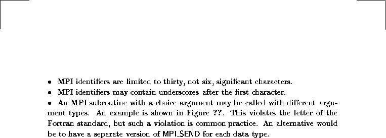
Figure: An example of calling a routine with mismatched formal
and actual arguments.
All MPI named constants can be used
wherever an entity declared with the PARAMETER attribute can be
used in Fortran.
There is one exception to this rule: the MPI constant
MPI_BOTTOM (section
) can only be
MPI_BOTTOM
used as a buffer argument.
Jack Dongarra
Fri Sep 1 06:16:55 EDT 1995
Systems With Weak symbols
Next:
Systems without Weak
Up:
MPI Library Implementation
Previous:
MPI Library Implementation
If the compiler and linker support weak external symbols (e.g. Solaris
2.x, other system V.4 machines), then only a single library is
required through the use of #pragma weak thus
#pragma weak MPI_Send = PMPI_Send
int PMPI_Send(/* appropriate args */)
{
/* Useful content */
}
The effect of this #pragma is to define the external symbol MPI_Send as a weak definition. This means that the linker will
not complain if there is another definition of the symbol (for
instance in the profiling library), however if no other definition
exists, then the linker will use the weak definition.
This type of situation is illustrated in Fig.
, in
which a profiling library has been written that profiles calls to
MPI_Send() but not calls to MPI_Bcast(). On systems with
weak links the link step for an application would be something like
% cc ... -lprof -lmpi
References to MPI_Send() are resolved in the profiling
library, where the routine then calls PMPI_Send() which is
resolved in the MPI library. In this case the weak link to
PMPI_Send() is ignored. However, since MPI_Bcast() is not
included in the profiling library, references to it are
resolved via a weak link to PMPI_Bcast() in the MPI library.

Figure: Resolution of MPI calls on systems with weak links.
Jack Dongarra
Fri Sep 1 06:16:55 EDT 1995
Systems without Weak Symbols
Next:
Complications
Up:
MPI Library Implementation
Previous:
Systems With Weak
In the absence of weak symbols then one possible solution would be to
use the C macro pre-processor thus
#ifdef PROFILELIB
# ifdef __STDC__
# define FUNCTION(name) P##name
# else
# define FUNCTION(name) P/**/name
# endif
#else
# define FUNCTION(name) name
#endif
Each of the user visible functions in the library would then be
declared thus
int FUNCTION(MPI_Send)(/* appropriate args */)
{
/* Useful content */
}
The same source file can then be compiled to produce the MPI and the
PMPI versions of
the library, depending on the state of the PROFILELIB macro
symbol.
It is required that the standard MPI library be built in such a way
that the inclusion of MPI functions can be achieved one at a time.
This is a somewhat unpleasant requirement, since it may mean that
each external function has to be compiled from a separate file.
However this is necessary so that the author of the profiling library
need only define those MPI functions that are to be intercepted,
references to any others being fulfilled by the normal MPI library.
Therefore the link step can look something like this
% cc ... -lprof -lpmpi -lmpi
Here libprof.a contains the profiler functions which intercept
some of the MPI functions. libpmpi.a contains the ``name
shifted'' MPI functions, and libmpi.a contains the normal
definitions of the MPI functions.
Thus, on systems without weak links the example shown in
Fig.
would be resolved as shown in
Fig.

Figure: Resolution of MPI calls on systems without weak links.
Jack Dongarra
Fri Sep 1 06:16:55 EDT 1995
Complications
Next:
Multiple Counting
Up:
Examples
Previous:
Systems without Weak
Jack Dongarra
Fri Sep 1 06:16:55 EDT 1995
Multiple Counting
Next:
Linker Oddities
Up:
Complications
Previous:
Complications
Since parts of the MPI library may themselves be implemented using
more basic MPI functions (e.g. a portable implementation of the
collective operations implemented using point to point communications),
there is potential for profiling functions to be called from within an
MPI function which was called from a profiling function. This could
lead to ``double counting'' of the time spent in the inner routine.
Since this effect could actually be useful under some circumstances
(e.g. it might allow one to answer the question ``How much time is
spent in the point to point routines when they're called from
collective functions ?''), the MPI Forum decided not to enforce any
restrictions on the author of the MPI library which would overcome
this. Therefore, the author of the profiling library should be aware of
this problem, and guard against it. In a single threaded
world this is easily achieved through use of a static variable in the
profiling code which remembers if you are already inside a profiling
routine. It becomes more complex in a multi-threaded environment (as
does the meaning of the times recorded!)
Jack Dongarra
Fri Sep 1 06:16:55 EDT 1995
Linker Oddities
Next:
Multiple Levels of
Up:
Complications
Previous:
Multiple Counting
The Unix linker traditionally operates in one pass. The effect of this
is that functions from libraries are only included in the image if
they are needed at the time the library is scanned. When combined with
weak symbols, or multiple definitions of the same function, this can
cause odd (and unexpected) effects.
Consider, for instance, an implementation of MPI in which the Fortran
binding is achieved by using wrapper functions on top of the C
implementation. The author of the profile library then assumes that it
is reasonable to provide profile functions only for the C binding,
since Fortran will eventually call these, and the cost of the wrappers
is assumed to be small. However, if the wrapper functions are not in
the profiling library, then none of the profiled entry points will be
undefined when the profiling library is called. Therefore none of the
profiling code will be included in the image. When the standard MPI
library is scanned, the Fortran wrappers will be resolved, and will
also pull in the base versions of the MPI functions. The overall
effect is that the code will link successfully, but will not be
profiled.
To overcome this we must ensure that the Fortran wrapper functions are
included in the profiling version of the library. We ensure that this
is possible by requiring that these be separable from the rest of the
base MPI library. This allows them to be extracted out of the base
library and placed into the profiling library using the Unix ar
command.
Jack Dongarra
Fri Sep 1 06:16:55 EDT 1995
Multiple Levels of Interception
Next:
Conclusions
Up:
The MPI Profiling
Previous:
Linker Oddities
The scheme given here does not directly support the nesting of
profiling functions, since it provides only a single alternative name
for each MPI function. The MPI Forum gave consideration to an implementation
which would allow multiple levels of call interception; however, it was
unable to construct an implementation of this which did not
have the following disadvantages

Since one of the objectives of MPI is to permit efficient, low latency
implementations, and it is not the business of a standard to require a
particular implementation language, the MPI Forum decided to accept the scheme
outlined above.
Note, however, that it is possible to use the scheme above to
implement a multi-level system, since the function called by the user
may call many different profiling functions before calling the
underlying MPI function.
Unfortunately such an implementation may require more cooperation
between the different profiling libraries than is required for the
single level implementation detailed above.
Jack Dongarra
Fri Sep 1 06:16:55 EDT 1995
Conclusions
Next:
Design Issues
Up:
MPI: The Complete Reference
Previous:
Multiple Levels of
This book has attempted to give a complete description of the MPI
specification, and includes code examples to illustrate aspects
of the use of MPI. After reading the preceding chapters programmers should
feel comfortable using MPI to develop message-passing applications.
This final chapter addresses some important topics
that either do not easily fit into the other chapters, or which are best
dealt with after a good overall understanding of MPI has been gained.
These topics are concerned more with the interpretation of the MPI
specification, and the rationale behind some aspects of its design, rather
than with semantics and syntax. Future extensions to MPI and the current
status of MPI implementations will also be discussed.
Jack Dongarra
Fri Sep 1 06:16:55 EDT 1995
Design Issues
Next:
Why is MPI
Up:
Conclusions
Previous:
Conclusions
complexity of MPI
Jack Dongarra
Fri Sep 1 06:16:55 EDT 1995
Why is MPI so big?
Next:
Should we be
Up:
Design Issues
Previous:
Design Issues
One aspect of concern,
particularly to novices, is the large number of routines
comprising the MPI
specification. In all there are 128 MPI routines,
and further extensions
(see Section
) will probably
increase their number.
There are two fundamental reasons for the size of MPI.
The first reason is that MPI was designed to be rich in
functionality.
This is reflected in MPI's support for derived datatypes,
modular communication via the communicator abstraction, caching,
application topologies,
and the fully-featured set of collective communication routines.
The second reason for the size of MPI
reflects the diversity and complexity of today's high
performance computers. This is particularly true with respect to the
point-to-point communication
routines where the different communication modes
(see Sections
and
) arise mainly
as a means of providing a set of the most
widely-used communication protocols. For example, the synchronous
communication mode
corresponds closely to a protocol that minimizes the
copying and buffering of
data through a rendezvous mechanism. A protocol
that attempts to initiate delivery of messages as soon as possible
would provide buffering for messages, and this corresponds closely
to the buffered communication mode (or the standard mode if this is
implemented with sufficient buffering).
One could decrease the number of functions by increasing the
number of parameters in each call. But such approach would
increase the call overhead and would make the use of the most
prevalent calls more complex. The availability of a large
number of calls to deal with more esoteric features of MPI
allows one to provide a simpler interface to the more frequently
used functions.
Jack Dongarra
Fri Sep 1 06:16:55 EDT 1995
Should we be concerned about the size of MPI?
Next:
Why does MPI
Up:
Design Issues
Previous:
Why is MPI
There are two potential reasons
why we might be concerned about the size of MPI.
The first is that potential
users might equate size with complexity and decide that MPI is too
complicated to bother learning.
The second is that vendors might decide that
MPI is too difficult to implement.
The design of MPI addresses the first of
these concerns by adopting a layered approach.
For example, novices can
avoid having to worry about groups and
communicators by performing all
communication in the pre-defined communicator MPI_COMM_WORLD.
In fact, most
existing message-passing applications
can be ported to MPI simply by
converting the communication routines
on a one-for-one basis (although the
resulting
MPI application may not be optimally
efficient). To allay the concerns
of potential implementors the MPI Forum at one stage considered
defining a core subset of MPI known as the MPI subset that would
be substantially smaller than MPI and include just the
point-to-point communication routines and a few of the more
commonly-used collective communication routines. However, early work
by Lusk, Gropp, Skjellum, Doss, Franke and others on early
implementations of MPI showed that it
could be fully implemented without a prohibitively
large effort
[16]
[12]. Thus,
the rationale for the MPI subset was lost, and this
idea was dropped.
Jack Dongarra
Fri Sep 1 06:16:55 EDT 1995
Introduction
Next:
The Goals of
Up:
MPI: The Complete Reference
Previous:
Contents
Message passing is a programming paradigm used
widely on parallel computers, especially Scalable Parallel
Computers (SPCs) with
distributed memory, and on Networks of Workstations (NOWs).
Although there are many variations, the basic
concept of processes communicating through messages is well understood.
Over the last ten years, substantial progress has been made in casting
significant applications into this paradigm. Each vendor
has implemented its own variant.
More recently, several public-domain systems have demonstrated
that a message-passing system can be efficiently and
portably implemented.
It is thus an appropriate time to define both the syntax
and semantics of a standard
core of library routines that will be useful to a wide
range of users and efficiently implementable on a wide range of computers.
This effort has been undertaken over the last three years by the
Message Passing Interface (MPI) Forum, a group of more than 80
people from 40 organizations, representing vendors of parallel
systems, industrial users, industrial and national research laboratories,
and universities.
MPI Forum
The designers of MPI sought to make use of the most attractive features
of a number of existing message-passing systems, rather than selecting one of
them and adopting it as the standard.
Thus, MPI has been strongly influenced
by work at the IBM T. J. Watson Research Center
[2]
[1], Intel's NX/2
[24], Express
[23], nCUBE's Vertex
[22], p4
[5]
[6], and
PARMACS
[7]
[3]. Other important contributions have come
from Zipcode
[26]
[25], Chimp
[14]
[13], PVM
[27]
[17], Chameleon
[19],
and PICL
[18]. The MPI Forum
identified some critical shortcomings of existing message-passing
systems, in areas such as complex data layouts or
support for modularity and safe communication.
This led to the introduction of new features in MPI.
The MPI standard defines the user interface and
functionality for a wide range of message-passing capabilities. Since
its completion in June of 1994, MPI has become widely
accepted and used. Implementations are available on a range of
machines from SPCs to NOWs. A growing number of SPCs have an MPI
supplied and supported by the vendor. Because of this, MPI
has achieved one of its goals - adding credibility to parallel
computing. Third party vendors, researchers, and others now have a
reliable and portable way to express message-passing, parallel programs.
The major goal of MPI, as with most standards, is a degree of
portability across different machines.
The expectation is for a degree of portability comparable to that given
by programming languages such as Fortran.
This means that the same message-passing source code
can be executed on a variety of machines as long as the MPI library is
available, while some tuning might be needed to take best advantage of
the features of each system.
portability
Though
message passing is often thought of in the context of
distributed-memory parallel computers, the same code can run well
on a shared-memory parallel computer. It can run on a network of
workstations, or, indeed, as a set of
processes running on a single workstation.
Knowing that efficient MPI
implementations exist across a wide variety of computers gives a
high degree of flexibility in code development, debugging, and
in choosing a platform for production runs.
Another type of compatibility
offered by MPI is the ability to run transparently on heterogeneous
systems, that is, collections of processors with distinct architectures.
It is possible for an MPI implementation to span such
a heterogeneous collection, yet provide a virtual computing model
that hides many architectural differences.
The user need not worry whether the code is sending
messages between processors of like or unlike architecture.
The MPI
implementation will automatically do any necessary data conversion and
utilize the correct communications protocol. However, MPI does
not prohibit implementations that are targeted to a single,
homogeneous system, and does not mandate that distinct
implementations be interoperable.
Users that wish to run on an heterogeneous
system must use an MPI implementation designed to
support heterogeneity.
heterogeneous
interoperability
Portability is central but the standard
will not gain wide usage if this was achieved at the expense of
performance. For example, Fortran is commonly used over assembly
languages because compilers are almost always available that yield
acceptable performance compared to the non-portable alternative of assembly
languages. A crucial point is that MPI was carefully designed
so as to allow efficient implementations. The design
choices seem to have been made correctly,
since MPI implementations over a wide range of
platforms are achieving high performance, comparable to that
of less portable, vendor-specific systems.
An important design goal of MPI was to allow efficient
implementations across machines of differing characteristics.
efficiency
For example, MPI carefully avoids specifying how operations will
take place. It only specifies what an operation does logically. As a
result, MPI can be easily implemented on systems that buffer messages at
the sender, receiver, or do no buffering at all.
Implementations can take advantage of specific features of the
communication subsystem of various machines. On machines with
intelligent communication coprocessors, much of the message passing
protocol can be offloaded to this coprocessor. On other systems,
most of the communication code is executed by the main processor.
Another example is
the use of opaque objects in MPI. By hiding the details of how
MPI-specific objects are represented,
each implementation is free to do whatever is
best under the circumstances.
Another design choice leading to efficiency is the avoidance of
unnecessary work.
MPI was carefully designed so as to avoid a requirement for
large amounts of extra information with each message, or the
need for complex encoding or decoding of message headers.
MPI also avoids extra computation or tests in critical
routines since this can degrade performance. Another way of
minimizing work is to encourage the reuse of previous computations.
MPI provides this capability through constructs such as persistent
communication requests and caching of attributes on communicators.
The design of MPI avoids the need for extra copying and
buffering of data: in many cases, data can be moved from the user
memory directly to the wire, and be received directly from the wire
to the receiver memory.
MPI was designed to encourage overlap of communication and
computation, so as to take advantage of intelligent
communication agents, and to hide communication latencies.
This is achieved by the use of nonblocking
communication calls, which separate the initiation of a
communication from its completion.
Scalability is an important goal of parallel processing.
MPI allows or supports scalability through several of its
design features. For example, an
application can create subgroups of processes that, in turn, allows
collective communication operations to limit their scope to the
processes involved. Another technique used is to
provide functionality without a computation that
scales as the number of processes. For example, a two-dimensional
Cartesian topology can be subdivided into its one-dimensional rows or columns
without explicitly enumerating the processes.
scalability
Finally, MPI, as all good standards, is valuable in that it defines
a known, minimum behavior of message-passing implementations. This
relieves the programmer from having to worry about certain problems
that can arise. One example is
that MPI guarantees that the underlying transmission of messages is
reliable. The user need not check if a message is received
correctly.
Next:
The Goals of
Up:
MPI: The Complete Reference
Previous:
Contents
Jack Dongarra
Fri Sep 1 06:16:55 EDT 1995
C Binding Issues
Next:
Point-to-Point Communication
Up:
Language Binding
Previous:
Fortran 77 Binding
We use the ANSI C declaration format. All MPI names have an MPI_
prefix, defined constants are in all capital letters, and defined types and
functions have one capital letter after the prefix.
Programs must not declare variables or functions with names beginning with
the prefix MPI_ or PMPI_.
This is mandated to avoid possible name collisions.
The definition of named constants, function prototypes, and type
definitions must be supplied in an include file mpi.h.
include filempif.h
Almost all C functions return an error code.
The successful return code will
be MPI_SUCCESS, but
failure return codes are implementation dependent.
A few C functions do not return error codes,
so that they can be implemented as
macros.
return codes
Type declarations are provided for handles to each category of opaque
objects. Either a pointer or an integer type is used.
Array arguments are indexed from zero.
Logical flags are integers with value 0 meaning ``false'' and a non-zero
value meaning ``true.''
Choice arguments are pointers of type void*.
Address arguments are of MPI defined type
MPI_Aint. This is defined to be an int of the size needed to
hold any valid address on the target architecture.
All named MPI constants can be used in initialization expressions or
assignments like C constants.
Jack Dongarra
Fri Sep 1 06:16:55 EDT 1995
Why does MPI not guarantee buffering?
Next:
Portable Programming with
Up:
Design Issues
Previous:
Should we be
buffering
MPI does not guarantee to buffer arbitrary messages because memory is
a finite resource on all computers. Thus, all computers will fail under
sufficiently adverse communication loads. Different computers at different
times are capable of providing differing amounts of buffering, so if
a program relies on buffering it may fail under certain conditions, but
work correctly under other conditions. This is clearly undesirable.
Given that no message passing system can guarantee that messages will
be buffered as required under all circumstances, it might be asked why
MPI does not guarantee a minimum amount of memory available for
buffering. One major problem is that it is not obvious how to
specify the amount of buffer space that is available, nor is it easy
to estimate how much buffer space is consumed by a particular
program.
Different buffering policies make sense in
different environments. Messages can be buffered at the sending
node or at the receiving node, or both. In the former case,
-
buffers can be dedicated to one destination in one
communication domain,
-
or dedicated to one destination
for all communication domains,
-
or shared by all outgoing communications,
-
or shared by all processes running at a processor node,
-
or part of the buffer pool may be dedicated, and part
shared.
Similar choices occur if messages are buffered at
the destination. Communication buffers may be fixed in size, or they
may be allocated dynamically out of the heap, in competition with the
application. The buffer allocation policy may depend on the size
of the messages (preferably buffering short messages), and may depend
on communication history (preferably buffering on busy channels).
The choice of the right policy is strongly dependent on the hardware and
software environment.
For instance, in a dedicated environment, a processor
with a process blocked on a send is idle and so
computing resources are not wasted if this
processor copies the outgoing message to a buffer. In a time shared
environment, the computing resources may be used by another process.
In a system where buffer space can be in paged memory, such space can
be allocated from heap. If the buffer space cannot be paged,
or has to be in kernel space, then a separate buffer
is needed. Flow control may require that
some amount of buffer space be dedicated to each pair of communicating
processes.
The optimal strategy strongly depends on various
performance parameters of the system: the bandwidth, the communication
start-up time, scheduling and context switching overheads, the amount
of potential overlap between communication and computation, etc.
The choice of a buffering and scheduling policy
may not be entirely under the control of the MPI
implementor, as it is partially determined by the properties of the
underlying communication layer.
Also,
experience in this arena is quite limited, and underlying technology
can be expected to change rapidly: fast, user-space
interprocessor communication mechanisms are an active research area
[20]
[28].
Attempts by the MPI Forum to design mechanisms for querying or
setting the amount of buffer space available to standard communication
led to the conclusion that such mechanisms will either restrict
allowed implementations unacceptably, or provide
bounds that will be extremely pessimistic on most implementations in
most cases. Another problem is that parameters such as buffer
sizes work against portability.
Rather then restricting the
implementation strategies for standard communication, the choice was
taken to provide additional communication modes for those users that
do not want to trust the implementation to make the right choice for
them.
Next:
Portable Programming with
Up:
Design Issues
Previous:
Should we be
Jack Dongarra
Fri Sep 1 06:16:55 EDT 1995
Portable Programming with MPI
Next:
Dependency on Buffering
Up:
Conclusions
Previous:
Why does MPI
portable programming
The MPI specification
was designed to make it possible to write portable
message passing
programs while avoiding unacceptable performance degradation.
Within the context of
MPI, ``portable'' is synonymous with ``safe.''
Unsafe programs may exhibit a different behavior on different
systems because they are non-deterministic: Several outcomes
are consistent with the MPI specification, and the actual
outcome to occur depends on the precise timing of events.
Unsafe programs may require resources that are not always
guaranteed by MPI,
in order to complete successfully. On systems where such
resources are unavailable, the program will encounter a
resource error. Such an error will manifest itself as an actual
program error, or will result in deadlock.
There are
three main issues relating to the portability of MPI programs (and, indeed,
message passing programs in general).
-
The program should not depend on the
buffering of messages by MPI or lower
levels of the communication system.
A valid MPI implementation may, or may
not, buffer messages of a given size (in standard mode).
-
The program should not depend upon whether collective communication
routines, such as MPI_Bcast(), act as barrier
synchronizations. In
a valid MPI implementation
collective communication routines may, or may not,
have the side effect of performing a barrier synchronization.
-
The program should
ensure that messages are matched by the intended receive call.
Ambiguities in the
specification of communication can lead to incorrect
or non-deterministic programs since race conditions may arise.
MPI provides message tags
and communicators to help avoid these types of
problem.
If proper attention is not paid to
these factors a message passing code
may fail intermittently on a given computer,
or may work correctly on one
machine but not on another. Clearly such a program is not portable.
We shall now consider each of the above factors in more detail.
Next:
Dependency on Buffering
Up:
Conclusions
Previous:
Why does MPI
Jack Dongarra
Fri Sep 1 06:16:55 EDT 1995
Dependency on Buffering
Next:
Collective Communication and
Up:
Portable Programming with
Previous:
Portable Programming with
buffering
A message passing program is
dependent on the buffering of messages if
its communication graph has a cycle.
The communication graph is a directed graph
in which the nodes represent MPI communication calls
and the edges represent
dependencies between these calls: a directed edge uv indicates
that operation v might not be able to complete before operation u is started.
Calls may be dependent because they have to be executed in
succession by the same process, or because they are matching
send and receive calls.

The execution of the code results in the
dependency graph illustrated in Figure
,
for the case of a three
process group.

Figure: Cycle in communication graph for cyclic shift.
The arrow from each send to the following receive
executed by the same process reflects the program dependency
within each process: the receive call cannot be executed until
the previous send call has completed. The double arrow between
each send and the matching receive reflects their mutual
dependency: Obviously, the receive cannot
complete unless the matching send was invoked. Conversely,
since a standard mode send is used, it may be the case that
the send blocks until a matching receive occurs.
The dependency graph has a cycle.
This code will only work if the system provides sufficient
buffering, in
which case the send operation will complete locally, the call to
MPI_Send() will return,
and the matching call to MPI_Recv()
will be
performed. In the absence of sufficient
buffering MPI does not specify an
outcome, but for most implementations deadlock will occur, i.e., the
call to MPI_Send() will never return: each process will
wait for the next process on the ring to execute a matching
receive.
Thus, the behavior of this code will differ from system to
system, or on the same system, when message size
(count) is changed.
There are a number of ways in which a shift operation can be performed
portably using MPI. These are
-
alternate send and receive calls
(only works if more than one process),
-
use a blocking send in buffered mode,
-
use a nonblocking send and/or receive,
-
use a call to MPI_Sendrecv(),
If at least one process in a shift
operation calls the receive routine before
the send routine, and at least one process calls the send routine
before the receive routine, then at least one communication can proceed,
and, eventually,
the shift will complete successfully.
One of the most efficient ways of doing this is to alternate the send and
receive calls so that all processes
with even rank send first and then
receive, and all processes with odd rank receive first and then send.
Thus, the following code is portable provided there is more than one
process, i.e., clock and anticlock are different:
if (rank%2) {
MPI_Recv (buf2, count, MPI_INT, anticlock, tag, comm, &status);
MPI_Send (buf1, count, MPI_INT, clock, tag, comm);
}
else {
MPI_Send (buf1, count, MPI_INT, clock, tag, comm);
MPI_Recv (buf2, count, MPI_INT, anticlock, tag, comm, &status);
}
The resulting communication graph is illustrated in
Figure
. This graph is acyclic.

Figure: Cycle in communication graph is broken by reordering
send and receive.
If there is only one process then
clearly blocking send and receive routines
cannot be used since the send must be
called before the receive, and so
cannot complete in the absence of buffering.
We now consider methods for
performing shift operations that work even if
there is only one process involved.
A blocking send in buffered mode
can be used to perform a shift operation.
In this case the application program passes a buffer to the MPI
communication system, and
MPI can use this to buffer messages. If the buffer
provided is large enough, then the shift will complete successfully.
The following
code shows how to use
buffered mode to create a portable shift operation.
...
MPI_Pack_size (count, MPI_INT, comm, &buffsize)
buffsize += MPI_BSEND_OVERHEAD
userbuf = malloc (buffsize)
MPI_Buffer_attach (userbuf, buffsize);
MPI_Bsend (buf1, count, MPI_INT, clock, tag, comm);
MPI_Recv (buf2, count, MPI_INT, anticlock, tag, comm, &status);
MPI guarantees that the buffer supplied by a call to
MPI_Buffer_attach()
will be used if it is needed to buffer the message.
(In an implementation
of MPI that provides sufficient buffering,
the user-supplied buffer may be
ignored.)
Each buffered send operations can complete locally, so
that a deadlock will not occur. The acyclic communication graph for
this modified code is shown in Figure
.
Each receive depends on the matching send, but the
send does not depend anymore on the matching receive.

Figure: Cycle in communication graph is broken by using
buffered sends.
Another approach is to use nonblocking communication.
One can either use a
nonblocking send, a nonblocking receive, or both.
If a nonblocking send is
used, the call to MPI_Isend() initiates the send
operation and then returns.
The call to MPI_Recv() can then be made,
and the communication completes
successfully.
After the call to MPI_Isend(), the data in buf1 must
not be changed until one is
certain that the data have been sent or copied
by the system. MPI provides the routines MPI_Wait() and
MPI_Test()
to check on this. Thus, the following code is portable,
...
MPI_Isend (buf1, count, MPI_INT, clock, tag, comm, &request);
MPI_Recv (buf2, count, MPI_INT, anticlock, tag, comm, &status);
MPI_Wait (&request, &status);
The corresponding acyclic communication graph is shown in
Figure
.

Figure: Cycle in communication graph is broken by using
nonblocking sends.
Each receive operation depends on the matching send,
and each wait depends on the matching communication; the send
does not depend on the matching receive, as a nonblocking send
call will return even if no matching receive is posted.
(Posted nonblocking communications do consume resources: MPI
has to keep track of such posted communications. But the
amount of resources consumed is proportional to the number of
posted communications, not to the total size of the pending messages. Good MPI implementations will support a large number of
pending nonblocking communications, so that this will not cause
portability problems.)
An alternative approach is to perform a nonblocking receive first to
initiate (or ``post'') the receive,
and then to perform a blocking send in
standard mode.
...
MPI_Irecv (buf2, count, MPI_INT, anticlock, tag, comm, &request);
MPI_Send (buf1, count, MPI_INT, clock, tag, comm):
MPI_Wait (&request, &status);
The call to MPI_Irecv()
indicates to MPI that incoming data should be
stored in buf2; thus, no buffering is required. The call to
MPI_Wait()
is needed to block until the data has actually been received
into buf2. This alternative code will often result in
improved performance,
since sends complete faster in many implementations
when the matching receive is already posted.
Finally, a portable shift
operation can be implemented using the routine
MPI_Sendrecv(),
which was explicitly designed to send to one process
while receiving from another in a safe and portable way. In this
case only a single call is required;
...
MPI_Sendrecv (buf1, count, MPI_INT, clock, tag,
buf2, count, MPI_INT, anticlock, tag, comm, &status);
Next:
Collective Communication and
Up:
Portable Programming with
Previous:
Portable Programming with
Jack Dongarra
Fri Sep 1 06:16:55 EDT 1995
Collective Communication and Synchronization
Next:
Ambiguous Communications and
Up:
Portable Programming with
Previous:
Dependency on Buffering
collective, semantics of
The MPI specification purposefully does not mandate whether or not
collective communication operations have the side effect of synchronizing
the processes over which they operate. Thus, in one valid implementation
collective communication operations may synchronize processes, while in another
equally valid implementation they do not. Portable MPI programs, therefore,
must not rely on whether or not collective communication operations
synchronize processes. Thus, the following assumptions must be avoided.
-
We assume MPI_Bcast() acts as a barrier synchronization and it doesn't.
MPI_Irecv (buf2, count, MPI_INT, anticlock, tag, comm, &status);
MPI_Bcast (buf3, 1, MPI_CHAR, 0, comm);
MPI_Rsend (buf1, count, MPI_INT, clock, tag, comm);
Here if we want to perform the send in ready mode we must be certain
that the receive has already been initiated at the destination. The above
code is nonportable because if the broadcast does not act as a barrier
synchronization we cannot be sure this is the case.
-
We assume that MPI_Bcast() does not act as a barrier synchronization
and it
does. Examples of this case are given in Examples
,
, and
starting on page
.
Jack Dongarra
Fri Sep 1 06:16:55 EDT 1995
Ambiguous Communications and Portability
Next:
Heterogeneous Computing with
Up:
Portable Programming with
Previous:
Collective Communication and
ambiguity of communications
modularitylibraries, safety
MPI employs the communicator abstraction
to promote software modularity by allowing the
construction of independent communication streams between processes,
thereby ensuring that messages sent in one phase of an application
are not incorrectly intercepted by another phase. Communicators
are particularly important in allowing libraries that make message passing
calls to be used safely within an application.
The point here is that
the application developer has no way of knowing if the tag, group, and rank
completely disambiguate the message traffic of different libraries and
the rest of the application. Communicators, in effect, provide an
additional criterion for message selection, and hence permits the construction
of independent tag spaces.
We discussed in
Section
possible hazards when a library uses
the same communicator as the calling code. The incorrect matching of
sends executed by the caller code with receives executed by the
library occurred because the library code used wildcarded receives.
Conversely, incorrect matches may occur when the caller code uses
wildcarded receives, even if the library code by itself is deterministic.
Consider the
example in Figure
.
If the program behaves correctly
processes 0 and 1 each
receive a message from process 2,
using a wildcarded selection criterion to
indicate that they are prepared to receive a message from any process. The
three processes then pass data around in a ring within the library routine.
If separate communicators are not used for the communication inside and
outside of the library routine
this program may intermittently fail. Suppose we delay the sending
of the second message sent by process 2, for example, by inserting some
computation, as shown in Figure
.
In this case the wildcarded
receive in process 0 is satisfied by a message sent from process 1, rather
than from process 2, and deadlock results.

Figure: Use of communicators. Numbers
in parentheses indicate the process to which data are being sent or received.
The gray shaded area represents the library routine call. In this case
the program behaves as intended. Note that the second message sent by process
2 is received by process 0, and that the message sent by process 0 is
received by process 2.

Figure: Unintended behavior of program. In this case the message from process 2
to process 0 is never received, and deadlock results.
Even if neither caller nor callee use wildcarded receives, incorrect
matches may still occur if a send initiated before the collective
library invocation is to be matched by a receive posted after the
invocation (Ex.
,
page
).
By using a different
communicator in the library routine we can ensure that the program
is executed correctly, regardless of when the processes enter the library
routine.
Next:
Heterogeneous Computing with
Up:
Portable Programming with
Previous:
Collective Communication and
Jack Dongarra
Fri Sep 1 06:16:55 EDT 1995
Heterogeneous Computing with MPI
Next:
MPI Implementations
Up:
Conclusions
Previous:
Ambiguous Communications and
heterogeneous
Heterogeneous computing uses different computers connected by a
network to solve a problem in parallel. With heterogeneous computing
a number of issues arise that are not applicable when using
a homogeneous parallel computer. For example, the computers may
be of differing computational power, so care must be taken to
distribute the work between them to avoid load imbalance. Other
problems may arise because of the different behavior of floating
point arithmetic on different machines. However,
the two most fundamental issues that must be faced in
heterogeneous computing are,
-
incompatible data representation,
-
interoperability of differing implementations of the message passing
layer.
Incompatible data representations arise when computers use different
binary representations for the same number. In MPI all communication
routines have a datatype argument so implementations can use this
information to perform the appropriate representation conversion
when communicating data between computers.
Interoperability refers to the ability of different implementations
of a given piece of software to work together as if they were a single
homogeneous implementation. A
interoperability
prerequisite of interoperability for MPI would be the
standardization of the MPI's internal data structures,
of the communication protocols, of the initialization,
termination and error handling procedures, of the implementation of
collective operations, and so on.
Since this has not been done, there is no support for interoperability
in MPI. In general, hardware-specific implementations of MPI will
not be interoperable. However it is still possible for different
architectures to work together if they both use the same portable MPI
implementation.
Jack Dongarra
Fri Sep 1 06:16:55 EDT 1995
MPI Implementations
Next:
Extensions to MPI
Up:
Conclusions
Previous:
Heterogeneous Computing with
MPI implementationsimplementations
At the time of writing several portable implementations
of MPI exist,
-
the MPICH implementation from Argonne National
Laboratory and Mississippi
State University
[12],
available by anonymous ftp at info.mcs.anl.gov/pub/mpi.
This version is layered on PVM or P4 and can be run on many systems.
-
The CHIMP implementation from Edinburgh Parallel Computing Center,
available by anonymous ftp at
ftp.epcc.ed.ac.uk/pub/chimp/release/chimp.tar.Z.
-
the LAM implementation from the Ohio Supercomputing Center,
a full MPI standard implementation using LAM, a UNIX
cluster computing environment. Available by anonymous ftp
at tbag.osc.edu/pub/lam.
-
The
UNIFY system provides a subset of MPI within the PVM environment,
without sacrificing the PVM calls already available.
Available by anonymous ftp at ftp.erc.msstate.edu/unify.
In addition, hardware-specific MPI implementations exist for the
Cray T3D, the IBM SP-2, The NEC Cinju, and the Fujitsu AP1000.
Information on MPI implementations and other useful
information on MPI can be found on the MPI web pages
at Argonne National Laboratory (http://www.mcs.anl.gov/mpi),
and at Mississippi State Univ (http://www.erc.msstate.edu/mpi). Additional information can be found on the
MPI
newsgroup comp.parallel.mpi and on netlib.
Jack Dongarra
Fri Sep 1 06:16:55 EDT 1995
Extensions to MPI
Next:
References
Up:
Conclusions
Previous:
MPI Implementations
extensionsMPI-2
When the MPI Forum reconvened in March 1995, the main reason was to
produce a new version of MPI that would have significant new
features. The original MPI is being referred to as MPI-1 and the
new effort is being called MPI-2. The need and desire to extend
MPI-1 arose from several factors. One consideration was that the
MPI-1 effort had a constrained scope. This was done to avoid
introducing a standard that was seen as too large and burdensome for
implementors. It was also done to complete
MPI-1 in the Forum-imposed deadline of one year. A second
consideration for limiting MPI-1 was the feeling by many Forum
members that some proposed areas were still under investigation. As a
result, the MPI Forum decided not to propose a standard in these areas for
fear of discouraging useful investigations into improved methods.
The MPI Forum is now actively meeting and discussing extensions to MPI-1
that will become MPI-2. The areas that are currently under
discussion are:
0.1truein
External Interfaces: This will define interfaces to
allow easy extension of MPI with libraries, and facilitate
the implementation of
packages such as debuggers and profilers.
Among the issues considered are mechanisms for defining new
nonblocking operations and mechanisms for accessing internal
MPI information.
One-Sided Communications: This will extend MPI to allow
communication that does not require execution of matching calls
at both communicating processes. Examples of such operations are
put/get operations that allow a process to access data in
another process' memory, messages with interrupts (e.g., active
messages), and Read-Modify-Write operations (e.g., fetch and add).
Dynamic Resource Management:
This will extend MPI to allow the acquisition of computational
resources and the
spawning and destruction of processes after MPI_INIT.
Extended Collective: This will extend the collective calls to be
non-blocking and apply to inter-communicators.
Bindings: This will produce bindings for Fortran 90 and C++.
Real Time: This will provide some support for real time processing.
0.1truein
Since the MPI-2 effort is ongoing, the topics and areas covered are
still subject to change.
The MPI Forum set a timetable at its first meeting in March 1995. The goal
is release of a preliminary version of certain parts of MPI-2 in
December 1995 at Supercomputing '95. This is to include dynamic
processes. The goal of this early
release is to allow testing of the ideas and to receive extended
public comments. The complete version of MPI-2 will be released at
Supercomputing '96 for final public comment. The final version of
MPI-2 is scheduled for release in the spring of 1997.
Next:
References
Up:
Conclusions
Previous:
MPI Implementations
Jack Dongarra
Fri Sep 1 06:16:55 EDT 1995
References
Next:
About this document
Up:
MPI: The Complete Reference
Previous:
Extensions to MPI
References
-
1
-
V. Bala and S. Kipnis.
Process groups: a mechanism for the coordination of and communication
among processes in the Venus collective communication library.
Technical report, IBM T. J. Watson Research Center,
October 1992.
Preprint.
-
2
-
V. Bala, S. Kipnis, L. Rudolph, and Marc Snir.
Designing efficient, scalable, and portable collective communication
libraries.
In SIAM 1993 Conference on Parallel Processing for Scientific
Computing, pages 862-872, March 1993.
-
3
-
Luc Bomans and Rolf Hempel.
The Argonne/GMD macros in FORTRAN for portable parallel
programming and their implementation on the Intel iPSC/2.
Parallel Computing, 15:119-132, 1990.
-
4
-
J. Bruck, R. Cypher, P. Elustond, A. Ho, C-T. Ho, V. Bala, S. Kipnis, , and
M. Snir.
Ccl: A portable and tunable collective communicationlibrary for
scalable parallel computers.
IEEE Trans. on Parallel and Distributed Systems, 6(2):154-164,
1995.
-
5
-
R. Butler and E. Lusk.
User's guide to the p4 programming system.
Technical Report TM-ANL-92/17, Argonne National Laboratory,
1992.
-
6
-
Ralph Butler and Ewing Lusk.
Monitors, messages, and clusters: the p4 parallel programming system.
Journal of Parallel Computing, 20(4):547-564, April 1994.
-
7
-
Robin Calkin, Rolf Hempel, Hans-Christian Hoppe, and Peter Wypior.
Portable programming with the parmacs message-passing library.
Parallel Computing, 20(4):615-632, April 1994.
-
8
-
S. Chittor and R. J. Enbody.
Performance evaluation of mesh-connected wormhole-routed networks
for interprocessor communication in multicomputers.
In Proceedings of the 1990 Supercomputing Conference, pages
647-656, 1990.
-
9
-
S. Chittor and R. J. Enbody.
Predicting the effect of mapping on the communication performance of
large multicomputers.
In Proceedings of the 1991 International Conference on Parallel
Processing, vol. II (Software), pages II-1 - II-4, 1991.
-
10
-
R. Cypher and E. Leu.
The semantics of blocking and nonblocking send and receive
primitives.
In 8th International Parallel Processing Symposium, pages
729-735, April 1994.
-
11
-
J. J. Dongarra, R. Hempel, A. J. G. Hey, and D. W. Walker.
A proposal for a user-level, message passing interface in a
distributed memory environment.
Technical Report TM-12231, Oak Ridge National Laboratory, February
1993.
-
12
-
Nathan Doss, William Gropp, Ewing Lusk, and Anthony Skjellum.
A model implementation of MPI.
Technical report, Argonne National Laboratory, 1993.
-
13
-
Edinburgh Parallel Computing Centre, University of Edinburgh.
CHIMP Concepts, June 1991.
-
14
-
Edinburgh Parallel Computing Centre, University of Edinburgh.
CHIMP Version 1.0 Interface, May 1992.
-
15
-
Message Passing Interface Forum.
MPI: A message-passing interface standard.
International Journal of Supercomputer Applications, 8(3/4),
1994.
Special issue on MPI.
-
16
-
H. Franke, H. Wu, C.E. Riviere, P.Pattnaik, and M. Snir.
MPI programming environment for IBM SP1/SP2.
In 15th International Conference on Distributed Computing
Systems, pages 127-135, June 1995.
-
17
-
A. Geist, A. Beguelin, J. Dongarra, W. Jiang, R. Manchek, and V. Sunderam.
PVM: A Users' Guide and Tutorial for Networked Parallel
Computing.
MIT Press, 1994.
The book is available electronically, the url is ftp://www.netlib.org/pvm3/book/pvm-book.ps.
-
18
-
G. A. Geist, M. T. Heath, B. W. Peyton, and P. H. Worley.
A user's guide to PICL: a portable instrumented communication
library.
Technical Report TM-11616, Oak Ridge National Laboratory,
October 1990.
-
19
-
William D. Gropp and Barry Smith.
Chameleon parallel programming tools users manual.
Technical Report ANL-93/23, Argonne National Laboratory, March 1993.
-
20
-
V. Karamcheti and A.A. Chien.
Software overheads in messaging layers: Where does the time go?
In 6th International Conference on Architectural Support for
Programming Languages and Operating Systems (ASPLOS VI), pages 51-60,
October 1994.
-
21
-
O. Krämer and H. Mühlenbein.
Mapping strategies in message-based multiprocessor systems.
Parallel Computing, 9:213-225, 1989.
-
22
-
nCUBE Corporation.
nCUBE 2 Programmers Guide, r2.0, December 1990.
-
23
-
Parasoft Corporation, Pasadena, CA.
Express User's Guide, version 3.2.5 edition, 1992.
-
24
-
Paul Pierce.
The NX/2 operating system.
In Proceedings of the Third Conference on Hypercube Concurrent
Computers and Applications, pages 384-390. ACM Press, 1988.
-
25
-
A. Skjellum and A. Leung.
Zipcode: a portable multicomputer communication library atop the
reactive kernel.
In D. W. Walker and Q. F. Stout, editors, Proceedings of the
Fifth Distributed Memory Concurrent Computing Conference, pages 767-776.
IEEE Press, 1990.
-
26
-
A. Skjellum, S. Smith, C. Still, A. Leung, and M. Morari.
The Zipcode message passing system.
Technical report, Lawrence Livermore National Laboratory,
September 1992.
-
27
-
V.S. Sunderam, G.A. Geist, J. Dongarra, and R. Manchek.
The PVM concurrent computing system: Evolution, experiences, and
trends.
Parallel Computing, 20(4):531-545, April 1994.
-
28
-
T. von Eicken, D.E. Culler, S.C. Goldstein, and K.E. Shauser.
Active messages: a mechanism for integrated communication and
computation.
In 19th Annual International Symposium on Computer
Architecture, pages 256-266, May 1992.
-
29
-
D. Walker.
Standards for message passing in a distributed memory environment.
Technical Report TM-12147, Oak Ridge National Laboratory,
August 1992.
Jack Dongarra
Fri Sep 1 06:16:55 EDT 1995
<em>About this document ...</em>

Up:
MPI: The Complete Reference
Previous:
References
MPI: The Complete Reference
This document was generated using the
LaTeX2HTML translator Version 0.6.4 (Tues Aug 30 1994) Copyright © 1993, 1994,
Nikos Drakos, Computer Based Learning Unit, University of Leeds.
The command line arguments were:
latex2html book.tex.
The translation was initiated by Jack Dongarra on Fri Sep 1 06:16:55 EDT 1995
Jack Dongarra
Fri Sep 1 06:16:55 EDT 1995
Point-to-Point Communication
Next:
Introduction and Overview
Up:
MPI: The Complete Reference
Previous:
C Binding Issues
Jack Dongarra
Fri Sep 1 06:16:55 EDT 1995
Introduction and Overview
Next:
Blocking Send and
Up:
Point-to-Point Communication
Previous:
Point-to-Point Communication
The basic communication mechanism of MPI is the transmittal of data
between a pair of processes, one side sending, the other, receiving.
We call this ``point to point communication.'' Almost all the
constructs of MPI are built around the point to point operations
and so this chapter is fundamental. It is also quite a long chapter since:
there are many variants to the point to point operations; there
is much to say in terms of the semantics of the operations; and related
topics, such as probing for messages, are explained here because
they are used in conjunction with the point to point operations.
MPI provides a set of send and receive functions that allow
the communication of typedtyped data
data with an associated tag.tagmessage tag
Typing of the message contents is necessary for heterogeneous support -
the type information is needed so that correct data representation
conversions can be performed as data is sent from one architecture to
another. The tag allows selectivity of messages at the receiving end:
one can receive on a particular tag, or one can wild-card this
quantity, allowing reception of messages with any tag. Message
selectivity on the
source process of the message is also provided.
A fragment of C code
appears in Example
for the example of
process 0 sending a message to process 1.
The code executes on both
process 0 and process 1.
Process 0 sends a character string using MPI_Send(). The first three
parameters of the send call
specify the data to be sent: the outgoing data is to
be taken from msg; it consists of strlen(msg)+1 entries,
each of
type MPI_CHAR (The string "Hello there" contains
strlen(msg)=11
significant characters.
In addition, we are also sending the tex2html_html_special_mark_quot''"
string terminator character).
The fourth parameter specifies the message
destination, which is process 1.
The fifth parameter specifies the message tag.
Finally, the last parameter is a
communicatorcommunicator
that specifies a
communication domaincommunication domain
for this communication. Among other
things, a communicator serves to define
a set of processes that can be
contacted.
Each such process is labeled by
a process rank.rank
Process ranks are integers
and are discovered by inquiry to a communicator (see the
call to MPI_Comm_rank()).
MPI_COMM_WORLDMPI_COMM_WORLD
is a default communicator provided
upon start-up that defines an initial
communication domain for all the processes
that participate in the computation.
Much more will be said about
communicators in Chapter
.
The receiving process specified
that the incoming data was to be placed in msg and that it had a maximum
size of 20 entries, of type MPI_CHAR.
The variable status, set by MPI_Recv(), gives information
on the source and tag of the message and how many elements were
actually received.
For example, the receiver can examine this variable to find out the
actual length of the character string received.
Datatype matchingdatatype matchingtype matching
(between sender and receiver) and data
conversion data conversionrepresentation conversion
on heterogeneous systems
are discussed in more detail in Section
.

The Fortran version of this code is shown in
Example
. In order to make our
Fortran examples more readable, we use Fortran 90
syntax, here and in
many other places in this book. The examples can be
easily rewritten in standard Fortran 77. The Fortran code is
essentially identical to the C code. All MPI calls are
procedures, and an additional parameter is used to return
the value returned by the corresponding C
function. Note that Fortran
strings have fixed size and are not
null-terminated.
The receive operation stores "Hello there" in the first
11 positions of msg.

These examples employed blocking blocking
send and receive functions. The send call
blocks until the send buffer can be reclaimed (i.e., after the send, process 0
can safely over-write the contents of msg). Similarly, the
receive function blocks until the receive buffer actually contains the contents
of the message. MPI also provides nonblockingnonblocking send and receive
functions that allow the possible overlap of message transmittal with
computation, or the overlap of multiple message transmittals with one-another.
Non-blocking functions always come in two parts: the posting functions,
posting
which begin the requested operation; and the test-for-completion
functions,test-for-completion which allow the application program to discover whether
the requested operation has completed.
Our chapter begins by explaining blocking functions in detail, in
Section
-
,
while nonblocking functions are covered
later, in Sections
-
.
We have already said rather a lot about a simple transmittal of data
from one process to another, but there is even more. To
understand why, we examine two aspects of the communication: the semantics
semantics
of the communication primitives, and the underlying protocols that
protocols
implement them. Consider the previous example, on process 0, after
the blocking send has completed. The question arises: if the send has
completed, does this tell us anything about the receiving process? Can we
know that the receive has finished, or even, that it has begun?
Such questions of semantics are related to the nature of the underlying
protocol implementing the operations. If one wishes to implement
a protocol minimizing the copying and buffering of data, the most natural
semantics might be the ``rendezvous''rendezvous
version, where completion of the send
implies the receive has been initiated (at least). On the other
hand, a protocol that
attempts to block processes for the minimal amount of time will
necessarily end up doing more buffering and copying of data and will
have ``buffering'' semantics.buffering
The trouble is, one choice of
semantics is not best for all applications, nor is it best for all
architectures. Because the primary goal of MPI is to standardize the
operations, yet not sacrifice performance, the decision was made to
include all the major choices for point to point semantics in the
standard.
The above complexities are manifested in MPI by the existence of
modesmodes for point to point communication. Both blocking and
nonblocking communications have modes. The mode allows one to choose the
semantics of the send operation and, in effect, to influence the
underlying protocol of the transfer of data.
In standard modestandard mode the completion of the send does not
necessarily mean that the matching receive has started, and no
assumption should be made in the application program about whether the
out-going data is buffered by MPI. In buffered mode
buffered mode the user can
guarantee that a certain amount of buffering space is available. The
catch is that the space must be explicitly provided by the application
program. In synchronous mode synchronous mode
a rendezvous semantics between
sender and receiver is used. Finally, there is ready mode.
ready mode This
allows the user to exploit extra knowledge to simplify the protocol and
potentially achieve higher performance. In a ready-mode send, the user
asserts that the matching receive already has been posted.
Modes are covered in Section
.
Next:
Blocking Send and
Up:
Point-to-Point Communication
Previous:
Point-to-Point Communication
Jack Dongarra
Fri Sep 1 06:16:55 EDT 1995
Blocking Send and Receive Operations
Next:
Blocking Send
Up:
Point-to-Point Communication
Previous:
Introduction and Overview
This section describes standard-mode, blocking sends and receives.
Jack Dongarra
Fri Sep 1 06:16:55 EDT 1995
Blocking Send
Next:
Send Buffer and
Up:
Blocking Send and
Previous:
Blocking Send and
send

MPI_Send(void* buf, int count, MPI_Datatype datatype, int dest, int tag, MPI_Comm comm)
MPI_SEND(BUF, COUNT, DATATYPE, DEST, TAG, COMM, IERROR)<type> BUF(*)
INTEGER COUNT, DATATYPE, DEST, TAG, COMM, IERROR
MPI_SEND performs a standard-mode, blocking send.
The semantics of this function are described in
Section
.
The arguments to MPI_SEND are described in
the following subsections.
Jack Dongarra
Fri Sep 1 06:16:55 EDT 1995
Send Buffer and Message Data
Next:
Message Envelope
Up:
Blocking Send and
Previous:
Blocking Send
The send buffersend bufferbuffer, send
specified by MPI_SEND consists of
count successive entries of the type indicated by
datatype,datatype starting
with the entry at address buf. Note that we specify the
message length
in terms of number of entries, not number of bytes. The former is
machine independent and facilitates portable programming.
The count may be zero,
in which case the data part of the message is empty.
The basic datatypes correspond to
the basic datatypes of the host language.
Possible values of this argument for Fortran and the
corresponding Fortran types are listed below.

MPI_INTEGER
MPI_REAL
MPI_DOUBLE_PRECISION
MPI_COMPLEX
MPI_LOGICAL
MPI_CHARACTER
MPI_BYTE
MPI_PACKED
Possible values for this argument for C and the corresponding C
types are listed below.

MPI_CHAR
MPI_SHORT
MPI_INT
MPI_LONG
MPI_UNSIGNED_CHAR
MPI_UNSIGNED_SHORT
MPI_UNSIGNED
MPI_UNSIGNED_LONG
MPI_FLOAT
MPI_DOUBLE
MPI_LONG_DOUBLE
MPI_BYTE
MPI_PACKED
The datatypes MPI_BYTE and MPI_PACKED do not correspond to a
Fortran or C datatype. A value of type MPI_BYTE consists of a byte
(8 binary digits). A
byte is uninterpreted and is different from a character.
Different machines may have
different representations for characters, or may use more than one
byte to represent characters. On the other hand, a byte has the same
binary value on all machines.
The use of MPI_PACKED is explained in
MPI_PACKED
Section
.
MPI requires support of the datatypes listed above, which match the basic
datatypes of Fortran 77 and ANSI C.
Additional MPI datatypes should be provided if the host language has
additional data types. Some examples are:
MPI_LONG_LONG, for C integers declared to be of type
MPI_LONG_LONG
longlong;
MPI_DOUBLE_COMPLEX for double precision complex in
MPI_DOUBLE_COMPLEX
Fortran declared to be of type DOUBLE COMPLEX;
MPI_REAL2,
MPI_REAL2
MPI_REAL4 and MPI_REAL8 for Fortran reals, declared to be of
MPI_REAL4
MPI_REAL8
type REAL*2, REAL*4 and REAL*8, respectively;
MPI_INTEGER1 MPI_INTEGER2 and
MPI_INTEGER4 for Fortran integers, declared to be of type
MPI_INTEGER1
MPI_INTEGER2
MPI_INTEGER4
INTEGER*1, INTEGER*2 and INTEGER*4, respectively.
In addition, MPI provides a mechanism for users to define new, derived,
datatypes. This is explained in Chapter
.
Next:
Message Envelope
Up:
Blocking Send and
Previous:
Blocking Send
Jack Dongarra
Fri Sep 1 06:16:55 EDT 1995
Message Envelope
Next:
Comments on Send
Up:
Blocking Send and
Previous:
Send Buffer and
In addition to data, messages carry information that is used to
distinguish and selectively receive them. This information consists
of a fixed number of fields, which we collectively call
the message envelope. These fields are
message envelope
source, destination, tag, and communicator.
sourcedestinationtagcommunicator
The message source is implicitly determined by the identity of the
message source
message sender. The other fields are specified by arguments in the send
operation.
The comm argument specifies the communicator used for
communicator
the send operation. The communicator is a local object that
represents a communication domain. A communication domain is a
communication domain
global, distributed structure that allows processes in a group
groupprocess group
to communicate with each other, or to communicate with processes in another
group. A communication domain of the first type (communication within a
group) is represented by
an intracommunicator, whereas a communication domain of the second type
intracommunicator
(communication between groups) is represented by an intercommunicator.
intercommunicator
Processes
in a group are ordered, and are identified by their integer rank.
rankprocess rank
Processes may participate in several communication domains; distinct
communication
domains may have partially or even completely overlapping groups of processes.
Each communication domain supports a disjoint stream of communications.
Thus, a process may be able to communicate with another process via two distinct
communication domains, using two distinct communicators. The same
process may be identified by a different rank in the two domains;
and communications in the two domains do not interfere.
MPI applications begin with a default communication domain that includes
all processes (of this parallel job); the default communicator
MPI_COMM_WORLD represents this communication domain.
MPI_COMM_WORLD
Communicators are explained further in Chapter
.
The message destination is specified by the dest
destinationmessage destination
argument.
The range of valid values for dest is
0,...,n-1, where n is the number of
processes in the group.
This range includes the rank of the
sender: if comm is an intracommunicator, then a process may send a
message to itself. If the communicator is an intercommunicator,
then destinations are identified by their rank in the remote group.
The integer-valued message tag is specified by the tag argument.
tagmessage tag
This integer can be used by the application to distinguish messages.
The range of valid tag values is 0,...,UB, where the value of UB is
implementation dependent. It is found by querying the
value of the attribute MPI_TAG_UB, as
MPI_TAG_UB
described in Chapter
.
MPI requires that UB be no less than 32767.
Next:
Comments on Send
Up:
Blocking Send and
Previous:
Send Buffer and
Jack Dongarra
Fri Sep 1 06:16:55 EDT 1995
Comments on Send
Next:
Blocking Receive
Up:
Blocking Send and
Previous:
Message Envelope
Jack Dongarra
Fri Sep 1 06:16:55 EDT 1995
Blocking Receive
Next:
Receive Buffer
Up:
Blocking Send and
Previous:
Comments on Send
receive

MPI_Recv(void* buf, int count, MPI_Datatype datatype, int source, int tag, MPI_Comm comm, MPI_Status *status)
MPI_RECV(BUF, COUNT, DATATYPE, SOURCE, TAG, COMM, STATUS, IERROR)<type> BUF(*)
INTEGER COUNT, DATATYPE, SOURCE, TAG, COMM, STATUS(MPI_STATUS_SIZE), IERROR
MPI_RECV performs a standard-mode, blocking receive.
The semantics of this function are described in
Section
.
The arguments to MPI_RECV are described in
the following subsections.
Jack Dongarra
Fri Sep 1 06:16:55 EDT 1995
Receive Buffer
Next:
Message Selection
Up:
Blocking Send and
Previous:
Blocking Receive
The receive buffer consists of
receive bufferbuffer, receive
storage sufficient to contain count consecutive entries of the type
specified by datatype, starting at address buf.
The length of the received message must be less than or equal to the length of
the receive buffer. An overflow error occurs if all incoming data does
overflow
not fit, without truncation, into the receive buffer.
We explain in Chapter
how to check for errors.
If a
message that is shorter than the receive buffer arrives, then the incoming
message is stored in the initial locations of the receive buffer,
and the remaining locations are not modified.
Jack Dongarra
Fri Sep 1 06:16:55 EDT 1995
The Goals of MPI
Next:
Who Should Use
Up:
Introduction
Previous:
Introduction
The goal of the Message Passing Interface, simply stated, is to
develop a widely used
standard for writing message-passing programs.
As such the interface should
establish a practical, portable, efficient, and flexible standard for message
passing.
A list of the goals of MPI appears below.
Jack Dongarra
Fri Sep 1 06:16:55 EDT 1995
Message Selection
Next:
Return Status
Up:
Blocking Send and
Previous:
Receive Buffer
The selection of a message by a receive operation is governed by
selectionmessage selection
the value of its message envelope.
A message can be received
if its envelope matches the source, tag and
comm values specified by the
receive operation. The receiver may specify a wildcard
wildcard
value for source (MPI_ANY_SOURCE),
MPI_ANY_SOURCE
and/or
a wildcard value for tag (MPI_ANY_TAG),
MPI_ANY_TAG
indicating that any source and/or tag are acceptable. One cannot specify a
wildcard value for comm.
The argument source, if different from MPI_ANY_SOURCE,
sourcemessage source
is specified as a rank within the process group associated
with the communicator (remote process group, for intercommunicators).
The range of valid values for the
source argument is
{0,...,n-1} {MPI_ANY_SOURCE}, where
n is the number of processes in this group.
This range includes the receiver's rank: if comm is an
intracommunicator, then a process may receive a
message from itself. The range of valid values for the tag argument is
{0,...,UB}
{MPI_ANY_TAG}.
tagmessage tag
{MPI_ANY_SOURCE}, where
n is the number of processes in this group.
This range includes the receiver's rank: if comm is an
intracommunicator, then a process may receive a
message from itself. The range of valid values for the tag argument is
{0,...,UB}
{MPI_ANY_TAG}.
tagmessage tag
Jack Dongarra
Fri Sep 1 06:16:55 EDT 1995
Return Status
Next:
Comments on Receive
Up:
Blocking Send and
Previous:
Message Selection
statusreturn status
The receive call does not specify the size of an
incoming message, but only an upper bound. The
source or tag of a received message may not be known if
wildcard values were used in a receive operation.
Also, if multiple requests
are completed by a single MPI function (see
Section
), a distinct error code may be
error code
returned for each request. (Usually, the error code is returned as
the value of the function in C, and as the value of the
IERROR argument in Fortran.)
This information is returned by the status argument of
MPI_RECV.
The type of status is defined by MPI.
Status variables need to be explicitly
allocated by the user, that is, they are not system objects.
In C, status is a structure of type MPI_Status
that contains three fields named
MPI_SOURCE, MPI_TAG, and MPI_ERROR;
the structure may contain
additional fields. Thus, status.MPI_SOURCE,
status.MPI_TAG and status.MPI_ERROR
contain the source, tag and error code, respectively, of
the received message.
In Fortran, status is an array of INTEGERs of length
MPI_STATUS_SIZE. The three constants MPI_SOURCE,
MPI_STATUS_SIZE
MPI_TAG and MPI_ERROR
MPI_SOURCE
MPI_TAG
MPI_ERROR
are the indices of the entries that store the
source, tag and error fields. Thus status(MPI_SOURCE),
status(MPI_TAG) and status(MPI_ERROR)
contain,
respectively, the source, the
tag and the error code of the received message.
The status argument also returns information on the length of the message
received. However, this information is not directly available as a field
of the status variable and a call to MPI_GET_COUNT is required
to ``decode'' this information.

MPI_Get_count(MPI_Status *status, MPI_Datatype datatype, int *count)
MPI_GET_COUNT(STATUS, DATATYPE, COUNT, IERROR)INTEGER STATUS(MPI_STATUS_SIZE), DATATYPE, COUNT, IERROR
MPI_GET_COUNT takes as input the status set
by MPI_RECV and computes
the number of entries received. The number of entries
is returned in count.
The datatype argument should match the argument
provided to the receive call that set status.
(Section
explains that
MPI_GET_COUNT may return, in certain situations, the value
MPI_UNDEFINED.)
MPI_UNDEFINED
Next:
Comments on Receive
Up:
Blocking Send and
Previous:
Message Selection
Jack Dongarra
Fri Sep 1 06:16:55 EDT 1995
Comments on Receive
Next:
Datatype Matching and
Up:
Blocking Send and
Previous:
Return Status
Note the asymmetry between send and receive operations. A receive
asymmetry
operation may
accept messages from an arbitrary sender, but
a send operation
must specify a unique receiver. This matches a ``push'' communication
mechanism, where data transfer is effected by the sender, rather than a
``pull'' mechanism, where data transfer is effected by the receiver.
Source equal to destination is allowed, that is, a process can send a
message to itself.
However, for such a communication to succeed, it is required that the message be
buffered by the system between the completion of the send call and the
start of the receive call. The amount of buffer space available and the buffer
allocation policy are implementation dependent.
Therefore, it is unsafe
and non-portable to send
self-messages with the standard-mode, blocking send and receive
self messagemessage, self
operations described so far, since this may lead to deadlock.
More discussions of this appear in Section
.

Jack Dongarra
Fri Sep 1 06:16:55 EDT 1995
Datatype Matching and Data Conversion
Next:
Type Matching Rules
Up:
Point-to-Point Communication
Previous:
Comments on Receive
type matchingmatching, type
conversion
Jack Dongarra
Fri Sep 1 06:16:55 EDT 1995
Type Matching Rules
Next:
Type MPI_CHARACTER
Up:
Datatype Matching and
Previous:
Datatype Matching and
One can think of message transfer as consisting of the following three phases.

Type matching must be observed at each of these phases. The type
of each variable in the sender buffer must match
the type specified for that entry by the send operation.
The type specified by the send operation must match the type specified by
the receive operation. Finally,
the type of each
variable in the receive buffer must match the type specified for
that entry by the receive operation.
A program that fails to observe these
rules is erroneous.
To define type matching precisely, we need to deal with two issues:
matching of types of variables of the host language with types specified in
communication operations,
and matching of types between sender and receiver.
The types between a send and receive match if
both operations specify identical type names. That is, MPI_INTEGER
matches MPI_INTEGER, MPI_REAL matches MPI_REAL,
and so on. The one exception to this rule is that
the type MPI_PACKED can match
any other type (Section
).
The type of a variable matches the type specified in the
communication operation
if the datatype name used by that operation corresponds
to the basic type of the host program variable. For example, an entry with type
name MPI_INTEGER matches a Fortran variable of type INTEGER.
Tables showing this correspondence for Fortran and C appear in
Section
.
There are two exceptions to this rule: an entry with type name
MPI_BYTE or MPI_PACKED can be used to match
any byte of storage (on a byte-addressable machine),
MPI_PACKEDMPI_BYTE
irrespective of the datatype of the variable that contains this byte.
The type MPI_BYTE allows one to transfer the binary value of a byte in
memory unchanged.
The type MPI_PACKED is used to send data that has been
explicitly packed with calls to MPI_PACK, or receive data that will
be explicitly unpacked with calls to
MPI_UNPACK (Section
).
The following examples illustrate type matching.


Next:
Type MPI_CHARACTER
Up:
Datatype Matching and
Previous:
Datatype Matching and
Jack Dongarra
Fri Sep 1 06:16:55 EDT 1995
Type MPI_CHARACTER
Next:
Data Conversion
Up:
Type Matching Rules
Previous:
Type Matching Rules
MPI_CHARACTER
The
type MPI_CHARACTER matches one character of a Fortran variable of
MPI_CHARACTER
type CHARACTER, rather then the entire character string stored in the
variable. Fortran variables of type CHARACTER
or substrings are transferred as if they were arrays of characters.
This is illustrated in the example below.


Jack Dongarra
Fri Sep 1 06:16:55 EDT 1995
Data Conversion
Next:
Comments on Data
Up:
Datatype Matching and
Previous:
Type MPI_CHARACTER
data conversion
One of the goals of MPI is to support parallel computations across
heterogeneous environments. Communication in a heterogeneous
heterogeneous
environment may require data conversions.
We use the following terminology.
- Type conversion
- changes the datatype of a value, for example,
by rounding a REAL to an INTEGER.
type conversionconversion, type
- Representation conversion
- changes the binary representation of a value,
for example, changing byte ordering, or changing 32-bit floating point
to 64-bit floating point.
representation conversionconversion, representation
The type matching rules imply that MPI communications never do type
conversion. On the other hand, MPI requires that a representation
conversion be
performed when a typed value is transferred across environments that use
different representations for such a value.
MPI does not specify the detailed rules for representation
conversion. Such a conversion is
expected to preserve integer, logical or character values, and to
convert a floating point value to the nearest value that can be
represented on the target system.
Overflow and underflow exceptions may occur during floating point conversions.
overflowunderflow
Conversion of integers or characters may also lead to exceptions when a value
that can be represented in one system cannot be represented in the other
system. An exception
occurring during representation conversion results in a failure of the
communication. An error occurs either in the send operation, or the receive
operation, or both.
If a value sent in a message is untyped (i.e., of type MPI_BYTE),
MPI_BYTE
MPI_BYTE
then the binary representation of the byte stored at the receiver is
identical to the binary representation of the byte loaded at the sender. This
holds true, whether sender and receiver run in the same or in distinct
environments. No representation conversion is done.
Note that representation conversion may
occur when values of type MPI_CHARACTER or
MPI_CHAR are transferred, for example, from an
EBCDIC encoding to an ASCII encoding.
MPI_CHARACTER
MPI_CHAR
No representation conversion need occur when an MPI program executes in
a homogeneous system, where all processes run in the same environment.
Consider the three examples,
-
.
The first program is correct, assuming that a and b are
REAL arrays of size  .
If the sender and receiver execute in different environments,
then the ten real values that are fetched from the send buffer will
be converted to the representation for reals on the receiver site
before they are stored in the receive buffer. While the
number of real elements fetched from the send buffer equal the
number of real elements stored in the receive buffer, the number of
bytes stored need not equal the number of bytes loaded. For example, the
sender may use a four byte representation and the receiver an eight
byte representation for reals.
.
If the sender and receiver execute in different environments,
then the ten real values that are fetched from the send buffer will
be converted to the representation for reals on the receiver site
before they are stored in the receive buffer. While the
number of real elements fetched from the send buffer equal the
number of real elements stored in the receive buffer, the number of
bytes stored need not equal the number of bytes loaded. For example, the
sender may use a four byte representation and the receiver an eight
byte representation for reals.
The second program is erroneous, and its behavior is undefined.
The third program is correct. The exact same
sequence of forty bytes that were loaded from the send buffer will be
stored in the receive buffer, even
if sender and receiver run in a different environment. The message
sent has exactly the same length (in bytes) and the same binary
representation as the message received. If a and b are
of different types,
or if they are of the same type but different data representations are used,
then the bits stored in the receive buffer may encode values that are
different from the values they encoded in the send buffer.
Representation conversion also applies to the envelope of a message.
The source, destination and tag are all integers that may need to be converted.
MPI does not require support for inter-language
communication. The behavior of a program is undefined if messages are sent
by a C process and received by a Fortran process, or vice-versa.
inter-language communication
Next:
Comments on Data
Up:
Datatype Matching and
Previous:
Type MPI_CHARACTER
Jack Dongarra
Fri Sep 1 06:16:55 EDT 1995
Comments on Data Conversion
Next:
Semantics of Blocking
Up:
Datatype Matching and
Previous:
Data Conversion

Jack Dongarra
Fri Sep 1 06:16:55 EDT 1995
Semantics of Blocking Point-to-point
Next:
Buffering and Safety
Up:
Point-to-Point Communication
Previous:
Comments on Data
semantics
This section describes the main properties of the send and receive calls
introduced in Section
.
Interested readers can find a more formal treatment of the issues
in this section in
[10].
Jack Dongarra
Fri Sep 1 06:16:55 EDT 1995
Buffering and Safety
Next:
Multithreading
Up:
Semantics of Blocking
Previous:
Semantics of Blocking
bufferingsafety
The receive described in Section
can be started
whether or not a matching send has been posted.
That version of receive is blocking.
blocking
It returns only after the receive buffer contains the newly received
message. A receive could complete before the matching send
has completed (of course, it can complete only after the matching send
has started).
The send operation described in Section
can be started whether or not a
matching receive has been posted. That version of send
is blocking.
It does not return until the message data
and envelope have been safely stored away so that the sender is
free to access and overwrite the send buffer.
The send call is also potentially non-local.
non-local
The message might be copied directly into the matching receive buffer,
or it might be copied into a temporary system buffer. In the first case, the
send call will not complete until a matching receive call occurs, and so,
if the
sending process is single-threaded, then it will be blocked until this time.
In the
second case, the send call may return ahead of the matching receive call,
allowing a single-threaded process to continue with its computation.
The MPI implementation may make either of these
choices. It might
block the sender or it might buffer the data.
Message buffering
decouples the send and receive operations. A blocking send might
complete as soon
as the message was buffered, even if no matching receive has been executed
by the receiver. On the other hand, message buffering can be expensive,
as it entails additional memory-to-memory copying, and it requires the
allocation of memory for buffering. The choice of the right amount of buffer
space to allocate for communication and of the buffering policy to use is
application and implementation dependent. Therefore, MPI
offers the choice of
several communication modes that allow one to control the choice of the
communication protocol. Modes are described in
communication modesmodescommunication protocol
protocol, communication
Section
. The choice of a buffering policy for the
standard mode send described in
standard modemode, standard
Section
is left to the implementation.
In any case, lack of buffer space will not cause a standard send
call to fail, but will merely cause it to block. In well-constructed
programs, this results in a useful throttle effect.
throttle effect
Consider a situation where a producer repeatedly produces
new values and sends them to a consumer. Assume that the producer produces
new values faster than the consumer can consume them.
If standard sends are used, then the producer will be automatically throttled,
as its send operations will block when buffer space is unavailable.
In ill-constructed programs, blocking may
lead to a deadlock situation, where all processes are
deadlock
blocked, and no progress occurs. Such programs may complete
when sufficient buffer space is available, but will fail on systems
that do less buffering, or when data sets (and message sizes) are increased.
Since any
system will run out of buffer resources as message sizes are increased,
and some implementations may want to provide little buffering, MPI
takes the position that safe programs
safe program
do not rely on system buffering, and will complete correctly irrespective of
the buffer allocation policy used by MPI. Buffering may change the
buffering
performance of a safe program, but it doesn't affect the
result of the program.
MPI does not enforce a safe programming style.
Users are free to take advantage of knowledge of the buffering policy of an
implementation in order to relax the safety requirements, though
doing so will lessen the portability of the program.
The following examples illustrate safe programming issues.


Next:
Multithreading
Up:
Semantics of Blocking
Previous:
Semantics of Blocking
Jack Dongarra
Fri Sep 1 06:16:55 EDT 1995
Who Should Use This Standard?
Next:
What Platforms are
Up:
Introduction
Previous:
The Goals of
The MPI standard is intended for use by all those who want to write portable
message-passing programs in Fortran 77 and C.
This includes individual application programmers,
developers of software designed to run on
parallel machines, and creators of
environments and tools. In order to be
attractive to this wide audience, the standard must provide a simple, easy-to-use
interface for the basic user while not semantically precluding the
high-performance message-passing operations available on advanced machines.
Jack Dongarra
Fri Sep 1 06:16:55 EDT 1995
Multithreading
Next:
Order
Up:
Semantics of Blocking
Previous:
Buffering and Safety
threads
MPI does not specify the interaction of blocking communication calls with the
thread scheduler in a multi-threaded implementation of MPI. The desired
behavior is that a blocking communication call blocks only the issuing thread,
allowing another thread to be scheduled. The blocked thread will be
rescheduled
when the blocked call is satisfied. That is,
when data has been copied out of the
send buffer, for a send operation, or copied into the receive buffer, for a
receive operation. When a thread executes concurrently with a blocked
communication operation,
it is the user's responsibility not to access or modify a
communication buffer until the communication completes.
Otherwise, the outcome of the computation is undefined.
Jack Dongarra
Fri Sep 1 06:16:55 EDT 1995
Order
Next:
Progress
Up:
Semantics of Blocking
Previous:
Multithreading
ordermessage order
Messages are non-overtaking.
Conceptually, one may think of successive
messages sent by a process to another process as ordered in a sequence.
Receive operations posted by a process are also ordered in a sequence. Each
incoming message matches the first matching receive in the sequence. This is
illustrated in Figure
.
Process zero sends two messages to process one and process two sends three
messages to process one.
Process one posts five receives. All communications occur in
the same communication domain. The first message sent by process zero
and the first message sent by process two can be received in either
order, since the first two posted receives match either. The second
message of process two will be received before the third message, even
though the third and fourth receives match either.

Figure: Messages are matched in order.
Thus, if a sender sends two messages in succession to the same destination,
and both match the same receive, then the receive cannot get the
second message if the first message is still pending.
If a receiver posts two receives in succession, and both match the same
message,
then the second receive operation cannot be satisfied by this message, if the
first receive is still pending.
These requirements further define message matching.
matchingmessage matching
They guarantee that message-passing code is deterministic, if processes are
single-threaded and the wildcard MPI_ANY_SOURCE is
MPI_ANY_SOURCE
not used in receives.
Some other MPI functions, such as MPI_CANCEL or
MPI_WAITANY, are additional sources of nondeterminism.
deterministic programs
In a single-threaded process all communication operations are ordered
according to program execution order.
The situation is different when processes are multi-threaded.
order, with threads
The semantics of thread execution may not define
a relative order between two communication operations executed by two
distinct threads. The operations are logically concurrent, even if one
physically precedes the other. In this case, no order constraints
apply. Two messages sent by concurrent threads can be
received in any order. Similarly, if two receive operations that are logically
concurrent receive two successively sent messages, then the two messages can
match the receives in either order.
It is important to understand what is guaranteed by the ordering
property and what is not. Between any pair of communicating
processes, messages flow in order. This does not imply a consistent, total
order on communication events in the system. Consider the following example.


Figure: Order preserving is not transitive.
Next:
Progress
Up:
Semantics of Blocking
Previous:
Multithreading
Jack Dongarra
Fri Sep 1 06:16:55 EDT 1995
Progress
Next:
Fairness
Up:
Semantics of Blocking
Previous:
Order
progress
If a pair of
matching send and receives have been initiated on two processes, then at
least one of these two operations will complete, independently of
other actions in the system. The send operation will
complete, unless the receive is satisfied by another message.
The receive operation will complete, unless the message sent
is consumed by another
matching receive posted at the same destination process.

Jack Dongarra
Fri Sep 1 06:16:55 EDT 1995
Fairness
Next:
Example - Jacobi
Up:
Semantics of Blocking
Previous:
Progress
fairnessstarvation
MPI makes no guarantee of fairness in the handling of
communication. Suppose that a send is posted. Then it is possible
that the destination process repeatedly posts a receive that matches this
send, yet the message is never received, because it is repeatedly overtaken by
other messages, sent from other sources. The scenario requires that the
receive used the wildcard MPI_ANY_SOURCE as its source argument.
MPI_ANY_SOURCE
Similarly, suppose that a
receive is posted by a multi-threaded process. Then it is possible that
messages that
match this receive are repeatedly consumed, yet the receive is never satisfied,
because it is overtaken by other receives posted at this node by
other threads. It is the programmer's responsibility to prevent
starvation in such situations.
Jack Dongarra
Fri Sep 1 06:16:55 EDT 1995
Example - Jacobi iteration
Next:
Send-Receive
Up:
Point-to-Point Communication
Previous:
Fairness
Jacobi
We shall use the following example to illustrate the material
introduced so far, and to motivate new functions.

Since this code has a simple structure, a data-parallel approach can be
used to derive an equivalent parallel code. The array is distributed
across processes, and each process is assigned the task of updating
the entries on the part of the array it owns.
A parallel
algorithm is derived from a choice of data distribution. The
data distribution
distribution should be balanced, allocating (roughly) the same number
of entries to each processor; and it should minimize communication.
Figure
illustrates two possible distributions: a
1D (block) distribution, where the matrix is partitioned in one dimension,
and a 2D (block,block) distribution, where the matrix is partitioned
in two dimensions.

Figure: Block partitioning of a matrix.
Since the communication occurs at block
boundaries, communication volume is minimized by the 2D partition which
has a better area to perimeter ratio. However, in this partition, each
processor communicates with four neighbors, rather than two neighbors
in the 1D partition. When the ratio of n/P (P number of
processors) is small, communication time will be dominated by the
fixed overhead per message, and the first partition will lead to
better performance. When the ratio is large, the second partition
will result in better performance. In order to keep the example
simple, we shall use the first partition; a realistic code would use a
``polyalgorithm'' that selects one of the two partitions, according to
problem size, number of processors, and communication performance
parameters.
The value of each point in the array B is computed from the
value of the four neighbors in array A. Communications are
needed at block boundaries in order to receive values of neighbor
points which are owned by another processor.
Communications are simplified if
an overlap area is allocated at each processor
for storing the values to be received
from the neighbor processor. Essentially, storage is allocated for
each entry
both at the producer and at the consumer of that entry. If an entry
is produced by one processor and consumed by another, then storage
is allocated for this entry at both processors.
With such scheme there is no need for dynamic allocation of communication
buffers, and the location of each variable is fixed.
Such scheme works whenever the data dependencies in the
computation are fixed and simple. In our case, they are described
by a four point stencil. Therefore, a one-column overlap is
needed, for a 1D partition.
We shall partition array A with one column
overlap. No such overlap is required for array B.
Figure
shows the extra columns in A and
how data is transfered for each iteration.
We shall use an algorithm where all values needed
from a neighbor are brought in one message.
Coalescing of communications in this manner
reduces the number of messages and generally improves performance.

Figure: 1D block partitioning with overlap and communication
pattern for jacobi iteration.
The resulting parallel algorithm is shown below.

One way to get a safe version of this code is to
alternate
the order of sends and receives: odd rank processes will first send, next
receive, and even rank processes will first receive, next send. Thus,
one achieves the communication pattern of Example
.
The
modified main loop is shown below. We shall later see
simpler ways of dealing with this problem.
Jacobi, safe version

Next:
Send-Receive
Up:
Point-to-Point Communication
Previous:
Fairness
Jack Dongarra
Fri Sep 1 06:16:55 EDT 1995
Send-Receive
Next:
Null Processes
Up:
Point-to-Point Communication
Previous:
Example - Jacobi
send-receive
The exchange communication pattern exhibited by the last example is
exchange communication
sufficiently frequent to justify special support.
The send-receive operation combines, in one call, the sending of one
message to a destination and the receiving of another message from
a source. The source and destination are possibly the same.
Send-receive is
useful for communications patterns where each node both sends and
receives messages. One example is an exchange of data between two processes.
Another example is a shift operation across a chain of
processes. A safe program that implements such shift will need to use an
odd/even ordering of communications, similar to the one used in
Example
.
When send-receive is used, data flows simultaneously in both directions
(logically, at least) and cycles in the communication pattern do not lead
to deadlock.
deadlockcycles
Send-receive can be
used in conjunction with the functions described in Chapter
to
perform shifts on logical topologies.
Also, send-receive can be used for implementing
remote procedure calls:
remote procedure call
one blocking send-receive call can be used for
sending the input parameters to the callee and receiving back the
output parameters.
There is compatibility between send-receive and normal sends and receives.
A message sent by a
send-receive can be received by a regular receive
or probed by a regular probe, and a send-receive can
receive a message sent by a regular send.

MPI_Sendrecv(void *sendbuf, int sendcount, MPI_Datatype sendtype, int dest, int sendtag, void *recvbuf, int recvcount, MPI_Datatype recvtype, int source, MPI_Datatype recvtag, MPI_Comm comm, MPI_Status *status)
MPI_SENDRECV(SENDBUF, SENDCOUNT, SENDTYPE, DEST, SENDTAG, RECVBUF, RECVCOUNT, RECVTYPE, SOURCE, RECVTAG, COMM, STATUS, IERROR)<type> SENDBUF(*), RECVBUF(*)
INTEGER SENDCOUNT, SENDTYPE, DEST, SENDTAG, RECVCOUNT, RECVTYPE, SOURCE, RECV
TAG, COMM, STATUS(MPI_STATUS_SIZE), IERROR
MPI_SENDRECV
executes a blocking send and receive operation. Both the send and receive
use the same communicator, but have
distinct tag arguments. The send buffer and receive buffers must be
disjoint, and may have different lengths and datatypes.
The next function handles the case where the buffers are not disjoint.
The semantics of a send-receive operation is what would be obtained
if the caller forked two concurrent threads, one to execute the send,
and one to execute the receive, followed by a join of these two
threads.

MPI_Sendrecv_replace(void* buf, int count, MPI_Datatype datatype, int dest, int sendtag, int source, int recvtag, MPI_Comm comm, MPI_Status *status)
MPI_SENDRECV_REPLACE(BUF, COUNT, DATATYPE, DEST, SENDTAG, SOURCE, RECVTAG, COMM, STATUS, IERROR)<type> BUF(*)
INTEGER COUNT, DATATYPE, DEST, SENDTAG, SOURCE, RECVTAG, COMM, STATUS(MPI_STATUS_SIZE), IERROR
MPI_SENDRECV_REPLACE
executes a blocking send and receive. The same buffer is used both for
the send and for the receive, so that the message sent is replaced by
the message received.
The example below shows the main loop of the
parallel Jacobi code, reimplemented using send-receive.


Next:
Null Processes
Up:
Point-to-Point Communication
Previous:
Example - Jacobi
Jack Dongarra
Fri Sep 1 06:16:55 EDT 1995
Null Processes
Next:
Nonblocking Communication
Up:
Point-to-Point Communication
Previous:
Send-Receive
null process
In many instances, it is convenient to specify a ``dummy'' source or
destination for communication.
In the Jacobi example, this will avoid special handling of boundary processes.
This also simplifies handling of
boundaries in the case of a non-circular shift, when
used in conjunction with the functions described in
Chapter
.
The special value MPI_PROC_NULL can be used
MPI_PROC_NULL
instead of a rank wherever a
source or a destination argument is required in a communication function.
A communication
with process MPI_PROC_NULL has no effect.
A send to MPI_PROC_NULL
succeeds and returns as soon as possible.
A receive from MPI_PROC_NULL succeeds and
returns as soon as possible with no modifications to the receive buffer.
When a receive with source = MPI_PROC_NULL is executed then
the status object returns source =
MPI_PROC_NULL, tag = MPI_ANY_TAG and
count = 0.
We take advantage of null processes to further simplify the parallel Jacobi
code.
Jacobi, with null processes

Jack Dongarra
Fri Sep 1 06:16:55 EDT 1995
Nonblocking Communication
Next:
Request Objects
Up:
Point-to-Point Communication
Previous:
Null Processes
nonblocking communication
One can improve performance on many systems by overlapping
communication and computation. This is especially true on systems
where communication can be executed autonomously by an intelligent
communication controller. Multi-threading is one mechanism for
threads
achieving such overlap. While one thread is blocked, waiting for a communication
to complete, another thread may execute on the same processor. This mechanism
is efficient if the system supports light-weight threads that are integrated
with the communication subsystem. An alternative mechanism that
often gives better performance is to use nonblocking communication. A
nonblocking communicationcommunication, nonblocking
nonblocking post-send initiates a send operation, but does not
post-send
complete it. The post-send will return
before the message is copied out of the send buffer.
A separate complete-send
complete-send
call is needed to complete the communication, that is, to verify that the
data has been copied out of the send buffer. With
suitable hardware, the transfer of data out of the sender memory
may proceed concurrently with computations done at the sender after
the send was initiated and before it completed.
Similarly, a nonblocking post-receive initiates a receive
post-receive
operation, but does not complete it. The call will return before
a message is stored into the receive buffer. A separate complete-receive
complete-receive
is needed to complete the receive operation and verify that the data has
been received into the receive buffer.
A nonblocking send can be posted whether a matching
receive has been posted or not.
The post-send call
has local completion semantics: it returns immediately, irrespective of the
status of other processes.
If the call causes some system resource to be exhausted, then it will
fail and return an error code. Quality
implementations of MPI should ensure that this happens only
in ``pathological'' cases. That is, an MPI implementation
should be able to support a
large number of pending nonblocking operations.
The complete-send returns when data has been copied out of the
send buffer.
The complete-send has non-local completion semantics.
The call may return before a
matching receive is posted, if the message is buffered. On
the other hand, the
complete-send may not return until a matching
receive is posted.
There is compatibility between blocking and nonblocking
communication functions.
Nonblocking sends can be matched with blocking receives, and
vice-versa.

Next:
Request Objects
Up:
Point-to-Point Communication
Previous:
Null Processes
Jack Dongarra
Fri Sep 1 06:16:55 EDT 1995
Request Objects
Next:
Posting Operations
Up:
Nonblocking Communication
Previous:
Nonblocking Communication
Nonblocking communications use request objects to
request object
identify communication operations and link the posting
operation with the completion operation.
Request objects are allocated by MPI and reside in MPI ``system'' memory.
The request object is opaque in the sense that the type and structure
of the object is not visible to users.
The application program can only manipulate handles to request objects, not the
objects themselves.
The system may use the request object to identify various properties of a
communication operation, such as the communication
buffer that is associated with it, or to store
information about the status of the pending communication operation.
The user may access request objects through various MPI calls to
inquire about the status of pending communication operations.
The special value MPI_REQUEST_NULL is used to indicate an invalid
request handle. Operations that deallocate request objects set the request
handle to this value.
Jack Dongarra
Fri Sep 1 06:16:55 EDT 1995
Posting Operations
Next:
Completion Operations
Up:
Nonblocking Communication
Previous:
Request Objects
posting functions
Calls that post send or receive operations have the same names as the
corresponding blocking calls, except that an additional
prefix of I (for immediate) indicates that the call is nonblocking.

MPI_Isend(void* buf, int count, MPI_Datatype datatype, int dest, int tag, MPI_Comm comm, MPI_Request *request)
MPI_ISEND(BUF, COUNT, DATATYPE, DEST, TAG, COMM, REQUEST, IERROR)<type> BUF(*)
INTEGER COUNT, DATATYPE, DEST, TAG, COMM, REQUEST, IERROR
MPI_ISEND posts a standard-mode, nonblocking send.

MPI_Irecv(void* buf, int count, MPI_Datatype datatype, int source, int tag, MPI_Comm comm, MPI_Request *request)
MPI_IRECV(BUF, COUNT, DATATYPE, SOURCE, TAG, COMM, REQUEST, IERROR)<type> BUF(*)
INTEGER COUNT, DATATYPE, SOURCE, TAG, COMM, REQUEST, IERROR
MPI_IRECV posts a nonblocking receive.
These calls allocate a
request object and return a handle to it in
request object, allocation of
request.
The request is used to
query the status of the communication or wait for its completion.
A nonblocking post-send call indicates that the
system may start copying data out of the send buffer.
The sender must not access any part of the send buffer
(neither for loads nor for
stores) after a nonblocking send operation is posted, until the
complete-send returns.
A nonblocking post-receive indicates that the system may start
writing data into the receive buffer. The receiver must not access
any part of the
receive buffer after a nonblocking receive operation is posted,
until the complete-receive returns.

Jack Dongarra
Fri Sep 1 06:16:55 EDT 1995
What Platforms are Targets for Implementation?
Next:
What is Included
Up:
Introduction
Previous:
Who Should Use
The attractiveness of the message-passing paradigm at least partially
stems from its wide portability. Programs expressed this way may run
on distributed-memory multicomputers, shared-memory
multiprocessors, networks of workstations,
and combinations of all of these.
The paradigm will not be made obsolete by
architectures combining the shared-
and distributed-memory views, or by increases in network speeds. Thus, it
should be both possible and useful to implement this standard on a great
variety of machines,
including those ``machines'' consisting of collections of
other machines, parallel or not, connected by a communication network.
The interface is suitable for use by fully general Multiple
Instruction, Multiple Data
(MIMD) programs, or Multiple Program, Multiple Data (MPMD)
programs, where each process follows a distinct execution path through
the same code, or even executes a different code.
It is also suitable for
those written in the more restricted style of Single Program,
Multiple Data (SPMD), where all processes follow the same execution
path through the same program.
Although no explicit
support for threads is provided,
the interface has been designed so as not to
prejudice their use.
With this version of MPI no support is provided for dynamic spawning
of tasks; such support is expected in future versions of MPI; see
Section
.
MPI provides many features intended to improve performance on
scalable parallel computers with
specialized interprocessor communication
hardware. Thus, we expect that native, high-performance
implementations of MPI will be provided on such machines. At the
same time, implementations of MPI on top of standard Unix
interprocessor communication protocols will provide portability to
workstation clusters and heterogeneous networks of workstations.
Several proprietary, native implementations of MPI, and public
domain, portable implementation of MPI are now available. See
Section
for more information
about MPI implementations.
Jack Dongarra
Fri Sep 1 06:16:55 EDT 1995
Completion Operations
Next:
Examples
Up:
Nonblocking Communication
Previous:
Posting Operations
completion functions
The functions MPI_WAIT and MPI_TEST are used to complete
nonblocking sends and receives. The completion of a send
indicates that the sender is now free to access the send buffer.
The completion of a receive indicates that the receive buffer
contains the message, the receiver is free to access it,
and that the status object is set.

MPI_Wait(MPI_Request *request, MPI_Status *status)
MPI_WAIT(REQUEST, STATUS, IERROR)INTEGER REQUEST, STATUS(MPI_STATUS_SIZE), IERROR
A call to MPI_WAIT returns when the operation
identified by request is complete. If the system object
pointed to by request
was originally created by a nonblocking send or
receive, then the object is deallocated by MPI_WAIT
and request is set to MPI_REQUEST_NULL.
MPI_REQUEST_NULL
The status object is set to contain information on the completed operation.
MPI_WAIT has non-local completion semantics.

MPI_Test(MPI_Request *request, int *flag, MPI_Status *status)
MPI_TEST(REQUEST, FLAG, STATUS, IERROR)LOGICAL FLAG
INTEGER REQUEST, STATUS(MPI_STATUS_SIZE), IERROR
A call to MPI_TEST returns flag = true if the
operation identified by request is complete. In this case, the
status object is set to contain information on the completed
operation. If the system object pointed to by request
was originally created by a nonblocking send or
receive, then the object is deallocated by MPI_TEST
and request is set to MPI_REQUEST_NULL.
MPI_REQUEST_NULL
The call returns flag = false, otherwise. In this case, the value
of the status object is undefined.
MPI_TEST has local completion semantics.
For both MPI_WAIT and MPI_TEST,
information on the completed operation is returned in status.
The content of the status object for a receive
operation is accessed as
described in Section
.
The contents of a status object for a send operation is undefined,
except that
the query function MPI_TEST_CANCELLED
(Section
) can be applied to it.


Jack Dongarra
Fri Sep 1 06:16:55 EDT 1995
Examples
Next:
Freeing Requests
Up:
Nonblocking Communication
Previous:
Completion Operations
We illustrate the use of nonblocking communication for the same
Jacobi computation used in previous examples
(Example
-
).
To achieve maximum overlap between
computation and communication, communications should be started as soon as
overlap
possible and completed as late as possible. That is, sends should be posted as
soon as the data to be sent is available; receives should be posted as soon as
the receive buffer can be reused; sends should be completed
just before the send
buffer is to be reused; and receives should be completed just before
the data in
the receive buffer is to be used. Sometimes, the overlap can be increased by
reordering computations.
Jacobi, using nonblocking

The next example shows a multiple-producer, single-consumer code. The
last process in the group consumes messages sent by the other
processes.
producer-consumer

The example imposes a strict round-robin discipline, since
round-robin
the consumer receives one message from each producer, in turn.
In some cases it is preferable to use a
``first-come-first-served'' discipline.
This is
achieved by using MPI_TEST, rather than MPI_WAIT,
as shown below.
Note that MPI can only offer an
first-come-first-served
approximation to first-come-first-served, since messages do not necessarily
arrive in the order they were sent.

Jack Dongarra
Fri Sep 1 06:16:55 EDT 1995
Freeing Requests
Next:
Semantics of Nonblocking
Up:
Nonblocking Communication
Previous:
Examples
A request object is deallocated automatically by a successful call
to MPI_WAIT or
MPI_TEST. In addition, a request object can be explicitly
deallocated by using the following operation.
request object, deallocation of

MPI_Request_free(MPI_Request *request)
MPI_REQUEST_FREE(REQUEST, IERROR)INTEGER REQUEST, IERROR
MPI_REQUEST_FREE marks the request object for deallocation
and sets request to MPI_REQUEST_NULL.
MPI_REQUEST_NULL
An ongoing communication associated with the request will be allowed
to complete. The request becomes unavailable after it is deallocated, as
the handle is reset to MPI_REQUEST_NULL. However, the request
object itself need not be deallocated immediately. If the communication
associated with this object is still ongoing, and the object is required
for its correct completion, then MPI will not deallocate the object
until after its completion.
MPI_REQUEST_FREE cannot be used for cancelling an ongoing
communication. For that purpose,
one should use MPI_CANCEL,
described in Section
.
One should use MPI_REQUEST_FREE
when the logic of the program is such that a nonblocking communication is
known to have terminated and, therefore, a call to MPI_WAIT or
MPI_TEST is superfluous.
For example, the program could
be such that a send command generates a reply from the receiver. If the reply
has been successfully received, then the send is known to be complete.


Jack Dongarra
Fri Sep 1 06:16:55 EDT 1995
Semantics of Nonblocking Communications
Next:
Order
Up:
Nonblocking Communication
Previous:
Freeing Requests
semantics, nonblocking
The semantics of nonblocking communication is defined by suitably extending the
definitions in Section
.
Jack Dongarra
Fri Sep 1 06:16:55 EDT 1995
Order
Next:
Progress
Up:
Semantics of Nonblocking
Previous:
Semantics of Nonblocking
order, nonblockingnonblocking, order
Nonblocking communication operations are ordered according to the execution
order of the posting calls. The non-overtaking
requirement of Section
is extended to
nonblocking communication.

The order requirement specifies how post-send calls are matched to
post-receive calls.
There are no restrictions
on the order in which operations complete. Consider the code in Example
.

Since the completion of a receive can take an arbitrary amount of time,
there is no way to infer that the receive operation completed, short of
executing a complete-receive call. On the other hand, the completion of a
send operation can be inferred indirectly from the completion of a matching
receive.
Jack Dongarra
Fri Sep 1 06:16:55 EDT 1995
Progress
Next:
Fairness
Up:
Semantics of Nonblocking
Previous:
Order
progress, nonblockingnonblocking, progress
A communication is enabled once a send and a matching receive have been
enabled communication
posted by two processes. The progress rule requires that once a communication
is enabled, then either the send or the receive will proceed to completion (they
might not both complete as the send might be matched by another receive or the
receive might be matched by another send).
Thus, a call to MPI_WAIT that completes a receive
will eventually return if a matching send has been started, unless
the send is satisfied by another receive. In particular, if the matching send
is nonblocking,
then the receive completes even if no complete-send call is made on the
sender side.
Similarly, a call to MPI_WAIT that
completes a send eventually
returns if a matching receive has been started, unless
the receive is satisfied by another send, and even if no complete-receive
call is made on the receiving side.

If a call to MPI_TEST that completes a receive is repeatedly made
with the same arguments, and
a matching send has been started, then the call will eventually
return flag = true, unless the send is satisfied by another
receive.
If a call to MPI_TEST that completes
a send is repeatedly made with the same arguments, and
a matching receive has been started, then the call will eventually
return flag = true, unless the receive is satisfied by another
send.
Jack Dongarra
Fri Sep 1 06:16:55 EDT 1995
Fairness
Next:
Buffering and resource
Up:
Semantics of Nonblocking
Previous:
Progress
fairness, nonblockingnonblocking, fairness
The statement made in Section
concerning fairness
applies to nonblocking communications. Namely, MPI does not guarantee
fairness.
Jack Dongarra
Fri Sep 1 06:16:55 EDT 1995
Buffering and resource limitations
Next:
Comments on Semantics
Up:
Semantics of Nonblocking
Previous:
Fairness
buffering, nonblockingnonblocking, buffering
resource limitations
nonblocking, safety
The use of nonblocking communication alleviates the need for buffering,
since a sending process may progress after it has posted a send. Therefore,
the constraints of safe programming can be relaxed. However,
some amount of storage is consumed by a pending communication.
At a minimum, the
communication subsystem needs to copy the parameters of a posted send or
receive before the call returns. If this storage
is exhausted, then a call that posts a new communication will fail, since
post-send or post-receive calls are not allowed to block.
A high quality implementation will consume
only a fixed amount of storage per posted, nonblocking communication, thus
supporting a large number of pending communications. The failure of a parallel
program that exceeds the bounds on the number of pending nonblocking
communications, like the failure of a sequential
program that exceeds the bound on stack
size, should be seen as a pathological case, due either to a pathological
program or a pathological MPI implementation.


The approach illustrated in the last two examples can be used, in general, to
transform unsafe programs into safe ones. Assume that the program consists of
safety
successive communication phases, where processes exchange data, followed by
computation phases. The communication phase should be rewritten as two
sub-phases, the first where each process posts all its communication, and the
second where the process waits for the completion of all its communications.
The order in which the communications are posted is not important, as long as
the total number of messages sent or received at any node is moderate.
This is further discussed in Section
.
Jack Dongarra
Fri Sep 1 06:16:55 EDT 1995
Comments on Semantics of Nonblocking Communications
Next:
Multiple Completions
Up:
Nonblocking Communication
Previous:
Buffering and resource


Jack Dongarra
Fri Sep 1 06:16:55 EDT 1995
Multiple Completions
Next:
Probe and Cancel
Up:
Point-to-Point Communication
Previous:
Comments on Semantics
completion, multiplemultiple completion
It is convenient and efficient to complete in one call a list of multiple
pending communication operations, rather than
completing only one.
MPI_WAITANY or MPI_TESTANY are used to
complete one out of several operations.
MPI_WAITALL or MPI_TESTALL are
used to complete all operations in a list.
MPI_WAITSOME or MPI_TESTSOME are used to complete all
enabled operations in a list. The behavior of these functions is
described in this section and in Section
.

MPI_Waitany(int count, MPI_Request *array_of_requests, int *index, MPI_Status *status)
MPI_WAITANY(COUNT, ARRAY_OF_REQUESTS, INDEX, STATUS, IERROR)INTEGER COUNT, ARRAY_OF_REQUESTS(*), INDEX, STATUS(MPI_STATUS_SIZE), IERROR
MPI_WAITANY blocks until one of the communication operations associated
with requests in the array has completed.
If more then one operation can be completed, MPI_WAITANY
arbitrarily picks one and completes it.
MPI_WAITANY returns in index the array location
of the completed request and returns in status the status of the
completed communication.
The request object
is deallocated and the request handle is set to MPI_REQUEST_NULL.
MPI_REQUEST_NULL
MPI_WAITANY has non-local completion semantics.

MPI_Testany(int count, MPI_Request *array_of_requests, int *index, int *flag, MPI_Status *status)
MPI_TESTANY(COUNT, ARRAY_OF_REQUESTS, INDEX, FLAG, STATUS, IERROR)LOGICAL FLAG
INTEGER COUNT, ARRAY_OF_REQUESTS(*), INDEX, STATUS(MPI_STATUS_SIZE), IERROR
MPI_TESTANY tests for completion of
the communication operations associated with requests in the array.
MPI_TESTANY has local completion semantics.
If an operation has completed, it returns flag = true,
returns in index the array location of the completed request,
and returns in status the status of the completed communication.
The request
is deallocated and the handle is set to MPI_REQUEST_NULL.
MPI_REQUEST_NULL
If no operation has completed, it returns flag = false, returns
MPI_UNDEFINED in index and status is
MPI_UNDEFINED
undefined.
The execution of MPI_Testany(count, array_of_requests,
&, &, &) has the same effect as the execution of
MPI_Test( &_of_requests[i], &, &),
for i=0, 1 ,..., count-1,
in some arbitrary order, until one call returns flag = true, or
all fail. In the former case, index is set to the last value of i,
and in the latter case, it is set to MPI_UNDEFINED.
MPI_UNDEFINED


MPI_Waitall(int count, MPI_Request *array_of_requests, MPI_Status *array_of_statuses)
MPI_WAITALL(COUNT, ARRAY_OF_REQUESTS, ARRAY_OF_STATUSES, IERROR)INTEGER COUNT, ARRAY_OF_REQUESTS(*)
INTEGER ARRAY_OF_STATUSES(MPI_STATUS_SIZE,*), IERROR
MPI_WAITALL blocks until all communications, associated with
requests in the array, complete.
The i-th entry in
array_of_statuses is set to the return status of the
i-th operation.
All request objects are
deallocated and the corresponding handles in the array are set to
MPI_REQUEST_NULL.
MPI_REQUEST_NULL
MPI_WAITALL has non-local completion semantics.
The execution of MPI_Waitall(count, array_of_requests,
array_of_statuses) has the same effect as the execution of
MPI_Wait(&_of_requests[i],&_of_statuses[i]),
for i=0 ,..., count-1, in some arbitrary order.
When one or more of the communications completed by a
call to MPI_WAITALL fail,
MPI_WAITALL will return
the error code MPI_ERR_IN_STATUS and will set the
MPI_ERR_IN_STATUS
error field of each status to a specific error code. This code will be
MPI_SUCCESS, if the specific communication completed; it will
MPI_SUCCESS
be another specific error code, if it failed;
or it will be MPI_PENDING if it has not failed nor completed.
MPI_PENDING
The function MPI_WAITALL will return MPI_SUCCESS if it
MPI_SUCCESS
completed successfully, or will return another error code if it failed
for other reasons (such as invalid arguments).
MPI_WAITALL updates the error fields of the status objects
only when it returns MPI_ERR_IN_STATUS.


MPI_Testall(int count, MPI_Request *array_of_requests, int *flag, MPI_Status *array_of_statuses)
MPI_TESTALL(COUNT, ARRAY_OF_REQUESTS, FLAG, ARRAY_OF_STATUSES, IERROR)LOGICAL FLAG
INTEGER COUNT, ARRAY_OF_REQUESTS(*), ARRAY_OF_STATUSES(MPI_STATUS_SIZE,*), IERROR
MPI_TESTALL tests for completion of all
communications associated with requests in the array.
MPI_TESTALL has local completion semantics.
If all operations have completed, it returns flag = true,
sets the corresponding entries in status, deallocates
all requests and sets all request handles to MPI_REQUEST_NULL.
MPI_REQUEST_NULL
If all operations have not completed,
flag = false is returned, no request is modified
and the values of the status entries are undefined.
Errors that occurred during the execution of MPI_TEST_ALL
are handled in the same way as errors in MPI_WAIT_ALL.


MPI_Waitsome(int incount, MPI_Request *array_of_requests, int *outcount, int *array_of_indices, MPI_Status *array_of_statuses)
MPI_WAITSOME(INCOUNT, ARRAY_OF_REQUESTS, OUTCOUNT, ARRAY_OF_INDICES, ARRAY_OF_STATUSES, IERROR)INTEGER INCOUNT, ARRAY_OF_REQUESTS(*), OUTCOUNT, ARRAY_OF_INDICES(*), ARRAY_OF_STATUSES(MPI_STATUS_SIZE,*), IERROR
MPI_WAITSOME waits until at least one of the
communications, associated with
requests in the array, completes.
MPI_WAITSOME returns in outcount the
number of completed requests. The first
outcount locations of the array array_of_indices
are set to the indices of these operations.
The first outcount
locations of the array array_of_statuses
are set to the status for these completed operations. Each request
that completed is deallocated, and the
associated handle is set to MPI_REQUEST_NULL.
MPI_REQUEST_NULL
MPI_WAITSOME has non-local completion semantics.
If one or more of the communications completed by
MPI_WAITSOME fail then the arguments outcount,
array_of_indices and array_of_statuses will be
adjusted to indicate completion of all communications that have
succeeded or failed. The call will return the error code
MPI_ERR_IN_STATUS and the error field of each status
MPI_ERR_IN_STATUS
returned will be set to indicate success or to indicate the specific error
that occurred. The call will return MPI_SUCCESS if it
MPI_SUCCESS
succeeded, and will return another error code if it failed for
for other reasons (such as invalid arguments).
MPI_WAITSOME updates the status fields of the request
objects only when it returns MPI_ERR_IN_STATUS.

MPI_Testsome(int incount, MPI_Request *array_of_requests, int *outcount, int *array_of_indices, MPI_Status *array_of_statuses)
MPI_TESTSOME(INCOUNT, ARRAY_OF_REQUESTS, OUTCOUNT, ARRAY_OF_INDICES, ARRAY_OF_STATUSES, IERROR)INTEGER INCOUNT, ARRAY_OF_REQUESTS(*), OUTCOUNT, ARRAY_OF_INDICES(*), ARRAY_OF_STATUSES(MPI_STATUS_SIZE,*), IERROR
MPI_TESTSOME
behaves like MPI_WAITSOME, except that it returns
immediately. If no operation has completed it
returns outcount = 0.
MPI_TESTSOME has local completion semantics.
Errors that occur during the execution of MPI_TESTSOME are
handled as for MPI_WAIT_SOME.
Both MPI_WAITSOME and MPI_TESTSOME fulfill a
fairness requirement: if a request for a receive repeatedly
appears in a list of requests passed to MPI_WAITSOME or
MPI_TESTSOME, and a matching send has been posted, then the receive
will eventually complete, unless the send is satisfied by another receive.
A similar fairness requirement holds for send requests.


Next:
Probe and Cancel
Up:
Point-to-Point Communication
Previous:
Comments on Semantics
Jack Dongarra
Fri Sep 1 06:16:55 EDT 1995
What is Included in MPI?
Next:
What is Not
Up:
Introduction
Previous:
What Platforms are
The standard includes:
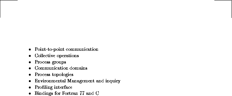
Jack Dongarra
Fri Sep 1 06:16:55 EDT 1995
Probe and Cancel
Next:
Persistent Communication Requests
Up:
Point-to-Point Communication
Previous:
Multiple Completions
pollingcancelationprobing
MPI_PROBE and MPI_IPROBE
allow polling of incoming messages
without
actually receiving them. The application
can then decide how to receive them, based
on the information returned by the probe (in a
status variable). For example, the application might allocate memory for
the receive buffer according to the length of the probed message.
MPI_CANCEL allows pending communications to be canceled.
This is required for cleanup in some situations.
Suppose an application has posted nonblocking sends or receives and
then determines that these operations will not complete.
Posting a send or a receive ties up application resources (send or receive
buffers),
and a cancel allows these resources to be freed.

MPI_Iprobe(int source, int tag, MPI_Comm comm, int *flag, MPI_Status *status)
MPI_IPROBE(SOURCE, TAG, COMM, FLAG, STATUS, IERROR)LOGICAL FLAG
INTEGER SOURCE, TAG, COMM, STATUS(MPI_STATUS_SIZE), IERROR
MPI_IPROBE is a nonblocking operation that
returns flag = true
if there is a message that can be received
and that matches the message envelope specified by
source, tag, and comm.
The call matches the same message
that would have been received by a call to MPI_RECV
(with these arguments)
executed at the same point in the program, and returns in
status the same
value.
Otherwise, the call returns flag = false, and leaves status
undefined.
MPI_IPROBE has local completion semantics.
If MPI_IPROBE(source, tag, comm, flag, status) returns flag = true,
then the first, subsequent receive executed with the
communicator comm, and with the source and tag returned in
status,
will receive the message
that was matched by the probe.
The argument source can be
MPI_ANY_SOURCE, and tag can be
MPI_ANY_SOURCE
MPI_ANY_TAG, so that one can probe for messages from an arbitrary
MPI_ANY_TAG
source and/or with
an arbitrary tag. However, a specific communicator
must be provided in comm.
It is not necessary to receive a message immediately after it has been
probed for, and the
same message may be probed for several times before it is received.

MPI_Probe(int source, int tag, MPI_Comm comm, MPI_Status *status)
MPI_PROBE(SOURCE, TAG, COMM, STATUS, IERROR)INTEGER SOURCE, TAG, COMM, STATUS(MPI_STATUS_SIZE), IERROR
MPI_PROBE behaves like MPI_IPROBE except that it blocks
and returns only after a matching message has been found.
MPI_PROBE has non-local completion semantics.
The semantics of MPI_PROBE and MPI_IPROBE
guarantee progress, in the same way as a corresponding receive executed at the
same point in the program.
progress, for probe
If a call to MPI_PROBE has been issued by a process, and a send that
matches the probe has been initiated by some process, then the call to
MPI_PROBE will return, unless the message is received by another,
concurrent receive operation, irrespective of other activities in the system.
Similarly, if a process busy waits with
MPI_IPROBE and a matching message has been issued,
then the call to
MPI_IPROBE will eventually return flag = true
unless the message is received by another concurrent receive
operation, irrespective of other activities in the system.


MPI_Cancel(MPI_Request *request)
MPI_CANCEL(REQUEST, IERROR)INTEGER REQUEST, IERROR
MPI_CANCEL marks for cancelation a pending,
cancelation
nonblocking communication operation (send or receive). MPI_CANCEL
has local completion semantics.
It returns immediately, possibly before the
communication is actually canceled.
After this, it is still necessary to complete a
communication that has been marked
for cancelation, using a call to MPI_REQUEST_FREE,
MPI_WAIT, MPI_TEST or one of the functions in
Section
. If the communication was not cancelled
(that is, if the communication happened to start before the
cancelation could take effect), then
the completion call will complete the communication, as
usual. If the communication was
successfully cancelled,
then the completion call will deallocate the request object
and will return in status the information that the
communication was canceled.
The application should then call MPI_TEST_CANCELLED,
using status as input, to test
whether the communication was actually canceled.
Either the cancelation succeeds, and no communication occurs, or the
communication completes, and the cancelation fails.
If a send is marked for cancelation, then it must be the case that
either the send completes normally, and the
message sent is received at the destination process, or that the send is
successfully
canceled, and no part of the message is received at the
destination.
If a receive is marked for cancelation, then it must be the case that
either the receive completes normally, or that the receive is
successfully canceled, and no part of the receive buffer
is altered.
If a communication is marked for cancelation, then a completion
call for that communication is guaranteed to return, irrespective of
the activities of other processes. In this case, MPI_WAIT behaves as a
local function. Similarly, if MPI_TEST is
repeatedly called in a busy wait loop for a canceled communication,
then MPI_TEST will eventually succeed.

MPI_Test_cancelled(MPI_Status *status, int *flag)
MPI_TEST_CANCELLED(STATUS, FLAG, IERROR)LOGICAL FLAG
INTEGER STATUS(MPI_STATUS_SIZE), IERROR
MPI_TEST_CANCELLED is used to test whether the communication
operation was actually canceled by MPI_CANCEL.
It returns flag = true if the communication associated with the
status object was canceled successfully. In this case, all
other fields of status are
undefined. It returns flag = false, otherwise.


Next:
Persistent Communication Requests
Up:
Point-to-Point Communication
Previous:
Multiple Completions
Jack Dongarra
Fri Sep 1 06:16:55 EDT 1995
Persistent Communication Requests
Next:
Communication-Complete Calls with
Up:
Point-to-Point Communication
Previous:
Probe and Cancel
persistent requestrequest, persistent
porthalf-channel
Often a communication with the same argument list is repeatedly
executed within the inner loop of a parallel computation. In such a
situation, it may be possible to optimize the communication by
binding the list of communication arguments to a persistent communication
request once and then, repeatedly, using
the request to initiate and complete messages. A
persistent request can be thought of as a
communication port or a ``half-channel.''
It does not provide the full functionality of a conventional channel,
since there is no binding of the send port to the receive port. This
construct allows reduction of the overhead for communication
between the process and communication controller, but not of the overhead for
communication between one communication controller and another.
It is not necessary that messages sent with a persistent request be received
by a receive operation using a persistent request, or vice-versa.
Persistent communication requests are associated with nonblocking
send and receive operations.
A persistent communication request is created using the following
functions. They involve no communication and thus have local
completion semantics.

MPI_Send_init(void* buf, int count, MPI_Datatype datatype, int dest, int tag, MPI_Comm comm, MPI_Request *request)
MPI_SEND_INIT(BUF, COUNT, DATATYPE, DEST, TAG, COMM, REQUEST, IERROR)<type> BUF(*)
INTEGER REQUEST, COUNT, DATATYPE, DEST, TAG, COMM, REQUEST, IERROR
MPI_SEND_INIT
creates a persistent communication request
for a standard-mode, nonblocking send operation, and binds to it all the
arguments of a send operation.

MPI_Recv_init(void* buf, int count, MPI_Datatype datatype, int source, int tag, MPI_Comm comm, MPI_Request *request)
MPI_RECV_INIT(BUF, COUNT, DATATYPE, SOURCE, TAG, COMM, REQUEST, IERROR)<type> BUF(*)
INTEGER COUNT, DATATYPE, SOURCE, TAG, COMM, REQUEST, IERROR
MPI_RECV_INIT
creates a persistent communication request
for a nonblocking receive operation. The
argument buf is marked as OUT
because the application gives permission to write on the receive buffer.
Persistent communication requests are created by the preceding functions,
but they are, so far, inactive. They are activated, and the associated
communication operations started, by MPI_START
or MPI_STARTALL.

MPI_Start(MPI_Request *request)
MPI_START(REQUEST, IERROR)INTEGER REQUEST, IERROR
MPI_START activates request and initiates the
associated communication.
Since all persistent requests are associated with nonblocking
communications, MPI_START has local completion semantics.
The semantics of communications done
with persistent requests are identical to the corresponding
operations without persistent requests.
That is,
a call to MPI_START with a
request created by MPI_SEND_INIT
starts a
communication in the same manner as a call to MPI_ISEND;
a call to MPI_START with a request created by
MPI_RECV_INIT starts a communication in the same manner as
a call to MPI_IRECV.
A send operation initiated with MPI_START can be matched with
any receive operation (including MPI_PROBE)
and a receive operation initiated
with MPI_START can receive messages generated by any send
operation.

MPI_Startall(int count, MPI_Request *array_of_requests)
MPI_STARTALL(COUNT, ARRAY_OF_REQUESTS, IERROR)INTEGER COUNT, ARRAY_OF_REQUESTS(*), IERROR
MPI_STARTALL
starts all communications associated with persistent requests in
array_of_requests. A call to
MPI_STARTALL(count, array_of_requests) has the
same effect as calls to
MPI_START(array_of_requests[i]),
executed for i=0 ,..., count-1, in some arbitrary order.
A communication started with a call to MPI_START or
MPI_STARTALL is
completed by a call to MPI_WAIT, MPI_TEST, or
one of the other completion functions described in
Section
. The persistent request becomes inactive after
the completion of such a call, but it is not deallocated
and it can be re-activated by another MPI_START or
MPI_STARTALL.
Persistent requests are explicitly deallocated by a call to
MPI_REQUEST_FREE (Section
).
The call to MPI_REQUEST_FREE can occur at any point in the program
after the persistent request was created. However, the request will be
deallocated only after it becomes inactive.
Active receive requests should not be freed. Otherwise, it will not be
possible to check that the receive has completed.
It is preferable to free requests when they are inactive. If this
rule is followed, then the functions
described in this section will be invoked
in a sequence of the form,

where  indicates zero or more repetitions.
If the same communication request is used in several concurrent
threads, it is the user's responsibility to coordinate calls so that the
correct sequence is obeyed.
indicates zero or more repetitions.
If the same communication request is used in several concurrent
threads, it is the user's responsibility to coordinate calls so that the
correct sequence is obeyed.
MPI_CANCEL can be used to cancel a communication that uses
a persistent request, in
the same way it is used for nonpersistent requests.
A successful cancelation cancels
the active communication, but does not deallocate the request. After the
call to MPI_CANCEL and the subsequent call to MPI_WAIT or
MPI_TEST (or other completion function), the
request becomes inactive and
can be activated for a new communication.

Next:
Communication-Complete Calls with
Up:
Point-to-Point Communication
Previous:
Probe and Cancel
Jack Dongarra
Fri Sep 1 06:16:55 EDT 1995
Communication-Complete Calls with Null Request Handles
Next:
Communication Modes
Up:
Point-to-Point Communication
Previous:
Persistent Communication Requests
Normally, an invalid handle to an MPI object is not a valid argument for
a call that expects an object. There is one exception to this rule:
communication-complete calls can be passed request handles with value
MPI_REQUEST_NULL.
MPI_REQUEST_NULL
A communication complete call with such an argument is a
``no-op'': the null handles are ignored. The same rule applies to
persistent handles that are not associated with an active
communication operation.
request, null handlenull request handle
request, inactive vs active
active request handle inactive request handle
status, empty
We shall use the following terminology. A null request handle is
a handle with value MPI_REQUEST_NULL. A handle to a
MPI_REQUEST_NULL
persistent request is inactive if the request is not currently
associated with an ongoing communication. A handle is active,
if it is neither null nor inactive.
An empty status is a status
that is set to tag = MPI_ANY_TAG, source =
MPI_ANY_SOURCE, and is also internally configured so that calls to
MPI_ANY_TAG
MPI_ANY_SOURCE
MPI_GET_COUNT and MPI_GET_ELEMENT return
count = 0. We set a status variable to empty in cases
when the value returned is not significant. Status is set this way to
prevent errors due to access of stale information.
A call to MPI_WAIT with a null or inactive request
argument returns immediately with an empty status.
A call to MPI_TEST with a null or inactive request
argument returns immediately with flag = true and an empty status.
The list of requests passed to MPI_WAITANY may contain null or
inactive requests. If some of the requests are active, then the call returns
when an active request has completed. If all the requests in the list
are null or inactive then the call returns immediately, with index =
MPI_UNDEFINED and an empty status.
The list of requests passed to MPI_TESTANY may contain null or
inactive requests. The call returns flag = false if there are
active requests in the list, and none have completed. It returns
flag = true if an active request has completed, or if all the requests
in the list are null or inactive. In the later case, it returns
index = MPI_UNDEFINED and an empty status.
The list of requests passed to MPI_WAITALL may contain null or
inactive requests. The call returns as soon as all active requests
have completed. The call sets to empty each status associated with a
null or inactive request.
The list of requests passed to MPI_TESTALL may contain null or
inactive requests. The call returns flag = true if
all active requests have completed. In this case, the call sets to
empty each status associated with a null or inactive request.
Otherwise, the call returns flag = false.
The list of requests passed to MPI_WAITSOME may contain null or
inactive requests. If the list contains active requests, then the call
returns when some of the active requests have completed. If all requests were
null or inactive,
then the call returns immediately, with outcount = MPI_UNDEFINED.
MPI_UNDEFINED
The list of requests passed to MPI_TESTSOME may contain null or
inactive requests. If the list contains active requests and some have
completed, then the call returns in outcount the number of completed
request. If it contains active requests, and none have completed, then it
returns outcount = 0. If the list contains no active requests, then it
returns outcount = MPI_UNDEFINED.
In all these cases, null or inactive request handles are not modified
by the call.


Next:
Communication Modes
Up:
Point-to-Point Communication
Previous:
Persistent Communication Requests
Jack Dongarra
Fri Sep 1 06:16:55 EDT 1995
Communication Modes
Next:
Blocking Calls
Up:
Point-to-Point Communication
Previous:
Communication-Complete Calls with
modescommunication modes
The send call described in Section
used the standard communication mode. In this mode,
it is up to MPI to decide whether outgoing
messages will be buffered. MPI may
buffer outgoing messages. In such a case, the send call may complete
before a matching receive is invoked. On the other hand, buffer space may be
unavailable, or MPI may choose not to buffer
outgoing messages, for performance reasons. In this case,
the send call will not complete until a matching receive has been posted, and
the data has been moved to the receiver. (A blocking send completes when the
call returns; a nonblocking send completes when the matching Wait or Test call
returns successfully.)
Thus, a send in standard mode can be started whether or not a
matching receive has been posted. It may complete before a matching receive
is posted. The
standard-mode send has non-local completion semantics, since successful
completion of the send
operation may depend on the occurrence of a matching receive.
modecommunication modes
mode, standard
mode, synchronoussynchronous mode
mode, bufferedbuffered mode
mode, readyready mode
standard mode
rendezvous
A buffered-mode send operation can be started whether or not a
matching receive has been posted.
It may complete before a matching receive is posted.
Buffered-mode send has local completion semantics: its
completion does not depend on the occurrence of a matching receive.
In order to complete the operation, it may be necessary to buffer the
outgoing message locally. For that purpose, buffer
space is provided by the application (Section
).
An error will occur if a buffered-mode send is called and
there is insufficient buffer space.
The buffer space occupied by the message is freed when the message is
transferred to its destination or when the buffered send is cancelled.
A synchronous-mode send can be started whether or
not a matching receive was posted. However, the send will complete
successfully only if a matching receive is posted, and the
receive operation has started to receive the message sent by the
synchronous send.
Thus, the completion of a synchronous send not only indicates that the
send buffer can be reused, but also indicates that the receiver has
reached a certain point in its execution, namely that it has started
executing the matching receive. Synchronous mode provides
synchronous communication semantics: a communication does not complete
at either end before both processes rendezvous at the
communication. A synchronous-mode send has non-local completion semantics.
A ready-mode send
may be started only if the matching receive has already been posted.
Otherwise, the operation is erroneous and its outcome is undefined.
On some systems, this allows the removal of a hand-shake
operation and results in improved
performance.
A ready-mode send has the same semantics as a standard-mode send.
In a correct program, therefore, a
ready-mode send could be replaced by a standard-mode send with no effect on the
behavior of the program other than performance.
Three additional send functions are provided for the three additional
communication
modes. The communication mode is indicated by a one letter prefix:
B for buffered,
S for synchronous, and
R for ready.
There is only one receive mode and it matches any of the send modes.
All send and receive operations use the buf, count,
datatype, source, dest, tag,
comm, status and request arguments
in the same way as
the standard-mode send and receive operations.
Next:
Blocking Calls
Up:
Point-to-Point Communication
Previous:
Communication-Complete Calls with
Jack Dongarra
Fri Sep 1 06:16:55 EDT 1995
Blocking Calls
Next:
Nonblocking Calls
Up:
Communication Modes
Previous:
Communication Modes

MPI_Bsend(void* buf, int count, MPI_Datatype datatype, int dest, int tag, MPI_Comm comm)
MPI_BSEND(BUF, COUNT, DATATYPE, DEST, TAG, COMM, IERROR)<type> BUF(*)
INTEGER COUNT, DATATYPE, DEST, TAG, COMM, IERROR
MPI_BSEND performs a buffered-mode, blocking send.

MPI_Ssend(void* buf, int count, MPI_Datatype datatype, int dest, int tag, MPI_Comm comm)
MPI_SSEND(BUF, COUNT, DATATYPE, DEST, TAG, COMM, IERROR)<type> BUF(*)
INTEGER COUNT, DATATYPE, DEST, TAG, COMM, IERROR
MPI_SSEND performs a synchronous-mode, blocking send.

MPI_Rsend(void* buf, int count, MPI_Datatype datatype, int dest, int tag, MPI_Comm comm)
MPI_RSEND(BUF, COUNT, DATATYPE, DEST, TAG, COMM, IERROR)<type> BUF(*)
INTEGER COUNT, DATATYPE, DEST, TAG, COMM, IERROR
MPI_RSEND performs a ready-mode, blocking send.
Jack Dongarra
Fri Sep 1 06:16:55 EDT 1995
Nonblocking Calls
Next:
Persistent Requests
Up:
Communication Modes
Previous:
Blocking Calls
We use the same naming conventions as for blocking communication: a
prefix of B, S, or R is used for buffered,
synchronous or ready mode. In addition, a prefix of I (for
immediate) indicates that the call is nonblocking.
There is only one nonblocking receive call, MPI_IRECV.
Nonblocking send operations are completed with the same Wait and Test
calls as for standard-mode send.

MPI_Ibsend(void* buf, int count, MPI_Datatype datatype, int dest, int tag, MPI_Comm comm, MPI_Request *request)
MPI_IBSEND(BUF, COUNT, DATATYPE, DEST, TAG, COMM, REQUEST, IERROR)<type> BUF(*)
INTEGER COUNT, DATATYPE, DEST, TAG, COMM, REQUEST, IERROR
MPI_IBSEND posts a buffered-mode, nonblocking send.

MPI_Issend(void* buf, int count, MPI_Datatype datatype, int dest, int tag, MPI_Comm comm, MPI_Request *request)
MPI_ISSEND(BUF, COUNT, DATATYPE, DEST, TAG, COMM, REQUEST, IERROR)<type> BUF(*)
INTEGER COUNT, DATATYPE, DEST, TAG, COMM, REQUEST, IERROR
MPI_ISSEND posts a synchronous-mode, nonblocking send.

MPI_Irsend(void* buf, int count, MPI_Datatype datatype, int dest, int tag, MPI_Comm comm, MPI_Request *request)
MPI_IRSEND(BUF, COUNT, DATATYPE, DEST, TAG, COMM, REQUEST, IERROR)<type> BUF(*)
INTEGER COUNT, DATATYPE, DEST, TAG, COMM, REQUEST, IERROR
MPI_IRSEND posts a ready-mode, nonblocking send.
Jack Dongarra
Fri Sep 1 06:16:55 EDT 1995
Persistent Requests
Next:
Buffer Allocation and
Up:
Communication Modes
Previous:
Nonblocking Calls

MPI_Bsend_init(void* buf, int count, MPI_Datatype datatype, int dest, int tag, MPI_Comm comm, MPI_Request *request)
MPI_BSEND_INIT(BUF, COUNT, DATATYPE, DEST, TAG, COMM, REQUEST, IERROR)<type> BUF(*)
INTEGER REQUEST, COUNT, DATATYPE, DEST, TAG, COMM, REQUEST, IERROR
MPI_BSEND_INIT
creates a persistent communication request for a buffered-mode,
nonblocking send,
and binds to it all the
arguments of a send operation.

MPI_Ssend_init(void* buf, int count, MPI_Datatype datatype, int dest, int tag, MPI_Comm comm, MPI_Request *request)
MPI_SSEND_INIT(BUF, COUNT, DATATYPE, DEST, TAG, COMM, REQUEST, IERROR)<type> BUF(*)
INTEGER COUNT, DATATYPE, DEST, TAG, COMM, REQUEST, IERROR
MPI_SSEND_INIT
creates a persistent communication object
for a synchronous-mode, nonblocking send,
and binds to it all the
arguments of a send operation.

MPI_Rsend_init(void* buf, int count, MPI_Datatype datatype, int dest, int tag, MPI_Comm comm, MPI_Request *request)
MPI_RSEND_INIT(BUF, COUNT, DATATYPE, DEST, TAG, COMM, REQUEST, IERROR)<type> BUF(*)
INTEGER COUNT, DATATYPE, DEST, TAG, COMM, REQUEST, IERROR
MPI_RSEND_INIT
creates a persistent communication object
for a ready-mode, nonblocking send,
and binds to it all the
arguments of a send operation.

Jack Dongarra
Fri Sep 1 06:16:55 EDT 1995
Buffer Allocation and Usage
Next:
Model Implementation of
Up:
Communication Modes
Previous:
Persistent Requests
buffered modemode, bufferedbuffer attach
An application must specify a buffer to be used for
buffering messages sent in buffered
mode. Buffering is done by the sender.

MPI_Buffer_attach( void* buffer, int size)
MPI_BUFFER_ATTACH( BUFFER, SIZE, IERROR)<type> BUFFER(*)
INTEGER SIZE, IERROR
MPI_BUFFER_ATTACH
provides to MPI a buffer in the application's
memory to be used for buffering outgoing
messages. The buffer is used only by messages sent in buffered mode.
Only one buffer can be attached at a time (per process).

MPI_Buffer_detach( void* buffer, int* size)
MPI_BUFFER_DETACH( BUFFER, SIZE, IERROR)<type> BUFFER(*)
INTEGER SIZE, IERROR
MPI_BUFFER_DETACH detaches the buffer currently associated
with MPI. The call returns the
address and the size of the detached buffer. This operation
will block until all messages currently in the buffer have been transmitted.
Upon return of
this function, the user may reuse or deallocate the space taken by the buffer.


Now the question arises: how is the attached buffer to be
used? The answer is that MPI must behave
as if
buffer policy
outgoing message
data were buffered by the sending process, in the specified buffer space,
using a circular, contiguous-space allocation policy.
We outline below a model implementation that defines this policy.
MPI may provide more buffering, and may use a better buffer allocation
algorithm
than described below. On the other hand, MPI may signal an error
whenever the
simple buffering allocator described below would run out of space.
Jack Dongarra
Fri Sep 1 06:16:55 EDT 1995
Model Implementation of Buffered Mode
Next:
Comments on Communication
Up:
Communication Modes
Previous:
Buffer Allocation and
The model implementation uses the packing and unpacking functions described in
Section
and the nonblocking communication functions
described in Section
.
We assume that a circular queue
of pending message entries (PME) is maintained. Each
entry contains a communication request
that identifies a pending nonblocking
send, a pointer to the next entry and the packed message data. The
entries are stored in successive locations in the buffer. Free space is
available between the queue tail and the queue head.
A buffered send call results in the execution of the following algorithm.

Jack Dongarra
Fri Sep 1 06:16:55 EDT 1995
Comments on Communication Modes
Next:
User-Defined Datatypes and
Up:
Communication Modes
Previous:
Model Implementation of
mode, comments
communication modes, comments


Jack Dongarra
Fri Sep 1 06:16:55 EDT 1995
What is Not Included in MPI?
Next:
Version of MPI
Up:
Introduction
Previous:
What is Included
MPI does not specify:
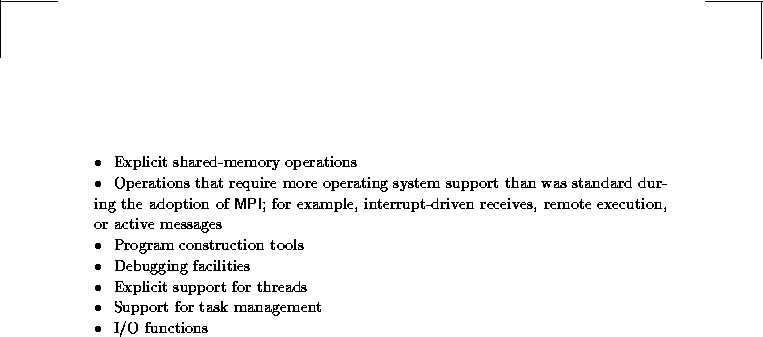
There are many features that were considered and
not included in MPI. This happened for
a number of reasons: the time constraint
that was self-imposed by the MPI Forum in finishing the standard;
the feeling that not enough experience was available on some of these
topics; and the concern that additional features would delay the appearance of
implementations.
Features that are not included can always be offered as extensions
by specific
implementations.
Future versions of MPI will address some of these issues (see
Section
).
Jack Dongarra
Fri Sep 1 06:16:55 EDT 1995
User-Defined Datatypes and Packing
Next:
Introduction
Up:
MPI: The Complete Reference
Previous:
Comments on Communication
Jack Dongarra
Fri Sep 1 06:16:55 EDT 1995
Introduction
Next:
Introduction to User-Defined
Up:
User-Defined Datatypes and
Previous:
User-Defined Datatypes and
The MPI communication mechanisms introduced in the previous chapter
allows one to send or receive a sequence of identical elements that
are contiguous in memory. It is often desirable to send
data that is not homogeneous, such as a structure, or that is
not contiguous in memory, such as an array section. This allows one
to amortize the fixed overhead of sending and receiving a
message over the transmittal of many elements, even in these
more general circumstances. MPI provides two mechanisms to
achieve this.
-
The user can define derived datatypes, that specify more
general data layouts. User-defined datatypes can be used in MPI
communication functions, in place of the basic, predefined datatypes.
derived datatype
-
A sending process can explicitly pack noncontiguous data into a
contiguous buffer, and next send it; a receiving process can explicitly
unpack data received in a contiguous buffer and store in noncontiguous
locations.
packunpack
The construction and use of derived datatypes is described in
Section
-
.
The use of Pack and Unpack functions is described in
Section
. It is often possible to achieve the same
data transfer using either mechanisms. We discuss the pros and cons
of each approach at the end of this chapter.
Jack Dongarra
Fri Sep 1 06:16:55 EDT 1995
Introduction to User-Defined Datatypes
Next:
Datatype Constructors
Up:
User-Defined Datatypes and
Previous:
Introduction
All MPI communication functions take a
datatype argument. In the
simplest case this will be a primitive type, such as an integer or
floating-point number. An important and powerful generalization results
by allowing user-defined (or ``derived'') types wherever the primitive
types can occur. These are not ``types'' as far as the programming
language is concerned. They are only ``types'' in that MPI is made
aware of them through the use of type-constructor functions, and they
describe the layout, in memory, of sets of primitive types. Through
user-defined types, MPI supports the communication of
complex data structures such as array sections and structures containing
combinations of primitive datatypes. Example
shows how
a user-defined datatype is used to send the upper-triangular part
of a matrix, and Figure
diagrams the memory layout
represented by the user-defined datatype.
derived datatypetype constructor
derived datatype, constructor


Figure: A diagram of the memory cells represented by the user-defined
datatype upper. The shaded cells are the locations of the array
that will be sent.
Derived datatypes
are constructed from basic datatypes using the constructors described
in Section
. The constructors can
be applied recursively.
A derived datatype is an opaque object that specifies two
things:

derived datatype
The displacements are not required to be positive, distinct, or
in increasing order. Therefore, the order of items need not
coincide with their order in memory, and an item may appear more than
once.
We call such a pair of sequences (or sequence of pairs) a type map.
The sequence of primitive datatypes (displacements ignored) is the type signature of the datatype.
type maptype signature
derived datatype, mapderived datatype, signature
Let

be such a type map, where  are primitive types, and
 are displacements.
Let
are displacements.
Let

be the associated type signature.
This type map, together with a base address buf,
specifies a communication buffer: the communication buffer that consists of
entries, where the
-th entry is at address  and has type
.
A message assembled from a single type of this sort
will consist of
values, of the types defined
by
and has type
.
A message assembled from a single type of this sort
will consist of
values, of the types defined
by  .
.
A handle to a derived datatype can appear as an argument in a send or
receive operation, instead of a primitive datatype argument. The
operation
MPI_SEND(buf, 1, datatype,...) will use the send buffer
defined by the base address buf and the derived datatype
associated with datatype. It will generate a message with the type
signature determined by the datatype argument.
MPI_RECV(buf, 1, datatype,...) will use the receive buffer
defined by the base address buf and the derived datatype
associated with datatype.
Derived datatypes can be used in all send and receive operations
including collective. We discuss, in
Section
, the case where the second argument
count has value  .
.
The primitive datatypes presented in
Section
are special cases of a derived datatype, and are predefined.
Thus, MPI_INT is a predefined handle to a datatype with type
MPI_INT
map  , with one entry of type int and
displacement zero. The other primitive datatypes are similar.
, with one entry of type int and
displacement zero. The other primitive datatypes are similar.
The extent of a datatype is defined to
be the span from the first byte to the last byte occupied by entries in this
datatype, rounded up to satisfy alignment requirements.
extentderived datatype, extent
That is, if
then

where  .
.  is the lower bound and
  is
the upper bound of the datatype.
lower boundderived datatype, lower bound
upper boundderived datatype, upper bound
If
requires alignment to a byte address that is a multiple
of
is
the upper bound of the datatype.
lower boundderived datatype, lower bound
upper boundderived datatype, upper bound
If
requires alignment to a byte address that is a multiple
of  ,
then
,
then  is the least nonnegative increment needed to round
 to the next multiple of
  .
(The definition of extent is expanded in Section
.)
.
(The definition of extent is expanded in Section
.)


The following functions return information on datatypes.

MPI_Type_extent(MPI_Datatype datatype, MPI_Aint *extent)
MPI_TYPE_EXTENT(DATATYPE, EXTENT, IERROR)INTEGER DATATYPE, EXTENT, IERROR
MPI_TYPE_EXTENT
returns the extent of a datatype. In addition to its use with
derived datatypes, it can be used to inquire about the extent
of primitive datatypes. For example, MPI_TYPE_EXTENT(MPI_INT, extent)
will return in extent the size, in bytes, of an int - the same
value that would be returned by the C call sizeof(int).

extentderived datatype, extent

MPI_Type_size(MPI_Datatype datatype, int *size)
MPI_TYPE_SIZE(DATATYPE, SIZE, IERROR)INTEGER DATATYPE, SIZE, IERROR
MPI_TYPE_SIZE returns the total size, in bytes, of the entries in
the type signature
associated with datatype; that is, the total size of
the data in a message that would be created with this datatype. Entries that
occur multiple times in the datatype are counted with their multiplicity.
For primitive datatypes, this function returns the same information as
MPI_TYPE_EXTENT.

Next:
Datatype Constructors
Up:
User-Defined Datatypes and
Previous:
Introduction
Jack Dongarra
Fri Sep 1 06:16:55 EDT 1995
Datatype Constructors
Next:
Contiguous
Up:
User-Defined Datatypes and
Previous:
Introduction to User-Defined
This section presents the MPI functions for constructing derived
datatypes. The functions are presented in an order from
simplest to most complex.
type constructor
derived datatype, constructor
Jack Dongarra
Fri Sep 1 06:16:55 EDT 1995
Contiguous
Next:
Vector
Up:
Datatype Constructors
Previous:
Datatype Constructors

MPI_Type_contiguous(int count, MPI_Datatype oldtype, MPI_Datatype *newtype)
MPI_TYPE_CONTIGUOUS(COUNT, OLDTYPE, NEWTYPE, IERROR)INTEGER COUNT, OLDTYPE, NEWTYPE, IERROR
MPI_TYPE_CONTIGUOUS is the simplest datatype constructor.
It constructs a typemap consisting of the replication of a
datatype into contiguous locations.
The argument newtype is the datatype obtained by concatenating
count copies of
oldtype. Concatenation is defined using extent(oldtype)
as the size of the concatenated copies.
The action of the Contiguous
constructor is represented schematically in Figure
.

Figure: Effect of datatype constructor MPI_TYPE_CONTIGUOUS.

In general,
assume that the type map of oldtype is

with extent  .
Then newtype has a type map with
.
Then newtype has a type map with  entries
defined by:
entries
defined by:


Jack Dongarra
Fri Sep 1 06:16:55 EDT 1995
Vector
Next:
Hvector
Up:
Datatype Constructors
Previous:
Contiguous

MPI_Type_vector(int count, int blocklength, int stride, MPI_Datatype oldtype, MPI_Datatype *newtype)
MPI_TYPE_VECTOR(COUNT, BLOCKLENGTH, STRIDE, OLDTYPE, NEWTYPE, IERROR)INTEGER COUNT, BLOCKLENGTH, STRIDE, OLDTYPE, NEWTYPE, IERROR
MPI_TYPE_VECTOR is a constructor that
allows replication of a datatype
into locations that consist of equally spaced blocks. Each block
is obtained by concatenating the same number of copies of the old datatype.
The spacing between blocks is a multiple of the extent of the old datatype.
The action of the Vector
constructor is represented schematically in
Figure
.

Figure: Datatype constructor MPI_TYPE_VECTOR.


In general, assume that oldtype has type map
with extent
. Let bl be the blocklength.
The new datatype has a type map with
 entries:


A call to MPI_TYPE_CONTIGUOUS(count, oldtype, newtype) is
equivalent to a call to
MPI_TYPE_VECTOR(count, 1, 1, oldtype, newtype), or to a call to
MPI_TYPE_VECTOR(1, count, num, oldtype, newtype),
with num arbitrary.
Jack Dongarra
Fri Sep 1 06:16:55 EDT 1995
Hvector
Next:
Indexed
Up:
Datatype Constructors
Previous:
Vector
The Vector type constructor assumes that the stride
between successive blocks is a multiple of the oldtype extent. This
avoids, most of the time, the need for computing stride in bytes.
Sometimes it is useful to relax this assumption and allow a stride which
consists of an arbitrary number of bytes.
The Hvector type constructor below achieves this purpose. The usage of both
Vector and Hvector is illustrated in
Examples
-
.

MPI_Type_hvector(int count, int blocklength, MPI_Aint stride, MPI_Datatype oldtype, MPI_Datatype *newtype)
MPI_TYPE_HVECTOR(COUNT, BLOCKLENGTH, STRIDE, OLDTYPE, NEWTYPE, IERROR)INTEGER COUNT, BLOCKLENGTH, STRIDE, OLDTYPE, NEWTYPE, IERROR
MPI_TYPE_HVECTOR is identical to
MPI_TYPE_VECTOR, except that stride is given in bytes,
rather than in elements.
(H stands for ``heterogeneous'').
The action of the Hvector
constructor is represented schematically in
Figure
.

Figure: Datatype constructor MPI_TYPE_HVECTOR.

In general, assume that oldtype has type map
with extent
. Let bl be the blocklength.
The new datatype has a type map with
entries:


Figure: Memory layout of 2D array section for
Example
. The shaded blocks are sent.


Jack Dongarra
Fri Sep 1 06:16:55 EDT 1995
Indexed
Next:
Hindexed
Up:
Datatype Constructors
Previous:
Hvector
The Indexed constructor allows one to specify a noncontiguous data layout where
displacements between successive blocks need not be equal. This
allows one to
gather arbitrary entries from an array and send them in one message, or
receive one message and scatter the received entries into arbitrary
locations in an array.

MPI_Type_indexed(int count, int *array_of_blocklengths, int *array_of_displacements, MPI_Datatype oldtype, MPI_Datatype *newtype)
MPI_TYPE_INDEXED(COUNT, ARRAY_OF_BLOCKLENGTHS, ARRAY_OF_DISPLACEMENTS, OLDTYPE, NEWTYPE, IERROR)INTEGER COUNT, ARRAY_OF_BLOCKLENGTHS(*), ARRAY_OF_DISPLACEMENTS(*), OLDTYPE, NEWTYPE, IERROR
MPI_TYPE_INDEXED allows
replication of an old datatype into a sequence of blocks (each block is
a concatenation of the old datatype), where
each block can contain a different number of copies of oldtype
and have a different
displacement. All block displacements are measured in units of the
oldtype extent.
The action of the Indexed
constructor is represented schematically in
Figure
.

Figure: Datatype constructor MPI_TYPE_INDEXED.

In general,
assume that oldtype has type map
with extent ex.
Let B be the array_of_blocklengths argument and
D be the
array_of_displacements argument. The new datatype
has a type map with  entries:


A call to MPI_TYPE_VECTOR(count, blocklength, stride, oldtype,
newtype) is equivalent to a call to
MPI_TYPE_INDEXED(count, B, D, oldtype, newtype) where

and

The use of the MPI_TYPE_INDEXED function was illustrated in
Example
, on page
; the function was used
to transfer the upper triangular part of a square matrix.
Jack Dongarra
Fri Sep 1 06:16:55 EDT 1995
Hindexed
Next:
Struct
Up:
Datatype Constructors
Previous:
Indexed
As with the Vector and Hvector constructors, it is usually convenient to measure
displacements in multiples of the extent of the oldtype, but sometimes necessary
to allow for arbitrary displacements. The Hindexed constructor satisfies the
later need.

MPI_Type_hindexed(int count, int *array_of_blocklengths, MPI_Aint *array_of_displacements, MPI_Datatype oldtype, MPI_Datatype *newtype)
MPI_TYPE_HINDEXED(COUNT, ARRAY_OF_BLOCKLENGTHS, ARRAY_OF_DISPLACEMENTS, OLDTYPE, NEWTYPE, IERROR)INTEGER COUNT, ARRAY_OF_BLOCKLENGTHS(*), ARRAY_OF_DISPLACEMENTS(*), OLDTYPE, NEWTYPE, IERROR
MPI_TYPE_HINDEXED is identical to
MPI_TYPE_INDEXED, except that block displacements in
array_of_displacements are specified in
bytes, rather than in multiples of the oldtype extent.
The action of the Hindexed
constructor is represented schematically in
Figure
.

Figure: Datatype constructor MPI_TYPE_HINDEXED.

In general, assume that oldtype has type map
with extent
.
Let B be the array_of_blocklength argument and
D be the
array_of_displacements argument. The new datatype
has a type map with
entries:


Jack Dongarra
Fri Sep 1 06:16:55 EDT 1995
Struct
Next:
Use of Derived
Up:
Datatype Constructors
Previous:
Hindexed

MPI_Type_struct(int count, int *array_of_blocklengths, MPI_Aint *array_of_displacements, MPI_Datatype *array_of_types, MPI_Datatype *newtype)
MPI_TYPE_STRUCT(COUNT, ARRAY_OF_BLOCKLENGTHS, ARRAY_OF_DISPLACEMENTS, ARRAY_OF_TYPES, NEWTYPE, IERROR)INTEGER COUNT, ARRAY_OF_BLOCKLENGTHS(*), ARRAY_OF_DISPLACEMENTS(*), ARRAY_OF_TYPES(*), NEWTYPE, IERROR
MPI_TYPE_STRUCT is the most general type constructor.
It further generalizes MPI_TYPE_HINDEXED
in that it allows each block to consist of replications of
different datatypes.
The intent is to allow descriptions of arrays of structures, as a single
datatype.
The action of the Struct
constructor is represented schematically in
Figure
.

Figure: Datatype constructor MPI_TYPE_STRUCT.

In general,
let T be the array_of_types argument, where T[i]
is a handle to,

with extent  .
Let
B be the array_of_blocklength argument and D be
the array_of_displacements argument.
Let c be the
count argument.
Then the new datatype has a type map with
.
Let
B be the array_of_blocklength argument and D be
the array_of_displacements argument.
Let c be the
count argument.
Then the new datatype has a type map with
 entries:


A call to MPI_TYPE_HINDEXED(count, B, D, oldtype, newtype) is
equivalent to a call to
MPI_TYPE_STRUCT(count, B, D, T, newtype), where each entry
of T is equal to oldtype.


Jack Dongarra
Fri Sep 1 06:16:55 EDT 1995
Version of MPI
Next:
MPI Conventions and
Up:
Introduction
Previous:
What is Not
The original MPI standard was created by the Message Passing
Interface Forum (MPIF). The public release of version 1.0 of
MPI was made in June 1994. The MPIF began meeting again in March
1995. One of the first tasks undertaken was to make clarifications
and corrections to the MPI standard. The changes from version 1.0
to version 1.1 of the MPI standard were limited to ``corrections''
that were deemed urgent and necessary. This work was completed in
June 1995 and version 1.1 of the standard was released. This book
reflects the updated version 1.1 of the MPI standard.
Jack Dongarra
Fri Sep 1 06:16:55 EDT 1995
Use of Derived Datatypes
Next:
Commit
Up:
User-Defined Datatypes and
Previous:
Struct
Jack Dongarra
Fri Sep 1 06:16:55 EDT 1995
Commit
Next:
Deallocation
Up:
Use of Derived
Previous:
Use of Derived
A derived datatype must be committed before it can be used in a
communication. A committed datatype can continue to be used as an input argument in
datatype constructors (so that other datatypes can be derived from the
committed datatype).
There is no need to commit primitive datatypes.
derived datatype, commitcommit

MPI_Type_commit(MPI_Datatype *datatype)
MPI_TYPE_COMMIT(DATATYPE, IERROR)INTEGER DATATYPE, IERROR
MPI_TYPE_COMMIT
commits the datatype.
Commit should be thought of as a possible ``flattening'' or ``compilation''
of the formal description of a type map into an efficient representation.
Commit does not imply that the datatype is bound to the
current content of a communication buffer.
After a datatype
has been committed, it can be repeatedly reused to communicate
different data.

Jack Dongarra
Fri Sep 1 06:16:55 EDT 1995
Deallocation
Next:
Relation to count
Up:
Use of Derived
Previous:
Commit
A datatype object is deallocated by a call to MPI_TYPE_FREE.

MPI_Type_free(MPI_Datatype *datatype)
MPI_TYPE_FREE(DATATYPE, IERROR)INTEGER DATATYPE, IERROR
MPI_TYPE_FREE
marks the datatype object associated with datatype for
deallocation and sets datatype to MPI_DATATYPE_NULL.
MPI_DATATYPE_NULL
Any communication that is currently using this datatype will complete normally.
Derived datatypes that were defined from the freed datatype are not
affected.
derived datatype, destructor


Jack Dongarra
Fri Sep 1 06:16:55 EDT 1995
Relation to <i>count</i>
Next:
Type Matching
Up:
Use of Derived
Previous:
Deallocation
A call of the form MPI_SEND(buf, count, datatype , ...), where
 , is interpreted as if the call was passed a new datatype
which is the
concatenation of count copies of datatype.
Thus,
MPI_SEND(buf, count, datatype, dest, tag, comm) is equivalent to,
, is interpreted as if the call was passed a new datatype
which is the
concatenation of count copies of datatype.
Thus,
MPI_SEND(buf, count, datatype, dest, tag, comm) is equivalent to,
MPI_TYPE_CONTIGUOUS(count, datatype, newtype)
MPI_TYPE_COMMIT(newtype)
MPI_SEND(buf, 1, newtype, dest, tag, comm).
Similar statements apply to all other communication functions that have a
count and datatype argument.
Jack Dongarra
Fri Sep 1 06:16:55 EDT 1995
Type Matching
Next:
Message Length
Up:
Use of Derived
Previous:
Relation to count
Suppose that a send operation MPI_SEND(buf, count,
datatype, dest, tag, comm) is executed, where
datatype has type map

and extent  .
type matchingderived datatype, matching
The send
operation sends
.
type matchingderived datatype, matching
The send
operation sends  entries, where entry
  is at location
 and has type
  ,
for
,
for  and
.
The variable stored at address
and
.
The variable stored at address  in the calling program
should be of a type that matches
, where
type matching is defined as in Section
.
in the calling program
should be of a type that matches
, where
type matching is defined as in Section
.
Similarly, suppose that a receive operation
MPI_RECV(buf, count, datatype, source, tag, comm, status) is
executed.
The receive operation receives up to
entries, where entry
is at location
 and has type
.
Type matching is defined according to the type signature of
the corresponding datatypes, that is, the sequence of primitive type
components. Type matching does not depend on other aspects of the
datatype definition, such as the displacements (layout in memory) or the
intermediate types used to define the datatypes.
and has type
.
Type matching is defined according to the type signature of
the corresponding datatypes, that is, the sequence of primitive type
components. Type matching does not depend on other aspects of the
datatype definition, such as the displacements (layout in memory) or the
intermediate types used to define the datatypes.
For sends,
a datatype may specify overlapping entries.
This is not true for receives. If the datatype used in a receive
operation specifies overlapping entries then
the call is erroneous.
derived datatype, overlapping entries

Jack Dongarra
Fri Sep 1 06:16:55 EDT 1995
Message Length
Next:
Address Function
Up:
Use of Derived
Previous:
Type Matching
If a message was received using a user-defined datatype, then a
subsequent call
to MPI_GET_COUNT(status, datatype, count)
(Section
) will
return the number of ``copies'' of
datatype received (count).
That is, if the receive operation was MPI_RECV(buff,
count,datatype,...) then MPI_GET_COUNT
may return any integer value  , where
  .
If MPI_GET_COUNT returns
, then the number of primitive
elements received
is
.
If MPI_GET_COUNT returns
, then the number of primitive
elements received
is  , where
is the number of primitive elements in the type
map of datatype.
The received message need not fill an integral number of ``copies'' of
datatype.
If the number of primitive elements received is not a
multiple of
, that is, if the receive operation has not received an
integral number of datatype ``copies,'' then
MPI_GET_COUNT returns the value MPI_UNDEFINED.
MPI_UNDEFINED
, where
is the number of primitive elements in the type
map of datatype.
The received message need not fill an integral number of ``copies'' of
datatype.
If the number of primitive elements received is not a
multiple of
, that is, if the receive operation has not received an
integral number of datatype ``copies,'' then
MPI_GET_COUNT returns the value MPI_UNDEFINED.
MPI_UNDEFINED
The function MPI_GET_ELEMENTS below can be used to determine
the number of primitive elements received.

MPI_Get_elements(MPI_Status *status, MPI_Datatype datatype, int *count)
MPI_GET_ELEMENTS(STATUS, DATATYPE, COUNT, IERROR)INTEGER STATUS(MPI_STATUS_SIZE), DATATYPE, COUNT, IERROR

The function MPI_GET_ELEMENTS can also be used after a probe
to find the number of primitive datatype elements in the probed message.
Note that the two functions MPI_GET_COUNT and
MPI_GET_ELEMENTS return the same values when they are used
with primitive datatypes.


alignment
Jack Dongarra
Fri Sep 1 06:16:55 EDT 1995
Address Function
Next:
Lower-bound and Upper-bound
Up:
User-Defined Datatypes and
Previous:
Message Length
As shown in Example
,
page
, one sometimes needs to be able to
find the displacement, in bytes, of a structure component relative to the
structure start. In C, one can use the sizeof operator to
find the size of C objects; and one will be tempted to use the
& operator to compute addresses and then displacements.
However, the C standard does not require that (int)& be the
byte address of variable v: the mapping of pointers to
integers is implementation dependent. Some systems may have ``word''
pointers and ``byte'' pointers; other systems may have a segmented,
noncontiguous address space. Therefore, a portable mechanism has to be
provided by MPI to compute the ``address'' of a variable. Such a
mechanism is certainly needed in Fortran, which has no dereferencing
operator.
addressderived datatype, address

MPI_Address(void* location, MPI_Aint *address)
MPI_ADDRESS(LOCATION, ADDRESS, IERROR)<type> LOCATION(*)
INTEGER ADDRESS, IERROR
MPI_ADDRESS is used to find
the address of a location in memory.
It returns the byte address of location.


Jack Dongarra
Fri Sep 1 06:16:55 EDT 1995
Lower-bound and Upper-bound Markers
Next:
Absolute Addresses
Up:
User-Defined Datatypes and
Previous:
Address Function
Sometimes it is necessary to override the definition of
extent given in Section
.
markersderived datatype, markers
Consider, for example, the code in Example
in
the previous section.
Assume that
a double occupies 8 bytes
and must be double-word aligned.
There will be 7 bytes of padding after the first field and one byte of
padding after the last field of the structure Partstruct, and
the structure will occupy 64 bytes.
If, on the other hand, a double can be word aligned
only, then there will be only 3 bytes of padding after the first
field, and Partstruct will occupy 60 bytes.
The MPI library will follow
the alignment rules used on the target systems so that the extent of datatype
Particletype equals the amount of storage occupied by
Partstruct. The catch is that different
alignment rules may be specified, on the same system,
using different compiler options. An even more difficult problem is that
some compilers allow the use of pragmas in order to specify different alignment
rules for different structures within the same program. (Many
architectures can correctly handle misaligned values, but with lower
performance; different alignment rules trade speed of access for storage
density.) The MPI library will assume the default alignment rules. However,
the user should be able to overrule this assumption if structures are packed
otherwise.
alignment
To allow this capability, MPI has
two additional ``pseudo-datatypes,'' MPI_LB and MPI_UB,
MPI_LB
MPI_UB
that can be used, respectively, to mark the lower bound or the upper
bound of a datatype. These pseudo-datatypes occupy no space
( ). They do not
affect the size or count of a datatype, and do not affect the
the content of a message created with this datatype. However, they do
change the extent of a datatype and, therefore, affect the outcome
of a replication of this datatype by a datatype constructor.
). They do not
affect the size or count of a datatype, and do not affect the
the content of a message created with this datatype. However, they do
change the extent of a datatype and, therefore, affect the outcome
of a replication of this datatype by a datatype constructor.

In general, if

then the lower bound of  is defined to be

Similarly,
the upper bound of
is defined to be

And

If
requires alignment to a byte address that is a multiple of
,
then
is the least nonnegative increment needed to round
to the next multiple of
.
The formal definitions given for the various datatype constructors
continue to apply, with the amended definition of extent.
Also, MPI_TYPE_EXTENT returns the above as its value for extent.
extentderived datatype, extent
lower boundderived datatype, lower bound
upper boundderived datatype, upper bound

The two functions below can be used for finding the lower bound and
the upper bound of a datatype.

MPI_Type_lb(MPI_Datatype datatype, MPI_Aint* displacement)
MPI_TYPE_LB(DATATYPE, DISPLACEMENT, IERROR)INTEGER DATATYPE, DISPLACEMENT, IERROR
MPI_TYPE_LB returns the lower bound of a datatype, in bytes,
relative to the datatype origin.

MPI_Type_ub(MPI_Datatype datatype, MPI_Aint* displacement)
MPI_TYPE_UB(DATATYPE, DISPLACEMENT, IERROR)INTEGER DATATYPE, DISPLACEMENT, IERROR
MPI_TYPE_UB returns the upper bound of a datatype, in bytes,
relative to the datatype origin.
Next:
Absolute Addresses
Up:
User-Defined Datatypes and
Previous:
Address Function
Jack Dongarra
Fri Sep 1 06:16:55 EDT 1995
Absolute Addresses
Next:
Pack and Unpack
Up:
User-Defined Datatypes and
Previous:
Lower-bound and Upper-bound
Consider Example
on page
.
One computes the ``absolute address'' of the structure components, using calls
to MPI_ADDRESS, then subtracts the starting address of the array to
compute relative displacements. When the send operation is executed, the
starting address of the array is added back, in order to compute the send buffer
location. These superfluous arithmetics could be avoided if ``absolute''
addresses were used in the derived datatype, and ``address zero'' was
passed as the buffer argument in the send call.
addressderived datatype, address
MPI supports the use of such ``absolute'' addresses in derived datatypes.
The displacement arguments used in datatype constructors can be ``absolute
addresses'', i.e., addresses returned by calls to MPI_ADDRESS.
Address zero is indicated to communication functions by passing the constant
MPI_BOTTOM as the buffer argument. Unlike derived datatypes
MPI_BOTTOM
with relative displacements, the use of ``absolute'' addresses
restricts the use to the specific structure for which it was created.


The use of addresses and displacements in MPI is best understood in
the context of a flat address space. Then, the ``address'' of a location, as
computed by calls to MPI_ADDRESS can be
the regular address of that location (or a shift of it), and integer
arithmetic
on MPI ``addresses'' yields the expected result. However, the use of a
flat address space is not mandated by C or Fortran. Another potential
source of problems is that Fortran INTEGER's may be too short
to store full addresses.
Variables belong
to the same sequential storage if they belong to the same
array,
to the same COMMON block in Fortran, or to the same structure in C.
addressderived datatype, address
sequential storage
Implementations may restrict the
use of addresses so that arithmetic on addresses is confined within
sequential storage.
Namely, in a communication call, either
-
The communication buffer specified by the
MPI_BOTTOM
buff, count and datatype arguments is all within the
same sequential storage.
-
The initial buffer address argument buff is equal to
MPI_BOTTOM, count=1 and all addresses in the type map
of datatype are absolute addresses
of the form v+i, where v is an absolute address computed by
MPI_ADDR, i is an integer displacement, and v+i
is in the same sequential storage as v.

Next:
Pack and Unpack
Up:
User-Defined Datatypes and
Previous:
Lower-bound and Upper-bound
Jack Dongarra
Fri Sep 1 06:16:55 EDT 1995
Pack and Unpack
Next:
Derived Datatypes vs
Up:
User-Defined Datatypes and
Previous:
Absolute Addresses
Some existing communication libraries, such as PVM and Parmacs,
provide pack and unpack functions for sending noncontiguous data. In
packunpack
these, the application explicitly packs data into a contiguous buffer
before sending it, and unpacks it from a contiguous buffer after
receiving it. Derived datatypes, described in the previous sections
of this chapter, allow one, in most cases, to avoid explicit packing
and unpacking. The application specifies the layout of the data to be
sent or received, and MPI directly accesses a noncontiguous buffer
when derived datatypes are used. The pack/unpack routines are
provided for compatibility with previous libraries. Also, they
provide some functionality that is not otherwise available in MPI.
For instance, a message can be received in several parts, where the
receive operation done on a later part may depend on the content of a
former part. Another use is that the availability of pack and unpack
operations facilitates the development of additional communication
libraries layered on top of MPI.
layering

MPI_Pack(void* inbuf, int incount, MPI_Datatype datatype, void *outbuf, int outsize, int *position, MPI_Comm comm)
MPI_PACK(INBUF, INCOUNT, DATATYPE, OUTBUF, OUTSIZE, POSITION, COMM, IERROR)<type> INBUF(*), OUTBUF(*)
INTEGER INCOUNT, DATATYPE, OUTSIZE, POSITION, COMM, IERROR
MPI_PACK
packs a message specified by inbuf, incount, datatype, comm
into the buffer
space specified by outbuf and outsize. The
input buffer can
be any communication buffer allowed in MPI_SEND. The output buffer
is a contiguous storage area containing outsize bytes, starting at
the address outbuf.
The input value of position is the first
position in the output buffer to be used for packing. The argument
position is
incremented by the size of the packed message so that it can be used
as input to a subsequent call to MPI_PACK.
The comm argument
is the communicator that will be subsequently used for sending the packed
message.

MPI_Unpack(void* inbuf, int insize, int *position, void *outbuf, int outcount, MPI_Datatype datatype, MPI_Comm comm)
MPI_UNPACK(INBUF, INSIZE, POSITION, OUTBUF, OUTCOUNT, DATATYPE, COMM, IERROR)<type> INBUF(*), OUTBUF(*)
INTEGER INSIZE, POSITION, OUTCOUNT, DATATYPE, COMM, IERROR
MPI_UNPACK
unpacks a message into the receive buffer specified by
outbuf, outcount, datatype from the buffer
space specified by inbuf and insize. The output buffer can
be any communication buffer allowed in MPI_RECV. The input
buffer is a contiguous storage area containing insize bytes,
starting at address inbuf.
The input value of position is the position in
the input buffer where one wishes the unpacking to begin.
The output value of position is incremented
by the size of the packed message, so that
it can be used as input to a subsequent call
to MPI_UNPACK.
The argument
comm was the communicator used to receive the packed message.


The MPI_PACK/MPI_UNPACK calls relate to message passing as
the sprintf/sscanf calls in C relate to file I/O, or internal
Fortran files relate to external units. Basically, the
MPI_PACK function allows one to ``send'' a message into a
memory buffer; the MPI_UNPACK function allows one to
``receive'' a message from a memory buffer.
Several communication buffers can be successively packed into one packing unit. This
packing unit
is effected by several, successive related calls to MPI_PACK,
where the first
call provides position = 0, and each successive call inputs the value
of position that was output by the previous call, and the same values
for outbuf, outcount and comm. This packing unit
now contains
the equivalent information that would have been stored in a message by one send
call with a send buffer that is the ``concatenation'' of the individual send
buffers.
A packing unit must
be sent using type MPI_PACKED. Any point-to-point
MPI_PACKED
or collective communication function can be used.
The message sent is identical to the message
that would be sent by a send operation with a
datatype argument describing the concatenation of the send
buffer(s) used in the Pack calls. The message
can be received with any datatype that matches this send datatype.

Any message
can be received in a point-to-point or collective communication
using the type MPI_PACKED. Such a message can then be
MPI_PACKED
unpacked by calls to MPI_UNPACK.
The message
can be unpacked by several, successive calls to
MPI_UNPACK, where the first
call provides position = 0, and each successive call inputs the value
of position that was output by the previous call, and the same values
for inbuf, insize and comm.


MPI_Pack_size(int incount, MPI_Datatype datatype, MPI_Comm comm, int *size)
MPI_PACK_SIZE(INCOUNT, DATATYPE, COMM, SIZE, IERROR)INTEGER INCOUNT, DATATYPE, COMM, SIZE, IERROR
MPI_PACK_SIZE
allows the application to find out how much space is
needed to pack a message and, thus, manage space allocation for
buffers. The function
returns, in size, an upper bound on the increment in position
that would occur in a call to MPI_PACK with the same values
for incount, datatype, and comm.


Next:
Derived Datatypes vs
Up:
User-Defined Datatypes and
Previous:
Absolute Addresses
Jack Dongarra
Fri Sep 1 06:16:55 EDT 1995
MPI Conventions and Design Choices
Next:
Document Notation
Up:
Introduction
Previous:
Version of MPI
This section explains notational terms and conventions used
throughout this book.
Jack Dongarra
Fri Sep 1 06:16:55 EDT 1995
Derived Datatypes vs Pack/Unpack
Next:
Collective Communications
Up:
Pack and Unpack
Previous:
Pack and Unpack
A comparison between Example
on page
and
Example
in the previous section is instructive.
First, programming
convenience. It is somewhat less tedious to pack the class zero particles
in the loop that locates them, rather then defining in this loop the
datatype that will later collect them. On the other hand, it would be
very tedious (and inefficient) to pack separately the components of
each structure entry in the array. Defining a datatype is more convenient
when this definition depends only on declarations; packing may be more
convenient when the communication buffer layout is data dependent.
Second, storage use. The packing code uses at least 56,000 bytes for the
pack buffer, e.g., up to 1000 copies of the structure (1 char, 6
doubles, and 7 char is  bytes).
The derived datatype code uses 12,000
bytes for the three, 1,000 long, integer
arrays used to define the derived datatype.
It also probably uses a similar amount of
storage for the internal datatype representation. The difference is
likely to be larger in realistic codes. The use of packing
requires additional storage for a copy
of the data, whereas the use of derived
datatypes requires additional storage for a description of the
data layout.
bytes).
The derived datatype code uses 12,000
bytes for the three, 1,000 long, integer
arrays used to define the derived datatype.
It also probably uses a similar amount of
storage for the internal datatype representation. The difference is
likely to be larger in realistic codes. The use of packing
requires additional storage for a copy
of the data, whereas the use of derived
datatypes requires additional storage for a description of the
data layout.
Finally, compute time. The packing code executes a function call for
each packed item whereas the derived datatype code executes only a fixed
number of function calls. The packing code is likely to require one
additional memory to memory copy of the data, as compared to the
derived-datatype code. One may expect, on most implementations, to
achieve better performance with the derived datatype code.
Both codes send the same size message, so that there is no
difference in
communication time.
However, if the buffer
described by the derived datatype is
not contiguous
in memory, it may take longer to access.
Example
above illustrates another advantage of
pack/unpack; namely the receiving process may use information in part
of an incoming message in order to decide how to handle subsequent
data in the message. In order to achieve the same outcome without
pack/unpack, one would have to send two messages: the first with the
list of indices, to be used to construct a derived datatype that is
then used to receive the particle entries sent in a second message.
The use of derived datatypes will often lead to improved performance:
data copying can be avoided, and information on data layout can be
reused, when the same communication buffer is reused. On the other
hand, the definition of derived datatypes for complex layouts can be
more tedious than explicit packing.
Derived datatypes should be used whenever data layout is defined by program
declarations (e.g., structures), or is regular (e.g., array sections).
Packing might be considered for complex, dynamic, data-dependent
layouts. Packing may result in more efficient code in situations
where the sender has to communicate to the receiver
information that affects the layout of the receive buffer.
Next:
Collective Communications
Up:
Pack and Unpack
Previous:
Pack and Unpack
Jack Dongarra
Fri Sep 1 06:16:55 EDT 1995
Collective Communications
Next:
Introduction and Overview
Up:
MPI: The Complete Reference
Previous:
Derived Datatypes vs
Jack Dongarra
Fri Sep 1 06:16:55 EDT 1995
Introduction and Overview
Next:
Operational Details
Up:
Collective Communications
Previous:
Collective Communications
Collective communications transmit data among all processes
in a group specified by an intracommunicator object.
One function, the barrier,
serves to synchronize processes without passing data.
MPI provides the following collective communication functions.
collective communicationsynchronization


Figure: Collective move functions illustrated
for a group of six processes. In each case, each row of boxes
represents data locations in one process. Thus, in the broadcast,
initially just the first process contains the item  , but after the
broadcast all processes contain it.
, but after the
broadcast all processes contain it.
Figure
gives a pictorial representation of the
global communication functions. All these functions (broadcast
excepted) come in two variants: the simple variant, where all
communicated items are messages of the same size, and the ``vector''
variant, where each item can be of a different size. In addition, in
the simple variant, multiple items originating from the same process
or received at the same process, are contiguous in memory; the vector
variant allows to pick the distinct items from non-contiguous
locations.
collective, vector variants
Some of these functions, such as broadcast or gather, have a single
origin or a single receiving process. Such a process is called the
root.
root
Global communication functions basically comes in
three patterns:
-
Root sends data to all processes (itself included): broadcast and
scatter.
-
Root receives data from all processes (itself included): gather.
-
Each process communicates with each process (itself included):
allgather and alltoall.
The syntax and semantics of the MPI collective functions was
designed to be consistent with point-to-point communications.
collective, compatibility with point-to-point
However, to keep the number of functions and their argument lists
to a reasonable level of complexity, the MPI committee made
collective functions more
restrictive than the point-to-point functions, in several ways. One
collective, restrictions
restriction is that, in contrast to point-to-point communication,
the amount of data
sent must exactly match the amount of data specified by the receiver.
A major simplification is that collective functions come in blocking
versions only. Though a standing joke at committee meetings concerned
the ``non-blocking barrier,'' such functions can be quite useful
 and may be included in a future version of MPI.
collective, and blocking semanticsblocking
and may be included in a future version of MPI.
collective, and blocking semanticsblocking
Collective functions do not use a tag argument. Thus, within
each intragroup communication domain, collective calls are matched
strictly according to the order of execution.
tagcollective, and message tag
A final simplification of collective functions concerns modes. Collective
collective, and modesmodes
functions come in only one mode, and this mode may be regarded as
analogous to the standard mode of point-to-point. Specifically, the
semantics are as follows. A collective function (on a given process)
can return as soon as its participation in the overall communication
is complete. As usual, the completion indicates that the caller is now
free to access and modify locations in the communication buffer(s).
It does not indicate that other processes have completed, or even started,
the operation. Thus, a collective communication may, or may not, have
the effect of synchronizing all calling processes. The barrier, of course,
is the exception to this statement.
This choice of semantics was made so as to allow a variety of implementations.
The user of MPI must keep these issues in mind. For example, even
though a particular implementation of MPI may provide a broadcast with the
side-effect of synchronization (the standard allows this), the standard
does not require this, and hence, any program that relies on the
synchronization will be non-portable. On the other hand, a correct and
portable program must allow a collective function to be synchronizing.
Though one should not rely on synchronization side-effects, one must
program so as to allow for it.
portabilitycorrectness
collective, and portabilitycollective, and correctness
Though these issues and statements may seem unusually obscure, they are
merely a consequence of the desire of MPI to:
-
allow efficient implementations on a variety of architectures; and,
-
be clear about exactly what is, and what is not, guaranteed by the standard.
Next:
Operational Details
Up:
Collective Communications
Previous:
Collective Communications
Jack Dongarra
Fri Sep 1 06:16:55 EDT 1995
Operational Details
Next:
Communicator Argument
Up:
Collective Communications
Previous:
Introduction and Overview
A collective operation is executed by having all processes in the group
call the communication routine, with matching arguments.
The syntax and semantics of the collective operations are
defined to be consistent with the syntax and semantics of the
point-to-point operations. Thus, user-defined datatypes are allowed
and must match between sending and receiving processes as specified
in Chapter
.
One of the key arguments is an intracommunicator that defines the group
of participating processes and provides
a communication domain for the operation.
In calls where a root process is defined,
some arguments are specified as
``significant only at root,'' and are ignored for all
participants except the root.
The reader is referred to Chapter
for information concerning communication buffers and type matching rules,
to Chapter
for
user-defined datatypes, and to
Chapter
for information on how to define groups and
create communicators.
The type-matching conditions for the collective operations are more
strict than the corresponding conditions between sender and receiver
in point-to-point. Namely, for collective operations,
the amount of data sent must exactly
match the amount of data specified by the receiver.
Distinct type maps (the layout in memory, see Section
)
between sender and receiver are still allowed.
type matchingcollective, and type matching
Collective communication calls may use the same
communicators as point-to-point communication; MPI guarantees that
messages generated on behalf of collective communication calls will not
be confused with messages generated by point-to-point communication.
A more detailed discussion of correct use of collective
routines is found in Section
.


Jack Dongarra
Fri Sep 1 06:16:55 EDT 1995
Communicator Argument
Next:
Barrier Synchronization
Up:
Collective Communications
Previous:
Operational Details
The key concept of the collective functions is to have a ``group''
communicator, and collectivegroup, for collective
collective, and communicatorcollective, process group
of participating processes. The routines do not have a group
identifier as an explicit argument. Instead, there is a communicator
argument. For the purposes of this chapter, a communicator can be
thought of as a group identifier linked with a communication
domain. An intercommunicator, that is, a communicator that spans two
groups, is not allowed as an argument to a collective function.
intercommunicator, and collective
collective, and intercommunicator
Jack Dongarra
Fri Sep 1 06:16:55 EDT 1995
Barrier Synchronization
Next:
Broadcast
Up:
Collective Communications
Previous:
Communicator Argument
synchronizationbarrier

MPI_Barrier(MPI_Comm comm)
MPI_BARRIER(COMM, IERROR) INTEGER COMM, IERROR
MPI_BARRIER blocks the caller until all group members have called
it. The call returns at any process only after all group members have
entered the call.
Jack Dongarra
Fri Sep 1 06:16:55 EDT 1995
Broadcast
Next:
Example Using MPI_BCAST
Up:
Collective Communications
Previous:
Barrier Synchronization
broadcast

MPI_Bcast(void* buffer, int count, MPI_Datatype datatype, int root, MPI_Comm comm )
MPI_BCAST(BUFFER, COUNT, DATATYPE, ROOT, COMM, IERROR) <type> BUFFER(*)
INTEGER COUNT, DATATYPE, ROOT, COMM, IERROR
MPI_BCAST broadcasts a message from
the process with rank root to all processes
of the group.
The argument root must have identical values on all
processes, and comm must represent the same intragroup
communication domain.
On return, the contents of root's communication buffer
has been copied to all processes.
General, derived datatypes are allowed for datatype.
The type signature of count and datatype on any process must
be equal to the type signature of count and datatype at the root.
This implies that the amount of data sent must be equal to the amount received,
pairwise between each process and the root.
MPI_BCAST and all other data-movement collective routines
make this restriction.
Distinct type maps between sender and receiver are still allowed.
Jack Dongarra
Fri Sep 1 06:16:55 EDT 1995
Example Using MPI_BCAST
Next:
Gather
Up:
Broadcast
Previous:
Broadcast


Jack Dongarra
Fri Sep 1 06:16:55 EDT 1995
Gather
Next:
Examples Using MPI_GATHER
Up:
Collective Communications
Previous:
Example Using MPI_BCAST
gather

MPI_Gather(void* sendbuf, int sendcount, MPI_Datatype sendtype, void* recvbuf, int recvcount, MPI_Datatype recvtype, int root, MPI_Comm comm)
MPI_GATHER(SENDBUF, SENDCOUNT, SENDTYPE, RECVBUF, RECVCOUNT, RECVTYPE, ROOT, COMM, IERROR) <type> SENDBUF(*), RECVBUF(*)
INTEGER SENDCOUNT, SENDTYPE, RECVCOUNT, RECVTYPE, ROOT, COMM, IERROR
Each process (root process included) sends the contents of its send
buffer to the root process. The root process receives the messages and
stores them in rank order.
The outcome is as if each of the n processes in the group
(including the root process) had executed a call to
MPI_Send(sendbuf, sendcount, sendtype, root, ...),
and the
root had executed n calls to
MPI_Recv(recvbuf+i
recvcount
extent(recvtype), recvcount, recvtype, i ,...),
where extent(recvtype) is the type extent obtained from a call to
MPI_Type_extent().
An alternative description is that the n messages sent by the
processes in the group are concatenated in rank order, and the
resulting message is received by the root as if by a call to
MPI_RECV(recvbuf, recvcount
n, recvtype, ...).
The receive buffer is ignored for all non-root processes.
General, derived datatypes are allowed for both sendtype
and recvtype.
The type signature of sendcount and sendtype on process i
must be equal to the type signature of
recvcount and recvtype at the root.
This implies that the amount of data sent must be equal to the
amount of data received, pairwise between each process and the root.
Distinct type maps between sender and receiver are still allowed.
All arguments to the function are significant on process root,
while on other processes, only arguments sendbuf, sendcount,
sendtype, root, and comm are significant.
The argument root
must have identical values on all processes and comm must
represent the same intragroup communication domain.
The specification of counts and types
should not cause any location on the root to be written more than
once. Such a call is erroneous.
Note that the recvcount argument at the root indicates
the number of items it receives from each process, not the total number
of items it receives.
Next:
Examples Using MPI_GATHER
Up:
Collective Communications
Previous:
Example Using MPI_BCAST
Jack Dongarra
Fri Sep 1 06:16:55 EDT 1995
Examples Using MPI_GATHER
Next:
GatherVector Variant
Up:
Gather
Previous:
Gather


Figure: The root process gathers 100 ints from each process
in the group.

Jack Dongarra
Fri Sep 1 06:16:55 EDT 1995
MPI: The Complete Reference


Next:
Contents
7
Scientific and Engineering ComputationJanusz Kowalik, Editor
Data-Parallel Programming on MIMD Computersby Philip J. Hatcher and Michael J. Quinn, 1991
Unstructured Scientific Computation on Scalable Multiprocessorsedited by Piyush Mehrotra, Joel Saltz, and Robert Voigt, 1991
Parallel Computational Fluid Dynamics: Implementations and Resultsedited by Horst D. Simon, 1992
Enterprise Integration Modeling: Proceedings of the First International
Conferenceedited by Charles J. Petrie, Jr., 1992
The High Performance Fortran Handbookby Charles H. Koelbel,
David B. Loveman,
Robert S. Schreiber,
Guy L. Steele Jr. and
Mary E. Zosel, 1993
Using MPI: Portable Parallel Programming with the Message-Passing
Interfaceby William Gropp, Ewing Lusk, and Anthony Skjellum, 1994
PVM: Parallel Virtual Machine-A User's Guide and Tutorial for
Network Parallel Computingby Al Geist, Adam Beguelin, Jack Dongarra, Weicheng Jiang, Bob Manchek,
and Vaidy Sunderam, 1994
Enabling Technologies for Petaflops Computingby Thomas Sterling, Paul Messina, and Paul H. Smith
An Introduction to High-Performance Scientific Computingby Lloyd D. Fosdick, Elizabeth R. Jessup, Carolyn J.C. Schauble,
and Gitta Domik
Practical Parallel Programmingby Gregory V. Wilson
MPI: The Complete Referenceby Marc Snir, Steve Otto, Steven Huss-Lederman, David Walker, and
Jack Dongarra
1996 Massachusetts Institute of Technology
All rights reserved. No part of this book may be reproduced
in any form by any electronic or mechanical means (including
photocopying, recording, or information storage and retrieval)
without permission in writing from the publisher.
Parts of this book came from, ``MPI: A Message-Passing Interface
Standard'' by the Message Passing Interface Forum. That document is
copyrighted by the University of Tennessee. These sections were
copied by permission of the University of Tennessee.
This book was set in LaTeX by the authors and was
printed and bound in the United States of America.
Library of Congress Cataloging-in-Publication Data
Jack Dongarra
Fri Sep 1 06:16:55 EDT 1995
MPI: The Complete Reference

MPI: The Complete Reference
Next:
Contents
Scientific and Engineering ComputationJanusz Kowalik, Editor
Data-Parallel Programming on MIMD Computersby Philip J. Hatcher and Michael J. Quinn, 1991
Unstructured Scientific Computation on Scalable Multiprocessorsedited by Piyush Mehrotra, Joel Saltz, and Robert Voigt, 1991
Parallel Computational Fluid Dynamics: Implementations and Resultsedited by Horst D. Simon, 1992
Enterprise Integration Modeling: Proceedings of the First International
Conferenceedited by Charles J. Petrie, Jr., 1992
The High Performance Fortran Handbookby Charles H. Koelbel,
David B. Loveman,
Robert S. Schreiber,
Guy L. Steele Jr. and
Mary E. Zosel, 1993
Using MPI: Portable Parallel Programming with the Message-Passing
Interfaceby William Gropp, Ewing Lusk, and Anthony Skjellum, 1994
PVM: Parallel Virtual Machine-A User's Guide and Tutorial for
Network Parallel Computingby Al Geist, Adam Beguelin, Jack Dongarra, Weicheng Jiang, Bob Manchek,
and Vaidy Sunderam, 1994
Enabling Technologies for Petaflops Computingby Thomas Sterling, Paul Messina, and Paul H. Smith
An Introduction to High-Performance Scientific Computingby Lloyd D. Fosdick, Elizabeth R. Jessup, Carolyn J.C. Schauble,
and Gitta Domik
Practical Parallel Programmingby Gregory V. Wilson
MPI: The Complete Referenceby Marc Snir, Steve Otto, Steven Huss-Lederman, David Walker, and
Jack Dongarra
1996 Massachusetts Institute of Technology
All rights reserved. No part of this book may be reproduced
in any form by any electronic or mechanical means (including
photocopying, recording, or information storage and retrieval)
without permission in writing from the publisher.
Parts of this book came from, ``MPI: A Message-Passing Interface
Standard'' by the Message Passing Interface Forum. That document is
copyrighted by the University of Tennessee. These sections were
copied by permission of the University of Tennessee.
This book was set in LaTeX by the authors and was
printed and bound in the United States of America.
Library of Congress Cataloging-in-Publication Data
This book is also available in postscript and html forms over the Internet.
To retrieve the postscript file you can use one of the following methods:
- anonymous ftp
- ftp ftp.netlib.org
- cd utk/papers/mpi-book
- get mpi-book.ps
- quit
-
from any machine on the Internet type:
- rcp anon@anonrcp.netlib.org:utk/papers/mpi-book/mpi-book.ps mpi-book.ps
- sending email to
netlib@netlib.org and in the message type:
send mpi-book.ps from utk/papers/mpi-book
To view the html file use the URL:
To order from the publisher, send email to mitpress-orders@mit.edu,
or telephone 800-356-0343 or 617-625-8569. Send snail mail orders to
- The MIT Press
- Book Order Department
- 55 Hayward Street
- Cambridge, MA 02142.
8 x 9 * ??? pages * $??.?? * Original in Paperback ISBN 95-80471
For more information, contact Gita Manaktala, manak@mit.edu.
or
-
Click here
Jack Dongarra
Fri Sep 1 06:16:55 EDT 1995
Contents
Next:
A Bit of
Up:
PVM: Parallel Virtual Machine
Previous:
PVM: Parallel Virtual Machine
Series Foreword
The world of modern computing potentially offers many helpful methods
and tools to scientists and engineers, but the fast pace of change in
computer hardware, software, and algorithms often makes practical use of
the newest computing technology difficult. The Scientific and
Engineering Computation series focuses on rapid advances in computing
technologies and attempts to facilitate transferring these technologies
to applications in science and engineering. It will include books on
theories, methods, and original applications in such areas as
parallelism, large-scale simulations, time-critical computing,
computer-aided design and engineering, use of computers in
manufacturing, visualization of scientific data, and human-machine
interface technology.
The series will help scientists and engineers to understand the current
world of advanced computation and to anticipate future developments that
will impact their computing environments and open up new capabilities
and modes of computation.
This volume presents a software package for developing
parallel programs executable on networked Unix computers.
The tool called Parallel Virtual Machine (PVM) allows a
heterogeneous collection of workstations and
supercomputers to function as a single high-performance
parallel machine. PVM is portable and runs on a wide
variety of modern platforms.
It has been well accepted by the global computing
community and used successfully for solving
large-scale problems in science, industry, and business.
Janusz S. Kowalik
Preface
In this book we describe the
Parallel Virtual Machine
(PVM) system and how to develop programs
using PVM.
PVM is a software system that permits a heterogeneous collection
of Unix computers networked together to be viewed
by a user's program as a single
parallel computer.
PVM is the mainstay of the Heterogeneous Network Computing
research project, a collaborative venture between
Oak Ridge National Laboratory,
the University of Tennessee,
Emory University,
and
Carnegie Mellon University.
The PVM system has evolved in the past several
years into a viable technology for distributed and
parallel processing in a variety of disciplines. PVM supports a
straightforward but functionally complete message-passing model.
PVM is designed to link computing resources and provide users
with a parallel platform for running their computer applications,
irrespective of the number of different computers
they use and where the computers are located.
When
PVM is correctly installed, it is capable of harnessing
the combined resources of typically
heterogeneous networked computing platforms to deliver high levels
of performance and functionality.
In this book, we describe the
architecture of the PVM system and discuss its computing model;
the programming interface it supports;
auxiliary facilities for process groups;
the use of PVM on highly parallel systems
such as the Intel Paragon, Cray T3D, and Thinking Machines CM-5;
and some of the internal
implementation techniques employed. Performance
issues, dealing primarily with communication overheads, are
analyzed, and recent findings as well as enhancements
are presented.
To demonstrate the viability of PVM for large-scale scientific
supercomputing, we also provide some example programs.
This book is not a textbook; rather, it is meant to provide a fast entrance
to the world of heterogeneous network computing.
We intend this book to be used by two groups of readers:
students and researchers working with networks of computers.
As such, we hope this book can serve both as a reference
and as a supplement to a teaching text on aspects of network computing.
This guide will familiarize readers with the basics of PVM and
the concepts used in programming on a network.
The information provided here will help with the following PVM tasks:
-
Writing a program in PVM
-
Building PVM on a system
-
Starting PVM on a set of machines
-
Debugging a PVM application
Next:
A Bit of
Up:
PVM: Parallel Virtual Machine
Previous:
PVM: Parallel Virtual Machine
Footnotes
- ...
- Currently,
the pvmd generates an acknowledgement packet for each data packet.
- ...
- This was once implemented,
but was removed while the code was updated
and hasn't been reintroduced.
Jack Dongarra
Thu Sep 15 21:00:17 EDT 1994
Trends in Distributed Computing
Next:
PVM Overview
Up:
Introduction
Previous:
Heterogeneous Network Computing
Stand-alone workstations delivering several tens of millions of operations
per second are commonplace, and continuing increases in power
are predicted.
When these computer systems are interconnected by an appropriate
high-speed network, their combined computational power
can be applied to solve a variety of
computationally intensive applications.
Indeed,
network computing may even provide supercomputer-level computational power.
Further,
under the right circumstances, the network-based approach can be effective
in coupling several similar multiprocessors, resulting in a configuration
that might be economically and technically difficult to achieve with
supercomputer hardware.
To be effective, distributed computing requires high communication speeds.
In the past fifteen years or so, network speeds have increased by several orders
of magnitude (see Figure
).
Figure: Networking speeds
Among the most notable
advances in computer networking technology
are the following:
-
Ethernet
- the name given to the popular local area packet-switched network
technology invented by Xerox PARC. The Ethernet is a 10 Mbit/s broadcast bus
technology with distributed access control.
-
FDDI
- the Fiber Distributed Data Interface. FDDI is a 100-Mbit/sec token-passing
ring that uses optical fiber for transmission between stations and has dual
counter-rotating rings to provide redundant data paths for reliability.
-
HiPPI
- the high-performance parallel interface. HiPPI is a copper-based
data communications standard capable of transferring data at
800 Mbit/sec over 32 parallel lines or 1.6 Gbit/sec over 64 parallel lines.
Most commercially available high-performance computers offer a
HIPPI interface.
It is a point-to-point channel that does not support multidrop configurations.
-
SONET
- Synchronous Optical Network. SONET is a series of optical signals
that are multiples of a basic signal rate of 51.84 Mbit/sec called OC-1.
The OC-3 (155.52 Mbit/sec) and OC-12 (622.08 Mbit/sec) have been
designated as the customer access rates in future B-ISDN networks,
and signal rates of OC-192 (9.952 Gbit/sec) are defined.
-
ATM
- Asynchronous Transfer Mode. ATM is the technique for transport,
multiplexing, and switching that provides a high
degree of flexibility required by B-ISDN.
ATM is a connection-oriented protocol
employing fixed-size packets
with a 5-byte header and 48 bytes of information.
These advances in high-speed networking
promise high throughput with low latency and make it possible
to utilize distributed computing for years to come.
Consequently,
increasing numbers of universities, government and industrial
laboratories, and financial firms are turning to
distributed computing to solve their computational problems.
The objective of PVM is to enable these institutions
to use distributed computing efficiently.
Next:
PVM Overview
Up:
Introduction
Previous:
Heterogeneous Network Computing
Libpvm<A NAME=1386>
</A>
Next:
Direct Message Routing
Up:
Message Routing
Previous:
Pvmd and Foreign
Four functions
handle all packet traffic into and out of libpvm.
mroute()
is called by higher-level functions
such as pvm_send() and pvm_recv()
to copy messages into and out of the task.
It establishes any necessary routes before calling mxfer().
mxfer()
polls for messages,
optionally blocking until one is received
or until a specified timeout.
It calls mxinput() to copy
fragments into the task and reassemble messages.
In the generic version of PVM,
mxfer()
uses select() to poll all routes (sockets) in order to find
those ready for input or output.
pvmmctl()
is called by mxinput()
when a control message (Section
)
is received.
Direct Message Routing<A NAME=1398>
</A>
Next:
Multicasting
Up:
Libpvm
Previous:
Libpvm
Direct routing allows one task to send messages to another
through a TCP link,
avoiding the overhead of forwarding through the pvmds.
It is implemented entirely in libpvm,
using the notify and control message facilities.
By default,
a task routes messages to its pvmd,
which forwards them on.
If direct routing is enabled
(PvmRouteDirect)
when a message (addressed to a task)
is passed to mroute(),
it attempts to create a direct route if one
doesn't already exist.
The route may be granted or refused by the destination task,
or fail (if the task doesn't exist).
The message is then passed to mxfer().
Libpvm maintains a protocol control block (struct ttpcb)
for each active or denied connection,
in list ttlist.
The state diagram for a ttpcb is shown in
Figure
.
To request a connection,
mroute()
makes a ttpcb and socket,
then
sends a
TC_CONREQ
control message to the destination via the default route.
At the same time,
it sends a TM_NOTIFY message to the pvmd,
to be notified if the destination task exits,
with closure (message tag)
TC_TASKEXIT.
Then it
puts the ttpcb in
state TTCONWAIT,
and calls
mxfer() in blocking mode repeatedly
until the state changes.
When the
destination task
enters
mxfer()
(for example, to receive a message),
it receives the TC_CONREQ message.
The request is granted
if its routing policy (pvmrouteopt != PvmDontRoute)
and implementation
allow a direct connection,
it has resources available,
and the protocol version (TDPROTOCOL) in the request
matches its own.
It makes a ttpcb with state TTGRNWAIT,
creates and listens on a socket,
and
then replies with a TC_CONACK message.
If the destination denies the connection,
it nacks, also with a TC_CONACK message.
The originator receives the TC_CONACK
message,
and either opens the connection (state = TTOPEN) or marks the route denied
(state = TTDENY).
Then, mroute() passes the original message to mxfer(),
which sends it.
Denied connections are cached in order to prevent repeated
negotiation.
If the destination doesn't exist,
the TC_CONACK message never arrives because the TC_CONREQ message is
silently dropped.
However,
the TC_TASKEXIT message generated by the notify system
arrives in its place,
and the ttpcb state is set to TTDENY.
This connect scheme also works if both ends try to
establish a connection at the same time.
They both enter
TTCONWAIT, and
when they receive each other's TC_CONREQ messages,
they go directly to the TTOPEN state.
Figure: Task-task connection state diagram
Next:
Multicasting
Up:
Libpvm
Previous:
Libpvm
Multicasting<A NAME=1436>
</A>
Next:
Task Environment
Up:
Message Routing
Previous:
Direct Message Routing
The libpvm function
pvm_mcast()
sends a message to multiple destinations simultaneously.
The current implementation
only routes multicast messages through the pvmds.
It
uses a 1:N fanout
to ensure that failure of a host doesn't
cause the loss of any messages (other than ones to
that host).
The packet routing layer of the pvmd cooperates with the
libpvm to multicast a message.
To form a multicast address TID (GID)
,
the G bit is set
(refer to Figure
).
The L field is assigned by a counter that is incremented for
each multicast,
so
a new multicast address is used for each message,
then recycled.
To initiate a multicast,
the task sends a TM_MCA message to its pvmd,
containing a list of recipient TIDs.
The pvmd creates a multicast descriptor (struct mca) and GID.
It
sorts the addresses,
removes bogus ones, and duplicates and
caches them in the mca.
To
each destination pvmd
(ones with destination tasks),
it sends a
DM_MCA message with the GID and
destinations on that host.
The GID is sent back to the task in the TM_MCA reply message.
The task sends the multicast message
to the pvmd,
addressed to the GID.
As each packet arrives,
the routing layer
copies it
to each local task
and foreign pvmd.
When a multicast packet arrives at a destination pvmd,
it is copied to each destination task.
Packet order
is preserved,
so
the multicast address and data packets
arrive in order at each destination.
As it forwards multicast
packets,
each pvmd eavesdrops on the header flags.
When it sees a packet with EOM flag set,
it
flushes the mca.
Task Environment
Next:
Environment Variables
Up:
How PVM Works
Previous:
Multicasting
Environment Variables<A NAME=1447>
</A>
Next:
Standard Input and
Up:
Task Environment
Previous:
Task Environment
Experience seems to indicate
that inherited
environment (Unix environ)
is useful to an application.
For example,
environment variables can be used to
distinguish a group of related tasks
or to set debugging variables.
PVM makes increasing use of environment,
and may eventually support it
even on machines where the concept
is not native.
For now,
it allows a task to export any part of environ
to tasks spawned by it.
Setting variable PVM_EXPORT to the names of other variables
causes them to be exported through spawn.
For example, setting
PVM_EXPORT=DISPLAY:SHELL
exports the variables DISPLAY and SHELL to
children tasks (and PVM_EXPORT too).
The following environment variables are used by PVM.
The user may set these:
-----------------------------------------------------------------------
PVM_ROOT Root installation directory
PVM_EXPORT Names of environment variables to inherit through spawn
PVM_DPATH Default slave pvmd install path
PVM_DEBUGGER Path of debugger script used by spawn
-----------------------------------------------------------------------
The following variables are set by PVM and should not be modified:
-------------------------------------------------------------------
PVM_ARCH PVM architecture name
PVMSOCK Address of the pvmd local socket; see Section 7.4.2
PVMEPID Expected PID of a spawned task
PVMTMASK Libpvm Trace mask
-------------------------------------------------------------------
Standard Input and Output<A NAME=1480>
</A>
Next:
Tracing
Up:
Task Environment
Previous:
Environment Variables
Each task spawned through PVM
has /dev/null opened for stdin.
From its parent,
it inherits a stdout sink,
which is a (TID, code) pair.
Output on stdout or stderr is
read by the pvmd through a pipe,
packed into PVM messages and
sent to the TID,
with message tag equal to the code.
If the output TID is set to zero
(the default for a task with no parent),
the messages go to the master pvmd,
where they are written on its error log.
Children spawned by a task inherit its stdout
sink.
Before the spawn,
the parent can use pvm_setopt() to
alter the output TID or code.
This doesn't
affect where the output of the parent task itself goes.
A task may set output TID to one of three settings:
the value inherited from its parent,
its own TID,
or zero.
It can set output code only if output TID is set to its own TID.
This means that output can't be assigned to an arbitrary task.
Four types of messages are sent to an stdout sink.
The message body formats for each type are as follows:
------------------------------------------------------------
Spawn: (code) { Task has been spawned
int tid, Task id
int -1, Signals spawn
int ptid TID of parent
}
Begin: (code) { First output from task
int tid, Task id
int -2, Signals task creation
int ptid TID of parent
}
Output: (code) { Output from a task
int tid, Task id
int count, Length of output fragment
data[count] Output fragment
}
End: (code) { Last output from a task
int tid, Task id
int 0 Signals EOF
}
------------------------------------------------------------
The first two items in the message body
are always the task id and output count,
which
allow the receiver to
distinguish between different tasks and the four message types.
For each task,
one message each
of types Spawn, Begin, and End is sent,
along with zero or more messages of class Output, (count > 0).
Classes Begin, Output and End will be received
in order,
as they originate from the same source (the pvmd of the
target task).
Class Spawn originates at the (possibly different) pvmd
of the parent task,
so it can be received in any order relative to
the others.
The output sink
is expected to understand the different types of messages
and use them to know when to stop
listening for output from a task (EOF) or group of tasks (global EOF).
The messages are designed so as to prevent race conditions
when a task spawns another task,
then immediately exits.
The
output sink might
get the End
message from the parent task
and decide the group is finished,
only to receive more output later from the child task.
According to these rules, the Spawn
message for the second task
must
arrive before
the End message from the first task.
The Begin message itself is necessary because the Spawn
message for a task may arrive after the End message
for the same task.
The state transitions of a task as observed by the receiver of
the output messages
are shown in
Figure
.
Figure: Output states of a task
The libpvm function pvm_catchout() uses this output collection
feature to put the output from children of a task into a file
(for example, its own stdout).
It sets output TID to its own task id,
and the output code to control message TC_OUTPUT.
Output from children and grandchildren tasks is collected by the
pvmds and sent to the task,
where it is received by pvmmctl() and printed by pvmclaimo().
Next:
Tracing
Up:
Task Environment
Previous:
Environment Variables
Tracing<A NAME=1542>
</A>
Next:
Debugging
Up:
Task Environment
Previous:
Standard Input and
The libpvm library
has a tracing system
that can record the parameters and results of all calls to interface
functions.
Trace data is sent as messages to a trace sink task
just as output is sent to an stdout sink (Section
).
If the trace output TID is set to zero (the default),
tracing is disabled.
Besides the trace sink,
tasks also inherit a trace mask,
used to enable tracing function-by-function.
The mask is passed as a (printable) string in environment variable
PVMTMASK.
A task can manipulate its own trace mask or the one to be inherited
from it.
A task's trace mask can also be set asynchronously with a TC_SETTMASK
control message.
Constants related to trace messages are defined in
public header file pvmtev.h.
Trace data from a task is collected in a manner similar to
the output redirection discussed above.
Like the type Spawn, Begin, and End messages which bracket
output from a task,
TEV_SPNTASK,
TEV_NEWTASK and
TEV_ENDTASK
trace messages are generated by the pvmds to bracket trace messages.
The tracing system was introduced in version 3.3
and is still expected to change somewhat.
Debugging<A NAME=1554>
</A>
Next:
Console Program
Up:
Task Environment
Previous:
Tracing
PVM provides a simple but extensible debugging facility.
Tasks started by hand could just as easily be run under a debugger,
but this procedure is cumbersome for those spawned by an application,
since it requires the user to comment out the calls to
pvm_spawn() and start tasks manually.
If PvmTaskDebug is added to the flags passed to
pvm_spawn(),
the task is started through a debugger script (a normal shell script),
$PVM_ROOT/lib/debugger.
The pvmd passes the name and parameters of the task to the debugger
script,
which is free to start any sort of debugger.
The script provided is very simple.
In an xterm window,
it runs the correct debugger according to the architecture type
of the host.
The script can be customized or replaced by the user.
The pvmd can be made to execute a different debugger via the bx=
host file option
or the PVM_DEBUGGER environment variable.
Console Program<A NAME=1563>
</A>
Next:
Resource Limitations
Up:
How PVM Works
Previous:
Debugging
The PVM console is used to manage the virtual machine-to reconfigure it or start and stop processes.
In addition,
it's an example program that makes use of most of the libpvm functions.
pvm_getfds() and select() are used to check for
input from the keyboard and messages from the pvmd simultaneously.
Keyboard input is passed to the command interpreter,
while messages
contain notification (for example, HostAdd) or output from a task.
The console can collect output or trace messages from spawned tasks,
using the redirection mechanisms described
in Section
and Section
,
and
write them to the screen or a file.
It uses the begin and end messages
from child tasks to maintain groups of tasks (or jobs),
related by common ancestors.
Using the PvmHostAdd notify event,
it informs the user when the virtual machine is reconfigured.
Resource Limitations<A NAME=1572>
</A>
Next:
In the PVM
Up:
How PVM Works
Previous:
Console Program
Resource limits imposed by the operating system and available
hardware are in turn passed to PVM applications.
Whenever possible,
PVM avoids setting explicit limits;
instead, it returns an error when resources are exhausted.
Competition between users on the same host or network
affects some limits dynamically.
PVM Overview
Next:
Other Packages
Up:
Introduction
Previous:
Trends in Distributed
The PVM software provides a unified framework within which
parallel programs can be developed in an
efficient and straightforward manner using existing hardware.
PVM enables a collection of heterogeneous computer
systems to be viewed as a single parallel virtual machine.
PVM transparently handles all message routing, data conversion,
and task scheduling across a network of incompatible computer
architectures.
The PVM computing model is simple yet very general, and accommodates
a wide variety of application program structures. The programming interface
is deliberately straightforward, thus permitting simple
program structures to be implemented in an intuitive manner.
The user writes his application as a collection of cooperating tasks.
Tasks access PVM resources through a library of standard interface
routines. These routines allow the initiation and termination of tasks
across the network as well as communication and synchronization between tasks.
The PVM message-passing
primitives are oriented towards heterogeneous operation, involving
strongly typed constructs for buffering and transmission.
Communication constructs include those for sending and receiving
data structures as well as high-level primitives such as broadcast,
barrier synchronization, and global sum.
PVM tasks may possess arbitrary control and dependency
structures. In other words, at any point in the execution of a
concurrent application, any task in existence may
start or stop other tasks or add or delete computers from the virtual machine.
Any process may communicate and/or synchronize with any other.
Any specific control and dependency
structure may be implemented under the PVM system by appropriate use of
PVM constructs and host language control-flow statements.
Owing to its ubiquitous nature (specifically, the virtual machine concept)
and also because of its simple but complete
programming interface, the PVM system has gained widespread acceptance
in the high-performance scientific computing community.
In the PVM Daemon
Next:
In the Task
Up:
Resource Limitations
Previous:
Resource Limitations
How many tasks each pvmd can manage is limited by two factors:
the number of
processes allowed a user by the operating system,
and the number of file descriptors available to the pvmd.
The limit on processes
is generally not an issue,
since it doesn't make sense to have a huge number of tasks running
on a uniprocessor machine.
Each task
consumes one file descriptor
in the pvmd,
for the pvmd-task
TCP stream.
Each spawned task (not ones connected anonymously)
consumes an extra descriptor,
since its output is read through a pipe by the pvmd
(closing stdout and stderr in the task would reclaim this slot).
A few more file descriptors are always in use by the pvmd
for the local and network sockets
and error log file.
For example, with a limit of 64 open files,
a user should be able to have up to 30 tasks running per host.
The pvmd may become a bottleneck
if all these tasks try to talk
to one another through it.
The pvmd
uses dynamically allocated memory
to store message packets en route
between tasks.
Until the receiving task accepts the packets,
they accumulate in the pvmd in an FIFO procedure.
No flow control is imposed by the pvmd: it will happily store all the packets given to it, until
it can't get any more memory.
If an application is designed so that tasks can keep sending
even when the receiving end is off doing something else
and not receiving,
the system will eventually run out of memory
.
In the Task
Next:
Multiprocessor Systems
Up:
Resource Limitations
Previous:
In the PVM
As with the pvmd,
a task may have a limit on the number of others it can connect
to directly.
Each direct route to a task
has a separate TCP connection (which is bidirectional),
and so consumes a file descriptor.
Thus, with a limit of 64 open files,
a task can establish direct routes to about 60
other tasks.
Note that this limit is in effect only when using
task-task
direct routing.
Messages routed via the pvmds use only the default pvmd-task
connection.
The maximum size of a PVM message
is
limited by the amount of memory available to the task.
Because
messages are generally packed using data existing elsewhere in
memory,
and they must be reside in memory between being packed and
sent,
the largest possible message a task can send should be somewhat
less than half the available memory.
Note that as a message is sent,
memory for packet buffers is allocated by the pvmd,
aggravating the situation.
In-place message
encoding alleviates this problem somewhat,
because the data is not copied into message buffers in the
sender.
However,
on the receiving end,
the entire message
is downloaded into the task before the receive call accepts it,
possibly leaving no room to unpack it.
In a similar vein,
if many tasks send to a single destination all at once,
the destination task or pvmd may be overloaded as it tries
to store the messages.
Keeping messages from being freed when new ones are received
by using pvm_setrbuf() also uses up memory.
These problems can sometimes be avoided by
rearranging the application code, for example, to
use
smaller messages,
eliminate bottlenecks,
and process messages in the order in which they are generated.
Multiprocessor Systems<A NAME=1589>
</A>
Next:
Message-Passing Architectures
Up:
How PVM Works
Previous:
In the Task
Developed initially as a parallel programming environment
for Unix workstations, PVM has gained
wide acceptance and become a de facto standard for message-passing
programming.
Users want the same programming environment on multiprocessor computers
so they can move
their applications onto these systems.
A common interface would also allow users to write
vendor-independent programs for parallel computers
and to do part or most of the development work on workstations,
freeing up the multiprocessor supercomputers for production runs.
With PVM, multiprocessor systems can be included in the same configuration
with workstations. For example, a PVM task running
on a graphics workstation can display the results of computations
carried out on a massively parallel processing supercomputer.
Shared-memory computers with a small number of processors can be
linked to deliver supercomputer performance.
The virtual machine hides the configuration details from the
programmer.
The physical processors can be a network of
workstations, or they can be the nodes of a multicomputer.
The programmer doesn't have to know how the tasks are created or
where they are running;
it is the responsibility of PVM to schedule user's tasks
onto individual processors.
The user can, however, tune the
program for a specific configuration to achieve maximum performance,
at the expense of its portability.
Multiprocessor systems can be divided into two main categories:
message passing and shared memory. In the first category, PVM
is now supported on Intel's iPSC/860
and Paragon
, as well as
Thinking Machine's CM-5
.
Porting PVM to these platforms is
straightforward, because the message-passing functions in PVM
map quite naturally onto the native system calls. The difficult
part is the loading and management of tasks. In the second
category, message passing can be done by placing the message buffers
in shared memory. Access to these buffers must be synchronized
with mutual exclusion locks.
PVM 3.3 shared memory ports include
SGI multiprocessor machines running IRIX 5.x and
Sun Microsystems, Inc.,
multiprocessor
machines running Solaris 2.3
(This port also runs
on the Cray Research, Inc., CS6400
).
In addition, CRAY and DEC have created PVM ports
for their T3D and DEC 2100 shared memory multiprocessors, respectively.
Next:
Message-Passing Architectures
Up:
How PVM Works
Previous:
In the Task
Message-Passing Architectures
Next:
Shared-Memory Architectures
Up:
Multiprocessor Systems
Previous:
Multiprocessor Systems

Figure:
PVM daemon and tasks on MPP host
A typical MPP system has one or more service nodes for user logins
and a large number of compute nodes for number crunching.
The PVM daemon
runs on one of the service nodes
and serves as the gateway to the outside world.
A task can be started on any one of the service nodes as a Unix
process and enrolls in PVM by establishing a TCP socket connection
to the daemon. The only way to start PVM tasks on the compute nodes
is via pvm_spawn(). When the daemon receives a request to spawn new
tasks, it will allocate a set of nodes if necessary, and load the
executable onto the specified number of nodes.
The way PVM allocates nodes
is system dependent. On the CM-5, the entire partition is allocated
to the user. On the iPSC/860, PVM will get a subcube
big enough to accommodate all the tasks to be spawned. Tasks created
with two separate calls to pvm_spawn() will
reside in different subcubes, although they can exchange messages
directly by using the physical node address. The NX operating system
limits the number of active subcubes system-wide to 10. Pvm_spawn
will fail when this limit is reached or when there are not enough nodes
available.
In the case of the
Paragon,
PVM uses the default partition unless a different one is
specified when pvmd is invoked. Pvmd and the spawned tasks form one
giant parallel application. The user can set the appropriate NX
environment variables such as NX_DFLT_SIZE before starting PVM, or
he can specify the equivalent command-line
arguments to pvmd (i.e., pvmd -sz 32).

Figure:
Packing: breaking data into fixed-size fragments
PVM message-passing functions are implemented in terms of
the native send and receive system calls.
The ``address" of a task is encoded in the task id, as illustrated
in Figure
.

Figure: How TID is used to distinguish tasks on MPP
This enables the messages to be sent directly to the target task,
without any help from the daemon. The node number is normally the
logical node number, but the physical address
is used on the iPSC/860
to allow for direct intercube communication.
The instance number is used to distinguish tasks running on the
same node.

Figure:
Buffering: buffering one fragment by receiving
task until pvm_recv() is called
PVM normally uses asynchronous send primitives to send
messages.
The operating system can run out of
message handles very quickly if a lot of small messages or several
large messages are sent at once.
PVM will be forced to switch to synchronous send when there are no more
message handles left or when the system buffer gets filled up.
To improve performance, a task
should call pvm_send() as soon as the data becomes available,
so (one hopes) when the other task calls pvm_recv(), the message will
already be in its buffer. PVM buffers one incoming packet between
calls to pvm_send()/pvm_recv(). A large message,
however, is broken up into
many fixed-size fragments during packing, and each piece is sent
separately.
Buffering one of these fragments
is not sufficient unless pvm_send() and pvm_recv() are synchronized.
Figures
and
illustrate this process.
The front end of an MPP
system is treated as a regular workstation.
Programs to be run there should be linked with the regular PVM library,
which relies on Unix sockets to transmit messages. Normally one should
avoid running processes on the front end, because communication between
those processes and the node processes must go through the PVM daemon
and a TCP socket link. Most of the computation and communication should
take place on the compute nodes in order to take advantage of the processing
power of these nodes and the fast interconnects between them.
Since the PVM library for the front end is different from the one for
the nodes, the executable for the front end must be different from
the one compiled for the nodes. An SPMD program, for example, has only
one source file, but the object code must be linked with the front end
and node PVM libraries separately to produce two executables if it is
to be started from the front end. An alternative would be a ``hostless"
SPMD program
, which could be spawned from the PVM console.
Table
shows the native system calls used by the corresponding
PVM functions on various platforms.

Table: Implementation of PVM system calls
The CM-5 is somewhat different from the Intel systems because it
requires a special host process for each group of tasks spawned.
This process enrolls in PVM and relays messages between pvmd
and the node programs. This, needless to say, adds even more overhead
to daemon-task communications.
Another restrictive feature of the CM-5 is that all nodes in the same
partition are scheduled as a single unit. The partitions are
normally configured by the
system manager and each partition must contain at least 16 processors.
User programs are run on the entire partition by default. Although it is
possible to idle some of the processors in a partition, as PVM does
when fewer nodes are called for, there is no easy way to harness the
power of the idle processors. Thus, if PVM spawns two groups of tasks,
they will time-share the partition, and any intergroup traffic must
go through pvmd.
Additionally, CMMD has no support for multicasting. Thus, pvm_mcast() is implemented
with a loop of CMMD_async_send().
Next:
Shared-Memory Architectures
Up:
Multiprocessor Systems
Previous:
Multiprocessor Systems
Shared-Memory Architectures<A NAME=1767>
</A>
Next:
Optimized Send and
Up:
Multiprocessor Systems
Previous:
Message-Passing Architectures
The shared-memory architecture provides a very efficient medium for
processes to exchange data.
In our implementation, each task owns a shared buffer created
with the shmget() system call. The task id is used as the ``key" to
the shared segment. If the key is being used by another user, PVM will
assign a different id to the task.
A task communicates with other tasks
by mapping their message buffers into its own memory space.
To enroll in PVM, the task first writes its Unix process id into
pvmd's incoming box. It then looks for the assigned task id in
pvmd's pid TID table.
The message buffer is divided into pages, each of which holds one fragment
(Figure
).
PVM's page size can be a multiple of the system page size.
Each page has a header, which contains the lock and
the reference count.
The first few pages are used as the incoming box, while the rest of the pages
hold outgoing fragments (Figure
). To send a message,
the task first packs the
message body into its buffer, then delivers the message header (which
contains the sender's TID and the location of the data) to the incoming
box of the intended recipient. When pvm_recv() is called, PVM checks
the incoming box, locates and unpacks the messages (if any), and
decreases the reference count so the space can be reused. If a task
is not able to deliver the header directly because the receiving box
is full, it will block until the other task is ready.

Figure:
Structure of a PVM page

Figure:
Structures of shared message buffers
Inevitably some overhead will be incurred when a message is packed
into and unpacked from the buffer, as is the case with all other PVM
implementations. If the buffer is full, then the data must first be
copied into a temporary buffer in the process's private space and
later transferred to the shared buffer.
Memory contention is usually not a problem. Each process has its own
buffer, and each page of the buffer has its own lock. Only the page
being written to is locked, and no process should be trying to read
from this page because the header has not been sent out. Different
processes can read from the same page without interfering with each
other, so multicasting will be efficient (they do have to decrease
the counter afterwards, resulting in some contention). The only time
contention
occurs is when two or more processes trying to deliver the message
header to the same process at the same time. But since the header
is very short (16 bytes), such contention should not cause any
significant delay.
To minimize the possibility of page faults, PVM attempts to use
only a small number of pages in the message buffer and recycle
them as soon as they have been read by all intended recipients.
Once a task's buffer has been mapped, it will not be unmapped
unless the system limits the number of mapped segments.
This strategy saves time for any subsequent message exchanges with the
same process.
Next:
Optimized Send and
Up:
Multiprocessor Systems
Previous:
Message-Passing Architectures
Optimized Send and Receive on MPP
Next:
Advanced Topics
Up:
Multiprocessor Systems
Previous:
Shared-Memory Architectures
In the original implementation, all user messages are buffered
by PVM. The user must pack the data into a PVM buffer before sending
it, and unpack the data after it has been received into an internal
buffer. This approach works well on systems with relatively high
communication latency, such as the Ethernet. On MPP systems the
packing and unpacking introduce substantial overhead. To solve this
problem we added two new PVM functions, namely pvm_psend() and
pvm_precv(). These functions combine packing/unpacking and
sending/receiving into one single step. They could
be mapped directly into the native message passing primitives
available on the system, doing
away with internal buffers altogether. On the Paragon these new
functions give almost the same performance as the native ones.
Although the user can use both pvm_psend() and pvm_send()
in the same program,
on MPP the pvm_psend() must be matched with pvm_precv(),
and pvm_send() with pvm_recv().
Other Packages
Next:
The p4 System
Up:
Introduction
Previous:
PVM Overview
Several research groups have developed software packages
that like PVM assist programmers in using distributed computing.
Among the most well known efforts are
P4
[1],
Express
[],
MPI
[],
and Linda
[].
Various other systems
with similar capabilities are also in existence; a reasonably
comprehensive listing may be found in
[13].
Advanced Topics
Next:
XPVM
Up:
PVM: Parallel Virtual Machine
Previous:
Optimized Send and
XPVM<A NAME=1860>
</A>
Next:
Network View
Up:
Advanced Topics
Previous:
Advanced Topics
It is often useful and always reassuring to be able to see
the present configuration of the virtual machine and the
status of the hosts. It would be even more useful if
the user could also see what his program is doing-what tasks are running, where messages are being sent, etc.
The PVM GUI
called XPVM was developed to display this
information, and more.
XPVM combines the capabilities of the PVM console, a performance monitor,
and a call-level debugger into a single, easy-to-use X-Windows interface.
XPVM is available from netlib
in the directory pvm3/xpvm.
It is distributed as precompiled, ready-to-run executables for
SUN4, RS6K, ALPHA, SUN4SOL2, HPPA, and SGI5.
The XPVM source is also available for compiling on other machines.
XPVM is written entirely in C using the TCL/TK
[8] toolkit
and runs just like another PVM task.
If a user wishes to build XPVM from the source, he must first
obtain and install the TCL/TK software on his system.
TCL and TK were developed by John Ousterhout
at Berkeley
and can be obtained by anonymous ftp to sprite.berkeley.edu
The TCL and XPVM source distributions each contain a README file
that describes the most up-to-date installation procedure for
each package respectively.
Figure
shows a snapshot of XPVM in use.
Figure: XPVM interface - snapshot during use
- figure not available -
Like the PVM console,
XPVM will start PVM if PVM is not already running,
or will attach to the local pvmd if it is.
The console can take an optional hostfile argument
whereas XPVM always reads $HOME/.xpvm_hosts
as its hostfile. If this file does not exist, then
XPVM just starts PVM on the local host (or attaches to the existing PVM).
In typical use, the hostfile .xpvm_hosts
contains a list of hosts prepended with an &.
These hostnames then get added to the Hosts menu
for addition and deletion from the virtual machine by clicking on them.
The top row of buttons perform console-like functions.
The Hosts button displays a menu of hosts. Clicking on a host
toggles whether it is added or deleted from the virtual machine.
At the bottom of the menu is an option for adding a host not listed.
The Tasks button brings up a menu whose most-used selection is
spawn. Selecting spawn brings up a window where one can set the executable name,
spawn flags, start position, number of copies to start, etc.
By default, XPVM turns on tracing in all tasks (and their children)
started inside XPVM. Clicking on Start in the spawn window
starts the task, which will then appear in the space-time view.
The Reset button has a menu for resetting PVM (i.e., kill all PVM tasks)
or resetting different parts of XPVM.
The Quit button exits XPVM while leaving PVM running.
If XPVM is being used to collect trace information, the information
will not be collected if XPVM is stopped.
The Halt button is used when one is through with PVM.
Clicking on this button kills all running PVM tasks, shuts down PVM cleanly,
and exits the XPVM interface.
The Help button brings up a menu of topics the user can get help about.
During startup, XPVM joins a group called xpvm.
The intention is that tasks started outside the XPVM interface
can get the TID of XPVM by doing tid = pvm_gettid( xpvm, 0 ).
This TID would be needed if the user wanted to manually turn on
tracing inside such a task and pass the events back to XPVM for display.
The expected TraceCode for these events is 666.
While an application is running, XPVM
collects and displays the information in real time.
Although XPVM updates the views as fast as it can,
there are cases when XPVM cannot keep up with the events
and it falls behind the actual run time.
In the middle of the XPVM interface are tracefile controls.
It is here that the user can specify a tracefile-a
default tracefile in /tmp is initially displayed.
There are buttons to specify whether the specified tracefile
is to be played back or overwritten by a new run.
XPVM saves trace events in a file using the ``self defining data format''
(SDDF)
described in Dan Reed's
Pablo
[11]
trace playing package.
The analysis of PVM traces can be carried out on any of a number
of systems such as Pablo.
XPVM can play back its own SDDF files. The tape-player-like buttons
allow the user to rewind the tracefile, stop the display at any point,
and step through the execution.
A time display specifies the number of seconds
from when the trace display began.
The Views button allows the user to open or close any of several
views presently supplied with XPVM. These views are described below.
Next:
Network View
Up:
Advanced Topics
Previous:
Advanced Topics
Network View<A NAME=1890>
</A>
Next:
Space-Time View
Up:
XPVM
Previous:
XPVM
The Network view displays the present virtual machine configuration
and the activity of the hosts. Each host is represented by an icon
that includes the PVM_ARCH and host name inside the icon.
In the initial release of XPVM, the icons are arranged arbitrarily
on both sides of a bus network. In future releases the view will
be extended to visualize network activity as well. At that time
the user will be able to specify the network topology to display.
These icons are illuminated in different colors to indicate their status
in executing PVM tasks. Green implies that at least one task on
that host is busy executing useful work. Yellow indicates that no tasks
are executing user computation, but at least one task is busy
executing PVM system routines. When there are no tasks on a given host,
its icon is left uncolored or white. The specific colors used in each
case are user customizable.
The user can tell at a glance how well the virtual machine is
being utilized by his PVM application. If all the hosts are green
most of the time, then machine utilization is good.
The Network view does not display activity from other users' PVM jobs
or other processes that may be running on the hosts.
In future releases the view will allow the user to click on
a multiprocessor icon and get information about the number of
processors, number of PVM tasks, etc., that are running on the host.
Space-Time View<A NAME=1893>
</A>
Next:
Other Views
Up:
XPVM
Previous:
Network View
The Space-Time view displays the activities of individual PVM tasks
that are running on the virtual machine.
Listed on the left-hand side of the view are the executable names of
the tasks, preceded by the host they are running on.
The task list is sorted by host so that it is easy to see whether
tasks are being clumped on one host.
This list also shows the task-to-host mappings (which are not available
in the Network view).
The Space-Time view combines three different displays.
The first is like a Gantt chart
.
Beside each listed task is a
horizontal bar stretching out in the ``time'' direction.
The color of this bar at any time indicates the state of the task.
Green indicates that user computations are being executed.
Yellow marks the times when the task is executing PVM routines.
White indicates when a task is waiting for messages.
The bar begins at the time when the task starts executing and ends
when the task exits normally.
The specific colors used in each case are user customizable.
The second display overlays the first display with
the communication activity among tasks.
When a message is sent between two tasks, a red line is drawn
starting at the sending task's bar at the time the message is sent
and ending at the receiving task's bar when the message is received.
Note that this is not necessarily the time the message arrived, but rather the
time the task returns from pvm_recv().
Visually, the patterns and slopes of the red lines combined with
white ``waiting'' regions reveal a lot about the communication
efficiency of an application.
The third display appears only when a user clicks on interesting features
of the Space-Time view with the left mouse button.
A small ``pop-up'' window appears giving detailed
information regarding specific task states or messages.
If a task bar is clicked on, the state begin and end times are displayed,
along with the last PVM system call information.
If a message line is clicked on, the window displays the send and receive
time as well as the number of bytes in the message and the message tag.
When the mouse is moved inside the Space-Time view, a blue vertical line
tracks the cursor and the time corresponding to this vertical line
is displayed as Query time at the bottom of the display.
This vertical line also appears in the other ``something vs. time'' views
so the user can correlate a feature in one view with information
given in another view.
The user can zoom into any area of the Space-Time view by dragging
the vertical line with the middle mouse button. The view will
unzoom back one level when the right mouse button is clicked.
It is often the case that very fine communication or waiting states
are only visible when the view is magnified with the zoom feature.
As with the Query time, the other views also zoom along with the
Space-Time view.
Next:
Other Views
Up:
XPVM
Previous:
Network View
Other Views
Next:
Porting PVM to
Up:
XPVM
Previous:
Space-Time View
XPVM is designed to be extensible. New views can be created and added
to the Views menu.
At present, there are three other views: task utilization vs. time view,
call trace view, and task output view.
Unlike the Network and Space-Time views, these views are closed
by default. XPVM attempts to draw the views in real time;
hence, the fewer open views, the faster XPVM can draw.
The Utilization view shows the number of tasks computing, in overhead,
or waiting for each instant. It is a summary of the Space-Time view
for each instant. Since the number of tasks in a PVM application
can change dynamically, the scale on the Utilization view will
change dynamically when tasks are added, but not when they exit.
When the number of tasks changes, the displayed portion of the Utilization view
is completely redrawn to the new scale.
The Call Trace view provides a textual record of the last PVM call made
in each task. The list of tasks is the same as in the Space-Time view.
As an application runs, the text changes to reflect the most recent
activity in each task. This view is useful as a call level debugger
to identify where a PVM program's execution hangs.
Unlike the PVM console, XPVM has no natural place for task output to be
printed. Nor is there a flag in XPVM to tell tasks to redirect their
standard output back to XPVM. This flag is turned on automatically
in all tasks spawned by XPVM after the Task Output view is opened.
This view gives the user the option to also redirect the output into a file.
If the user types a file name in the ``Task Output'' box,
then the output is printed in the window and into the file.
As with the trace events, a task started outside XPVM can be
programmed to send standard output to XPVM for display by
using the options in pvm_setopt().
XPVM expects the OutputCode to be set to 667.
Next:
Porting PVM to
Up:
XPVM
Previous:
Space-Time View
Porting PVM to New Architectures<A NAME=1899>
</A>
Next:
Unix Workstations
Up:
Advanced Topics
Previous:
Other Views
PVM has been ported to three distinct classes of architecture:
- Workstations and PCs running some version of Unix
- Distributed-memory multiprocessors like the Intel hypercubes
- Shared-memory multiprocessors like the SGI Challenge
Each of these classes requires a different approach to make PVM
exploit the capabilities of the respective architecture.
The workstations use TCP/IP to move data between hosts,
the distributed-memory multiprocessors use the native
message-passing routines to move data between nodes,
and the shared-memory multiprocessors use shared memory to
move data between the processors.
The following sections describe the steps for porting the
PVM source to each of these classes.
Porting PVM to non-Unix
operating systems can be very difficult.
Nonetheless, groups outside the PVM team have developed PVM ports for
DEC's VMS
and IBM's OS/2
operating systems.
Such ports can require extensive rewriting of the source and are not
described here.
Unix Workstations<A NAME=1905>
</A>
Next:
Multiprocessors
Up:
Porting PVM to
Previous:
Porting PVM to
PVM is supported on most Unix platforms. If an architecture
is not listed in the file $PVM_ROOT/docs/arches, the following
description should help you to create a new PVM port.
Anything from a small amount of tweaking to major surgery may
be required,
depending on how accomodating your version of Unix is.
The PVM source directories are organized in the following manner:
Files in src form the core for PVM (pvmd and libpvm);
files in console are for
the PVM console, which is just a special task; source for
the FORTRAN interface and group functions are in the libfpvm
and pvmgs directories, respectively.
In each of the source directories,
the file Makefile.aimk is the generic makefile for all
uniprocessor platforms.
System-specific definitions are kept in the conf directory under
$(PVM_ARCH).def.
The script lib/aimk, invoked by the top-level makefile,
determines the value of PVM_ARCH,
then chooses the appropriate makefile for a particular architecture.
It first looks in the PVM_ARCH
subdirectory for a makefile; if none is found, the generic one is used.
The custom information stored in the conf directory is
prepended to the head of the chosen makefile, and the build begins.
The generic makefiles for MPP and shared-memory systems are
Makefile.mimd and Makefile.shmem, respectively. System-specific rules
are kept in the makefile under the PVM_ARCH subdirectory.
The steps to create a new architecture (for example ARCH) are:
- Add a rule to the script lib/pvmgetarch so it returns ARCH.
PVM uses this program to determine machine architecture at run time.
pvmgetarch tries to use the uname or arch command
(supplied by many vendors).
If there is no such command,
we check for the existence of a file or device unique to a machine - try
to find one that doesn't depend on configuration options.
Don't break the existing architectures when adding a new one,
unless you won't be sharing the code or just want to hack it together.
At worst,
you can override pvmgetarch by setting
PVM_ARCH in your .cshrc file.
- Create files ARCH.def and ARCH.m4
in pvm3/conf.
As a first try,
copy them from another architecture similar to yours (you'll have to
figure that out).
ARCH.def is a machine-dependent header used with the generic
makefiles (for example see the file src/Makefile.aimk).
It defines the following variables (and possibly others):
- PVM_ARCH -
This is set to the architecture name, ARCH.
- ARCHCFLAGS -
This lists any special C compiler flags needed,
for example, optimizer limits or floating-point switches
(Not, for example, -O).
It also defines macros needed to switch in optional PVM source code,
for example, -DSYSVSIGNAL.
Common compiler macros are explained below.
- ARCHDLIB -
This lists any special libraries needed to link with the pvmd,
for example -lsocket.
You'll need to set this if there are symbols undefined while linking
the pvmd.
You can use nm and grep to find the missing functions
in /usr/lib/lib*.a.
They may occur in multiple libraries,
but are probably defined in only one.
- ARCHLIB -
This lists any special libraries needed to link with tasks
(anything linked with libpvm).
It is probably a supeset of ARCHDLIB,
because libpvm uses mostly the same functions as the pvmd,
and also uses XDR.
- HASRANLIB -
This should be set to t if your machine has the ranlib
command,
and f otherwise.
Compiler macros imported from conf/ARCH.def
are listed at the top of the file named src/Makefile.aimk.
They enable options that are common to several machines
and so generally useful.
New ones are added occasionally.
The macro IMA_ARCH can be used to enable code that only
applies to a single architecture.
The ones most commonly used are:
- FDSETPATCH -
If fd_set definitions are missing from the system (rare these days).
- HASSTDLIB -
If system has <stdlib.h>.
- NOGETDTBLSIZ -
If system doesn't have getdtablesize()
(uses sysconf(_SC_OPEN_MAX) instead).
- NOREXEC -
If system doesn't have rexec() function.
- NOSOCKOPT -
If system doesn't have setsockopt() function,
or it doesn't work.
- NOSTRCASE -
If system doesn't have strcasecmp() or strncasecmp()
(includes replacements).
- NOTMPNAM -
If system doesn't have tmpnam() function, or it's broken.
- NOUNIXDOM -
To disable use of Unix-domain sockets for local communication.
- NOWAIT3 -
If system doesn't have wait3() function
(uses waitpid()).
- NOWAITPID -
If system doesn't have waitpid() function either
(uses wait()).
- RSHCOMMAND -
If rsh command isn't named "/usr/ucb/rsh".
- SHAREDTMP -
If /tmp directory is shared between machines in a cluster.
- SOCKADHASLEN -
If struct sockaddr has an sa_len field.
- SYSVBFUNC -
If system doesn't have bcopy() but does have
memcpy().
- SYSVSIGNAL -
If system has System-5 signal handling (signal handlers are
uninstalled after each signal).
- SYSVSTR -
If system doesn't have index() but does have strchr().
- UDPMAXLEN -
To set a different maximum UDP packet length (the default is 4096).
ARCH.m4 is a file of commands for the m4 macro
processor,
that
edits the libfpvm C source code to conform to FORTRAN
calling conventions,
which vary from machine to machine.
The two main things you must determine about your FORTRAN are:
1.
How FORTRAN subroutine names are converted to linker symbols.
Some systems append an underscore to the name;
others convert to all capital letters.
2.
How strings are passed in FORTRAN -
One common method is to pass the address in a char*,
and pass corresponding lengths after all remaining parameters.
The easiest way to discover the correct choices
may be to try every common case (approximately three) for each.
First,
get the function names right,
then make sure you can pass string data to FORTRAN tasks.
- Add ARCH to the arches[] array in src/pvmarchc.c.
You must determine the data format of your machine to know which
class to assign it to.
Machines with the same arches[i].archnum
have the same binary representations
for integers and floating point numbers.
At worst, put the new machine in a class by itself.
- Modify the source if it still doesn't work.
Use cpp symbol IMA_ARCH to include modifications
that only apply to ARCH, so they don't affect other ports.
Next:
Multiprocessors
Up:
Porting PVM to
Previous:
Porting PVM to
Multiprocessors<A NAME=2008>
</A>
Next:
Troubleshooting
Up:
Porting PVM to
Previous:
Unix Workstations
Porting to MPP systems is more difficult because most of them
do not offer a standard Unix environment on the nodes.
We discuss some of these limitations below.
Processes running on the nodes of an Intel iPSC/860
have no Unix
process id's and they cannot receive Unix signals. There is a similar
problem for the Thinking Machine's CM-5
.
If a node process forks, the behavior of the new process is
machine dependent. In any event it would not be allowed to become
a new PVM task. In general, processes on the nodes are not
allowed to enroll unless they were spawned by PVM.
By default, pvm_spawn() starts tasks on the (compute) nodes.
To spawn multiple copies of the same executable, the programmer
should call pvm_spawn() once and specify the number of copies.
On some machines (e.g., iPSC/860), only one process is allowed on
each node, so the total number of PVM tasks on these machines
cannot exceed the number of nodes available.
Several functions serve as the multiprocessor ``interface" for PVM.
They are called by pvmd to spawn new tasks and to communicate with
them. The implementation
of these functions is system dependent; the source code is
kept in the src/PVM_ARCH/pvmdmimd.c (message passing)
or src/PVM_ARCH/pvmdshmem.c (shared memory).
We give a brief description of each of these functions below.
Note that pvmdmimd.c can be found in the subdirectory PVM_ARCH because
MPP platforms are very different from one another, even those from
the same vendor.
void mpp_init(int argc, char **argv);
Initialization. Called once when PVM is started. Arguments argc and argv
are passed from pvmd main().
int mpp_load(int flags, char *name, char *argv, int count, int *tids, int ptid);
Create partition if necessary. Load executable onto nodes; create new
entries in task table, encode node number and process type into task IDs.
flags: exec options;
name: executable to be loaded;
argv: command line argument for executable;
count: number of tasks to be created;
tids: array to store new task IDs;
ptid: parent task ID.
void mpp_output(struct task *tp, struct pkt *pp);
Send all pending packets to nodes via native send. Node number and process
type are extracted from task ID.
tp: destination task;
pp: packet.
int mpp_mcast(struct pkt pp, int *tids, int ntask);
Global send.
pp: packet;
tids: list of destination task IDs;
ntask: how many.
int mpp_probe();
Probe for pending packets from nodes (non-blocking). Returns 1 if packets
are found, otherwise 0.
void mpp_input();
Receive pending packets (from nodes) via native receive.
void mpp_free(int tid)
Remove node/process-type from active list.
tid: task ID.
In addition to these functions, the message exchange routine in libpvm,
mroute(), must also be implemented in the most efficient native
message-passing primitives. The following macros are defined in
src/pvmmimd.h:
ASYNCRECV(buf,len)
Non-blocking receive. Returns immediately with a message handle.
buf: (char *), buffer to place the data;
len: (int), size of buffer in bytes.
ASYNCSEND(tag,buf,len,dest,ptype)
Non-blocking send. Returns immediately with a message handle.
tag: (int), message tag;
buf: (char *), location of data;
len: (int), size of data in bytes;
dest: (long), address of destination node;
ptype: instance number of destination task.
ASYNCWAIT(mid)
Blocks until operation associated with mid has completed.
mid: message handle (its type is system-dependent).
ASYNCDONE(mid)
Returns 1 if operation associated with mid has completed, and 0 otherwise.
mid: message handle (its type is system-dependent).
MSGSIZE(mid)
Returns size of message most recently arrived.
mid: message handle (its type is system-dependent).
MSGSENDER(mid)
Returns node number of the sender of most recently received message.
mid: message handle (its type is system-dependent).
PVMCRECV(tag,buf,len)
Blocks until message has been received into buffer.
tag: (int), expected message tag;
buf: (char *), buffer to place the data;
len: (int), size of buffer in bytes;
PVMCSEND(tag,buf,len,dest,ptype)
Blocks until send operation is complete and buffer can be reused.
Non-blocking send. Returns immediately with a message handle.
tag: (int), message tag;
buf: (char *), location of data;
len: (int), size of data in bytes;
dest: (long), address of destination node;
ptype: instance number of destination task.
These functions are used by mroute() on MPP systems.
The source code for mroute for multiprocessors
is in src/lpvmmimd.c or src/lpvmshmem.c depending on the class.
For shared-memory implementations, the following macros are defined in
the file
src/pvmshmem.h:
PAGEINITLOCK(lp)
Initialize the lock pointed to by lp.
PAGELOCK(lp)
Locks the lock pointed to by lp.
PAGEUNLOCK(lp)
Unlocks the lock pointed to by lp.
In addition, the file pvmshmem.c contains routines used by both pvmd
and libpvm.
Next:
Troubleshooting
Up:
Porting PVM to
Previous:
Unix Workstations
Troubleshooting
Next:
Getting PVM Installed
Up:
PVM: Parallel Virtual Machine
Previous:
Multiprocessors
This chapter attempts to answer some of the most common questions
encountered by users when installing PVM and running PVM programs.
It also covers debugging the system itself,
which is sometimes necessary when doing new ports or trying to determine
whether an application or PVM is at fault.
The material here is mainly taken from other sections of the book,
and rearranged to make answers easier to find.
As always, RTFM pages first.
Printed material always lags behind reality,
while the online documentation is kept up-to-date with each release.
The newsgroup comp.parallel.pvm is available to post questions and
discussions.
If you find a problem with PVM,
please tell us about it.
A bug report form is included with the distribution
in $PVM_ROOT/doc/bugreport.
Please use this form or include equivalent information.
Some of the information in this chapter applies only to the generic
Unix implementation of PVM,
or describes features more volatile than the standard documented ones.
It is presented here to aid with debugging,
and tagged with a  to warn you of its nature.
Examples of shell scripts are for either C-shell (csh, tcsh) or Bourne
shell (sh, ksh).
If you use some other shell,
you may need to modify them somewhat, or use csh while troubleshooting.
Getting PVM Installed
Next:
Set PVM_ROOT
Up:
Troubleshooting
Previous:
Troubleshooting
You can get a copy of PVM for your own use or share an already-installed
copy with other users.
The installation process for either case more or less the same.
Set PVM_ROOT
Next:
On-Line Manual Pages
Up:
Getting PVM Installed
Previous:
Getting PVM Installed
Make certain you have environment variable PVM_ROOT set
(and exported, if applicable) to directory where PVM is installed
before you do anything else.
This directory is where the system executables and libraries reside.
Your application executables go in a private directory,
by default $HOME/pvm3/bin/$PVM_ARCH.
If PVM is already installed at your site you can share it by
setting PVM_ROOT to that path,
for example /usr/local/pvm3.
If you have your own copy,
you could install it in $HOME/pvm3.
If you normally
use csh,
add a line like this to your .cshrc file:
setenv PVM_ROOT $HOME/pvm3
If you normally use sh,
add these lines to your .profile:
PVM_ROOT=$HOME/pvm3
PVM_DPATH=$HOME/pvm3/lib/pvmd
export PVM_ROOT PVM_DPATH
Make sure these are set in your current session too.
Older versions of PVM assumed an installation path of $HOME/pvm3.
Versions 3.3 and later require that
the PVM_ROOT variable always be set.
Note:
For compatibility with older versions of PVM and some command
shells that don't execute a startup file,
newer versions guess $HOME/pvm3 if it's not set,
but you shouldn't depend on that.
On-Line Manual Pages
Next:
Building the Release
Up:
Getting PVM Installed
Previous:
Set PVM_ROOT
On-line manual pages compatible with most Unix machines are shipped
with the source distribution.
These reside in $PVM_ROOT/man and can be copied to some other
place (for example /usr/local/man or used in-place.
If the man program on your machine uses the MANPATH
environment variable,
try adding something like the following near the end of your .cshrc
or .login file:
if (! $?MANPATH) setenv MANPATH /usr/man:/usr/local/man
setenv MANPATH ${MANPATH}:$PVM_ROOT/man
Then you should be able to read both normal system man pages and PVM
man pages by simply typing man subject.
Building the Release
Next:
Errors During Build
Up:
Getting PVM Installed
Previous:
On-Line Manual Pages
The following commands download, unpack,
build and install a release:

Errors During Build
Next:
Compatible Versions
Up:
Getting PVM Installed
Previous:
Building the Release
The compiler may print a few warning messages; we suggest you ignore
these unless the build doesn't complete or until you have some other
reason to think there is a problem.
If you can't build the unmodified distribution ``out of the box''
on a supported architecture, let us know.
The p4 System
Next:
Express
Up:
Other Packages
Previous:
Other Packages
P4
[1]
is a library of macros and subroutines developed
at Argonne National
Laboratory for programming a variety of parallel machines.
The p4 system supports both the shared-memory model (based
on monitors) and the distributed-memory model (using message-passing).
For the
shared-memory model of parallel computation, p4 provides a set
of useful monitors as well as a
set of primitives
from which monitors can be constructed.
For the distributed-memory model, p4 provides typed send and receive
operations and creation of processes according to a text file describing
group and process structure.
Process management in the p4 system is based on a configuration
file that specifies the host pool, the object file to be executed on
each machine, the number of processes to be started on each host
(intended primarily for multiprocessor systems), and other auxiliary
information. An example of a configuration file is
# start one slave on each of sun2 and sun3
local 0
sun2 1 /home/mylogin/p4pgms/sr_test
sun3 1 /home/mylogin/p4pgms/sr_test
Two issues are noteworthy in regard to the process management mechanism
in p4. First, there is the notion a ``master'' process and ``slave''
processes, and multilevel hierarchies may be formed to implement
what is termed a cluster model of computation. Second, the
primary mode of process creation is static, via the configuration
file; dynamic process creation is possible only by a statically
created process that must invoke a special o4 function that spawns
a new process on the local machine. Despite these restrictions,
a variety of application paradigms may be implemented in the p4 system
in a fairly straightforward manner.
Message passing in the p4 system is achieved through the
use of traditional send and recv primitives, parameterized
almost exactly as other message-passing systems. Several variants
are provided for semantics, such as heterogeneous exchange and
blocking or nonblocking transfer. A significant proportion of the
burden of buffer allocation and management, however, is left to the user.
Apart from basic message passing, p4 also offers a variety of global
operations, including broadcast, global maxima and minima, and
barrier synchronization.
Next:
Express
Up:
Other Packages
Previous:
Other Packages
Compatible Versions
Next:
Getting PVM Running
Up:
Getting PVM Installed
Previous:
Errors During Build
The protocols used in building PVM are evolving,
with the result that newer releases are not compatible with older
ones.
Compatibility is determined by the pvmd-task and task-task protocol
revision numbers.
These are compared when two PVM entities connect;
they will refuse to interoperate if the numbers don't match.
The protocol numbers are defined in src/ddpro.h and src/tdpro.h
(DDPROTOCOL, TDPROTOCOL).
As a general rule,
PVM releases with the same second digit in their version numbers
(for example 3.2.0 and 3.2.6) will interoperate.
Changes that result in incompatibility are held until a major version
change (for example, from 3.2 to 3.3).
Getting PVM Running
Next:
Pvmd Log File
Up:
Troubleshooting
Previous:
Compatible Versions
To get PVM running,
you must start either a pvmd or the PVM console by hand.
The executables are named pvmd3 and pvm,
respectively,
and reside in directory $PVM_ROOT/lib/ $PVM_ARCH.
We suggest using the pvmd or pvm script
in $PVM_ROOT/lib instead,
as this simplifies setting your shell path.
These scripts determine the host architecture and
run the correct executable, passing on their command line arguments.
Problems when starting PVM can be caused by system or network trouble,
running out of resources (such as disk space),
incorrect installation or a bug in the PVM code.
Pvmd Log File
Next:
Pvmd Socket Address
Up:
Getting PVM Running
Previous:
Getting PVM Running
The pvmd writes errors on both its standard error stream
(only until it is fully started)
and a log file,
named
/tmp/pvml.uid.
uid is your numeric user id
(generally the number in the third colon-separated field
of your passwd entry).
If PVM was built with the SHAREDTMP option
(used when a cluster of machines shares a /tmp directory),
the log file will instead be named /tmp/pvml.uid.hostname.
If you have trouble getting PVM started,
always check the log file for hints about what went wrong.
If more than one host is involved,
check the log file on each host.
For example, when adding a new host to a virtual machine,
check the log files on the master host and the new host.
Try the following command to get your uid:
(grep `whoami` /etc/passwd || ypmatch `whoami` passwd) \
| awk -F: '{print $3;exit}'
Pvmd Socket Address File
Next:
Starting PVM from
Up:
Getting PVM Running
Previous:
Pvmd Log File
The pvmd publishes the address of the socket to which local tasks connect
in a file named
/tmp/pvmd.uid.
uid is your numeric user id
(generally in the third field of your passwd entry).
If PVM was built with the SHAREDTMP option
(used when a cluster of machines shares a /tmp directory),
the file will be named /tmp/pvmd.uid.hostname.
See §
for more information on how
this file is used.
The pvmd creates the socket address file while starting up,
and removes it while shutting down.
If while starting up, it finds the file already exists,
it prints an error message and exits.
If the pvmd can't create the file because the permissions of /tmp
are set incorrectly or the filesystem is full,
it won't be able to start up.
If the pvmd is killed with un uncatchable signal
or other catastrophic event such as a (Unix) machine crash,
you must remove the socket address file
before another pvmd will start on that host.
Note that if the pvmd is compiled with option OVERLOADHOST,
it will start up even if the address
file already exists (creating it if it doesn't).
It doesn't consider the existence of the address file an error.
This allows disjoint virtual machines owned by the
same user
to use overlapping sets of hosts.
Tasks not spawned by PVM can only connect to the first pvmd running on
an overloaded host, however,
unless they can somehow guess the correct socket address
of one of the other pvmds.
Starting PVM from the Console
Next:
Starting the Pvmd
Up:
Getting PVM Running
Previous:
Pvmd Socket Address
PVM is normally started by invoking the console program,
which starts a pvmd if one is not already running and connects to it.
The syntax for starting a PVM console is:
pvm [-ddebugmask] [-nhostname] [hostfile]
If the console can't start the pvmd for some reason,
you may see one of the following error messages.
Check the pvmd log file for error messages.
The most common ones are described below.
Can't start pvmd -
This message means that the console
either can't find the pvmd executable or the pvmd is having
trouble starting up.
If the pvmd complains that it can't bind a socket,
perhaps the host name set for the machine does not resolve to
an IP address of one of its interfaces,
or that interface is down.
The console/pvmd option -nname can be used to change
the default.
Can't contact local daemon -
If a previously running pvmd crashed, leaving behind
its socket address file,
the console may print
this message.
The pvmd will log error message pvmd already running?.
Find and delete the address file.
Version mismatch -
The console (libpvm)
and pvmd protocol revision numbers don't match.
The protocol has a revision number so that incompatible versions
won't attempt to interoperate.
Note that having different protocol revisions doesn't necessarily
cause this message to be printed;
instead
the connecting side may simply hang.
Starting the Pvmd by Hand
Next:
Adding Hosts to
Up:
Getting PVM Running
Previous:
Starting PVM from
It is necessary to start the master pvmd by hand if you will use
the so=pw or so=ms options in the host file or
when adding hosts.
These options require direct interaction with the pvmd when
adding a host.
If the pvmd is started by the console, or otherwise backgrounded,
it will not be able to read passwords from a TTY.
The syntax to start the master pvmd by hand is:
$PVM_ROOT/lib/pvmd [-ddebugmask] [-nhostname] [hostfile]
If you start a PVM console or application,
use another window.
When the pvmd finishes starting up,
it prints out a line like either:
80a95ee4:0a9a
or
/tmp/aaa026175.
If it can't start up, you may not see an error message,
depending on whether the problem occurs before or after the pvmd
stops logging to its standard error output.
Check the pvmd log file for a complete record.
Adding Hosts to the Virtual Machine
Next:
PVM Host File
Up:
Getting PVM Running
Previous:
Starting the Pvmd
This section also applies to hosts started via a host file,
because the same mechanism is used in both cases.
The master pvmd starts up,
reads the host file,
then sends itself a request to add more hosts.
The PVM console (or an application) can return an error
when adding hosts to the virtual machine.
Check the pvmd log file on the master host and the failing
host for additional clues to what went wrong.
No such host -
The master pvmd couldn't resolve the the host name (or name given
in ip= option) to an IP address.
Make sure you have the correct host name.
Can't start pvmd -
This message means that the master pvmd
failed to start the slave pvmd process.
This can be caused by incorrect installation, network or permission problems.
The master pvmd must be able to resolve the host name (get its IP address)
and route packets to it.
The pvmd executable and shell script to start it must be installed in the
correct location.
You must avoid printing anything in your .cshrc (or equivalent)
script,
because it will confuse the pvmd communication.
If you must print something,
either move it to your .login file or enclose it in a conditional:
if ( { tty -s } && $?prompt ) then
echo terminal type is $TERM
stty erase '^?' kill '^u' intr '^c' echo
endif
To test all the above, try running the following command by hand on
the master host:
rsh host $PVM_ROOT/lib/pvmd -s
where host is the name of the slave host you want to test.
You should see a message similar to the following from
the slave pvmd and nothing else:
[pvmd pid12360] slave_config: bad args
[pvmd pid12360] pvmbailout(0)
Version mismatch -
This message indicates that the protocol revisions
of the master and slave pvmd are incompatible.
You must install the same (or compatible) versions everywhere.
Duplicate host -
This message means that PVM thinks there is another pvmd (owned by
the same user)
already running on the host.
If you're not already using the host in the
current virtual machine or a different one,
the socket address file (§
) must be
left over from a previous run.
Find and delete it.
Next:
PVM Host File
Up:
Getting PVM Running
Previous:
Starting the Pvmd
PVM Host File
Next:
Shutting Down
Up:
Getting PVM Running
Previous:
Adding Hosts to
A host file may be supplied to the pvmd (or console, which
passes it to the pvmd) as a command-line parameter.
Each line of the file contains a host name followed by option parameters.
Hosts not preceded by '&' are started automatically as soon as
the master pvmd is ready.
The syntax:
* option option ...
changes the default parameters for subsequent hosts (both those in the
host file and those added later).
Default statements are not cumulative;
each applies to the system defaults.
For example, after the following two host file entries:
* dx=pvm3/lib/pvmd
* ep=/bin:/usr/bin:pvm3/bin/$PVM_ARCH
only ep is changed from its system default
(dx is reset by the second line).
To set multiple defaults,
combine them into a single line.
Shutting Down
Next:
Compiling Applications
Up:
Getting PVM Running
Previous:
PVM Host File
The preferred way to shut down a virtual machine is to type halt
at the PVM console,
or to call libpvm function pvm_halt().
When shutting PVM down from the console,
you may see an error message such as EOF on pvmd sock.
This is normal and can be ignored.
You can instead kill the pvmd process;
it will shut down, killing any local tasks with SIGTERM.
If you kill a slave pvmd,
it will be deleted from the virtual machine.
If you kill the master pvmd,
the slaves will all exit too.
Always kill the pvmd with a catchable signal,
for example SIGTERM.
If you kill it with SIGKILL,
it won't be able to clean up after itself,
and you'll have to do that by hand.
Compiling Applications
Next:
Header Files
Up:
Troubleshooting
Previous:
Shutting Down
Express
Next:
MPI
Up:
Other Packages
Previous:
The p4 System
In contrast to the other parallel processing systems described
in this section, Express
[]
toolkit is a collection of tools that
individually address various aspects of concurrent computation.
The toolkit is developed and marketed commercially by ParaSoft
Corporation, a company that was started by some members of the
Caltech concurrent computation project.
The philosophy behind computing with Express is based on beginning
with a sequential version of an application and following a
recommended development life cycle culminating in a parallel
version that is tuned for optimality. Typical development cycles begin
with the use of VTOOL, a graphical program that
allows the progress of sequential algorithms to be
displayed in a dynamic manner. Updates and references to
individual data structures can be displayed to
explicitly demonstrate algorithm structure and provide the
detailed knowledge necessary for parallelization.
Related to this program is FTOOL, which provides in-depth analysis
of a program including variable use analysis, flow structure,
and feedback regarding potential parallelization.
FTOOL operates on both sequential and parallel versions of an application.
A third tool called ASPAR is then used; this is
an automated parallelizer that converts sequential C and Fortran
programs for parallel or distributed execution using the Express
programming models.
The core of the Express system is a set of libraries for
communication, I/O, and parallel graphics. The communication
primitives are akin to those found in other message-passing systems
and include
a variety of global operations and data distribution primitives.
Extended I/O routines enable parallel input and output, and a similar
set of routines are provided for graphical displays from multiple
concurrent processes.
Express also contains the NDB tool, a parallel debugger
that uses commands based on the popular ``dbx'' interface.
Header Files
Next:
Linking
Up:
Compiling Applications
Previous:
Compiling Applications
PVM applications written in C should include header file pvm3.h,
as follows:
#include <pvm3.h>
Programs using the trace functions should additionally include pvmtev.h,
and resource manager programs should include pvmsdpro.h.
You may need to specify the PVM
include directory in the compiler flags as follows:
cc ... -I$PVM_ROOT/include ...
A header file for Fortran (fpvm3.h) is also supplied.
Syntax for including files in Fortran is variable;
the header file may need to be pasted into your source.
A statement commonly used is:
INCLUDE '/usr/local/pvm/include/fpvm3.h'
Linking
Next:
Running Applications
Up:
Compiling Applications
Previous:
Header Files
PVM applications written in C
must be linked with at least the base PVM library, libpvm3.
Fortran applications must be linked with both libfpvm3 and libpvm3.
Programs that use group functions
must also be linked with libgpvm3.
On some operating systems,
PVM programs must be linked with
still other libraries (for the socket or XDR functions).
Note that the order of libraries in the link command is important;
Unix machines generally process the list from left to right,
searching each library once.
You may also need to specify the PVM library directory
in the link command.
A correct order is shown below
(your compiler may be called something other than cc or f77).
cc/f77 [ compiler flags ] [ source files ] [ loader flags ]
-L$PVM_ROOT/lib/$PVM_ARCH -lfpvm3 -lgpvm3 -lpvm3
[ libraries needed by PVM ] [ other libraries ]
The aimk program supplied with PVM automatically sets
environment variable PVM_ARCH to the PVM architecture name and
ARCHLIB to the necessary system libraries.
Before running aimk,
you must have PVM_ROOT set to the path where PVM is installed.
You can use these variables to write a portable,
shared makefile (Makefile.aimk).
Running Applications
Next:
Spawn Can't Find
Up:
Troubleshooting
Previous:
Linking
Spawn Can't Find Executables
Next:
Group Functions
Up:
Running Applications
Previous:
Running Applications
No such file -
This error code is returned instead of a task id
when the pvmd fails to find a program executable during spawn.
Remember that task placement decisions are made before checking the existence
of executables.
If an executable is not installed on the selected host,
PVM returns an error instead of trying another one.
For example, if you have installed myprog on 4 hosts of
a 7 host virtual machine,
and spawn 7 instances of myprog with default placement,
only 4 will succeed.
Make sure executables are built for each architecture you're
using,
and installed in the correct directory.
By default, PVM searches first in
pvm3/bin/$PVM_ARCH
(the pvmd default working directory is $HOME)
and then in
$PVM_ROOT/bin/$PVM_ARCH.
This path list can
be changed with host file option ep=.
If your programs aren't on a filesystem shared between the hosts,
you must copy them to each host manually.
Group Functions
Next:
Memory Use
Up:
Running Applications
Previous:
Spawn Can't Find
failed to start group server -
This message means that a function in the group library (libgpvm3.a)
could not spawn a group server task
to manage group membership lists.
Tasks using group library functions must be able to communicate with this
server.
It is started automatically if one is not already running.
The group server executable (pvmgs)
normally resides in
$PVM_ROOT/bin/$PVM_ARCH,
which
must be in the pvmd search path.
If you change the path using the host file ep= option,
make sure this directory is still included.
The group server may be spawned on any host,
so be sure one is installed and your path is set correctly everywhere.
Memory Use
Next:
Input and Output
Up:
Running Applications
Previous:
Group Functions
Tasks and pvmds allocate some memory (using malloc()) as they run.
Malloc never gives memory back to the system,
so the data size of each process only increases
over its lifetime.
Message and packet buffers (the main users of dynamic memory in PVM)
are recycled, however.
The things that most commonly cause PVM to use a large amount of memory
are passing huge messages,
certain communication patterns and memory leaks.
A task sending a PVM message doesn't necessarily block until the
corresponding receive is executed.
Messages are stored at the destination until claimed,
allowing some leeway when programming in PVM.
The programmer should be careful to
limit the number of outstanding messages.
Having too many causes the receiving task (and its pvmd
if the task is busy) to accumulate a lot of dynamic memory
to hold all the messages.
There is nothing to stop a task from sending a message
which is never claimed (because receive is never called with
a wildcard pattern).
This message will be held in memory until the task exits.
Make sure you're not accumulating old message buffers by moving them aside.
The pvm_initsend() and receive
functions automatically free the
current buffer,
but
if you use the pvm_set[sr]buf() routines, then the associated buffers
may not be freed.
For example,
the following code fragment allocates message buffers
until the system runs out of memory:
while (1) {
pvm_initsend(PvmDataDefault); /* make new buffer */
pvm_setsbuf(0);
/* now buffer won't be freed by next initsend */
}
As a quick check,
look at the message handles returned by initsend or receive functions.
Message ids are taken from a pool,
which is extended as the number of message buffers in use increases.
If there is a buffer leak,
message ids will start out small and increase steadily.
Two undocumented functions in libpvm dump information about message buffers:
umbuf_dump(int mid, int level),
umbuf_list(int level).
Function umbuf_dump()
dumps a message buffer by id (mid).
Parameter
level is one of:

Function umbuf_list()
calls umbuf_dump() for each message in the message heap.
Next:
Input and Output
Up:
Running Applications
Previous:
Group Functions
Input and Output
Next:
Scheduling Priority
Up:
Running Applications
Previous:
Memory Use
Each task spawned through PVM has its stdout and stderr
files connected to a pipe that is read by the pvmd managing the task.
Anything printed by the task is packed into a PVM message by the
pvmd and sent to the task's stdout sink.
The implementation of
this mechanism is described in §
.
Each spawned task has /dev/null opened as stdin.
Output from a task running on any host in a virtual machine
(unless redirected by the console, or a parent task)
is written in the log file of the master pvmd by default.
You can use the console spawn command with flag -> to collect output
from an application (the spawned tasks and any others they in turn
spawn).
Use function pvm_catchout() to collect output within an application.
The C stdio library (fgets(), printf(), etc.)
buffers input and output
whenever possible, to reduce the
frequency of actual read() or write() system calls. It decides
whether to buffer by looking at the underlying file descriptor of a
stream. If the file is a tty, it buffers only a line at
a time, that is, the buffer is flushed whenever the newline character
is encountered. If the descriptor is a file, pipe, or socket,
however, stdio buffers up much more, typically 4k bytes.
A task spawned by PVM writes output through a pipe back to its pvmd,
so the stdout buffer isn't flushed after every line (stderr probably is).
The pvm_exit() function closes the stdio streams,
causing them to be flushed so you should eventually see all your
output.
You can flush stdout by calling fflush(stdout) anywhere in
your program.
You can change the buffering mode of stdout to line-oriented
for the entire program by calling
setlinebuf(stdout)
near the top of the program.
Fortran systems handle output buffering in many different ways.
Sometimes there is a FLUSH subroutine,
sometimes not.
In a PVM task,
you can open a file to read or write,
but remember that spawned components inherit the working directory
(by default $HOME) from the pvmd
so the file path you open must
be relative to your home directory (or an absolute path).
You can change the pvmd (and therefore task)
working directory (per-host)
by using the host file option wd=.
Next:
Scheduling Priority
Up:
Running Applications
Previous:
Memory Use
Scheduling Priority
Next:
Resource Limitations
Up:
Running Applications
Previous:
Input and Output
PVM doesn't have a built-in facility for running programs at different
priorities (as with nice),
but you can do it yourself.
You can call setpriority() (or perhaps nice()) in your code or
replace your program with a shell script wrapper as follows:
cd ~/pvm3/bin/SUN4
mv prog prog-
echo 'P=$0"-"; shift; exec nice -10 $P $@' > prog
chmod 755 prog
When prog is spawned, the shell script execs prog-
at a new priority level.
You could be even more creative and pass an environment variable through
PVM to the shell script,
to allow varying the priority without editing the script.
If you want to have real fun,
hack the tasker example to do the work,
then you won't have to replace all the programs with wrappers.
One reason for changing the
scheduling priority of a task is to allow it to run on a workstation
without impacting the performance of the machine
for someone sitting at the console.
Longer
response time seems to feel worse than lower throughput.
Response time is affected most by tasks that
use a lot of memory, stealing all the physical pages from other
programs.
When interactive input arrives,
it takes the system time to reclaim all the pages.
Decreasing the priority of such a task may not help much,
because if it's
allowed to run for a few seconds,
it accumulates pages again.
In contrast,
cpu bound jobs with small working set sizes
may hardly affect the response time at all,
unless you have many of them running.
Resource Limitations
Next:
Debugging and Tracing
Up:
Running Applications
Previous:
Scheduling Priority
Available memory limits the maximum size and number of outstanding
messages the system can handle.
The number of file descriptors (I/O channels) available to a process
limits the number of direct route connections a task can establish
to other tasks,
and the number of tasks a single pvmd can manage.
The number of processes allowed to a user limits the number of
tasks that can run on a single host,
and so on.
An important thing to know is that you may not see a message when you
reach a resource limit.
PVM tries to return an error code to the offending task
and continue operation,
but can't recover from certain events (running out of memory
is the worst).
See §
for more information on how
resource limits affect PVM.
Debugging <A NAME=2257>
</A> and Tracing <A NAME=2258>
</A>
Next:
Debugging the System
Up:
Troubleshooting
Previous:
Resource Limitations
First,
the bad news.
Adding printf() calls to your code is still a state-of-the-art
methodology.
PVM tasks can be started in a debugger on systems that support X-Windows.
If PvmTaskDebug is specified
in pvm_spawn(), PVM
runs $PVM_ROOT/lib/debugger,
which opens an xterm in which it
runs the task in a debugger defined in pvm3/lib/debugger2.
The PvmTaskDebug flag is not inherited,
so you must modify each call to spawn.
The DISPLAY environment variable can be exported to a remote host so
the xterm will always be displayed on the local screen.
Use the following command before running the application:
setenv PVM_EXPORT DISPLAY
Make sure DISPLAY is set to the name of your host
(not unix:0) and the host name is fully qualified
if your virtual machine includes hosts at more than one administrative site.
To spawn a task in a debugger from the console, use the command:
spawn -? [ rest of spawn command ]
You may be able to use the libpvm trace facility to isolate problems,
such as hung processes.
A task has a trace mask,
which allows each function in libpvm to be selectively traced,
and a trace sink,
which is another task to which trace data is sent (as messages).
A task's trace mask and sink are inherited by any tasks spawned
by it.
The console can spawn a task with tracing enabled
(using the spawn -@),
collect the trace data and print it out.
In this way,
a whole job (group of tasks related by parentage) can be traced.
The console has a trace command to edit the mask passed
to tasks it spawns.
Or, XPVM can be used to collect and display trace data graphically.
It is difficult to start an application by hand and trace it,
though.
Tasks with no parent (anonymous tasks)
have a default trace mask and sink of NULL.
Not only must the
first task call
pvm_setopt() and pvm_settmask() to initialize
the tracing parameters,
but it must collect and interpret the trace data.
If you must start a traced application from a TTY,
we suggest spawning an xterm from the console:
spawn -@ /usr/local/X11R5/bin/xterm -n PVMTASK
The task context held open by the xterm has tracing enabled.
If you now run a PVM program in the xterm,
it will reconnect to the task context
and trace data will be sent back to the PVM console.
Once the PVM program exits,
you must spawn a new xterm to run again,
since the task context will be closed.
Because the libpvm library is linked with your program,
it can't be trusted when debugging.
If you overwrite part of its memory
(for example by overstepping the bounds of an array)
it may start to behave erratically,
making the fault hard to isolate.
The pvmds are somewhat more robust and attempt to sanity-check messages
from tasks,
but can still be killed by errant programs.
The pvm_setopt() function can be used to set the debug mask for PVM
message-passing functions, as described in §
.
Setting this mask to 3, for example, will
force PVM to log for every message sent or received
by that task,
information such as the source, destination, and length of the message.
You can use this information to trace lost or stray messages.
Next:
Debugging the System
Up:
Troubleshooting
Previous:
Resource Limitations
MPI
Next:
The Linda System
Up:
Other Packages
Previous:
Express
The Message Passing Interface (MPI)
[]
standard, whose specification was completed in April 1994,
is the outcome of a community effort to try to define both the syntax
and semantics of a core of message-passing
library routines that would be useful to a wide
range of users and efficiently implementable on a wide range of MPPs.
The main advantage of establishing a message-passing standard is portability.
One of the goals of developing MPI is to provide
MPP vendors with a clearly defined base set of
routines that they can implement efficiently or, in some cases, provide
hardware support for, thereby enhancing scalability.
MPI is not intended to be
a complete and self-contained software infrastructure
that can be used for distributed computing.
MPI does not include necessities such as process management
(the ability to start tasks), (virtual) machine configuration,
and support for input and output. As a result, it is anticipated that
MPI will be realized as a communications interface layer that will be built
upon native facilities of the underlying hardware platform, with the exception
of certain data transfer operations that might be implemented at a level
close to hardware. This scenario permits the provision of
PVM's being ported to MPI to exploit any communication performance
a vendor supplies.
Debugging the System<A NAME=2280>
</A>
Next:
Runtime Debug Masks
Up:
Troubleshooting
Previous:
Debugging and Tracing
You may need to debug the PVM system when
porting it to a new architecture,
or because an application is not running correctly.
If you've thoroughly checked your application and can't find a problem,
then it may lie in the system itself.
This section describes a few tricks and undocumented features
of PVM to help you find out what's going on.
Runtime Debug Masks<A NAME=2281>
</A>
Next:
Tickle the Pvmd
Up:
Debugging the System
Previous:
Debugging the System
The pvmd and libpvm
each have a debugging mask
that can be set to enable logging of various
information.
Logging information is divided into classes,
each enabled separately by a bit in the debug mask.
The pvmd and console have a command line option
(-d) to set the debug mask of the pvmd to the
(hexadecimal) value specified;
the default is zero.
Slave pvmds inherit the debug mask of the master as
they are started.
The debug mask of a pvmd can be set at any time using the
console tickle
command on that host.
The debug mask in libpvm can be set in the
task with pvm_setopt()
.
The pvmd debug mask bits are defined in ddpro.h,
and the libpvm bits in lpvm.c.
The meanings of the bits are not well defined,
since they're only intended to be used when fixing
or modifying the pvmd or libpvm.
At present, the bits in the debug mask are as follows:

Tickle the Pvmd
Next:
Starting Pvmd under
Up:
Debugging the System
Previous:
Runtime Debug Masks
The tickle function is a simple, extensible
interface that allows a task to poke at its local pvmd as it runs.
It is not formally specified,
but has proven to be very useful in debugging the system.
Tickle is accessible from the console (tickle command)
or libpvm.
Function pvm_tickle() sends a TM_TICKLE message to
the pvmd containing a short (maximum of ten) array of
integers and receives an array in reply.
The first element of the array is a subcommand,
and the remaining elements are parameters.
The commands currently defined are:

New tickle commands are generally added to the end of the list.
Starting Pvmd under a Debugger
Next:
Sane Heap
Up:
Debugging the System
Previous:
Tickle the Pvmd
If the pvmd breaks,
you may need to start it under a debugger.
The master pvmd can be started by hand under a debugger,
and the PVM console started on another terminal.
To start a slave pvmd
under a debugger,
use the manual startup (so=ms) host file option
so the master pvmd will allow you to start the slave by hand.
Or,
use the dx= host file option to execute a script similar
to lib/debugger,
and run the pvmd in a debugger in an xterm window.
Sane Heap
Next:
Statistics
Up:
Debugging the System
Previous:
Starting Pvmd under
To help catch memory allocation errors in the system code,
the pvmd and libpvm use a
sanity-checking library called imalloc
.
Imalloc functions are wrappers for the regular
libc functions
malloc(), realloc(), and free().
Upon detecting an error,
the imalloc functions abort the program
so the fault can be traced.
The following checks and functions are performed by imalloc:
-
The length argument to malloc is checked for insane values.
A length of zero is changed to one so it succeeds.
-
Each allocated block is tracked in a hash table to detect when
free() is called more than once on a block
or on something not from malloc().
-
i_malloc() and i_realloc()
write pads filled with a pseudo-random pattern
outside the bounds of each block,
which are checked by i_free()
to detect when something writes
past the end of a block.
-
i_free() zeros each block
before it frees it so further references may
fail and make themselves known.
-
Each block is tagged with a serial number and string to indicate its use.
The heap space can be dumped or sanity-checked at any time
by calling i_dump().
This helps find memory leaks.
Since the overhead of this checking is quite severe,
it is disabled at compile time by default.
Defining USE_PVM_ALLOC in the source makefile(s) switches it on.
Statistics
Next:
History of PVM
Up:
Debugging the System
Previous:
Sane Heap
The pvmd includes several registers and counters to sample certain
events,
such as the number of calls made to select() or
the number of packets refragmented
by the network code.
These values can be computed from a debug log
,
but the counters have less adverse impact on
the performance of the pvmd than would generating a huge log file.
The counters can be dumped or reset using the pvm_tickle()
function or the console tickle command.
The code to gather statistics
is normally switched out at compile time.
To enable it,
one
edits the makefile and adds -DSTATISTICS to the compile options.
Glossary
- asynchronous
-
Not guaranteed to enforce coincidence in clock
time. In an asynchronous communication operation, the sender and
receiver may or may not both be engaged in the operation at the same
instant in clock time.
- atomic
-
Not interruptible. An atomic operation is one that always
appears to have been executed as a unit.
- bandwidth
-
A measure of the speed of information transfer
typically used to quantify the communication capability of
multicomputer and multiprocessor systems. Bandwidth can express point-to-point
or collective (bus) communications rates. Bandwidths are
usually expressed in megabytes per second.
- barrier synchronization
-
An event in which two or more processes
belonging to some implicit or explicit group block until all members
of the group have blocked. They may then all proceed. No member of
the group may pass a barrier until all processes in the group have
reached it.
- big-endian
-
A binary data format in which the most significant byte or bit comes
first. See also little-endian.
- bisection bandwidth
-
The rate at which communication can take place
between one half of a computer and the other. A low bisection
bandwidth or a large disparity between the maximum and minimum
bisection bandwidths achieved by cutting the computers elements in
different ways is a warning that communications bottlenecks may arise
in some calculations.
- broadcast
-
To send a message to all possible recipients. Broadcast
can be implemented as a repeated send
or in a more efficient method, for example,
over a spanning tree where each node propagates the message to its descendents.
- buffer
-
A temporary storage area in memory. Many methods for
routing messages between processors use buffers at the source and
destination or at intermediate processors.
- bus
-
A single physical communications medium shared by two or more
devices. The network shared by processors in many distributed
computers is a bus, as is the shared data path in many
multiprocessors.
- cache consistency
-
The problem of ensuring that the values
associated with a particular variable in the caches of several
processors are never visibly different.
- channel
-
A point-to-point connection through
which messages can be sent. Programming systems that rely on channels
are sometimes called connection oriented, to distinguish them from
connectionless systems in which messages are sent to
named destinations rather than through named channels.
- circuit
-
A network where connections are established between senders and
receivers,
reserving network resources.
Compare with packet switching.
- combining
-
Joining messages together as they traverse a network.
Combining may be done to reduce the total traffic in the network, to
reduce the number of times the start-up penalty of messaging is
incurred, or to reduce the number of messages reaching a particular
destination.
- communication overhead
-
A measure of the additional workload
incurred in a parallel algorithm as a result of communication between the
nodes of the parallel system.
- computation-to-communication ratio
-
The ratio of the number of
calculations a process does to the total size of the messages it
sends;
alternatively, the ratio
of time spent calculating to time spent communicating,
which depends on the relative speeds of the
processor and communications medium, and on the startup cost and
latency of communication.
- contention
-
Conflict that arises when two or more requests are
made concurrently for a resource that cannot be shared. Processes
running on a single processor may contend for CPU time, or a network
may suffer from contention if several messages attempt to traverse the
same link at the same time.
- context switching
-
Saving the state of one process and replacing
it with that of another. If
little time is required to switch contexts, processor overloading can
be an effective way to hide latency in a message-passing system.
- daemon
-
A special-purpose process that runs on behalf of the system,
for example, the pvmd process or group server task.
- data encoding
-
A binary representation for data objects (e.g., integers, floating-point
numbers) such as XDR or the native format of a microprocessor.
PVM messages can contain data in XDR, native, or foo format.
- data parallelism
-
A model of parallel computing in which a single
operation can be applied to all elements of a data structure
simultaneously. Typically, these data structures are arrays, and the
operations act independently on every array
element or reduction operations.
- deadlock
-
A situation in which each possible activity is blocked,
waiting on some other activity that is also blocked.
- distributed computer
-
A computer made up of smaller and
potentially independent computers, such as a network of workstations.
This architecture is increasingly studied because of its cost
effectiveness and flexibility. Distributed computers are often
heterogeneous.
- distributed memory
-
Memory that is physically distributed among
several modules. A distributed-memory architecture may appear to users
to have a single address space and a single shared memory or may
appear as disjoint memory made up of many separate address spaces.
- DMA
-
Direct memory access, allowing devices on a bus to access
memory without interfering with the CPU.
- efficiency
-
A measure of hardware utilization, equal to the ratio
of speedup achieved on P processors to P itself.
- Ethernet
-
A popular LAN technology invented by Xerox.
Ethernet is a 10-Mbit/S CSMA/CD (Carrier Sense Multiple Access with
Collision Detection) bus.
Computers on an Ethernet send data packets directly to one another.
They listen for the network to become idle before
transmitting,
and retransmit in the event that multiple stations simultaneously
attempt to send.
- FDDI
-
Fiber Distributed Data Interface,
a standard for local area networks
using optical fiber and a 100-Mbit/s data rate.
A token is passed among the stations to control access to send
on the network.
Networks can be arranged in topologies such as stars, trees, and
rings.
Independent counter-rotating rings allow the network to continue
to function in the event that a station or link fails.
- FLOPS
-
Floating-Point Operations per Second, a measure of memory
access performance, equal to the rate at which a machine can perform
single-precision floating-point calculations.
- fork
-
To create another copy of a running process; fork returns twice.
Compare with spawn.
- fragment
-
A contiguous part of a message.
Messages are fragmented so they can be sent over a network having
finite maximum packet length.
- group
-
A set of tasks assigned a common symbolic name,
for addressing purposes.
- granularity
-
The size of operations done by a process between
communications events. A fine-grained process may perform only a few
arithmetic operations between processing one message and the next,
whereas a coarse-grained process may perform millions.
- heterogeneous
-
Containing components of more than one kind. A
heterogeneous architecture may be one in which some components are
processors, and others memories, or it may be one that uses different
types of processor together.
- hierarchical routing
-
Messages are routed in PVM based on a hierarchical address (a TID).
TIDs are divided into host and local parts
to allow efficient local and global routing.
- HiPPI
-
High Performance Parallel Interface, a point-to-point 100-MByte/sec
interface standard used for networking components of high-performance multicomputers together.
- host
-
A computer, especially a self-complete one on a network with others.
Also,
the front-end support machine for, for example, a multiprocessor.
- hoster
-
A special PVM task that performs slave pvmd startup for the master
pvmd.
- interval routing
-
A routing algorithm that assigns an integer
identifier to each possible destination and then labels the outgoing
links of each node with a single contiguous interval or window so that
a message can be routed simply by sending it out the link in whose
interval its destination identifier falls.
- interrupt-driven system
-
A type of message-passing system.
When a message is delivered to its
destination process, it interrupts execution of that process and
initiates execution of an interrupt handler,
which may either process the message or store it
for subsequent retrieval. On completion of the
interrupt handler (which may set some flag or sends some signal
to denote an available message), the original process resumes
execution.
- IP
-
Internet Protocol,
the Internet standard protocol that enables sending datagrams (blocks
of data) between hosts on interconnected networks.
It provides a connectionless, best-effort delivery service.
IP and the ICMP control protocol are the building blocks for
other protocols such as TCP and UDP.
- kernel
-
A program providing basic services on a computer,
such as managing memory, devices, and file systems.
A kernel may provide minimal service
(as on a multiprocessor node)
or many features (as on a Unix machine).
Alternatively,
a kernel may be
a basic computational building-block (such as a fast Fourier transform)
used iteratively or in parallel to perform a larger computation.
- latency
-
The time taken to service a request or deliver a message
that is independent of the size or nature of the operation. The
latency of a message-passing system is the minimum time to deliver any
message.
- Libpvm
-
The core PVM programming library,
allowing a task to interface with the pvmd and other tasks.
- linear speedup
-
The case when a program runs faster in direct proportion to the
number of processors used.
- little-endian
-
A binary data format is which the least significant byte or bit comes
first. See also big-endian.
- load balance
-
The degree to which work is evenly distributed among
available processors. A program executes most quickly when it is
perfectly load balanced, that is, when every processor has a share of
the total amount of work to perform so that all processors complete
their assigned tasks at the same time. One measure of load imbalance
is the ratio of the difference between the finishing times of the
first and last processors to complete their portion of the calculation
to the time taken by the last processor.
- locality
-
The degree to which computations done by a processor
depend only on data held in memory that is close to that
processor.
Also,
the degree to which computations done on part of a
data structure depend only on neighboring values.
Locality can be
measured by the ratio of local to nonlocal data accesses, or by the
distribution of distances of, or times taken by, nonlocal accesses.
- lock
-
A device or algorithm the use of which guarantees some type of exclusive access
to a shared resource.
- loose synchronization
-
The situation when
the nodes on a computer
are constrained to intermittently synchronize with each other via some
communication. Frequently, some global computational parameter such as
a time or iteration count provides a natural synchronization
reference. This parameter divides the running program into compute and
communication cycles.
- mapping
-
An allocation of processes to processors; allocating work
to processes is usually called scheduling.
- memory protection
-
Any system that prevents one process from
accessing a region of memory being used by another. Memory protection
is supported in most serial computers by the hardware and the operating system
and in most parallel computers
by the hardware kernel and service kernel of the
processors.
- mesh
-
A topology in which nodes form a regular acyclic
 -dimensional grid, and each edge is parallel to a grid axis and joins
two nodes that are adjacent along that axis. The architecture of many
multicomputers is a two- or three-dimensional mesh; meshes are also the
basis of many scientific calculations, in which each node represents a
point in space, and the edges define the neighbors of a node.
-dimensional grid, and each edge is parallel to a grid axis and joins
two nodes that are adjacent along that axis. The architecture of many
multicomputers is a two- or three-dimensional mesh; meshes are also the
basis of many scientific calculations, in which each node represents a
point in space, and the edges define the neighbors of a node.
- message ID
-
An integer handle used to reference a message buffer in libpvm.
- message passing
-
A style of interprocess communication in which
processes send discrete messages to one another. Some computer
architectures are called message-passing architectures because they
support this model in hardware, although message passing has often
been used to construct operating systems and network software for
uniprocessors and distributed computers.
- message tag
-
An integer code (chosen by the programmer) bound to a message as it is sent.
Messages can be accepted by tag value and/or source address
at the destination.
- message typing
-
The association of information with a message that
identifies the nature of its contents. Most message-passing systems
automatically transfer information about a message's sender to its
receiver. Many also require the sender to specify a type for the
message, and let the receiver select which types of messages it is
willing to receive.
See message tag.
- MIMD
-
Multiple-Instruction Multiple-Data,
a category of Flynn's
taxonomy in which many instruction streams are concurrently applied to
multiple data sets. A MIMD architecture is one in which heterogeneous
processes may execute at different rates.
- multicast
-
To send a message to many, but not necessarily all
possible recipient processes.
- multicomputer
-
A computer in which processors can execute separate
instruction streams, can have their own private memories, and cannot
directly access one another's memories. Most multicomputers are
disjoint memory machines, constructed by joining nodes (each
containing a microprocessor and some memory) via links.
- multiprocessor
-
A computer in which processors can execute separate
instruction streams, but have access to a single address space. Most
multiprocessors are shared-memory machines, constructed by connecting
several processors to one or more memory banks through a bus or
switch.
- multiprocessor host
-
The front-end support machine of, for example, a multicomputer.
It may serve to boot the multicomputer,
provide network access,
file service, etc.
Utilities such as compilers may run only on the front-end machine.
- multitasking
-
Executing many processes on a single processor. This
is usually done by time-slicing the execution of individual processes
and performing a context switch each time a process is swapped in or
out, but is supported by special-purpose hardware in some computers.
Most operating systems support multitasking, but it can be costly if
the need to switch large caches or execution pipelines makes context
switching expensive in time.
- mutual exclusion
-
A situation in which at most one process can be
engaged in a specified activity at any time. Semaphores are often used
to implement this.
- network
-
A physical communication medium. A network may consist of
one or more buses, a switch, or the links joining processors in a
multicomputer.
- network byte order
-
The Internet standard byte order (big-endian).
- node
-
Basic compute building block of a multicomputer. Typically a node refers to a
processor with a memory system and a mechanism for communicating with
other processors in the system.
- non-blocking
-
An operation that does not block the execution of
the process using it. The term is usually applied to communications operations,
where it implies that the communicating process may perform other
operations before the communication has completed.
- notify
-
A message generated by PVM on a specified event.
A task may request to be notified when another task exits
or the virtual machine configuration changes.
- NUMA
-
Non-Uniform Memory Access,
an architecture that does
not support constant-time
read and write operations. In most NUMA systems, memory is
organized hierarchically, so that some portions can be read and
written more quickly than others by a given processor.
- packet
-
A quantity of data sent over the network.
- packet switching
-
A network in which limited-length packets are routed independently
from source to destination.
Network resources are not reserved.
Compare with circuit.
- parallel computer
-
A computer system made up of many identifiable
processing units working together in parallel. The term is often used
synonymously with concurrent computer to include both multiprocessor
and multicomputer. The term concurrent is more commonly used in
the United States, whereas the term parallel is more common in Europe.
- parallel slackness
-
Hiding the latency of communication by giving
each processor many different tasks, and having the processors work on the tasks
that are ready while other tasks are blocked (waiting on communication
or other operations).
- PID
-
Process Identifier (in UNIX) that is native to a machine or
operating system.
- polling
-
An alternative to interrupting in a communication system.
A node inspects its communication hardware (typically a flag bit) to see
whether information has arrived or departed.
- private memory
-
Memory that appears to the user to be divided
between many address spaces, each of which can be accessed by only one
process. Most operating systems rely on some memory protection
mechanism to prevent one process from accessing the private memory of
another; in disjoint-memory machines, the problem is usually finding a
way to emulate shared memory using a set of private memories.
- process
-
An address space, I/O state, and one or more threads of program control.
- process creation
-
The act of forking or spawning a new process. If
a system permits only static process creation, then all processes are
created at the same logical time, and no process may interact with any
other until all have been created. If a system permits dynamic
process creation, then one process can create another at any time.
Most first and second generation multicomputers only supported static
process creation, while most multiprocessors, and most operating
systems on uniprocessors, support dynamic process creation.
- process group
-
A set of processes that can be treated as a single
entity for some purposes, such as synchronization and broadcast or
multicast operations. In some parallel programming systems there is
only one process group, which implicitly contains all processes; in
others, programmers can assign processes to groups statically when
configuring their program, or dynamically by having processes create,
join and leave groups during execution.
- process migration
-
Changing the processor responsible for
executing a process during the lifetime of that process. Process
migration is sometimes used to dynamically load balance a program or
system.
- pvmd
-
PVM daemon,
a process that serves as a message router and virtual machine coordinator.
One PVD daemon runs on each host of a virtual machine.
- race condition
-
A situation in which the result of operations
being executed by two or more processes depends on the order in which
those processes execute, for example, if two processes
 and
and  are to
write different values
are to
write different values  and
and  to the same variable.
- randomized routing
-
A routing technique in which each message is
sent to a randomly chosen node, which then forwards it to its
final destination. Theory and practice show that this can greatly
reduce the amount of contention for access to links in a
multicomputer.
- resource manager
-
A special task that manages other tasks and the virtual machine configuration.
It intercepts requests to create/destroy tasks and add/delete hosts.
- route
-
The act of moving a message from its source to its
destination. A routing algorithm is a rule for deciding, at any
intermediate node, where to send a message next; a routing technique
is a way of handling the message as it passes through individual
nodes.
- RTFM
-
Read The Fine Manual
- scalable
-
Capable of being increased in size;
More important, capable of delivering an increase in performance
proportional to an increase in size.
- scheduling
-
Deciding the order in which the calculations in
a program are to be executed and by which processes. Allocating
processes to processors is usually called mapping.
- self-scheduling
-
Automatically allocating work to processes. If
 tasks are to be done by
  processors, and
  , then they may be
self-scheduled by keeping them in a central pool from which each
processor claims a new job when it finishes executing its old one.
, then they may be
self-scheduled by keeping them in a central pool from which each
processor claims a new job when it finishes executing its old one.
- semaphore
-
A data type for controlling concurrency.
A semaphore is initialized to an integer value.
Two operations may be applied to it: signal increments the
semaphore's value by one, and wait blocks its caller until the
semaphore's value is greater than zero, then decrements the semaphore.
A binary semaphore is one that can only take on the values 0 and 1.
Any other synchronization primitive can be built in terms of semaphores.
- sequential bottleneck
-
A part of a computation for which there is
little or no parallelism.
- sequential computer
-
Synonymous with a Von Neumann computer, that is,
a ``conventional'' computer in which only one processing element works
on a problem at a given time.
- shared memory
-
Real or virtual
memory that appears to users to constitute
a single address space, but which is actually physically disjoint.
Virtual shared memory is often implemented using some combination of
hashing and local caching.
Memory that appears to the user to be contained in
a single address space and that can be accessed by any process. In a
uniprocessor or multiprocessor there is typically a single memory
unit, or several memory units interleaved to give the appearance of a
single memory unit.
- shared variables
-
Variables to which two or more processes have
access, or a model of parallel computing in which interprocess
communication and synchronization are managed through such variables.
- signal
-
- SIMD
-
Single-Instruction Multiple-Data,
a category of Flynn's
taxonomy in which a single instruction stream is concurrently applied
to multiple data sets. A SIMD architecture is one in which homogeneous
processes synchronously execute the same instructions on their own
data, or one in which an operation can be executed on vectors of fixed
or varying size.
- socket
-
An endpoint for network communication.
For example, on a Unix machine, a TCP/IP connection may terminate in
a socket, which can be read or written through a file descriptor.
- space sharing
-
Dividing the resources of a parallel computer among
many programs so they can run simultaneously without affecting one
another's performance.
- spanning tree
-
A tree containing a subset of the edges in a graph
and including every node in that graph.
A spanning tree can always be
constructed so that its depth (the greatest distance between its root
and any leaf) is no greater than the diameter of the graph. Spanning
trees are frequently used to implement broadcast operations.
- spawn
-
To create a new process or PVM task, possibly different from the parent.
Compare with fork.
- speedup
-
The ratio of two program execution times, particularly
when times are from execution on 1 and P nodes of the same computer.
Speedup is usually discussed as a function of the number of
processors, but is also a function (implicitly) of the problem size.
- SPMD
-
Single-Program Multiple-Data,
a category sometimes added
to Flynn's taxonomy to describe programs made up of many instances of
a single type of process, each executing the same code independently.
SPMD can be viewed either as an extension of SIMD or as a restriction
of MIMD.
- startup cost
-
The time taken to initiate any transaction with some
entity. The startup cost of a message-passing system, for example, is
the time needed to send a message of zero length to nowhere.
- supercomputer
-
A time-dependent term that refers to the class of
most powerful computer systems worldwide at the time of reference.
- switch
-
A physical communication medium containing nodes that
perform only communications functions. Examples include crossbar
switches, in which
 buses cross orthogonally at
  switching points
to connect
switching points
to connect  objects of one type to
  objects of another, and
multistage switches in which several layers of switching nodes connect
objects of one type to
objects of another type.
objects of another, and
multistage switches in which several layers of switching nodes connect
objects of one type to
objects of another type.
- synchronization
-
The act of bringing two or more processes to
known points in their execution at the same clock time. Explicit
synchronization is not needed in SIMD programs (in which every
processor either executes the same operation as every other or does
nothing) but is often necessary in SPMD and MIMD programs. The time
wasted by processes waiting for other processes to synchronize with
them can be a major source of inefficiency in parallel programs.
- synchronous
-
Occurring at the same clock time. For example, if a
communication event is synchronous, then there is some moment at which
both the sender and the receiver are engaged in the operation.
- task
-
The smallest component of a program addressable in PVM.
A task is generally a native ``process'' to the machine on which it
runs.
- tasker
-
A special task that manages other tasks on the same host.
It is the parent of the target tasks,
allowing it to manipulate them (e.g., for debugging or other instrumentation).
- TCP
-
Transmission Control Protocol,
a reliable host-host stream protocol for packet-switched interconnected
networks such as IP.
- thread
-
A thread of program control sharing resources (memory, I/O state)
with other threads.
A lightweight process.
- TID
-
Task Identifier,
an address used in PVM for tasks, pvmds, and multicast groups.
- time sharing
-
Sharing a processor among multiple programs.
Time sharing attempts to better utilize a CPU by overlapping I/O in
one program with computation in another.
- trace scheduling
-
A compiler optimization technique that vectorizes
the most likely path through a program as if it were a single basic
block, includes extra instructions at each branch to undo any ill
effects of having made a wrong guess, vectorizes the next most likely
branches, and so on.
- topology
-
the configuration of
the processors in a multicomputer
and the circuits in a switch.
Among the most common topologies are
the mesh, the hypercube, the butterfly,
the torus, and the shuffle exchange network.
- tuple
-
An ordered sequence of fixed length of values of arbitrary
types. Tuples are used for both data storage and interprocess
communication in the generative communication paradigm.
- tuple space
-
A repository for tuples in a generative communication
system. Tuple space is an associative memory.
- UDP
-
User Datagram Protocol,
a simple protocol allowing datagrams (blocks of data) to be sent
between hosts interconnected by networks such as IP.
UDP can duplicate or lose messages,
and imposes a length limit of 64 kbytes.
- uniprocessor
-
A computer containing a single processor. The term
is generally synonymous with scalar processor.
- virtual channel
-
A logical point-to-point connection between two
processes. Many virtual channels may time share a single link to hide
latency and to avoid deadlock.
- virtual concurrent computer
-
A computer system that is programmed
as a concurrent computer of some number of nodes
but that is
implemented either on a real concurrent computer of some number of
nodes less than P or on a uniprocessor running software to emulate the
environment of a concurrent machine. Such an emulation system is said
to provide virtual nodes to the user.
- virtual cut-through
-
A technique for routing messages in which the
head and tail of the message both proceed as rapidly as they can. If
the head is blocked because a link it wants to cross is being used by
some other message, the tail continues to advance, and the message's
contents are put into buffers on intermediate nodes.
- virtual machine
-
A multicomputer composed of separate (possibly self-complete) machines
and a software backplane to coordinate operation.
- virtual memory
-
Configuration in which
portions of the address space are kept on a secondary medium,
such as a disk or auxiliary memory.
When a reference is made to a location not resident in main memory, the
virtual memory manager
loads the location from secondary storage before the access completes.
If no space is available in main memory,
data is written to secondary storage to make some available.
Virtual memory is used by almost all uniprocessors and
multiprocessors to increase apparent memory size,
but is not available on some array processors and
multicomputers.
- virtual shared memory
-
Memory that appears to users to constitute
a single address space, but that is actually physically disjoint.
Virtual shared memory is often implemented using some combination of
hashing and local caching.
- Von Neumann architecture
-
Any computer that does
not employ concurrency or parallelism. Named after John Von Neumann
(1903-1957), who is credited with the invention of the basic
architecture of current sequential computers.
- wait context
-
A data structure used in the pvmd to hold state when a thread
of operation must be suspended,
for example, when calling a pvmd on another host.
- working set
-
Those values from shared memory that a process has
copied into its private memory, or those pages of virtual memory being
used by a process. Changes a process makes to the values in its
working set are not automatically seen by other processes.
- XDR
-
eXternal Data Representation
An Internet standard data encoding (essentially just big-endian
integers and IEEE format floating point numbers).
PVM converts data to XDR format to allow communication between hosts
with different native data formats.
Next:
History of PVM
Up:
Debugging the System
Previous:
Sane Heap
History of PVM Versions
Next:
References
Up:
PVM: Parallel Virtual Machine
Previous:
Statistics
This appendix contains a list of all the versions of PVM that
have been released from the first one in February 1991 through August 1994.
Along with each version we include a brief synopsis of the improvements
made in this version. Although not listed here, new ports were being
added to PVM with each release. PVM continues to evolve driven by
new technology and user feedback. Newer versions of PVM beyond those
listed here may exist at the time of reading. The latest version
can always be found on netlib.
PVM 1.0 (never released)
any of the several initial experimental PVM versions
used to study heterogeneous distributed computing issues.
PVM 2.0 (Feb. 1991)
+ Complete rewrite of in-house experimental PVM software (v1.0),
+ cleaned up the specification and implementation
to improve robustness and portablility.
PVM 2.1 (Mar. 1991)
+ process-process messages switched to XDR
to improve protability of source in heterogeneous environments.
+ Simple console interpreter added to master pvmd.
PVM 2.2 (April 1991)
+ pvmd-pvmd message format switched to XDR.
+ Get and put functions vectorized to improve performance.
+ broadcast function --> deprecated
PVM 2.3.2 (June 1991)
+ improved password-less startup via rsh/rcmd
+ added per-host options to hostfile format:
ask for password
specify alternate loginname
specify alternate pvmd executable location
+ pvmd-pvmd protocol version checked to prevent mixed versions
interoperating.
+ added support for short and long integers in messages.
+ added 'reset' pvmd command to reset the vm.
+ can specify "." as host to initiateM() to create on localhost
PVM 2.3.3 (July 1991)
+ added 'barr' command to check barrier/ready status
+ pstatus() libpvm call added to return size of virtual machine
PVM 2.3.4 (Oct. 1991)
+ pvmds negotiate maximum UDP message length at startup.
+ removed static limitation on number of hosts (used to be 40).
PVM 2.4.0 (Feb. 1992)
+ added direct-connect TCP message transfer available through
vsnd() and vrcv() to improve communication performance.
+ added option to specify user executable path on each host.
+ version check added between pvmd and libpvm to prevent running
incompatible versions.
+ libpvm automatically prints error messages.
+ libpvm error codes standardized and exported in "pvmuser.h".
+ includes instrumented heap to aid system debugging.
+ host file default parameters can be set with '*'.
+ libpvm returns error code instead of exiting in case
of fatal error.
PVM 2.4.1 (June 1992)
+ added new ports and bug fixes
PVM 2.4.2 (Dec. 1992)
+ pvmuser.h made compatible with C++.
+ can force messages to be packed in raw data format to avoid XDR.
+ rcv() will return BadMsg if message can't be decoded.
PVM 3.0 (Feb. 1993)
Complete redesign of PVM software both the user interface and
the implementation in order to:
+ allow scalability to hundreds of hosts.
+ allow portability to multiprocessors / operating systems
other than Unix.
+ allows dynamic reconfiguration of the virtual machine,
+ allows fault tolerance
+ allows asynchronous task notification - task exit,
machine reconfiguration.
+ includes dynamic process groups,
+ separate PVM console task.
PVM 3.1 (April 1993)
+ added task-task direct routing via TCP
using normal send and receive calls.
PVM 3.1.1 (May 1993) Five bug fix patches released for PVM 3.1
PVM 3.1.2 (May 1993)
PVM 3.1.3 (June 1993)
PVM 3.1.4 (July 1993)
PVM 3.1.5 (Aug. 1993)
PVM 3.2 (Aug. 1993)
+ distributed memory ports merged with Unix port source.
Ports include I860, PGON, CM5.
+ conf/ARCH.def files created for per-machine configuration
to improve source portability and package size.
+ pvmd adds new slave hosts in parallel to improve performance.
+ stdout and stderr from tasks can be redirected to a task/console.
+ option OVERLOADHOST allows virtual machines running under the
same login to overlap i.e. user can have multiple overlapping vm.
+ new printf-like pack and unpack routines pvm_packf() and
pvm_unpackf() available to C and C++ programmers.
+ added pack, unpack routines for unsigned integers.
+ environment passed through spawn(), controlled by
variable PVM_EXPORT.
+ many enhancements and features added to PVM console program.
+ pvmd and libpvm use PVM_ROOT and PVM_ARCH environment
variables if set.
PVM 3.2.1 (Sept. 1993) Six bug fix patches released for PVM 3.2
PVM 3.2.2 (Sept. 1993)
PVM 3.2.3 (Oct. 1993)
PVM 3.2.4 (Nov. 1993)
PVM 3.2.5 (Dec. 1993)
PVM 3.2.6 (Jan. 1994)
PVM 3.3.0 (June 1994)
+ PVM_ROOT environment variable now must be set.
$HOME/pvm3 is no longer assumed.
+ shared-memory ports merged with Unix and distributed memory ports.
Ports include SUNMP and SGIMP.
+ New functions pvm_psend() and pvm_precv() send and receive raw
data buffers, enabling more efficient implementation on machines
such as multiprocessors.
+ new function pvm_trecv() blocks until a message is received or a
specified timeout (in seconds and usec) improves fault tolerance.
+ Inplace packing implemented for dense data reducing packing costs.
+ Resource Manager, Hoster and Tasker interfaces defined
to allow third party debuggers and resource managers to use PVM.
+ libpvm parameter/result tracing implemented to drive XPVM tool.
tasks inherit trace destination and per-call event mask.
+ XPVM, a graphical user interface for PVM, is released.
+ added collective communication routines to group library.
global reduce and scatter/gather
+ libpvm function pvm_catchout() collects output of children tasks.
output can be appended to any FILE* (e.g. stdout).
+ new hostfile option "wd=" sets the working directory of the pvmd.
+ environment variables expanded when setting ep= or
bp= in the hostfile.
PVM 3.3.1 (June 1994) bug fix patches for PVM 3.3
PVM 3.3.2 (July 1994)
PVM 3.3.3 (August 1994)
References
Next:
Index
Up:
PVM: Parallel Virtual Machine
Previous:
History of PVM
References
-
1
-
R. Butler and E. Lusk.
Monitors, messages, and clusters: The p4 parallel programming system.
Technical Report Preprint MCS-P362-0493, Argonne National Laboratory,
Argonne, IL, 1993.
-
2
-
L.E. Cannon.
A cellular computer to implement the kalman filter algorithm.
Phd thesis, Montana State University, 1969.
-
3
-
David Cheriton.
VMTP: Versatile Message Transaction Protocol.
RFC 1045, Stanford University, February 1988.
-
4
-
J. Wang et. al.
LSBATCH: A Distributed Load Sharing Batch System.
Csri technical report #286, University of Toronto, April 1993.
-
5
-
G. C. Fox, S. W. Otto, and A. J. G. Hey.
Matrix algorithms on a hypercube I: Matrix multiplication.
Parallel Computing, 4:17-31, 1987.
-
6
-
T. Green and J. Snyder.
DQS, A Distributed Queuing System.
Scri technical report #92-115, Florida State University, August
1992.
-
7
-
M. Litzkow, M. Livny, and M. Mutka.
Condor - A hunter of idle workstations.
In Proceedings of the Eighth Conference on Distributed Computing
Systems, San Jose, California, June 1988.
-
8
-
John K. Ousterhout.
Tcl and the Tk Toolkit.
Addison-Wesley, 1994.
-
9
-
J. Postel.
Transmission control protocol.
RFC 793, Information Sciences Institute, September 1981.
-
10
-
J. Postel.
User datagram protocol.
RFC 768, Information Sciences Institute, September 1981.
-
11
-
Daniel A. Reed, Robert D. Olson, Ruth A. Aydt, Tara M. Madhyastha, Thomas
Birkett, David W. Jensen, Bobby A. A. Nazief, and Brian K. Totty.
Scalable performance environments for parallel systems.
In Quentin Stout and Michael Wolfe, editors, The Sixth
Distributed Memory Computing Conference, pages 562-569. IEEE, IEEE Computer
Society Press, April 1991.
-
12
-
Sun Microsystems, Inc.
XDR: External Data Representation Standard.
RFC 1014, Sun Microsystems, Inc., June 1987.
-
13
-
Louis Turcotte.
A survey of software environments for exploiting networked computing
resources.
Draft report, Mississippi State University, Jackson, Mississippi,
January 1993.
Index
Next:
About this document
Up:
PVM: Parallel Virtual Machine
Previous:
References
- ATM
-
Trends in Distributed
- C!language binding
-
The PVM System
- C++!language binding
-
The PVM System
- Cray Research's CS6400
-
Multiprocessor Systems
- DEC's VMS
-
Porting PVM to
- Express
-
Other Packages,
Express
- FDDI
-
Trends in Distributed
- Fortran
-
Language Support
- Fortran!language binding
-
The PVM System
- Gantt chart
-
Space-Time View
- Grand Challenge problems
-
Introduction
- HiPPI
-
Trends in Distributed
- IBM's OS/2
-
Porting PVM to
- Intel NX operating system
-
Message-Passing Architectures
- Intel iPSC/860
-
Multiprocessors
- Intel!Paragon
-
Multiprocessor Systems,
Message-Passing Architectures
- Intel!iPSC/860
-
Multiprocessor Systems,
Message-Passing Architectures
- Linda
-
Other Packages,
The Linda System
- Linda!Pirhana
-
The Linda System
- Linda!tuple-space
-
The Linda System
- MID
-
Messages in Libpvm
- MPI
-
Other Packages,
MPI
- MPP
-
Message-Passing Architectures
- MPSD
-
Function Decomposition
- Ousterhout
-
XPVM
- P4
-
Other Packages,
The p4 System
- PVM! computing model
-
The PVM System
- PVM!GUI
-
XPVM
- PVM!PVM_ARCH
-
Setup to Use
- PVM!PVM_ROOT
-
Setup to Use
- PVM!TID
-
The PVM System
- PVM!console|(
-
PVM Console Details
- PVM!console|)
-
PVM Console Details
- PVM!deamon|(
-
PVM Daemon\indexPVM!deamon|(
- PVM!deamon|)
-
Resource Manager
- PVM!host file|(
-
Host File Options
- PVM!host file|)
-
Host File Options
- PVM!instance number
-
The PVM System
- PVM!running programs|(
-
Running PVM Programs
- PVM!running programs|)
-
Running PVM Programs
- PVM!setup|(
-
Setup to Use
- PVM!setup|)
-
Setup Summary
- PVM!signal handlers
-
Control Messages
- PVM!starting|(
-
Starting PVM
- PVM!starting|)
-
Starting PVM
- Pablo
-
XPVM
- Reed
-
XPVM
- SDDF
-
XPVM
- SONET
-
Trends in Distributed
- SPMD
-
The PVM System
- SPMD program
-
Message-Passing Architectures
- Solaris
-
Multiprocessor Systems
- Sun Microsystems
-
Multiprocessor Systems
- TCL/TK
-
XPVM
- Thinking Machine's CM-5
-
Multiprocessor Systems,
Multiprocessors
- Unix workstations
-
Unix Workstations\indexUnix workstations
- XDR
-
Packing Data
- XPVM
-
Starting PVM
- XPVM!network view|(
-
Network View\indexXPVM!network view|(
- XPVM!network view|)
-
Network View
- XPVM!space-time view
-
Space-Time View\indexXPVM!space-time view
- XPVM|(
-
XPVM\indexXPVM|(
- XPVM|)
-
Other Views
- bottleneck
-
In the PVM
- chat script
-
Starting Slave Pvmds
- console program
-
Console Program\indexconsole program
- control messages
-
Control Messages\indexcontrol messages
- crowd computing
-
Common Parallel Programming
- daemon
-
The PVM System
- data parallelism
-
The PVM System
- debugging
-
Debugging\indexdebugging,
Debugging \indexdebugging and Tracing
- debugging!imalloc
-
Sane Heap
- debugging!log
-
Statistics
- debugging!mask
-
Runtime Debug Masks
- debugging!pvm_setopt()
-
Runtime Debug Masks
- debugging!runtime
-
Runtime Debug Masks\indexdebugging!runtime
- debugging!system
-
Debugging the System\indexdebugging!system
- debugging!tickle
-
Runtime Debug Masks
- debugmask
-
Runtime Debug Masks
- distributed computing
-
Introduction
- dynamic configuration|(
-
Dynamic Configuration\indexdynamic configuration|(
- dynamic configuration|)
-
Dynamic Configuration
- dynamic process groups|(
-
Dynamic Process Groups\indexdynamic process
- dynamic process groups|)
-
Dynamic Process Groups
- environment variables
-
Environment Variables\indexenvironment variables
- ethernet
-
Trends in Distributed
- examples!Cannon's algorithm
-
Crowd Computations
- examples!Mandelbrot
-
Crowd Computations
- examples!dot product|(
-
Dot Product\indexexamples!dot product|(
- examples!dot product|)
-
Example program: PSDOT.F
- examples!embarrassingly parallel
-
Crowd Computations
- examples!failure|(
-
Failure\indexexamples!failure|(
- examples!failure|)
-
Example program: failure.c
- examples!fork join|(
-
Fork-Join\indexexamples!fork join|(
- examples!fork join|)
-
Fork Join Example
- examples!heat equation|(
-
One-Dimensional Heat Equation\indexexamples!heat equation|(
- examples!heat equation|)
-
Example program: heat.c
- examples!matrix multiply
-
Crowd Computations
- examples!matrix multiply|(
-
Matrix Multiply\indexexamples!matrix multiply|(
- examples!matrix multiply|)
-
Example program: mmult.c
- examples!tree computations
-
Tree Computations
- fault detection
-
Fault Detection and
- fault tolerance
-
Pvmd-Pvmd
- file descriptor
-
In the PVM
- firewall machines
-
Starting Slave Pvmds
- functional parallelism
-
The PVM System
- getting options|(
-
Setting and Getting Options\indexsetting
- getting options|)
-
Setting and Getting
- global max
-
Dynamic Process Groups
- global sum
-
Dynamic Process Groups
- group of tasks
-
The PVM System
- heterogeneity
-
Heterogeneous Network Computing
- host pool
-
The PVM System
- host table
-
Host Table \indexhost table
- host-node
-
Common Parallel Programming
- hoster
-
Starting Slave Pvmds
- hostfile
-
Starting PVM,
Host File Options
- hostless
-
Message-Passing Architectures
- inplace message
-
In the Task
- libfpvm3.a
-
Language Support
- libgpvm3.a
-
The PVM System
- m4
-
Language Support
- machine configuration
-
Host Table \indexhost table
- manual startup
-
Starting Slave Pvmds
- massively parallel processors MPP
-
Introduction
- master-slave
-
Common Parallel Programming
- memory limit
-
In the PVM
- message buffers|(
-
Message Buffers\indexmessage buffers|(
- message buffers|)
-
Message Buffers
- message passing
-
Introduction
- message passing|(
-
Message Passing\indexmessage passing|(
- message passing|)
-
Message Passing
- message routing
-
Message Routing\indexmessage routing
- message!maximum size
-
In the Task
- multicast address
-
Multicasting
- multicasting
-
Multicasting\indexmulticasting
- multiple consoles
-
PVM Console Details
- multiprocessor systems
-
Multiprocessor Systems\indexmultiprocessor systems
- multiprocessors
-
Multiprocessors\indexmultiprocessors
- netlib
-
XPVM
- node-only
-
Common Parallel Programming
- non-Unix systems
-
Porting PVM to
- overhead
-
Pvmd-Pvmd
- packing data|(
-
Packing Data\indexpacking data|(
- packing data|)
-
Packing Data
- password
-
Starting Slave Pvmds
- porting PVM
-
Porting PVM to New
- porting existing applications|(
-
Porting Existing Applications to
- porting existing applications|)
-
Porting Existing Applications
- probe function
-
Sending and Receiving
- process control
-
Process Control\indexprocess control
- processes!limit
-
In the PVM
- protocol!TCP
-
Protocols
- protocol!UDP
-
Protocols
- protocol!VMTP
-
Protocols
- protocol!pvmd-pvmd
-
Fault Detection and ,
Pvmd-Pvmd\indexprotocol!pvmd-pvmd
- protocol!pvmd-task
-
Pvmd-Task \indexprotocol!pvmd-task and Task-Task
- protocol!task-task
-
Pvmd-Task \indexprotocol!pvmd-task and Task-Task
- protocols|(
-
Protocols\indexprotocols|(
- protocols|)
-
Pvmd-Task and Task-Task
- pvmd
-
The PVM System
- pvmd!MPP
-
Message-Passing Architectures
- pvmd!connecting
-
Connecting to the Pvmd\indexpvmd!connecting
- pvmd!delete hosts
-
Host Table and
- pvmd!direct message routing
-
Direct Message Routing\indexpvmd!direct message
- pvmd!dynamic memory
-
In the PVM
- pvmd!foreign tasks
-
Pvmd and Foreign Tasks\indexpvmd!foreign
- pvmd!libpvmd
-
Libpvm\indexpvmd!libpvmd
- pvmd!message routing
-
Message Routing\indexpvmd!message routing
- pvmd!messages
-
Messages in the Pvmd\indexpvmd!messages
- pvmd!packet buffers
-
Packet Buffers\indexpvmd!packet buffers
- pvmd!packet routing
-
Packet Routing\indexpvmd!packet routing
- pvmd!refragmentation
-
Refragmentation\indexpvmd!refragmentation
- pvmd!shutdown
-
Shutdown\indexpvmd!shutdown
- pvmd!slave
-
Starting Slave Pvmds
- pvmd!startup
-
Startup\indexpvmd!startup
- pvmd!task limit
-
In the Task
- pvmd!task manager
-
Tasks
- pvmd!wait context
-
Wait Contexts\indexpvmd!wait context
- pvmd'
-
Pvmd'
- pvmd-task
-
In the PVM ,
In the Task
- pvmd3
-
The PVM System
- receiving data|(
-
Sending and Receiving Data\indexsending
- receiving data|)
-
Sending and Receiving
- reduction operation
-
Dynamic Process Groups
- resoruce limitations|(
-
Resource Limitations\indexresoruce limitations|(
- resoruce limitations|)
-
In the Task
- resource manager
-
Resource Manager\indexresource manager
- rexec
-
Starting Slave Pvmds
- rlogin
-
Starting Slave Pvmds
- rsh
-
Starting Slave Pvmds
- scalability
-
Pvmd-Pvmd
- self defining data format
-
XPVM
- sending data|(
-
Sending and Receiving Data\indexsending
- sending data|)
-
Sending and Receiving
- service nodes
-
Message-Passing Architectures
- setting options|(
-
Setting and Getting Options\indexsetting
- setting options|)
-
Setting and Getting
- shadow pvmd
-
Pvmd'
- shared memory
-
Shared-Memory Architectures\indexshared memory
- signaling|(
-
Signaling\indexsignaling|(
- signaling|)
-
Signaling
- standard I/O
-
Standard Input and Output\indexstandard
- stderr
-
Process Control
- stdout
-
Process Control
- task
-
The PVM System
- task-task
-
In the Task
- telnet
-
Starting Slave Pvmds
- trace events
-
Process Control
- tracing
-
Tracing\indextracing,
Debugging \indexdebugging and Tracing
- tree computation
-
Common Parallel Programming
- troubleshooting!startup problems|(
-
Common Startup Problems
- troubleshooting!startup problems|)
-
Common Startup Problems
- unpacking data|(
-
Unpacking Data\indexunpacking data|(
- unpacking data|)
-
Unpacking Data
- user output
-
Process Control
- virtual machine
-
Introduction
- workload!data decomposition|(
-
Data Decomposition\indexworkload!data decomposition|(
- workload!data decomposition|)
-
Data Decomposition
- workload!function decomposition|(
-
Function Decomposition\indexworkload!function decomposition|(
- workload!function decomposition|)
-
Function Decomposition
- wrapper functions
-
Language Support
<em>About this document ...</em>
Up:
PVM: Parallel Virtual Machine
Previous:
Index
PVM: Parallel Virtual Machine
A Users' Guide and Tutorial for Networked Parallel Computing
This document was generated using the
LaTeX2HTML translator Version 0.6.4 (Tues Aug 30 1994) Copyright © 1993, 1994,
Nikos Drakos, Computer Based Learning Unit, University of Leeds.
The command line arguments were:
latex2html book.tex.
The translation was initiated by Jack Dongarra on Thu Sept 15 21:00:17 EDT 1994
The Linda System
Next:
The PVM System
Up:
Other Packages
Previous:
MPI
Linda
[] is a concurrent programming model that has evolved
from a Yale University research project. The primary concept in
Linda is that of a ``tuple-space''
, an abstraction via which
cooperating processes communicate. This central theme of Linda
has been proposed as an alternative paradigm to the two traditional
methods of parallel processing: that based on shared memory,
and that based on message passing. The tuple-space concept is essentially
an abstraction of distributed shared memory, with one important
difference (tuple-spaces are associative), and several minor
distinctions (destructive and nondestructive reads and
different coherency semantics are possible). Applications
use the Linda model by embedding explicitly, within cooperating sequential
programs, constructs that manipulate (insert/retrieve tuples)
the tuple space.
From the application point of view
Linda is a set of programming
language extensions for facilitating parallel programming.
It provides a shared-memory abstraction for process communication
without requiring the underlying hardware to
physically share memory.
The Linda system usually refers to a specific
implementation of software that supports the Linda programming
model. System software is provided that establishes and maintains
tuple spaces and is used in conjunction with libraries that
appropriately interpret and execute Linda primitives. Depending on the
environment (shared-memory multiprocessors, message-passing
parallel computers, networks of workstations, etc.), the tuple space
mechanism is implemented using different techniques and with
varying degrees of efficiency. Recently, a new system scheme
has been proposed, at least nominally related to the Linda
project. This scheme, termed ``Pirhana''
[],
proposes a proactive approach
to concurrent computing: computational
resources (viewed as active agents) seize computational tasks
from a well-known location based on availability
and suitability. This scheme may be implemented on
multiple platforms and manifested as a ``Pirhana system'' or
``Linda-Pirhana system.''
The PVM System
Next:
Using PVM
Up:
PVM: Parallel Virtual Machine
Previous:
The Linda System
PVM (Parallel Virtual Machine) is a byproduct of an ongoing
heterogeneous network computing research project
involving the authors and their institutions. The general goals
of this project are to investigate issues in, and develop solutions
for, heterogeneous concurrent computing.
PVM is an integrated set of software tools and libraries that emulates
a general-purpose, flexible, heterogeneous concurrent computing
framework on interconnected computers of varied architecture.
The overall objective of the PVM system is to to enable such a collection
of computers to be used cooperatively for concurrent or parallel
computation. Detailed descriptions and discussions of the concepts,
logistics, and methodologies involved in this network-based computing
process are contained in the remainder of the book. Briefly, the
principles upon which PVM is based include the following:
- User-configured host pool
: The application's computational tasks
execute on a set of machines that are selected by the user for a given
run of the PVM program. Both single-CPU machines and hardware multiprocessors
(including shared-memory and distributed-memory computers) may be part
of the host pool. The host pool may be altered by adding and deleting
machines during operation (an important feature for fault tolerance).
- Translucent access to hardware: Application programs either may view
the hardware environment as an attributeless
collection of virtual processing elements or may choose to exploit the
capabilities of specific machines in the host pool by positioning
certain computational tasks on the most appropriate computers.
- Process-based computation: The unit of parallelism in PVM
is a task
(often but not always a Unix process),
an independent sequential thread of control that
alternates between communication and computation. No process-to-processor
mapping is implied or enforced by PVM; in particular, multiple tasks
may execute on a single processor.
- Explicit message-passing model:
Collections of computational tasks, each performing a part of
an application's workload using data-, functional-, or hybrid decomposition,
cooperate by explicitly sending and receiving messages to one another.
Message size is limited only by the amount of available memory.
- Heterogeneity support: The PVM system supports heterogeneity in
terms of machines, networks, and applications. With regard to message
passing, PVM permits messages containing more than one datatype
to be exchanged between machines having different data representations.
- Multiprocessor support: PVM uses the native message-passing
facilities on multiprocessors to take advantage of the underlying hardware.
Vendors often supply their own optimized PVM for their systems,
which can still communicate with the public PVM version.
The PVM system is composed of two parts.
The first part is a daemon
,
called pvmd3
and sometimes abbreviated pvmd
,
that resides on all the computers making up the virtual machine.
(An example of a daemon program is the mail program that runs in the
background and handles all the incoming and outgoing electronic mail
on a computer.)
Pvmd3 is designed so any user with a valid login can install this
daemon on a machine. When a user wishes to run a PVM application,
he first creates a virtual machine by starting up PVM.
(Chapter 3 details how this is done.)
The PVM application can then be started from a Unix
prompt on any of the hosts.
Multiple users can configure overlapping virtual machines,
and each user can execute several PVM applications simultaneously.
The second part of the system is a library of PVM interface routines.
It contains a functionally complete repertoire of primitives that are
needed for cooperation between tasks of an application.
This library contains user-callable routines for message passing,
spawning processes, coordinating tasks, and modifying the virtual machine.
The PVM computing model
is based on the notion that an application
consists of several tasks.
Each task is responsible for a part of the application's computational workload.
Sometimes an application is parallelized along its functions;
that is, each task performs a different function, for example,
input, problem setup, solution, output, and display.
This process is often called functional parallelism
.
A more common method of parallelizing an application is called
data parallelism
.
In this method all the tasks are the same,
but each one only knows and solves a small part of the data.
This is also referred to as the SPMD
(single-program multiple-data)
model of computing. PVM supports either or a mixture of these methods.
Depending on their functions, tasks may execute in parallel and may
need to synchronize or exchange data, although this is not always the case.
An exemplary diagram of the PVM computing model is shown in
Figure
.
and an architectural view of the PVM system, highlighting the
heterogeneity of the computing platforms supported by PVM, is
shown in Figure
.
Figure: PVM system overview
Figure: PVM system overview
The PVM system currently supports C, C++, and Fortran languages.
This set of language interfaces have been included based on the
observation that the predominant majority of target applications
are written in C and Fortran, with an emerging trend in experimenting
with object-based languages and methodologies.
The C and C++ language bindings
for the PVM user interface library
are implemented as functions, following the general conventions
used by most C systems, including Unix-like operating systems. To elaborate,
function arguments are a combination of value parameters and pointers
as appropriate, and function result values indicate the outcome of
the call. In addition, macro definitions are used for system constants,
and global variables such as errno and pvm_errno
are the mechanism for
discriminating between multiple possible outcomes. Application programs
written in C and C++ access PVM library functions by linking
against an archival library (libpvm3.a) that is
part of the standard distribution.
Fortran language bindings
are implemented
as subroutines rather than as functions.
This approach was taken because some compilers on the supported architectures
would not reliably interface Fortran functions with C functions.
One immediate implication of this
is that an additional argument is introduced into each PVM library
call for status results to be returned to the invoking program.
Also, library routines for the placement and
retrieval of typed data in message buffers are unified, with
an additional parameter indicating the datatype. Apart from these
differences (and the standard naming prefixes - pvm_ for C,
and pvmf for Fortran), a one-to-one correspondence
exists between the two language bindings.
Fortran interfaces to PVM are implemented as library stubs that
in turn invoke the corresponding C routines, after casting
and/or dereferencing arguments as appropriate. Thus, Fortran applications
are required to link against the stubs library (libfpvm3.a) as
well as the C library.
All PVM tasks are identified by an integer task identifier (TID)
.
Messages are sent to and received from tids.
Since tids must be unique across the entire virtual machine,
they are supplied by the local pvmd and are not user chosen.
Although PVM encodes information into each TID (see Chapter 7 for details)
the user is expected to treat the tids as opaque integer identifiers.
PVM contains several routines that return TID values
so that the user application can identify other tasks in the system.
There are applications where it is natural to think of a group of tasks
.
And there are cases where a user would like to identify his tasks
by the numbers 0 - (p - 1), where p is the number of tasks.
PVM includes the concept of user named groups.
When a task joins a group, it is assigned a unique ``instance'' number
in that group. Instance numbers start at 0 and count up.
In keeping with the PVM philosophy, the group functions are designed
to be very general and transparent to the user. For example,
any PVM task can join or leave any group at any time without having
to inform any other task in the affected groups.
Also, groups can overlap,
and tasks can broadcast messages to groups of which they are not a member.
Details of the available group functions are given in Chapter 5.
To use any of the group functions, a program must be linked with
libgpvm3.a
.
The general paradigm for application programming with PVM is as follows.
A user writes one or more sequential programs in C, C++, or Fortran 77
that contain embedded calls to the PVM library.
Each program corresponds to a task making up the application.
These programs are compiled for each architecture
in the host pool, and the resulting object files are placed at a location
accessible from machines in the host pool. To execute an application, a
user typically starts one copy of one task
(usually the ``master'' or ``initiating'' task) by hand
from a machine within the host pool.
This process subsequently starts other PVM tasks,
eventually resulting in a collection of active tasks
that then compute locally and exchange messages with each other
to solve the problem.
Note that while the above is a typical scenario, as many tasks as
appropriate may be started manually. As mentioned earlier, tasks
interact through explicit message passing, identifying each other
with a system-assigned, opaque TID.
main()
{
int cc, tid, msgtag;
char buf[100];
printf("i'm t%x\n", pvm_mytid());
cc = pvm_spawn("hello_other", (char**)0, 0, "", 1, &tid);
if (cc == 1) {
msgtag = 1;
pvm_recv(tid, msgtag);
pvm_upkstr(buf);
printf("from t%x: %s\n", tid, buf);
} else
printf("can't start hello_other\n");
pvm_exit();
}
Figure: PVM program hello.c
Shown in Figure
is the body of the PVM program hello,
a simple example that illustrates the basic concepts of PVM programming.
This program is intended to be invoked manually; after printing its
task id (obtained with pvm_mytid()), it initiates a copy of
another program called hello_other using the pvm_spawn()
function. A successful spawn causes the program to execute
a blocking receive using pvm_recv.
After receiving the message, the program prints the message sent by
its counterpart, as well its task id; the buffer is extracted
from the message using pvm_upkstr.
The final pvm_exit call dissociates the program from the PVM system.
Figure: PVM program hello_other.c
#include "pvm3.h"
main()
{
int ptid, msgtag;
char buf[100];
ptid = pvm_parent();
strcpy(buf, "hello, world from ");
gethostname(buf + strlen(buf), 64);
msgtag = 1;
pvm_initsend(PvmDataDefault);
pvm_pkstr(buf);
pvm_send(ptid, msgtag);
pvm_exit();
}
Figure
is a listing of the ``slave'' or spawned program; its
first PVM action is to obtain the task id of the ``master'' using
the pvm_parent call. This program then obtains its hostname
and transmits it to the master using the three-call sequence -
pvm_initsend to initialize the send buffer;
pvm_pkstr to place a string, in a strongly typed and
architecture-independent manner, into the send buffer; and pvm_send
to transmit it to the destination process specified by ptid,
``tagging'' the message with the number 1.
Next:
Using PVM
Up:
PVM: Parallel Virtual Machine
Previous:
The Linda System
Using PVM
Next:
How to Obtain
Up:
PVM: Parallel Virtual Machine
Previous:
The PVM System
This chapter describes how to set up the PVM software package,
how to configure a simple virtual machine,
and how to compile and run the example programs supplied with PVM.
The chapter is written as a tutorial, so the reader can follow along with
the book beside the terminal.
The first part of the chapter describes the straightforward use of PVM
and the most common errors and problems in set up and running.
The latter part of the chapter describes some of the more advanced options
available to customize the reader's PVM environment.
How to Obtain the PVM Software
Next:
Setup to Use
Up:
Using PVM
Previous:
Using PVM
The latest version of the PVM source code and documentation
is always available through netlib.
Netlib is a software distribution service set up on the Internet
that contains a wide range of computer software.
Software can be retrieved from netlib by ftp, WWW, xnetlib, or email.
PVM files can be obtained by anonymous ftp to ftp.netlib.org.
Look in directory pvm3. The file index describes the files in
this directory and its subdirectories.
Using a world wide web tool like Xmosaic the PVM files are
accessed by using the address
http://www.netlib.org/pvm3/index.html.
Xnetlib is a X-Window interface that allows a user to browse
or query netlib for available software and to automatically
transfer the selected software to the user's computer.
To get xnetlib send email to netlib@netlib.org with the message
send xnetlib.shar from xnetlib
or anonymous ftp from ftp.netlib.org xnetlib/xnetlib.shar.
The PVM software can be requested by email.
To receive this software send email to netlib@netlib.org with the
message: send index from pvm3. An automatic mail handler will
return a list of available files and further instructions by email.
The advantage of this method is that anyone with email access
to Internet can obtain the software.
The PVM software is distributed as a uuencoded, compressed, tar file.
To unpack the distribution the file must be uudecoded, uncompressed,
and tar xvf filename. This will create a directory called pvm3
wherever it is untarred. The PVM documentation is distributed as
postscript files and includes a User's Guide, reference manual,
and quick reference card.
A Bit of History
Next:
Who Should Read
Up:
Contents
Previous:
Contents
The PVM project began in the summer of 1989 at
Oak Ridge National Laboratory.
The prototype system, PVM 1.0, was constructed by Vaidy Sunderam
and Al Geist; this version of the system was used internally at
the Lab and was not released to the outside.
Version 2 of PVM was written
at the University of Tennessee and released in March 1991.
During the following year, PVM began to be used in
many scientific applications.
After user feedback and a number of changes (PVM 2.1 - 2.4),
a complete rewrite was undertaken, and version 3 was completed in
February 1993.
It is PVM version 3.3 that we describe in this book (and
refer to simply as PVM).
The PVM software has
been distributed freely
and is being used in computational applications around the world.
Setup to Use PVM
Next:
Setup Summary
Up:
Using PVM
Previous:
How to Obtain
One
of the reasons for PVM's popularity is that it is simple to set up and use.
PVM does not require special privileges to be installed.
Anyone with a valid login on the hosts can do so.
In addition, only one person at an organization needs to get and install PVM
for everyone at that organization to use it.
PVM uses two environment variables when starting and running.
Each PVM user needs to set these two variables to use PVM.
The first variable is PVM_ROOT
,
which is set to the location of the
installed pvm3 directory.
The second variable is PVM_ARCH
,
which tells PVM the architecture of this host and thus what executables
to pick from the PVM_ROOT directory.
The easiest method is to set these two variables in your .cshrc file.
We assume you are using csh as you follow along this tutorial.
Here is an example for setting PVM_ROOT:
setenv PVM_ROOT $HOME/pvm3
It is recommended that the user set PVM_ARCH by concatenating to the file
.cshrc, the content of file
$PVM_ROOT/lib/cshrc.stub.
The stub should be placed after PATH and PVM_ROOT are defined.
This stub automatically determines the PVM_ARCH for this host
and is particularly useful when the user shares a common file system
(such as NFS) across several different architectures.
Table 1 lists the PVM_ARCH names and their corresponding
architecture types that are supported in PVM 3.3.
------------------------------------------------------------------------
PVM_ARCH Machine Notes
------------------------------------------------------------------------
AFX8 Alliant FX/8
ALPHA DEC Alpha DEC OSF-1
BAL Sequent Balance DYNIX
BFLY BBN Butterfly TC2000
BSD386 80386/486 PC runnning Unix BSDI, 386BSD, NetBSD
CM2 Thinking Machines CM2 Sun front-end
CM5 Thinking Machines CM5 Uses native messages
CNVX Convex C-series IEEE f.p.
CNVXN Convex C-series native f.p.
CRAY C-90, YMP, T3D port available UNICOS
CRAY2 Cray-2
CRAYSMP Cray S-MP
DGAV Data General Aviion
E88K Encore 88000
HP300 HP-9000 model 300 HPUX
HPPA HP-9000 PA-RISC
I860 Intel iPSC/860 Uses native messages
IPSC2 Intel iPSC/2 386 host SysV, Uses native messages
KSR1 Kendall Square KSR-1 OSF-1, uses shared memory
LINUX 80386/486 PC running Unix LINUX
MASPAR Maspar
MIPS MIPS 4680
NEXT NeXT
PGON Intel Paragon Uses native messages
PMAX DECstation 3100, 5100 Ultrix
RS6K IBM/RS6000 AIX 3.2
RT IBM RT
SGI Silicon Graphics IRIS IRIX 4.x
SGI5 Silicon Graphics IRIS IRIX 5.x
SGIMP SGI multiprocessor Uses shared memory
SUN3 Sun 3 SunOS 4.2
SUN4 Sun 4, SPARCstation SunOS 4.2
SUN4SOL2 Sun 4, SPARCstation Solaris 2.x
SUNMP SPARC multiprocessor Solaris 2.x, uses shared memory
SYMM Sequent Symmetry
TITN Stardent Titan
U370 IBM 370 AIX
UVAX DEC MicroVAX
------------------------------------------------------------------------
Table: PVM_ARCH names used in PVM 3
The PVM source comes with directories and makefiles for most architectures
you are likely to have.
Chapter 8 describes how to port the PVM source to an unsupported architecture.
Building for each architecture type is done automatically
by logging on to a host, going into the PVM_ROOT directory,
and typing make.
The makefile will automatically determine which architecture
it is being executed on, create appropriate subdirectories,
and build pvm, pvmd3, libpvm3.a, and libfpvm3.a,
pvmgs, and libgpvm3.a.
It places all these files in $PVM_ROOT/lib/PVM_ARCH, with the exception
of pvmgs which is placed in $PVM_ROOT/bin/PVM_ARCH.
Next:
Setup Summary
Up:
Using PVM
Previous:
How to Obtain
Setup Summary
Next:
Starting PVM
Up:
Using PVM
Previous:
Setup to Use

- Set PVM_ROOT and PVM_ARCH in your .cshrc file
-
- Build PVM for each architecture type
-
- Create a .rhosts file on each host listing all the hosts you wish to use
-
- Create a $HOME/.xpvm_hosts file listing all the hosts
you wish to use prepended by an ``&''.
Starting PVM
Next:
Common Startup Problems
Up:
Using PVM
Previous:
Setup Summary
Before
we go over the steps to compile and run parallel PVM programs,
you should be sure you can start up PVM and configure a virtual machine.
On any host on which PVM has been installed you can type
% pvm
and you should get back a PVM console prompt signifying that PVM
is now running on this host.
You can add hosts to your virtual machine by typing at the console prompt
pvm> add hostname
And you can delete hosts (except the one you are on)
from your virtual machine by typing
pvm> delete hostname
If you get the message ``Can't Start pvmd,''
then check the common startup problems section and try again.
To see what the present virtual machine looks like, you can type
pvm> conf
To see what PVM tasks are running on the virtual machine, you type
pvm> ps -a
Of course you don't have any tasks running yet; that's in the next section.
If you type ``quit" at the console prompt, the console will quit but
your virtual machine and tasks will continue to run.
At any Unix prompt on any host in the virtual machine, you can type
% pvm
and you will get the message ``pvm already running" and the console prompt.
When you are finished with the virtual machine, you should type
pvm> halt
This command kills any PVM tasks, shuts down the virtual machine,
and exits the console. This is the recommended method to stop PVM
because it makes sure that the virtual machine shuts down cleanly.
You should practice starting and stopping and adding hosts to PVM
until you are comfortable with the PVM console.
A full description of the PVM console and its many command options
is given at the end of this chapter.
If you don't want to
type in a bunch of host names each time,
there is a hostfile option. You can list the hostnames in a file
one per line and then type
% pvm hostfile
PVM will then add all the listed hosts simultaneously before
the console prompt appears. Several options can be
specified on a per-host basis in the hostfile
.
These are described
at the end of this chapter for the user who wishes to customize
his virtual machine for a particular application or environment.
There are other ways to start up PVM.
The functions of the console and a performance monitor
have been combined in a graphical user interface called XPVM
,
which is available precompiled on netlib
(see Chapter 8 for XPVM details).
If XPVM has been installed at your site, then it can be used to start PVM.
To start PVM with this X window interface, type
% xpvm
The menu button labled ``hosts" will pull down a list of hosts you can add.
If you click on a hostname, it is added and an icon of the machine appears in
an animation of the virtual machine. A host is deleted if you click
on a hostname that is already in the virtual machine (see
Figure 3.1).
On startup XPVM reads the file $HOME/.xpvm_hosts, which is a list
of hosts to display in this menu. Hosts without leading ``\&" are
added all at once at startup.
The quit and halt buttons work just like the PVM console.
If you quit XPVM and then restart it, XPVM will automatically display
what the running virtual machine looks like.
Practice starting and stopping and adding hosts with XPVM.
If there are errors, they should appear in the window where you started XPVM.
Figure: XPVM system adding hosts
Next:
Common Startup Problems
Up:
Using PVM
Previous:
Setup Summary
Common Startup Problems
Next:
Running PVM Programs
Up:
Using PVM
Previous:
Starting PVM
If
PVM has a problem starting up, it will print an error message
either to the screen or in the log file /tmp/pvml.<uid>.
This section describes the most common startup problems
and how to solve them.
Chapter 9 contains a more complete troubleshooting guide.
If the message says
[t80040000] Can't start pvmd
first check that your .rhosts file on the remote host
contains the name of the host from which you are starting PVM.
An external check that your .rhosts file is set correctly
is to type
% rsh remote_host ls
If your .rhosts is set up correctly, then you will see
a listing of your files on the remote host.
Other reasons to get this message include not having PVM installed
on a host or not having PVM_ROOT set correctly on some host.
You can check these by typing
% rsh remote_host $PVM_ROOT/lib/pvmd
Some Unix shells, for example ksh, do not set environment variables
on remote hosts when using rsh. In PVM 3.3 there are two work arounds for
such shells. First, if you set the environment variable, PVM_DPATH, on
the master host to pvm3/lib/pvmd, then this will override
the default dx path.
The second method is to tell PVM explicitly were to find the remote
pvmd executable by using the dx= option in the hostfile.
If PVM is manually killed, or stopped abnormally (e.g., by a system crash),
then check for the existence of the file /tmp/pvmd.<uid>.
This file is used for authentication and should exist only while PVM is running.
If this file is left behind, it prevents PVM from starting.
Simply delete this file.
If the message says
[t80040000] Login incorrect
it probably means that no account is on the remote
machine with your login name. If your login name is different on
the remote machine, then you must use the lo= option in the hostfile
(see Section 3.7).
If you get any other strange messages, then check your .cshrc file.
It is important that you not have any I/O in the .cshrc file
because this will interfere with the startup of PVM.
If you wish to print out information
(such as who or uptime)
when you log in,
you should do it in your .login script,
not when you're running a csh command script.
Next:
Running PVM Programs
Up:
Using PVM
Previous:
Starting PVM
Running PVM Programs
Next:
PVM Console Details
Up:
Using PVM
Previous:
Common Startup Problems
In this section you'll learn how to compile and run PVM programs.
Later chapters of this book describe how to write parallel PVM programs.
In this section we will work with the example programs supplied with
the PVM software. These example programs make useful templates on which
to base your own PVM programs.
The first step is to copy the example programs into your own area:
% cp -r $PVM_ROOT/examples $HOME/pvm3/examples
% cd $HOME/pvm3/examples
The examples directory contains a Makefile.aimk and Readme file
that describe how to build the examples.
PVM supplies an architecture-independent make, aimk,
that automatically determines PVM_ARCH and links any operating system
specific libraries to your application.
aimk was automatically added to your $PATH when you
placed the cshrc.stub in your .cshrc file.
Using aimk allows you to leave the source code and
makefile unchanged as you compile across different architectures.
The master/slave programming model is the most popular model used in
distributed computing. (In the general parallel programming arena,
the SPMD model is more popular.)
To compile the master/slave C example, type
% aimk master slave
If you prefer to work with Fortran, compile the Fortran version with
% aimk fmaster fslave
Depending on the location of PVM_ROOT, the INCLUDE statement
at the top of the Fortran examples may need to be changed.
If PVM_ROOT is not HOME/pvm3, then change the include to point
to $PVM_ROOT/include/fpvm3.h. Note that PVM_ROOT is not
expanded inside the Fortran, so you must insert the actual path.
The makefile moves the executables to $HOME/pvm3/bin/PVM_ARCH,
which is the default location PVM will look for them on all hosts.
If your file system is not common across all your PVM hosts,
then you will have to build or copy (depending on the architectures)
these executables on all your PVM hosts.
Now, from one window, start PVM and configure some hosts.
These examples are designed to run on any number of hosts, including one.
In another window cd to $HOME/pvm3/bin/PVM_ARCH and type
% master
The program will ask how many tasks. The number of tasks does not have
to match the number of hosts in these examples. Try several combinations.
The first example illustrates the ability to run a PVM program from
a Unix prompt on any host in the virtual machine. This is just like
the way you would run a serial a.out program on a workstation.
In the next example, which is also a master/slave model called hitc,
you will see how to spawn PVM jobs from the PVM console and also from XPVM.
hitc illustrates dynamic load balancing using the pool-of-tasks
paradigm. In the pool of tasks paradigm, the master program manages
a large queue of tasks, always sending idle slave programs more work
to do until the queue is empty. This paradigm is effective in
situations where the hosts have very different computational powers,
because the least loaded or more powerful hosts do more of the work
and all the hosts stay busy until the end of the problem.
To compile hitc, type
% aimk hitc hitc_slave
Since hitc does not require any user input, it can be spawned directly
from the PVM console. Start up the PVM console and add a few hosts.
At the PVM console prompt type
pvm> spawn -> hitc
The ``->" spawn option causes all the print statements in
hitc and in the
slaves to appear in the console window. This feature can be useful
when debugging your first few PVM programs.
You may wish to experiment with this option by placing print statements
in hitc.f and hitc_slave.f and recompiling.
hitc can be used to illustrate XPVM's real-time animation capabilities.
Start up XPVM and build a virtual machine with four hosts.
Click on the ``tasks" button and select ``spawn" from the menu.
Type ``hitc" where XPVM asks for the command, and click on ``start".
You will see the host icons light up as the machines become busy.
You will see the hitc_slave tasks get spawned and see all the messages
that travel between the tasks in the Space Time display.
Several other views are selectable from the XPVM ``views" menu.
The ``task output" view is equivalent to the ``->" option in the PVM console.
It causes the standard output from all tasks to appear in
the window that pops up.
There is one restriction on programs that are spawned from XPVM
(and the PVM console).
The programs must not contain any interactive input, such as asking
for how many slaves to start up or how big a problem to solve.
This type of information can be read from a file or put on the command line
as arguments, but there is nothing in place to get user input
from the keyboard to a potentially remote task.
Next:
PVM Console Details
Up:
Using PVM
Previous:
Common Startup Problems
PVM Console Details
Next:
Host File Options
Up:
Using PVM
Previous:
Running PVM Programs
The PVM console, called pvm,
is a stand-alone PVM task that allows the user to interactively
start, query, and modify the virtual machine.
The console may be started and stopped multiple times on any of the
hosts in the virtual machine without affecting PVM or any
applications that may be running.
When started, pvm determines whether PVM is already running;
if it is not, pvm automatically executes pvmd on this host,
passing pvmd the command line options and hostfile.
Thus PVM need not be running to start the console.
pvm [-n<hostname>] [hostfile]
The -n option is useful for specifying an alternative name for the
master pvmd (in case hostname doesn't match the IP address you want).
Once PVM is started, the console prints the prompt
pvm>
and accepts commands from standard input. The available commands are
- add
- followed by one or more host names,
adds these hosts to the virtual machine.
- alias
- defines or lists command aliases.
- conf
- lists the configuration of the virtual machine
including hostname, pvmd task ID, architecture type,
and a relative speed rating.
- delete
- followed by one or more host names, deletes these hosts
from the virtual machine.
PVM processes still running on these hosts are lost.
- echo
- echo arguments.
- halt
- kills all PVM processes including console, and then shuts down PVM.
All daemons exit.
- help
- can be used to get information about any of the
interactive commands. Help may be followed by a command name
that lists options and flags available for this command.
- id
- prints the console task id.
- jobs
- lists running jobs.
- kill
- can be used to terminate any PVM process.
- mstat
- shows the status of specified hosts.
- ps -a
- lists all processes currently on the virtual machine,
their locations, their task id's, and their parents' task id's.
- pstat
- shows the status of a single PVM process.
- quit
- exits the console, leaving daemons and PVM jobs running.
- reset
- kills all PVM processes except consoles,
and resets all the internal PVM tables and message queues.
The daemons are left in an idle state.
- setenv
- displays or sets environment variables.
- sig
- followed by a signal number and TID, sends the signal to the task.
- spawn
- starts a PVM application. Options include the following:
- -count
- number of tasks; default is 1.
- -host
- spawn on host; default is any.
- -ARCH
- spawn of hosts of type ARCH.
- -?
- enable debugging.
- ->
- redirect task output to console.
- ->file
- redirect task output to file.
- ->>file
- redirect task output append to file.
- -@
- trace job, display output on console
- -@file
- trace job, output to file
- trace
- sets or displays the trace event mask.
- unalias
- undefines command alias.
- version
- prints version of PVM being used.
The console reads $HOME/.pvmrc before reading commands from the tty, so
you can do things like
alias ? help
alias h help
alias j jobs
setenv PVM_EXPORT DISPLAY
# print my id
echo new pvm shell
id
PVM supports the use of multiple consoles
.
It is possible to run a
console on any host in an existing virtual machine and even
multiple consoles on the same machine. It is also possible to start
up a console in the middle of a PVM application and check on its
progress.
Next:
Host File Options
Up:
Using PVM
Previous:
Running PVM Programs
Host File Options
Next:
Basic Programming Techniques
Up:
Using PVM
Previous:
PVM Console Details
As we stated earlier,
only one person at a site needs to install PVM,
but each PVM user can have his own hostfile,
which describes his own personal virtual machine.
The hostfile
defines the initial configuration of hosts
that PVM combines into a virtual machine.
It also contains information about hosts that you
may wish to add to the configuration later.
The hostfile in its simplest form is just a list of hostnames one to a line.
Blank lines are ignored, and lines that begin with a # are comment lines.
This allows you to document the hostfile
and also provides a handy way to modify the initial configuration
by commenting out various hostnames (see Figure
).
# configuration used for my run
sparky
azure.epm.ornl.gov
thud.cs.utk.edu
sun4
Figure: Simple hostfile listing virtual machine configuration
Several options can be specified on each line after the hostname.
The options are separated by white space.
- lo= userid
- allows you to specify an alternative login name
for this host; otherwise, your login name on the start-up machine is used.
- so=pw
- will cause PVM to prompt you for a password on this host.
This is useful in the cases where you have a different
userid and password on a remote system.
PVM uses rsh by default to start up remote pvmd's, but when
pw is specified, PVM will use rexec() instead.
- dx= location of pvmd
- allows you to specify
a location other than the default for this host.
This is useful if you want to use your own personal copy of pvmd,
- ep= paths to user executables
- allows you to specify
a series of paths
to search down to find the requested files to spawn on this host.
Multiple paths are separated by a colon.
If ep= is not specified,
then PVM looks in $HOME/pvm3/bin/PVM_ARCH
for the application tasks.
- sp= value
- specifies the relative computational speed of the host
compared with other hosts in the configuration.
The range of possible values is 1 to 1000000 with 1000 as the default.
- bx= location of debugger
- specifies which debugger script to invoke
on this host if debugging is requested in the spawn routine.
Note: The environment variable PVM_DEBUGGER can also be set.
The default debugger is pvm3/lib/debugger.
- wd= working_directory
- specifies a working directory in which
all spawned tasks on this host will execute.
The default is $HOME.
- ip= hostname
- specifies an alternate name to resolve to the
host IP address.
- so=ms
- specifies that a slave pvmd will be started manually on this host.
This is useful if rsh and rexec network services are disabled but IP connectivity
exists.
When using this option you will see in the tty of the pvmd3
[t80040000] ready Fri Aug 27 18:47:47 1993
*** Manual startup ***
Login to "honk" and type:
pvm3/lib/pvmd -S -d0 -nhonk 1 80a9ca95:0cb6 4096 2 80a95c43:0000
Type response:
On honk, after typing the given line, you should see
ddpro<2312> arch<ALPHA> ip<80a95c43:0a8e> mtu<4096>
which you should relay back to the master pvmd. At that point,
you will see
Thanks
and the two pvmds should be able to communicate.
If you want to set any of the above options as defaults
for a series of hosts, you can place these options
on a single line with a * for the hostname field.
The defaults will be in effect for all the following hosts
until they are overridden by another set-defaults line.
Hosts that you don't want in the initial configuration
but may add later can be specified in the hostfile by beginning
those lines with an &.
An example hostfile displaying most of these options is shown in
Figure
.
# Comment lines start with a # (blank lines ignored)
gstws
ipsc dx=/usr/geist/pvm3/lib/I860/pvmd3
ibm1.scri.fsu.edu lo=gst so=pw
# set default options for following hosts with *
* ep=$sun/problem1:~/nla/mathlib
sparky
#azure.epm.ornl.gov
midnight.epm.ornl.gov
# replace default options with new values
* lo=gageist so=pw ep=problem1
thud.cs.utk.edu
speedy.cs.utk.edu
# machines for adding later are specified with &
# these only need listing if options are required
&sun4 ep=problem1
&castor dx=/usr/local/bin/pvmd3
&dasher.cs.utk.edu lo=gageist
&elvis dx=~/pvm3/lib/SUN4/pvmd3
Figure: PVM hostfile illustrating customizing options
Next:
Basic Programming Techniques
Up:
Using PVM
Previous:
PVM Console Details
Basic Programming Techniques
Next:
Common Parallel Programming
Up:
PVM: Parallel Virtual Machine
Previous:
Host File Options
Developing applications for the PVM system-in a general sense, at least-follows
the traditional paradigm for programming distributed-memory
multiprocessors such as the nCUBE or the Intel family of multiprocessors.
The basic techniques are similar both for
the logistical aspects of programming
and for algorithm development. Significant
differences exist, however, in terms of (a) task management, especially issues
concerning dynamic process creation, naming, and addressing; (b) initialization
phases prior to actual computation; (c) granularity choices; and
(d) heterogeneity. In this chapter, we discuss the
programming process for PVM and identify factors that may impact
functionality and performance.
Common Parallel Programming Paradigms
Next:
Crowd Computations
Up:
Basic Programming Techniques
Previous:
Basic Programming Techniques
Parallel computing using a system such as PVM may be approached
from three fundamental viewpoints, based on the organization of
the computing tasks. Within each, different
workload allocation strategies are possible and will be discussed
later in this chapter. The first and most common model for PVM
applications can be termed ``crowd'' computing
:
a collection
of closely related processes, typically executing the same code,
perform computations on different portions of the workload,
usually involving the periodic exchange of intermediate results.
This paradigm can be further subdivided into two categories:
- The master-slave
(or host-node
)
model in which a
separate ``control'' program
termed the master is responsible for process spawning, initialization,
collection and display of results, and perhaps timing of functions.
The slave programs perform the actual computation involved;
they either are allocated their workloads by the master
(statically or dynamically) or perform the allocations themselves.
- The node-only
model where multiple instances of a single
program execute, with one process (typically the one initiated
manually) taking over the noncomputational responsibilities
in addition to contributing to the computation itself.
The second model supported by PVM is termed a ``tree''
computation
.
In this scenario, processes are spawned (usually dynamically
as the computation progresses) in a tree-like manner, thereby
establishing a tree-like, parent-child relationship (as opposed
to crowd computations where a star-like relationship exists). This
paradigm, although less commonly used, is an extremely natural
fit to applications where the total workload is not known
a priori, for example, in branch-and-bound algorithms, alpha-beta
search, and recursive ``divide-and-conquer'' algorithms.
The third model, which we term ``hybrid,'' can be thought of as
a combination of the tree model and crowd model. Essentially,
this paradigm possesses an arbitrary spawning structure: that is,
at any point during application execution, the process
relationship structure may resemble an arbitrary and changing graph.
We note that these three classifications are
made on the basis of process relationships, though they frequently
also correspond to communication
topologies.
Nevertheless, in all three, it is possible for any process to
interact and synchronize with any other. Further, as may be expected,
the choice of model is application dependent and should be selected
to best match the natural structure of the parallelized program.
Next:
Crowd Computations
Up:
Basic Programming Techniques
Previous:
Basic Programming Techniques
Crowd Computations
Next:
Tree Computations
Up:
Common Parallel Programming
Previous:
Common Parallel Programming
Crowd computations typically involve three phases. The first is
the initialization of the process group; in the case of node-only
computations, dissemination of group information and
problem parameters, as well as workload allocation, is typically done within
this phase. The second phase is computation. The third phase is collection
results and display of output;
during this phase, the process group is
disbanded or terminated.
The master-slave model is illustrated below, using the well-known
Mandelbrot
set computation which is representative of the class of
problems termed ``embarrassingly''
parallel
. The computation
itself involves applying a recursive function to a collection of
points in the complex plane until the function values either
reach a specific value or begin to diverge. Depending upon
this condition, a graphical representation of each point in the plane
is constructed. Essentially, since the function outcome depends
only on the starting value of the point (and is independent of
other points), the problem
can be partitioned into
completely independent portions, the algorithm applied to each, and
partial results combined using simple combination schemes. However,
this model permits dynamic load balancing,
thereby allowing the processing elements to
share the workload unevenly. In this and subsequent examples within
this chapter, we only show a skeletal form of the algorithms, and
also take syntactic liberties with the PVM routines in the interest
of clarity. The control structure of the master-slave class of
applications is shown in Figure
.
Figure: Master-slave paradigm
{Master Mandelbrot algorithm.}
{Initial placement}
for i := 0 to NumWorkers - 1
pvm_spawn(<worker name>) {Start up worker i}
pvm_send(<worker tid>,999) {Send task to worker i}
endfor
{Receive-send}
while (WorkToDo)
pvm_recv(888) {Receive result}
pvm_send(<available worker tid>,999)
{Send next task to available worker}
display result
endwhile
{Gather remaining results.}
for i := 0 to NumWorkers - 1
pvm_recv(888) {Receive result}
pvm_kill(<worker tid i>) {Terminate worker i}
display result
endfor
{Worker Mandelbrot algorithm.}
while (true)
pvm_recv(999) {Receive task}
result := MandelbrotCalculations(task) {Compute result}
pvm_send(<master tid>,888) {Send result to master}
endwhile
The master-slave example described above involves no communication
among the slaves. Most crowd computations of any complexity do need
to communicate among the computational processes; we illustrate the
structure of such applications using a node-only example for
matrix multiply using Cannon's algorithm
[2]
(programming details
for a similar algorithm are given in another chapter).
The matrix-multiply example, shown
pictorially in Figure
multiplies matrix subblocks locally, and
uses row-wise multicast of matrix A subblocks in conjunction
with column-wise shifts of matrix B subblocks.
Figure: General crowd computation
{Matrix Multiplication Using Pipe-Multiply-Roll Algorithm}
{Processor 0 starts up other processes}
if (<my processor number> = 0) then
for i := 1 to MeshDimension*MeshDimension
pvm_spawn(<component name>, . .)
endfor
endif
forall processors Pij, 0 <= i,j < MeshDimension
for k := 0 to MeshDimension-1
{Pipe.}
if myrow = (mycolumn+k) mod MeshDimension
{Send A to all Pxy, x = myrow, y <> mycolumn}
pvm_mcast((Pxy, x = myrow, y <> mycolumn),999)
else
pvm_recv(999) {Receive A}
endif
{Multiply. Running totals maintained in C.}
Multiply(A,B,C)
{Roll.}
{Send B to Pxy, x = myrow-1, y = mycolumn}
pvm_send((Pxy, x = myrow-1, y = mycolumn),888)
pvm_recv(888) {Receive B}
endfor
endfor
Next:
Tree Computations
Up:
Common Parallel Programming
Previous:
Common Parallel Programming
Who Should Read This Book?
Next:
Typographical Conventions
Up:
Contents
Previous:
A Bit of
To successfully use this book, one should be experienced with common
programming techniques and understand some basic parallel processing
concepts.
In particular,
this guide assumes that the user knows how to write, execute,
and debug Fortran or C programs and is familiar
with Unix.
Tree Computations
Next:
Workload Allocation
Up:
Common Parallel Programming
Previous:
Crowd Computations
As mentioned earlier, tree computations
typically exhibit a tree-like
process control structure which also conforms to the communication pattern
in many instances. To illustrate this model, we consider a parallel sorting
algorithm that works as follows. One process (the manually started
process in PVM) possesses (inputs or generates) the list to be sorted.
It then spawns a second process and sends it half the list. At this
point, there are two processes each of which spawns a process and sends
them one-half of their already halved lists. This continues until
a tree of appropriate depth is constructed. Each process then independently
sorts its portion of the list, and a merge phase follows where sorted
sublists are transmitted upwards along the tree edges, with intermediate
merges being done at each node. This algorithm is illustrative of
a tree computation in which the workload is known in advance; a diagram
depicting the process is given in Figure
;
an algorithmic outline is given below.
Figure: Tree-computation example
{ Spawn and partition list based on a broadcast tree pattern. }
for i := 1 to N, such that 2^N = NumProcs
forall processors P such that P < 2^i
pvm_spawn(...) {process id P XOR 2^i}
if P < 2^(i-1) then
midpt: = PartitionList(list);
{Send list[0..midpt] to P XOR 2^i}
pvm_send((P XOR 2^i),999)
list := list[midpt+1..MAXSIZE]
else
pvm_recv(999) {receive the list}
endif
endfor
endfor
{ Sort remaining list. }
Quicksort(list[midpt+1..MAXSIZE])
{ Gather/merge sorted sub-lists. }
for i := N downto 1, such that 2^N = NumProcs
forall processors P such that P < 2^i
if P > 2^(i-1) then
pvm_send((P XOR 2^i),888)
{Send list to P XOR 2^i}
else
pvm_recv(888) {receive temp list}
merge templist into list
endif
endfor
endfor
Workload Allocation
Next:
Data Decomposition
Up:
Basic Programming Techniques
Previous:
Tree Computations
In the preceding section, we discussed the common parallel programming paradigms
with respect to process structure, and we outlined representative examples
in the context of the PVM system. In this section we address the issue
of workload allocation, subsequent to establishing process structure,
and describe some common paradigms that are used in distributed-memory
parallel computing. Two general methodologies are commonly used. The first,
termed data decomposition or partitioning, assumes that the overall
problem involves applying computational operations or transformations on
one or more data structures and, further, that these data structures
may be divided and operated upon. The second, called function decomposition,
divides the work based on different operations or functions. In a sense,
the PVM computing model supports both function decomposition
(fundamentally different tasks perform different operations)
and data decomposition
(identical tasks operate on different portions of the data).
Data Decomposition<A NAME=379>
</A>
Next:
Function Decomposition
Up:
Workload Allocation
Previous:
Workload Allocation
As a simple example of data decomposition, consider the addition of
two vectors, A[1..N] and B[1..N], to produce the result vector,
C[1..N]. If we assume that P processes are working on this problem, data partitioning
involves the allocation of N/P elements of each vector to each process,
which computes the corresponding N/P elements of the resulting vector.
This data partitioning may be done either ``statically,''
where each process knows a priori (at least in terms of
the variables N and P) its share of the workload,
or ``dynamically,'' where a control process (e.g., the master process)
allocates subunits of the workload to processes as and when they
become free. The principal difference between these two approaches
is ``scheduling.''
With static scheduling, individual process workloads are fixed;
with dynamic scheduling, they vary as the computation progresses. In
most multiprocessor environments, static scheduling is effective for
problems such as the vector addition example; however, in the
general PVM environment, static scheduling is not necessarily beneficial.
The reason is
that PVM environments based on networked clusters are susceptible to
external influences; therefore, a statically scheduled, data-partitioned
problem might encounter one or more processes that complete their portion
of the workload much faster or much slower than the others. This
situation could also arise when the machines in a PVM system are
heterogeneous, possessing varying CPU speeds and different memory
and other system attributes.
In a real execution of even this trivial vector addition problem,
an issue that cannot be ignored is input and output. In other words,
how do the processes described above receive their workloads, and
what do they do with the result vectors? The answer to these questions
depends on the application and the circumstances of a particular
run, but in general:
- 1.
- Individual processes generate their own data internally,
for example, using random numbers or statically known values. This
is possible only in very special situations or for program testing purposes.
- 2.
- Individual processes independently input their data subsets
from external devices. This method is meaningful in many cases, but
possible only when parallel I/O facilities are supported.
- 3.
- A controlling process sends individual data subsets to each process.
This is the most common scenario, especially when parallel I/O facilities
do not exist. Further, this method is also appropriate when input data
subsets are derived from a previous computation within the same application.
The third method of allocating individual workloads is also consistent
with dynamic scheduling in applications where interprocess interactions
during computations are rare or nonexistent. However, nontrivial
algorithms generally require intermediate exchanges of data values,
and therefore only the initial assignment of data partitions
can be accomplished by these schemes. For example, consider the
data partitioning method depicted in Figure 4.2. In order to multiply
two matrices A and B, a group of processes is first spawned, using
the master-slave or node-only paradigm. This set of processes is
considered to form a mesh; the matrices to be multiplied are
divided into subblocks, also forming a mesh. Each subblock of the
A and B matrices is placed on the corresponding process, by utilizing
one of the data decomposition and workload allocation strategies listed
above. During computation, subblocks need to be forwarded or
exchanged between processes, thereby transforming the original
allocation map, as shown in the figure. At the end of the computation,
however, result matrix subblocks are situated on the individual
processes, in conformance with their respective positions on the
process grid, and consistent with a data partitioned map of the
resulting matrix C.
The foregoing discussion illustrates the basics
of data decomposition. In a later chapter, example programs highlighting
details of this approach will be presented
.
Next:
Function Decomposition
Up:
Workload Allocation
Previous:
Workload Allocation
Function Decomposition<A NAME=384>
</A>
Next:
Porting Existing Applications
Up:
Workload Allocation
Previous:
Data Decomposition
Parallelism in distributed-memory environments such as PVM may also be
achieved by partitioning the overall workload in terms of different
operations. The most obvious example of this form of decomposition
is with respect to the three stages of typical program execution,
namely, input, processing, and result output. In function decomposition,
such an application may consist of three separate and distinct
programs, each one dedicated to one of the three phases.
Parallelism is obtained by concurrently executing the three programs
and by establishing a "pipeline" (continuous or quantized) between
them. Note, however, that in such a scenario, data parallelism may
also exist within each phase. An example is shown in Figure
,
where distinct functions are realized as PVM components, with multiple
instances within each component implementing portions of different
data partitioned algorithms.
Although the concept of function decomposition is illustrated by
the trivial example above, the term is generally used to signify
partitioning and workload allocation by function within
the computational phase. Typically, application computations
contain several different subalgorithms-sometimes on the
same data (the MPSD
or multiple-program single-data scenario),
sometimes in a pipelined sequence of transformations, and sometimes
exhibiting an unstructured pattern of exchanges. We illustrate
the general functional decomposition paradigm by considering the
hypothetical simulation of an aircraft consisting of multiple
interrelated and interacting, functionally decomposed subalgorithms.
A diagram providing an overview of this example is shown in
Figure
(and will also be used in a later chapter dealing
with graphical PVM programming).
Figure: Function decomposition example
In the figure, each node or circle in the "graph" represents a
functionally decomposed piece of the application. The input function
distributes the particular problem parameters to the different
functions 2 through 6, after spawning processes corresponding
to distinct programs implementing each of the application subalgorithms.
The same data may be sent to multiple functions (e.g., as in the
case of the two wing functions), or data appropriate for the
given function alone may be delivered. After performing some
amount of computations these functions deliver intermediate or
final results to functions 7, 8, and 9 that may have been spawned
at the beginning of the computation or as results become available.
The diagram indicates the primary concept of decomposing applications
by function, as well as control and data dependency relationships.
Parallelism is achieved in two respects-by the concurrent
and independent execution of modules as in functions 2 through 6,
and by the simultaneous, pipelined, execution of modules
in a dependency chain, as, for example,
in functions 1, 6, 8, and 9
.
Next:
Porting Existing Applications
Up:
Workload Allocation
Previous:
Data Decomposition
Porting Existing Applications to PVM
<A NAME=396>
</A>
Next:
PVM User Interface
Up:
Basic Programming Techniques
Previous:
Function Decomposition
In order to utilize the PVM system, applications must evolve through
two stages. The first concerns development of the distributed-memory
parallel version of the application algorithm(s); this phase is
common to the PVM system as well as to other distributed-memory
multiprocessors. The actual parallelization decisions fall into two
major categories - those related to structure, and those related
to efficiency. For structural decisions in parallelizing applications,
the major decisions to be made include the choice of model to be used
(i.e., crowd computation vs. tree computation and data decomposition vs.
function decomposition). Decisions with respect to efficiency when
parallelizing for distributed-memory environments are generally oriented
toward minimizing the frequency and volume of communications. It is
typically in this latter respect that the parallelization process
differs for PVM and hardware multiprocessors; for PVM environments
based on networks, large granularity generally leads to better
performance. With this qualification, the parallelization process is
very similar for PVM and for other distributed-memory environments,
including hardware multiprocessors.
The parallelization of applications may be done ab initio,
from existing sequential versions, or from existing parallel
versions. In the first two cases, the stages involved are to select
an appropriate algorithm for each of the subtasks in the
application, usually from published descriptions or by
inventing a parallel algorithm,
and to then code
these algorithms
in the language of choice (C, C++, or Fortran 77 for PVM) and
interface them with each other as well as with process management
and other constructs. Parallelization from existing sequential
programs also follows certain general guidelines, primary among
which are to decompose loops, beginning with outermost loops and
working inward. In this process, the main concern is to detect
dependencies and to partition loops such that the dependencies are preserved
while allowing for concurrency. This parallelization process is
described in numerous textbooks and papers on parallel computing,
although few textbooks discuss the practical and specific aspects
of transforming a sequential program to a parallel one.
Existing parallel programs may be based upon either the shared-memory
or distributed-memory paradigms. Converting existing shared-memory
programs to PVM is similar to converting from sequential code,
when the shared-memory versions are based upon vector or loop-level
parallelism. In the case of explicit shared memory programs, the
primary task is to locate synchronization points and replace these
with message passing.
In order to convert existing distributed-memory parallel code to PVM, the main
task is to convert from one set of concurrency constructs to another.
Typically, existing distributed memory parallel programs are written
either for hardware multiprocessors or other networked environments
such as p4 or Express. In both cases, the major changes required
are with regard to process management. For example, in the Intel
family of DMMPs, it is common for processes to be started from
an interactive shell command line. Such a paradigm should be replaced
for PVM by either a master program or a node program that takes
responsibility for process spawning. With regard to interaction,
there is, fortunately, a great deal of commonality between the
message-passing calls in various programming environments. The major
differences between PVM and other systems in this context
are with regard to (a) process management and process addressing schemes;
(b) virtual machine configuration/reconfiguration and its impact
on executing applications; (c) heterogeneity in messages as well
as the aspect of heterogeneity that deals with different architectures
and data representations; and (d) certain unique and specialized
features such as signaling, and task scheduling methods.
Next:
PVM User Interface
Up:
Basic Programming Techniques
Previous:
Function Decomposition
PVM User Interface
Next:
Process Control
Up:
PVM: Parallel Virtual Machine
Previous:
Porting Existing Applications
In this chapter we give a brief description of
the routines in the PVM 3 user library.
This chapter is organized by the functions of the routines.
For example, in the section on Message Passing
is a discussion of all the routines for sending and receiving data
from one PVM task to another and a description of PVM's
message passing options.
The calling syntax of the C and Fortran PVM routines
are highlighted by boxes in each section.
An alphabetical listing of all the routines is given in Appendix B.
Appendix B contains a detailed description of each routine,
including a description of each argument in each routine, the possible
error codes a routine may return, and the possible reasons for the error.
Each listing also includes examples of both C and Fortran use.
In PVM 3 all PVM tasks are identified by an integer supplied by the
local pvmd. In the following descriptions this task identifier is
called TID. It is similar to the process ID (PID)
used in the Unix system and is assumed to be opaque to the user,
in that the value of the TID has no special significance to him.
In fact, PVM encodes information into the TID for its own internal use.
Details of this encoding can be found in Chapter 7.
All the PVM routines are written in C.
C++ applications can link to the PVM library.
Fortran applications can call these routines through a Fortran 77 interface
supplied with the PVM 3 source.
This interface translates arguments, which are passed by reference
in Fortran, to their values if needed by the underlying C routines.
The interface also takes into account Fortran character string
representations and the various naming
conventions that different Fortran compilers use to call C functions.
The PVM communication model
assumes that any task can send a message to any other
PVM task and that there is no limit to the size or number of
such messages. While all hosts have physical memory limitations
that limits potential buffer space, the communication model
does not restrict itself to a particular machine's limitations
and assumes sufficient memory is available.
The PVM communication model provides asynchronous blocking send,
asynchronous blocking receive, and nonblocking receive functions.
In our terminology, a blocking send returns as soon as the
send buffer is free for reuse, and an asynchronous send does not
depend on the receiver calling a matching receive before the send
can return. There are options in PVM 3 that request that data
be transferred directly from task to task. In this case, if the message
is large, the sender may block until the receiver has called a matching receive.
A nonblocking receive immediately returns with either the data or
a flag that the data has not arrived, while
a blocking receive returns only when the data is in the receive buffer.
In addition to these point-to-point communication functions, the model supports
multicast to a set of tasks and broadcast to a user-defined group of tasks.
There are also functions to perform global max, global sum, etc.,
across a user-defined group of tasks.
Wildcards can be specified in the receive for the source and label,
allowing either or both of these contexts to be ignored.
A routine can be called to return information about received messages.
The PVM model guarantees that message order is preserved.
If task 1 sends message A to task 2, then task 1 sends message B to task 2,
message A will arrive at task 2 before message B.
Moreover, if both messages arrive before task 2 does a receive,
then a wildcard receive will always return message A.
Message buffers are allocated dynamically. Therefore, the maximum message size
that can be sent or received is limited only by the amount
of available memory on a given host.
There is only limited flow control built into PVM 3.3.
PVM may give the user a can't get memory error
when the sum of incoming messages exceeds the available memory,
but PVM does not tell other tasks to stop sending to this host.
Next:
Process Control
Up:
PVM: Parallel Virtual Machine
Previous:
Porting Existing Applications
Process Control<A NAME=402>
</A>
Next:
Information
Up:
PVM User Interface
Previous:
PVM User Interface
int tid = pvm_mytid( void )
call pvmfmytid( tid )
The routine pvm_mytid()
returns the TID of this process and can be called multiple times.
It enrolls this process into PVM if this is the first PVM call.
Any PVM system call (not just pvm_mytid) will enroll a task in PVM
if the task is not enrolled before the call,
but it is common practice to call pvm_mytid first to perform the enrolling.
int info = pvm_exit( void )
call pvmfexit( info )
The routine pvm_exit() tells the local pvmd that this process is leaving PVM.
This routine does not kill the process, which can continue to
perform tasks just like any other UNIX process.
Users typically call pvm_exit right before exiting their C programs
and right before STOP in their Fortran programs.
int numt = pvm_spawn(char *task, char **argv, int flag,
char *where, int ntask, int *tids )
call pvmfspawn( task, flag, where, ntask, tids, numt )
The routine pvm_spawn()
starts up ntask copies of an executable file task
on the virtual machine.
argv is a pointer to an array of arguments to task
with the end of the array specified by NULL.
If task takes no arguments, then argv is NULL.
The flag argument is used to specify options, and is a sum of:
Value Option Meaning
--------------------------------------------------------------------------
0 PvmTaskDefault PVM chooses where to spawn processes.
1 PvmTaskHost where argument is a particular host to spawn on.
2 PvmTaskArch where argument is a PVM_ARCH to spawn on.
4 PvmTaskDebug starts tasks under a debugger.
8 PvmTaskTrace trace data is generated.
16 PvmMppFront starts tasks on MPP front-end.
32 PvmHostCompl complements host set in where.
--------------------------------------------------------------------------
These names are predefined in pvm3/include/pvm3.h.
In Fortran all the names are predefined in
parameter statements which can be found in the include file
pvm3/include/fpvm3.h.
PvmTaskTrace is a new feature in PVM 3.3.
It causes spawned tasks to generate trace events
.
PvmTasktrace is used by XPVM (see Chapter 8). Otherwise, the user must
specify where the trace events are sent in pvm_setopt().
On return, numt is set to the number of tasks successfully spawned
or an error code if no tasks could be started.
If tasks were started,
then pvm_spawn() returns a vector of the spawned tasks' tids;
and if some tasks could not be started, the corresponding error codes
are placed in the last ntask - numt positions of the vector.
The pvm_spawn() call can also start tasks on multiprocessors.
In the case of the Intel iPSC/860 the following restrictions apply.
Each spawn call gets a subcube of size ntask and loads
the program task on all of these nodes.
The iPSC/860 OS has an allocation limit of 10 subcubes across all users,
so it is better to start a block of tasks on an iPSC/860
with a single pvm_spawn() call rather than several calls.
Two different blocks of tasks spawned separately on the iPSC/860 can
still communicate with each other as well as any other PVM tasks
even though they are in separate subcubes.
The iPSC/860 OS has a restriction that messages going from the nodes
to the outside world be less than 256 Kbytes.
int info = pvm_kill( int tid )
call pvmfkill( tid, info )
The routine pvm_kill() kills some other PVM task identified by TID.
This routine is not designed to kill the calling task, which should be
accomplished by calling pvm_exit() followed by exit().
int info = pvm_catchout( FILE *ff )
call pvmfcatchout( onoff )
The default is to have PVM write the stderr and stdout of spawned tasks to
the log file /tmp/pvml.<uid>.
The routine pvm_catchout
causes the calling task to catch output
from tasks subsequently spawned.
Characters printed on stdout
or stderr
in children tasks
are collected by the pvmds
and sent in control messages to the parent task,
which tags each line and appends it to the specified file (in C)
or standard output (in Fortran).
Each of the prints is prepended with information
about which task generated the print, and the end of the print is marked
to help separate outputs coming from several tasks at once.
If pvm_exit is called by the parent while output collection is in effect,
it will block until all tasks sending it output have exited,
in order to print all their output.
To avoid this,
one can turn off
the output collection by calling pvm_catchout(0)
before calling pvm_exit.
New capabilities in PVM 3.3 include the ability to register special PVM tasks
to handle the jobs of adding new hosts, mapping tasks to hosts, and
starting new tasks. This creates an interface for advanced batch schedulers
(examples include Condor
[7], DQS
[6], and LSF
[4])
to plug into PVM and run PVM jobs in batch mode.
These register routines also create an interface for debugger writers to
develop sophisticated debuggers for PVM.
The routine names are pvm_reg_rm(), pvm_reg_hoster(), and
pvm_reg_tasker(). These are advanced functions not meant for the
average PVM user and thus are not presented in detail here.
Specifics can be found in Appendix B.
Next:
Information
Up:
PVM User Interface
Previous:
PVM User Interface
Information
Next:
Dynamic Configuration
Up:
PVM User Interface
Previous:
Process Control
int tid = pvm_parent( void )
call pvmfparent( tid )
The routine pvm_parent()
returns the TID of the process that spawned this task
or the value of PvmNoParent if not created by pvm_spawn().
int dtid = pvm_tidtohost( int tid )
call pvmftidtohost( tid, dtid )
The routine pvm_tidtohost()
returns the TID dtid of the daemon running on the same host as TID.
This routine is useful for determining on which host a given task is running.
More general information about the entire virtual machine, including
the textual name of the configured hosts, can be obtained by using the
following functions:
int info = pvm_config( int *nhost, int *narch,
struct pvmhostinfo **hostp )
call pvmfconfig( nhost, narch, dtid, name, arch, speed, info)
The routine pvm_config()
returns information about the virtual machine including
the number of hosts, nhost,
and the number of different data formats, narch.
hostp is a pointer to a user declaried array
of pvmhostinfo structures.
The array should be of size at least nhost.
On return, each pvmhostinfo structure contains the pvmd TID,
host name, name of the architecture,
and relative CPU speed
for that host in the configuration.
The Fortran function returns information about one host
per call and cycles through all the hosts. Thus, if pvmfconfig
is called nhost times, the entire virtual machine will be represented.
The Fortran interface works by saving a copy of the hostp array
and returning one entry per call.
All the hosts must be cycled through before a new hostp array is obtained.
Thus, if the virtual machine is changing during these calls,
then the change will appear in the nhost and narch
parameters, but not in the host information.
Presently, there is no way to reset pvmfconfig() and force it
to restart the cycle when it is in the middle.
int info = pvm_tasks( int which, int *ntask,
struct pvmtaskinfo **taskp )
call pvmftasks( which, ntask, tid, ptid, dtid,
flag, aout, info )
The routine pvm_tasks()
returns information about the PVM tasks running on the virtual machine.
The integer which specifies which tasks to return information about.
The present options are (0), which means all tasks,
a pvmd TID (dtid), which means tasks running on that host,
or a TID, which means just the given task.
The number of tasks is returned in ntask.
taskp is a pointer to an array of pvmtaskinfo structures.
The array is of size ntask.
Each pvmtaskinfo structure contains the TID, pvmd TID,
parent TID, a status flag, and the spawned file name.
(PVM doesn't know the file name of manually started tasks
and so leaves these blank.)
The Fortran function returns information about one task
per call and cycles through all the tasks. Thus, if where = 0, and
pvmftasks is called ntask times, all tasks will be represented.
The Fortran implementation assumes that the task pool is not changing
while it cycles through the tasks. If the pool changes, these
changes will not appear until the next cycle of ntask calls begins.
Examples of the use of pvm_config and pvm_tasks can be found in the
source to the PVM console, which is just a PVM task itself.
Examples of the use of the Fortran versions of these routines can be
found in the source pvm3/examples/testall.f.
Next:
Dynamic Configuration
Up:
PVM User Interface
Previous:
Process Control
Dynamic Configuration<A NAME=535>
</A>
Next:
Signaling
Up:
PVM User Interface
Previous:
Information
int info = pvm_addhosts( char **hosts, int nhost, int *infos)
int info = pvm_delhosts( char **hosts, int nhost, int *infos)
call pvmfaddhost( host, info )
call pvmfdelhost( host, info )
The C routines add or delete a set of hosts in the virtual machine.
The Fortran routines add or delete a single host in the virtual machine.
In the Fortran routine info is returned as 1 or a status code.
In the C version info is returned as the number of
hosts successfully added.
The argument infos is an array of length nhost that
contains the status code for each individual host being added or deleted.
This allows the user to check whether only one of a set of hosts
caused a problem rather than trying to add or delete the entire
set of hosts again.
These routines are sometimes used to set up a virtual machine, but more
often they are used to increase the flexibility and fault tolerance
of a large application. These routines allow an application to increase
the available computing power (adding hosts) if it determines the
problem is getting harder to solve. One example of this would be
a CAD/CAM program where, during the computation, the finite-element grid
is refined, dramatically increasing the size of the problem.
Another use would be to increase the fault tolerance of an application
by having it detect the failure of a host and adding in a
replacement
.
Signaling<A NAME=550>
</A>
Next:
Setting and Getting
Up:
PVM User Interface
Previous:
Dynamic Configuration
int info = pvm_sendsig( int tid, int signum )
call pvmfsendsig( tid, signum, info )
int info = pvm_notify( int what, int msgtag, int cnt, int tids )
call pvmfnotify( what, msgtag, cnt, tids, info )
The routine pvm_sendsig() sends a signal signum to another PVM task
identified by TID.
The routine pvm_notify requests PVM to notify the caller on detecting
certain events.
The present options are as follows:
- PvmTaskExit
- - notify if a task exits.
- PvmHostDelete
- - notify if a host is deleted (or fails).
- PvmHostAdd
- - notify if a host is added.
In response to a notify request, some number of messages (see Appendix B)
are sent by PVM back to the calling task.
The messages are tagged with the user supplied msgtag.
The tids array specifies who to monitor when using TaskExit or HostDelete.
The array contains nothing when using HostAdd.
If required, the routines
pvm_config and pvm_tasks can be used to obtain task and pvmd tids.
If the host on which task A is running fails, and task B
has asked to be notified if task A exits,
then task B will be notified even though the exit was caused indirectly
by the host failure
.
Typographical Conventions
Next:
The Map
Up:
Contents
Previous:
Who Should Read
We use
the following conventions in this book:
-
Terms used for the first time, variables, and book titles are in
italic type. For example:
For further information on PVM daemon see the description in
PVM: Parallel Virtual Machine -
A Users' Guide and Tutorial for Networked Parallel Computing.
-
Text that the user types is in Courier bold font.
For example:
$ pvm
Setting and Getting Options<A NAME=568>
</A>
<A NAME=569>
</A>
Next:
Message Passing
Up:
PVM User Interface
Previous:
Signaling
int oldval = pvm_setopt( int what, int val )
int val = pvm_getopt( int what )
call pvmfsetopt( what, val, oldval )
call pvmfgetopt( what, val )
The routine pvm_setopt
is a general-purpose function that allows the user to set or get options in the PVM
system. In PVM 3, pvm_setopt can be used to set several options, including
automatic error message printing, debugging level, and
communication routing method for all subsequent PVM calls.
pvm_setopt returns the previous value of set in oldval.
The PVM 3.3 what can have the following values:
Option Value Meaning
------------------------------------------------------------------
PvmRoute 1 routing policy
PvmDebugMask 2 debugmask
PvmAutoErr 3 auto error reporting
PvmOutputTid 4 stdout destination for children
PvmOutputCode 5 output msgtag
PvmTraceTid 6 trace destination for children
PvmTraceCode 7 trace msgtag
PvmFragSize 8 message fragment size
PvmResvTids 9 allow messages to reserved tags and tids
PvmSelfOutputTid 10 stdout destination for self
PvmSelfOutputCode 11 output msgtag
PvmSelfTraceTid 12 trace destination for self
PvmSelfTraceCode 13 trace msgtag
------------------------------------------------------------------
See Appendix B for allowable values for these options.
Future expansions to this list are planned.
The most popular use of pvm_setopt is to enable direct route
communication between PVM tasks. As a general rule of thumb,
PVM communication bandwidth over a network doubles by calling
pvm_setopt( PvmRoute, PvmRouteDirect );
The drawback is that this faster communication method is not scalable under Unix;
hence, it may not work if the application involves over 60 tasks
that communicate randomly with each other. If it doesn't work, PVM
automatically switches back to the default communication method.
It can be called multiple times during an application
to selectively set up direct task-to-task communication links,
but typical use is to call it once after the initial call to pvm_mytid().
Message Passing<A NAME=589>
</A>
Next:
Message Buffers
Up:
PVM User Interface
Previous:
Setting and Getting
Sending a message comprises three steps in PVM.
First, a send buffer must be initialized by a call to pvm_initsend()
or pvm_mkbuf().
Second, the message must be ``packed'' into this buffer using
any number and combination of pvm_pk*() routines.
(In Fortran all message packing is done with the pvmfpack() subroutine.)
Third, the completed message is sent to another process by
calling the pvm_send() routine or multicast with the pvm_mcast() routine.
A message is received by calling either a blocking or nonblocking
receive routine and then ``unpacking'' each of the packed items from
the receive buffer. The receive routines can be set to
accept any message, or any message from a specified source, or
any message with a specified message tag,
or only messages with a given message tag from a given source.
There is also a probe function that returns whether a message has
arrived, but does not actually receive it.
If required, other receive contexts can be handled by PVM 3.
The routine pvm_recvf() allows users to define their own
receive contexts that will be used by the subsequent PVM receive routines.
Message Buffers<A NAME=592>
</A>
Next:
Packing Data
Up:
Message Passing
Previous:
Message Passing
int bufid = pvm_initsend( int encoding )
call pvmfinitsend( encoding, bufid )
If the user is using only a single
send buffer (and this is the typical case)
then pvm_initsend() is the only required buffer routine.
It is called before
packing a new message into the buffer.
The routine pvm_initsend clears the send buffer
and creates a new one for packing a new message. The encoding scheme
used for this packing is set by encoding.
The new buffer identifier is returned in bufid.
The encoding options are as follows:
- PvmDataDefault
- - XDR encoding is used by default
because PVM cannot know whether the user is going to add a heterogeneous machine
before this message is sent.
If the user knows that the
next message will be sent only to a machine that understands
the native format, then he can use PvmDataRaw encoding
and save on encoding costs.
- PvmDataRaw
- - no encoding is done.
Messages are sent in their original format.
If the receiving process cannot read this format,
it will return an error during unpacking.
- PvmDataInPlace
- - data left in place to save on packing costs.
Buffer contains only sizes and pointers to the items to be sent.
When pvm_send() is called, the items are copied directly
out of the user's memory. This option decreases the number of times
the message is copied at the expense of requiring the user to
not modify the items between the time they are packed and the time
they are sent. One use of this option would be to call pack
once and modify and send certain items (arrays)
multiple times during an application.
An example would be passing of boundary regions in a discretized
PDE implementation.
The following message buffer routines are required only if the
user wishes to manage multiple message buffers inside an application.
Multiple message buffers are not required for most message passing
between processes.
In PVM 3 there is one active send buffer and one active
receive buffer per process at any given moment. The developer may
create any number of message buffers and switch between them
for the packing and sending of data. The packing, sending, receiving,
and unpacking routines affect only the active buffers.
int bufid = pvm_mkbuf( int encoding )
call pvmfmkbuf( encoding, bufid )
The routine pvm_mkbuf creates a new empty send buffer
and specifies the encoding method used for packing messages.
It returns a buffer identifier bufid.
int info = pvm_freebuf( int bufid )
call pvmffreebuf( bufid, info )
The routine pvm_freebuf() disposes of the buffer with identifier bufid.
This should be done after a message has been sent and is no longer needed.
Call pvm_mkbuf() to create a buffer for a new message if required.
Neither of these calls is required when using pvm_initsend(),
which performs these functions for the user.
int bufid = pvm_getsbuf( void )
call pvmfgetsbuf( bufid )
int bufid = pvm_getrbuf( void )
call pvmfgetrbuf( bufid )
pvm_getsbuf() returns the active send buffer identifier.
pvm_getrbuf() returns the active receive buffer identifier.
int oldbuf = pvm_setsbuf( int bufid )
call pvmfsetrbuf( bufid, oldbuf )
int oldbuf = pvm_setrbuf( int bufid )
call pvmfsetrbuf( bufid, oldbuf )
These routines set the active send (or receive) buffer to bufid,
save the state of the previous buffer,
and return the previous active buffer identifier oldbuf.
If bufid is set to 0 in pvm_setsbuf() or pvm_setrbuf(),
then the present buffer is saved and there is no active buffer.
This feature can be used to save the present state of an application's
messages so that a math library or graphical interface which also
uses PVM messages will not interfere with the state of the application's
buffers. After they complete, the application's buffers can be reset
to active.
It is possible to forward messages without repacking them by using
the message buffer routines. This is illustrated by the following fragment.
bufid = pvm_recv( src, tag );
oldid = pvm_setsbuf( bufid );
info = pvm_send( dst, tag );
info = pvm_freebuf( oldid );
Next:
Packing Data
Up:
Message Passing
Previous:
Message Passing
Packing Data<A NAME=647>
</A>
Next:
Sending and Receiving
Up:
Message Passing
Previous:
Message Buffers
Each of the following C routines packs an array of the given data type
into the active send buffer.
They can be called multiple times to pack data into a single message.
Thus, a message can contain several arrays each with a different data type.
C structures must be passed by packing their individual elements.
There is no limit to the complexity of the packed messages, but
an application should unpack the messages exactly as they were packed.
Although this is not strictly required, it is a safe programming practice.
The arguments for each of the routines are a pointer to the first item to
be packed, nitem which is the total number of items to pack from
this array, and stride which is the stride to use when packing.
A stride of 1 means a contiguous vector is packed,
a stride of 2 means every other item is packed, and so on.
An exception is pvm_pkstr() which by definition packs a NULL terminated
character string and thus does not need nitem or stride arguments.
int info = pvm_pkbyte( char *cp, int nitem, int stride )
int info = pvm_pkcplx( float *xp, int nitem, int stride )
int info = pvm_pkdcplx( double *zp, int nitem, int stride )
int info = pvm_pkdouble( double *dp, int nitem, int stride )
int info = pvm_pkfloat( float *fp, int nitem, int stride )
int info = pvm_pkint( int *np, int nitem, int stride )
int info = pvm_pklong( long *np, int nitem, int stride )
int info = pvm_pkshort( short *np, int nitem, int stride )
int info = pvm_pkstr( char *cp )
int info = pvm_packf( const char *fmt, ... )
PVM also supplies a packing routine that uses a printf-like format expression
to specify what data to pack and how to pack it into the send buffer.
All variables are passed as addresses if count and stride are specified;
otherwise, variables are assumed to be values.
A description of the format syntax is given in Appendix B.
A single Fortran subroutine handles all the packing functions
of the above C routines.
call pvmfpack( what, xp, nitem, stride, info )
The argument xp is the first item of the array to be packed.
Note that in Fortran the number of characters in a string
to be packed must be specified in nitem.
The integer what specifies the type of data to be packed.
The supported options are as follows:
STRING 0 REAL4 4
BYTE1 1 COMPLEX8 5
INTEGER2 2 REAL8 6
INTEGER4 3 COMPLEX16 7
These names have been predefined in parameter statements in
the include file
pvm3/include/fpvm3.h.
Some vendors may extend this list to include 64-bit architectures
in their PVM implementations. We will be adding INTEGER8, REAL16, etc.,
as soon as XDR
support for these data types is available.
Next:
Sending and Receiving
Up:
Message Passing
Previous:
Message Buffers
Sending and Receiving Data<A NAME=674>
</A>
<A NAME=675>
</A>
Next:
Unpacking Data
Up:
Message Passing
Previous:
Packing Data
int info = pvm_send( int tid, int msgtag )
call pvmfsend( tid, msgtag, info )
int info = pvm_mcast( int *tids, int ntask, int msgtag )
call pvmfmcast( ntask, tids, msgtag, info )
The routine pvm_send() labels the message
with an integer identifier msgtag
and sends it immediately to the process TID.
The routine pvm_mcast() labels the message
with an integer identifier msgtag
and broadcasts the message to all tasks specified in the
integer array tids (except itself).
The tids array is of length ntask.
int info = pvm_psend( int tid, int msgtag,
void *vp, int cnt, int type )
call pvmfpsend( tid, msgtag, xp, cnt, type, info )
The routine pvm_psend() packs and sends an array of the specified datatype
to the task identified by TID.
The defined datatypes for Fortran are the same as for pvmfpack().
In C the type argument can be any of the following:
PVM_STR PVM_FLOAT
PVM_BYTE PVM_CPLX
PVM_SHORT PVM_DOUBLE
PVM_INT PVM_DCPLX
PVM_LONG PVM_UINT
PVM_USHORT PVM_ULONG
PVM contains several methods of receiving messages at a task.
There is no function matching in PVM, for example, that a pvm_psend
must be matched with a pvm_precv. Any of the following routines
can be called for any incoming message no matter how it was sent
(or multicast).
int bufid = pvm_recv( int tid, int msgtag )
call pvmfrecv( tid, msgtag, bufid )
This blocking receive routine will wait
until a message with label msgtag has arrived from TID.
A value of -1 in msgtag or TID matches anything (wildcard).
It then places the message in a new active receive buffer that is created.
The previous active receive buffer
is cleared unless it has been saved with a pvm_setrbuf() call.
int bufid = pvm_nrecv( int tid, int msgtag )
call pvmfnrecv( tid, msgtag, bufid )
If the requested message has not arrived,
then the nonblocking receive pvm_nrecv() returns bufid = 0.
This routine can be called multiple times for the same message
to check whether it has arrived, while performing useful work between calls.
When no more useful work can be performed, the blocking receive pvm_recv()
can be called for the same message.
If a message with label msgtag has arrived from TID,
pvm_nrecv() places this message in a new active receive buffer
(which it creates) and returns the ID of this buffer.
The previous active receive buffer
is cleared unless it has been saved with a pvm_setrbuf() call.
A value of -1 in msgtag or TID matches anything (wildcard).
int bufid = pvm_probe( int tid, int msgtag )
call pvmfprobe( tid, msgtag, bufid )
If the requested message has not arrived,
then pvm_probe() returns bufid = 0.
Otherwise, it returns a bufid for the message, but does not ``receive'' it.
This routine can be called multiple times for the same message
to check whether it has arrived, while performing useful work between calls.
In addition, pvm_bufinfo() can be called with the returned bufid
to determine information about the message before receiving it.
int bufid = pvm_trecv( int tid, int msgtag, struct timeval *tmout )
call pvmftrecv( tid, msgtag, sec, usec, bufid )
PVM also supplies a timeout version of receive. Consider the case
where a message is never going to arrive (because of error or failure);
the routine pvm_recv would block forever.
To avoid such situations,
the user may wish to give up after waiting for a
fixed amount of time. The routine pvm_trecv() allows the user
to specify a timeout period. If the timeout period is set very large,
then pvm_trecv acts like pvm_recv. If the timeout period is set to zero,
then pvm_trecv acts like pvm_nrecv. Thus, pvm_trecv fills the gap
between the blocking and nonblocking receive functions.
int info = pvm_bufinfo( int bufid, int *bytes, int *msgtag, int *tid )
call pvmfbufinfo( bufid, bytes, msgtag, tid, info )
The routine pvm_bufinfo() returns
msgtag, source TID, and length in bytes of the message
identified by bufid.
It can be used to determine the label and source of
a message that was received with wildcards specified.
int info = pvm_precv( int tid, int msgtag, void *vp, int cnt,
int type, int *rtid, int *rtag, int *rcnt )
call pvmfprecv( tid, msgtag, xp, cnt, type, rtid, rtag, rcnt, info )
The routine pvm_precv() combines the functions of a blocking receive and
unpacking the received buffer. It does not return a bufid.
Instead, it returns the actual values of TID, msgtag, and cnt.
int (*old)() = pvm_recvf(int (*new)(int buf, int tid, int tag))
The routine pvm_recvf() modifies the receive context used by the
receive functions and can be used to extend PVM.
The default receive context is to match on source and message tag.
This can be modified to any user-defined comparison function.
(See Appendix B for an example of creating a probe function
with pvm_recf().)
There is no Fortran interface routine for pvm_recvf().
Next:
Unpacking Data
Up:
Message Passing
Previous:
Packing Data
Unpacking Data<A NAME=776>
</A>
Next:
Dynamic Process Groups
Up:
Message Passing
Previous:
Sending and Receiving
The following C routines unpack (multiple) data types from
the active receive buffer.
In an application they should match their corresponding pack routines
in type, number of items, and stride.
nitem is the number of items of the given type to unpack, and
stride is the stride.
int info = pvm_upkbyte( char *cp, int nitem, int stride )
int info = pvm_upkcplx( float *xp, int nitem, int stride )
int info = pvm_upkdcplx( double *zp, int nitem, int stride )
int info = pvm_upkdouble( double *dp, int nitem, int stride )
int info = pvm_upkfloat( float *fp, int nitem, int stride )
int info = pvm_upkint( int *np, int nitem, int stride )
int info = pvm_upklong( long *np, int nitem, int stride )
int info = pvm_upkshort( short *np, int nitem, int stride )
int info = pvm_upkstr( char *cp )
int info = pvm_unpackf( const char *fmt, ... )
The routine pvm_unpackf() uses a printf-like format expression
to specify what data to unpack and how to unpack it from the receive buffer.
A single Fortran subroutine handles all the unpacking functions
of the above C routines.
call pvmfunpack( what, xp, nitem, stride, info )
The argument xp is the array to be unpacked into.
The integer argument what specifies the type of data to be unpacked.
(Same what options as for pvmfpack()).
Dynamic Process Groups<A NAME=794>
</A>
Next:
Program Examples
Up:
PVM User Interface
Previous:
Unpacking Data
The dynamic process group functions are built on top of the core PVM routines.
A separate library libgpvm3.a must be linked
with user programs that make use of any of the group functions.
The pvmd does not perform the group functions.
This task is handled by a group server that is automatically started
when the first group function is invoked.
There is some debate about how groups should be handled in a
message-passing interface. The issues include efficiency and reliability,
and there are tradeoffs between static versus dynamic groups.
Some people argue that only tasks in a group can call group functions.
In keeping with the PVM philosophy, the group functions are designed
to be very general and transparent to the user, at some cost in efficiency.
Any PVM task can join or leave any group at any time without having
to inform any other task in the affected groups. Tasks can broadcast
messages to groups of which they are not a member.
In general, any PVM task may call any of the following group functions
at any time.
The exceptions are pvm_lvgroup(), pvm_barrier(), and pvm_reduce(),
which by their nature require the calling task to be a member
of the specified group.
int inum = pvm_joingroup( char *group )
int info = pvm_lvgroup( char *group )
call pvmfjoingroup( group, inum )
call pvmflvgroup( group, info )
These routines allow a task to join or leave a user named group.
The first call to pvm_joingroup() creates a group with name group
and puts the calling task in this group.
pvm_joingroup()
returns the instance number (inum) of the process in this group.
Instance numbers run from 0 to the number of group members minus 1.
In PVM 3, a task can join multiple groups.
If a process leaves a group and then rejoins it, that process may receive
a different instance number.
Instance numbers are recycled so a task joining a group will get
the lowest available instance number. But if multiple tasks are
joining a group, there is no guarantee that a task will be assigned
its previous instance number.
To assist the user in maintaining a continuous set of
instance numbers despite joining and leaving, the pvm_lvgroup()
function does not return until the task is confirmed to have left.
A pvm_joingroup() called after this return will assign the vacant
instance number to the new task.
It is the user's responsibility to maintain a contiguous set of
instance numbers if the algorithm requires it. If several tasks
leave a group and no tasks join, then there will be gaps in the
instance numbers.
int tid = pvm_gettid( char *group, int inum )
int inum = pvm_getinst( char *group, int tid )
int size = pvm_gsize( char *group )
call pvmfgettid( group, inum, tid )
call pvmfgetinst( group, tid, inum )
call pvmfgsize( group, size )
The routine pvm_gettid() returns the TID of the process with a
given group name and instance number.
pvm_gettid() allows two tasks with no knowledge of each other
to get each other's TID simply by joining a common group.
The routine pvm_getinst()
returns the instance number of TID in the specified group.
The routine pvm_gsize()
returns the number of members in the specified group.
int info = pvm_barrier( char *group, int count )
call pvmfbarrier( group, count, info )
On calling pvm_barrier() the
process blocks until count members of a group have called pvm_barrier.
In general count should be the total number of members of the group.
A count is required because with dynamic process groups
PVM cannot know how many members are in a group at a given instant.
It is an error for processes to call pvm_barrier with a group it is
not a member of. It is also an error if the count arguments across a given
barrier call do not match.
For example it is an error if one member of a group calls pvm_barrier()
with a count of 4, and another member calls pvm_barrier() with a count
of 5.
int info = pvm_bcast( char *group, int msgtag )
call pvmfbcast( group, msgtag, info )
pvm_bcast() labels the message with an integer identifier msgtag
and broadcasts the message to all tasks in the specified group
except itself (if it is a member of the group).
For pvm_bcast() ``all tasks'' is defined to be those tasks
the group server thinks are in the group when the routine is called.
If tasks join the group during a broadcast, they may not receive
the message. If tasks leave the group during a broadcast, a copy of the
message will still be sent to them.
int info = pvm_reduce( void (*func)(), void *data,
int nitem, int datatype,
int msgtag, char *group, int root )
call pvmfreduce( func, data, count, datatype,
msgtag, group, root, info )
pvm_reduce() performs a global arithmetic operation across the group,
for example, global sum or global max
.
The result of the reduction operation
appears on root.
PVM supplies four predefined functions that the user can place in func.
These are
PvmMax
PvmMin
PvmSum
PvmProduct
The reduction operation is performed element-wise on the input data.
For example, if the data array contains two floating-point numbers
and func is PvmMax,
then the result contains two numbers-the global maximum of each group members first number
and the global maximum of each member's second number.
In addition users can define their own global operation function to place in
func. See Appendix B for details. An example is given in the source
code for PVM.
For more information see PVM_ROOT/examples/gexamples.
Note: pvm_reduce() does not block. If a task calls pvm_reduce and then
leaves the group before the root has called pvm_reduce, an error may occur.
Next:
Program Examples
Up:
PVM User Interface
Previous:
Unpacking Data
Program Examples
Next:
Fork-Join
Up:
PVM: Parallel Virtual Machine
Previous:
Dynamic Process Groups
In this chapter we discuss several complete PVM programs in
detail. The first example, forkjoin.c, shows how to to spawn off
processes and synchronize with them. The second example
discusses a Fortran dot
product program, PSDOT.F. The third example, failure.c, demonstrates
how the user can
use the pvm_notify() call
to create fault tolerant appliations.
We present an example that performs a matrix multiply.
Lastly, we show how PVM can be used to compute heat diffusion through a
wire.
Fork-Join<A NAME=865>
</A>
Next:
Fork Join Example
Up:
Program Examples
Previous:
Program Examples
Our first example demonstrates how to spawn off PVM tasks and synchronize
with them. The program spawns several tasks, three by default. The
children then synchronize by sending a message to their parent task.
The parent receives a message from each of the spawned tasks and prints
out information about the message from the child tasks.
The fork-join program contains the code for both the parent and the child
tasks. Let's examine it in more detail. The very first thing the
program does is call pvm_mytid(). This function must be called
before any other PVM call can be made. The result of the
pvm_mytid() call should always be a positive integer. If it is
not, then something is seriously wrong. In fork-join we check the value
of mytid; if it indicates an error, we call pvm_perror() and
exit the program. The pvm_perror() call will print a message
indicating what went wrong with the last PVM call. In our example the
last call was pvm_mytid(), so pvm_perror() might print a
message indicating that PVM hasn't been started on this machine. The
argument to pvm_perror() is a string that will be prepended to
any error message printed by pvm_perror(). In this case we pass
argv[0], which is the name of the program as it was typed on the
command line. The pvm_perror() function is modeled after the
Unix perror() function.
Assuming we obtained a valid result for mytid, we now call
pvm_parent(). The pvm_parent() function will return the
TID of the task that spawned the calling task. Since we run the
initial fork-join program from the Unix shell, this initial task will
not have a parent; it will not have been spawned by some other PVM task
but will have been started manually by the user. For the initial
forkjoin task the result of pvm_parent() will not be any
particular task id but an error code, PvmNoParent. Thus we can
distinguish the parent forkjoin task from the children by checking whether
the result of the pvm_parent() call is equal to PvmNoParent. If
this task is the parent, then it must spawn the children. If it is not
the parent, then it must send a message to the parent.
Let's examine the code executed by the parent task. The number of
tasks is taken from the command line as argv[1]. If the number of
tasks is not legal, then we exit the program, calling pvm_exit()
and then returning. The call to pvm_exit() is important because
it tells PVM this program will no longer be using any of the PVM
facilities. (In this case the task exits and PVM will deduce that the
dead task no longer needs its services. Regardless, it is good style
to exit cleanly.) Assuming the number of tasks is valid, forkjoin will
then attempt to spawn the children.
The pvm_spawn() call tells PVM to start ntask tasks named
argv[0]. The second parameter is the argument list given to the
spawned tasks. In this case we don't care to give the children any
particular command line arguments, so this value is null. The third
parameter to spawn, PvmTaskDefault, is a flag telling PVM to spawn the
tasks in the default location. Had we been interested in placing the
children on a specific machine or a machine of a particular
architecture, then we would have used PvmTaskHost or PvmTaskArch for
this flag and specified the host or architecture as the fourth
parameter. Since we don't care where the tasks execute, we use
PvmTaskDefault for the flag and null for the fourth parameter.
Finally, ntask tells spawn how many tasks to start; the integer
array child will hold the task ids of the newly spawned children. The
return value of pvm_spawn() indicates how many tasks were
successfully spawned. If info is not equal to ntask, then some error
occurred during the spawn. In case of an error, the error code is
placed in the task id array, child, instead of the actual task id.
The fork-join program loops over this array and prints the task ids or any error
codes. If no tasks were successfully spawned, then the program exits.
For each child task, the parent receives a message and prints out
information about that message. The pvm_recv() call receives a
message (with that JOINTAG) from any task.
The return value of pvm_recv() is an integer indicating a
message buffer. This integer can be used to find out information about
message buffers. The subsequent call to pvm_bufinfo() does just
this; it gets the length, tag, and task id of the sending process for
the message indicated by buf. In fork-join the messages sent by the
children contain a single integer value, the task id of the child
task. The pvm_upkint() call unpacks the integer from the
message into the mydata variable. As a sanity check, forkjoin tests
the value of mydata and the task id returned by pvm_bufinfo().
If the values differ, the program has a bug, and an error message
is printed. Finally, the information about the message is printed, and
the parent program exits.
The last segment of code in forkjoin will be executed by the child
tasks. Before placing data in a message buffer, the buffer must be
initialized by calling pvm_initsend(). The parameter
PvmDataDefault indicates that PVM should do whatever data conversion is
needed to ensure that the data arrives in the correct format on the
destination processor. In some cases this may result in unnecessary
data conversions. If the user is sure no data conversion will be needed
since the destination machine uses the same data format, then he can
use PvmDataRaw as a parameter to pvm_initsend(). The
pvm_pkint() call places a single integer, mytid, into the
message buffer. It is important to make sure the corresponding unpack
call exactly matches the pack call. Packing an integer and unpacking
it as a float will not work correctly. Similarly, if the user packs two
integers with a single call, he cannot unpack those integers by
calling pvm_upkint() twice, once for each integer. There must
be a one to one correspondence between pack and unpack calls. Finally,
the message is sent to the parent task using a message tag of JOINTAG.
Next:
Fork Join Example
Up:
Program Examples
Previous:
Program Examples
Fork Join Example
Next:
Dot Product
Up:
Program Examples
Previous:
Fork-Join
/*
Fork Join Example
Demonstrates how to spawn processes and exchange messages
*/
/* defines and prototypes for the PVM library */
#include <pvm3.h>
/* Maximum number of children this program will spawn */
#define MAXNCHILD 20
/* Tag to use for the joing message */
#define JOINTAG 11
int
main(int argc, char* argv[])
{
/* number of tasks to spawn, use 3 as the default */
int ntask = 3;
/* return code from pvm calls */
int info;
/* my task id */
int mytid;
/* my parents task id */
int myparent;
/* children task id array */
int child[MAXNCHILD];
int i, mydata, buf, len, tag, tid;
/* find out my task id number */
mytid = pvm_mytid();
/* check for error */
if (mytid < 0) {
/* print out the error */
pvm_perror(argv[0]);
/* exit the program */
return -1;
}
/* find my parent's task id number */
myparent = pvm_parent();
/* exit if there is some error other than PvmNoParent */
if ((myparent < 0) && (myparent != PvmNoParent)) {
pvm_perror(argv[0]);
pvm_exit();
return -1;
}
/* if i don't have a parent then i am the parent */
if (myparent == PvmNoParent) {
/* find out how many tasks to spawn */
if (argc == 2) ntask = atoi(argv[1]);
/* make sure ntask is legal */
if ((ntask < 1) || (ntask > MAXNCHILD)) { pvm_exit(); return 0; }
/* spawn the child tasks */
info = pvm_spawn(argv[0], (char**)0, PvmTaskDefault, (char*)0,
ntask, child);
/* print out the task ids */
for (i = 0; i < ntask; i++)
if (child[i] < 0) /* print the error code in decimal*/
printf(" %d", child[i]);
else /* print the task id in hex */
printf("t%x\t", child[i]);
putchar('\n');
/* make sure spawn succeeded */
if (info == 0) { pvm_exit(); return -1; }
/* only expect responses from those spawned correctly */
ntask = info;
for (i = 0; i < ntask; i++) {
/* recv a message from any child process */
buf = pvm_recv(-1, JOINTAG);
if (buf < 0) pvm_perror("calling recv");
info = pvm_bufinfo(buf, &len, &tag, &tid);
if (info < 0) pvm_perror("calling pvm_bufinfo");
info = pvm_upkint(&mydata, 1, 1);
if (info < 0) pvm_perror("calling pvm_upkint");
if (mydata != tid) printf("This should not happen!\n");
printf("Length %d, Tag %d, Tid t%x\n", len, tag, tid);
}
pvm_exit();
return 0;
}
/* i'm a child */
info = pvm_initsend(PvmDataDefault);
if (info < 0) {
pvm_perror("calling pvm_initsend"); pvm_exit(); return -1;
}
info = pvm_pkint(&mytid, 1, 1);
if (info < 0) {
pvm_perror("calling pvm_pkint"); pvm_exit(); return -1;
}
info = pvm_send(myparent, JOINTAG);
if (info < 0) {
pvm_perror("calling pvm_send"); pvm_exit(); return -1;
}
pvm_exit();
return 0;
}
Figure
shows the output of running forkjoin. Notice that
the order the messages were received is nondeterministic. Since the
main loop of the parent processes messages on a first-come first-serve
basis, the order of the prints are simply determined by time it takes
messages to travel from the child tasks
to the parent
.
% forkjoin
t10001c t40149 tc0037
Length 4, Tag 11, Tid t40149
Length 4, Tag 11, Tid tc0037
Length 4, Tag 11, Tid t10001c
% forkjoin 4
t10001e t10001d t4014b tc0038
Length 4, Tag 11, Tid t4014b
Length 4, Tag 11, Tid tc0038
Length 4, Tag 11, Tid t10001d
Length 4, Tag 11, Tid t10001e
Figure: Output of fork-join program
The Map
Next:
Comments and Questions
Up:
Contents
Previous:
Typographical Conventions
This guide is divided into three major parts; it includes
nine chapters, a glossary, two appendixes and a bibliography.
-
Part I - Basics (Chapters 1-6). This part provides the facts, as well as some interpretation
of the underlying system.
It describes the overall concepts, system, and techniques for
making PVM work for
applications.
-
Introduction to PVM -
introduction to network computing and PVM;
terms and concepts, including an overview of the system
-
Overview of PVM
- C, C++, and Fortran
- basic principles
- ``hello.c'' example
- other systems (e.g., MPI)
-
PVM Tutorial
- setting up PVM
- running an existing program
- console
- XPVM
-
Programming
- basic programming techniques
- data decomposition / partitioning
- function decomposition
- putting PVM in existing code
-
User Interface
-
Program Examples
-
Part 2 - Details (Chapters 7-9). This part describes the internals of PVM.
-
How PVM Works
- Unix hooks to PVM interfaces
- multiprocessors - shared and distributed memory
-
Advanced Topics
- portability
- debugging
- tracing
- XPVM details
-
Troubleshooting; interesting tidbits and information
on PVM, including frequently asked questions.
-
Part 3 - The Remains. This part provides some useful information on the
use of the PVM interface.
-
Glossary of Terms: gives a short description for
terms used in the PVM context.
-
Appendix A, History of PVM versions: list of all the versions of PVM that
have been released from the first one in February 1991 through July 1994.
Along with each version we include a brief synopsis of the improvements
made in version 3.
-
Appendix B, Man Pages: provides an alphabetical listing of all the
PVM 3 routines. Each routine is described in detail for both C and Fortran
use. There are examples and diagnostics for each routine.
-
Quick Reference Card for PVM: provides
the name and calling sequence for the PVM routines in both C and Fortran.
(If this card is missing from the text a replacement can be downloaded
over the network by ftp'ing to
netlib2.cs.utk.edu;
cd pvm3/book;
get refcard.ps.)
-
Bibliography
Next:
Comments and Questions
Up:
Contents
Previous:
Typographical Conventions
Dot Product<A NAME=873>
</A>
Next:
Example program: PSDOT.F
Up:
Program Examples
Previous:
Fork Join Example
Here we show a simple Fortran program, PSDOT, for computing a dot
product. The program computes the dot product of arrays, X and Y.
First PSDOT calls PVMFMYTID() and PVMFPARENT(). The PVMFPARENT call
will return PVMNOPARENT if the task wasn't spawned by another PVM
task. If this is the case, then PSDOT is the master and must spawn
the other worker copies of PSDOT. PSDOT then asks the user for the
number of processes to use and the length of vectors to compute. Each
spawned process will receive n/nproc elements of X and Y, where n is
the length of the vectors and nproc is the number of processes being
used in the computation. If nproc does not divide n evenly, then
the master will compute the dot product on extra the elements. The
subroutine SGENMAT randomly generates values for X and Y. PSDOT then
spawns nproc - 1 copies of itself and sends each new task a part of
the X and Y arrays. The message contains the length of the subarrays
in the message and the subarrays themselves. After the master spawns
the worker processes and sends out the subvectors, the master then
computes the dot product on its portion of X and Y. The master process
then receives the other local dot products from the worker processes.
Notice that the PVMFRECV call uses a wildcard (-1) for the task id
parameter. This indicates that a message from any task will
satisfy the receive. Using the wildcard in this manner results in a
race condition. In this case the race condition does not cause a
problem since addition is commutative. In other words, it doesn't
matter in which order we add the partial sums from the workers.
Unless one is certain that the race will not have an adverse effect on
the program, race conditions should be avoided.
Once the master receives all the local dot products and sums them into
a global dot product, it then calculates the entire dot product locally.
These two results are then subtracted, and the difference between
the two values is printed.
A small difference can be expected because of the variation
in floating-point roundoff errors.
If the PSDOT program is a worker then it receives a message from
the master process containing subarrays of X and Y. It calculates
the dot product of these subarrays and sends the result back to the
master process. In the interests of brevity we do not include the
SGENMAT and SDOT subroutines.
Next:
Example program: PSDOT.F
Up:
Program Examples
Previous:
Fork Join Example
Example program: PSDOT.F
Next:
Failure
Up:
Program Examples
Previous:
Dot Product
PROGRAM PSDOT
*
* PSDOT performs a parallel inner (or dot) product, where the vectors
* X and Y start out on a master node, which then sets up the virtual
* machine, farms out the data and work, and sums up the local pieces
* to get a global inner product.
*
* .. External Subroutines ..
EXTERNAL PVMFMYTID, PVMFPARENT, PVMFSPAWN, PVMFEXIT, PVMFINITSEND
EXTERNAL PVMFPACK, PVMFSEND, PVMFRECV, PVMFUNPACK, SGENMAT
*
* .. External Functions ..
INTEGER ISAMAX
REAL SDOT
EXTERNAL ISAMAX, SDOT
*
* .. Intrinsic Functions ..
INTRINSIC MOD
*
* .. Parameters ..
INTEGER MAXN
PARAMETER ( MAXN = 8000 )
INCLUDE 'fpvm3.h'
*
* .. Scalars ..
INTEGER N, LN, MYTID, NPROCS, IBUF, IERR
INTEGER I, J, K
REAL LDOT, GDOT
*
* .. Arrays ..
INTEGER TIDS(0:63)
REAL X(MAXN), Y(MAXN)
*
* Enroll in PVM and get my and the master process' task ID number
*
CALL PVMFMYTID( MYTID )
CALL PVMFPARENT( TIDS(0) )
*
* If I need to spawn other processes (I am master process)
*
IF ( TIDS(0) .EQ. PVMNOPARENT ) THEN
*
* Get starting information
*
WRITE(*,*) 'How many processes should participate (1-64)?'
READ(*,*) NPROCS
WRITE(*,2000) MAXN
READ(*,*) N
TIDS(0) = MYTID
IF ( N .GT. MAXN ) THEN
WRITE(*,*) 'N too large. Increase parameter MAXN to run'//
$ 'this case.'
STOP
END IF
*
* LN is the number of elements of the dot product to do
* locally. Everyone has the same number, with the master
* getting any left over elements. J stores the number of
* elements rest of procs do.
*
J = N / NPROCS
LN = J + MOD(N, NPROCS)
I = LN + 1
*
* Randomly generate X and Y
*
CALL SGENMAT( N, 1, X, N, MYTID, NPROCS, MAXN, J )
CALL SGENMAT( N, 1, Y, N, I, N, LN, NPROCS )
*
* Loop over all worker processes
*
DO 10 K = 1, NPROCS-1
*
* Spawn process and check for error
*
CALL PVMFSPAWN( 'psdot', 0, 'anywhere', 1, TIDS(K), IERR )
IF (IERR .NE. 1) THEN
WRITE(*,*) 'ERROR, could not spawn process #',K,
$ '. Dying . . .'
CALL PVMFEXIT( IERR )
STOP
END IF
*
* Send out startup info
*
CALL PVMFINITSEND( PVMDEFAULT, IBUF )
CALL PVMFPACK( INTEGER4, J, 1, 1, IERR )
CALL PVMFPACK( REAL4, X(I), J, 1, IERR )
CALL PVMFPACK( REAL4, Y(I), J, 1, IERR )
CALL PVMFSEND( TIDS(K), 0, IERR )
I = I + J
10 CONTINUE
*
* Figure master's part of dot product
*
GDOT = SDOT( LN, X, 1, Y, 1 )
*
* Receive the local dot products, and
* add to get the global dot product
*
DO 20 K = 1, NPROCS-1
CALL PVMFRECV( -1, 1, IBUF )
CALL PVMFUNPACK( REAL4, LDOT, 1, 1, IERR )
GDOT = GDOT + LDOT
20 CONTINUE
*
* Print out result
*
WRITE(*,*) ' '
WRITE(*,*) '<x,y> = ',GDOT
*
* Do sequential dot product and subtract from
* distributed dot product to get desired error estimate
*
LDOT = SDOT( N, X, 1, Y, 1 )
WRITE(*,*) '<x,y> : sequential dot product. <x,y>^ : '//
$ 'distributed dot product.'
WRITE(*,*) '| <x,y> - <x,y>^ | = ',ABS(GDOT - LDOT)
WRITE(*,*) 'Run completed.'
*
* If I am a worker process (i.e. spawned by master process)
*
ELSE
*
* Receive startup info
*
CALL PVMFRECV( TIDS(0), 0, IBUF )
CALL PVMFUNPACK( INTEGER4, LN, 1, 1, IERR )
CALL PVMFUNPACK( REAL4, X, LN, 1, IERR )
CALL PVMFUNPACK( REAL4, Y, LN, 1, IERR )
*
* Figure local dot product and send it in to master
*
LDOT = SDOT( LN, X, 1, Y, 1 )
CALL PVMFINITSEND( PVMDEFAULT, IBUF )
CALL PVMFPACK( REAL4, LDOT, 1, 1, IERR )
CALL PVMFSEND( TIDS(0), 1, IERR )
END IF
*
CALL PVMFEXIT( 0 )
*
1000 FORMAT(I10,' Successfully spawned process #',I2,', TID =',I10)
2000 FORMAT('Enter the length of vectors to multiply (1 -',I7,'):')
STOP
*
* End program PSDOT
*
END
Failure<A NAME=877>
</A>
Next:
Example program: failure.c
Up:
Program Examples
Previous:
Example program: PSDOT.F
The failure example demonstrates how one can
kill tasks and how one can find out when tasks exit or fail. For this
example we spawn several tasks, just as we did in the previous
examples. One of these unlucky tasks gets killed by the parent. Since
we are interested in finding out when a task fails, we call
pvm_notify() after spawning the tasks. The pvm_notify()
call tells PVM to send the calling task a message when certain tasks
exit. Here we are interested in all the children. Note that
the task calling pvm_notify() will receive the notification,
not the tasks given in the task id array. It wouldn't make much
sense to send a notification message to a task that has exited. The
notify call can also be used to notify a task when a new host has been
added or deleted from the virtual machine. This might be useful if a
program wants to dynamically adapt to the currently available
machines.
After requesting notification, the parent task then kills one of the
children; in this case, one of the middle children is killed. The call
to pvm_kill() simply kills the task indicated by the task id parameter.
After killing one of the spawned tasks, the parent waits on a
pvm_recv(-1, TASKDIED) for the message notifying it the task has
died. The task id of the task that has exited is stored as a single integer
in the notify message.
The process unpacks the dead task's id and prints it out.
For good measure it also prints out the task id of the task it killed. These
ids should be the same.
The child tasks simply wait for about a minute and then quietly exit.
Example program: failure.c
Next:
Matrix Multiply
Up:
Program Examples
Previous:
Failure
/*
Failure notification example
Demonstrates how to tell when a task exits
*/
/* defines and prototypes for the PVM library */
#include <pvm3.h>
/* Maximum number of children this program will spawn */
#define MAXNCHILD 20
/* Tag to use for the task done message */
#define TASKDIED 11
int
main(int argc, char* argv[])
{
/* number of tasks to spawn, use 3 as the default */
int ntask = 3;
/* return code from pvm calls */
int info;
/* my task id */
int mytid;
/* my parents task id */
int myparent;
/* children task id array */
int child[MAXNCHILD];
int i, deadtid;
int tid;
char *argv[5];
/* find out my task id number */
mytid = pvm_mytid();
/* check for error */
if (mytid < 0) {
/* print out the error */
pvm_perror(argv[0]);
/* exit the program */
return -1;
}
/* find my parent's task id number */
myparent = pvm_parent();
/* exit if there is some error other than PvmNoParent */
if ((myparent < 0) && (myparent != PvmNoParent)) {
pvm_perror(argv[0]);
pvm_exit();
return -1;
}
/* if i don't have a parent then i am the parent */
if (myparent == PvmNoParent) {
/* find out how many tasks to spawn */
if (argc == 2) ntask = atoi(argv[1]);
/* make sure ntask is legal */
if ((ntask < 1) || (ntask > MAXNCHILD)) { pvm_exit(); return 0; }
/* spawn the child tasks */
info = pvm_spawn(argv[0], (char**)0, PvmTaskDebug, (char*)0,
ntask, child);
/* make sure spawn succeeded */
if (info != ntask) { pvm_exit(); return -1; }
/* print the tids */
for (i = 0; i < ntask; i++) printf("t%x\t",child[i]); putchar('\n');
/* ask for notification when child exits */
info = pvm_notify(PvmTaskExit, TASKDIED, ntask, child);
if (info < 0) { pvm_perror("notify"); pvm_exit(); return -1; }
/* reap the middle child */
info = pvm_kill(child[ntask/2]);
if (info < 0) { pvm_perror("kill"); pvm_exit(); return -1; }
/* wait for the notification */
info = pvm_recv(-1, TASKDIED);
if (info < 0) { pvm_perror("recv"); pvm_exit(); return -1; }
info = pvm_upkint(&deadtid, 1, 1);
if (info < 0) pvm_perror("calling pvm_upkint");
/* should be the middle child */
printf("Task t%x has exited.\n", deadtid);
printf("Task t%x is middle child.\n", child[ntask/2]);
pvm_exit();
return 0;
}
/* i'm a child */
sleep(63);
pvm_exit();
return 0;
}
pvm3/book
file
pvm3/book/pvm-book.ps
for The postscript file for the book ``PVM A Users' Guide
, and Tutorial for Networked Parallel Computing''.
Matrix Multiply<A NAME=881>
</A>
Next:
Example program: mmult.c
Up:
Program Examples
Previous:
Example program: failure.c
In our next example we program a matrix-multiply algorithm described by Fox
et al. in
[5]. The mmult program can be found at the end of this
section.
The mmult program will calculate C = AB, where
C, A, and B are all square matrices. For simplicity we
assume that m x m tasks will be used to calculate the solution.
Each task will calculate a subblock of the resulting matrix C. The
block size and the value of m is given as a command line argument to
the program. The matrices A and B are also stored as blocks distributed
over the  tasks. Before delving into the details of the program,
let us first describe the algorithm at a high level.
tasks. Before delving into the details of the program,
let us first describe the algorithm at a high level.
Assume we have a grid of m x m tasks. Each task ( where
0 < = i,j < m) initially contains blocks
where
0 < = i,j < m) initially contains blocks  ,
,  , and
, and
 . In the first step of the algorithm the tasks on the diagonal
(
where i = j) send their block
. In the first step of the algorithm the tasks on the diagonal
(
where i = j) send their block  to all the other tasks
in row i. After the transmission of
, all tasks calculate
to all the other tasks
in row i. After the transmission of
, all tasks calculate
 and add the result into
. In the next
step, the column blocks of B are rotated. That is,
sends
its block of B to
and add the result into
. In the next
step, the column blocks of B are rotated. That is,
sends
its block of B to  . (Task
  sends its B block
to
sends its B block
to  .) The tasks now return to the first step;
 is multicast to all other tasks in row i, and the
algorithm continues. After m iterations the C matrix contains A x B, and the B matrix has been rotated back into place.
is multicast to all other tasks in row i, and the
algorithm continues. After m iterations the C matrix contains A x B, and the B matrix has been rotated back into place.
Let's now go over the matrix multiply as it is programmed in PVM. In
PVM there is no restriction on which tasks may communicate with which
other tasks. However, for this program we would like to think of the
tasks as a two-dimensional conceptual torus. In order to enumerate the
tasks, each task joins the group mmult. Group ids are used to
map tasks to our torus. The first task to join a group is given the
group id of zero. In the mmult program, the task with group id zero
spawns the other tasks and sends the parameters for the matrix multiply
to those tasks. The parameters are m and bklsize: the square root of
the number of blocks and the size of a block, respectively. After all the
tasks have been spawned and the parameters transmitted,
pvm_barrier() is called to make sure all the tasks have joined
the group. If the barrier is not performed, later
calls to pvm_gettid() might fail since a task may not have yet
joined the group.
After the barrier, we store the task ids for the other tasks in our
``row'' in the array myrow. This is done by calculating the
group ids for all the tasks in the row and asking PVM for the task
id for the corresponding group id. Next we allocate the blocks for the
matrices using malloc(). In an actual application program we would
expect that the matrices would already be allocated. Next the program
calculates the row and column of the block of C it will be computing.
This is based on the value of the group id. The group ids range from
0 to m - 1 inclusive. Thus the integer division of (mygid/m) will
give the task's row and (mygid mod m) will give the column, if we assume
a row major mapping of group ids to tasks. Using a similar mapping, we
calculate the group id of the task directly above and below
in the torus and store their task ids in up and down,
respectively.
Next the blocks are initialized by calling InitBlock(). This function
simply initializes A to random values, B to the identity matrix, and C
to zeros. This will allow us to verify the computation at the end of the
program by checking that A = C.
Finally we enter the main loop to calculate the matrix multiply. First
the tasks on the diagonal multicast their block of A to the other tasks
in their row. Note that the array myrow actually contains the
task id of the task doing the multicast. Recall that pvm_mcast() will
send to all the tasks in the tasks array except the calling task. This
procedure works well in the case of mmult since we don't want to have to needlessly
handle the extra message coming into the multicasting task with an extra
pvm_recv(). Both the multicasting task and the tasks receiving the block
calculate the AB for the diagonal block and the block of B residing in
the task.
After the subblocks have been multiplied and added into the C block, we
now shift the B blocks vertically. Specifically, we pack the block
of B into a message, send it to the up task id, and then
receive a new B block from the down task id.
Note that we use different message tags for sending the A blocks and the
B blocks as well as for different iterations of the loop. We also fully
specify the task ids when doing a pvm_recv(). It's tempting to use
wildcards for the fields of pvm_recv(); however, such a practice can be dangerous. For instance,
had we incorrectly calculated the value for up and used a wildcard
for the pvm_recv() instead of down,
we might have sent
messages to the wrong tasks without knowing it. In this example we fully
specify messages, thereby reducing the possibility of mistakes by receiving
a message from the wrong task or the wrong phase of the algorithm.
Once the computation is complete, we check to see that A = C, just to verify
that the matrix multiply correctly calculated the values of C. This check would
not be done in a matrix multiply library routine, for example.
It is not necessary to call pvm_lvgroup(), since PVM will
realize the task has exited and will remove it from the group. It is good
form, however, to leave the group before calling pvm_exit(). The
reset command from the PVM console will reset all the PVM groups. The
pvm_gstat command will print the status of any groups that
currently exist.
Next:
Example program: mmult.c
Up:
Program Examples
Previous:
Example program: failure.c
Example program: mmult.c
Next:
One-Dimensional Heat Equation
Up:
Program Examples
Previous:
Matrix Multiply
/*
Matrix Multiply
*/
/* defines and prototypes for the PVM library */
#include <pvm3.h>
#include <stdio.h>
/* Maximum number of children this program will spawn */
#define MAXNTIDS 100
#define MAXROW 10
/* Message tags */
#define ATAG 2
#define BTAG 3
#define DIMTAG 5
void
InitBlock(float *a, float *b, float *c, int blk, int row, int col)
{
int len, ind;
int i,j;
srand(pvm_mytid());
len = blk*blk;
for (ind = 0; ind < len; ind++)
{ a[ind] = (float)(rand()%1000)/100.0; c[ind] = 0.0; }
for (i = 0; i < blk; i++) {
for (j = 0; j < blk; j++) {
if (row == col)
b[j*blk+i] = (i==j)? 1.0 : 0.0;
else
b[j*blk+i] = 0.0;
}
}
}
void
BlockMult(float* c, float* a, float* b, int blk)
{
int i,j,k;
for (i = 0; i < blk; i++)
for (j = 0; j < blk; j ++)
for (k = 0; k < blk; k++)
c[i*blk+j] += (a[i*blk+k] * b[k*blk+j]);
}
int
main(int argc, char* argv[])
{
/* number of tasks to spawn, use 3 as the default */
int ntask = 2;
/* return code from pvm calls */
int info;
/* my task and group id */
int mytid, mygid;
/* children task id array */
int child[MAXNTIDS-1];
int i, m, blksize;
/* array of the tids in my row */
int myrow[MAXROW];
float *a, *b, *c, *atmp;
int row, col, up, down;
/* find out my task id number */
mytid = pvm_mytid();
pvm_advise(PvmRouteDirect);
/* check for error */
if (mytid < 0) {
/* print out the error */
pvm_perror(argv[0]);
/* exit the program */
return -1;
}
/* join the mmult group */
mygid = pvm_joingroup("mmult");
if (mygid < 0) {
pvm_perror(argv[0]); pvm_exit(); return -1;
}
/* if my group id is 0 then I must spawn the other tasks */
if (mygid == 0) {
/* find out how many tasks to spawn */
if (argc == 3) {
m = atoi(argv[1]);
blksize = atoi(argv[2]);
}
if (argc < 3) {
fprintf(stderr, "usage: mmult m blk\n");
pvm_lvgroup("mmult"); pvm_exit(); return -1;
}
/* make sure ntask is legal */
ntask = m*m;
if ((ntask < 1) || (ntask >= MAXNTIDS)) {
fprintf(stderr, "ntask = %d not valid.\n", ntask);
pvm_lvgroup("mmult"); pvm_exit(); return -1;
}
/* no need to spawn if there is only one task */
if (ntask == 1) goto barrier;
/* spawn the child tasks */
info = pvm_spawn("mmult", (char**)0, PvmTaskDefault, (char*)0,
ntask-1, child);
/* make sure spawn succeeded */
if (info != ntask-1) {
pvm_lvgroup("mmult"); pvm_exit(); return -1;
}
/* send the matrix dimension */
pvm_initsend(PvmDataDefault);
pvm_pkint(&m, 1, 1);
pvm_pkint(&blksize, 1, 1);
pvm_mcast(child, ntask-1, DIMTAG);
}
else {
/* recv the matrix dimension */
pvm_recv(pvm_gettid("mmult", 0), DIMTAG);
pvm_upkint(&m, 1, 1);
pvm_upkint(&blksize, 1, 1);
ntask = m*m;
}
/* make sure all tasks have joined the group */
barrier:
info = pvm_barrier("mmult",ntask);
if (info < 0) pvm_perror(argv[0]);
/* find the tids in my row */
for (i = 0; i < m; i++)
myrow[i] = pvm_gettid("mmult", (mygid/m)*m + i);
/* allocate the memory for the local blocks */
a = (float*)malloc(sizeof(float)*blksize*blksize);
b = (float*)malloc(sizeof(float)*blksize*blksize);
c = (float*)malloc(sizeof(float)*blksize*blksize);
atmp = (float*)malloc(sizeof(float)*blksize*blksize);
/* check for valid pointers */
if (!(a && b && c && atmp)) {
fprintf(stderr, "%s: out of memory!\n", argv[0]);
free(a); free(b); free(c); free(atmp);
pvm_lvgroup("mmult"); pvm_exit(); return -1;
}
/* find my block's row and column */
row = mygid/m; col = mygid % m;
/* calculate the neighbor's above and below */
up = pvm_gettid("mmult", ((row)?(row-1):(m-1))*m+col);
down = pvm_gettid("mmult", ((row == (m-1))?col:(row+1)*m+col));
/* initialize the blocks */
InitBlock(a, b, c, blksize, row, col);
/* do the matrix multiply */
for (i = 0; i < m; i++) {
/* mcast the block of matrix A */
if (col == (row + i)%m) {
pvm_initsend(PvmDataDefault);
pvm_pkfloat(a, blksize*blksize, 1);
pvm_mcast(myrow, m, (i+1)*ATAG);
BlockMult(c,a,b,blksize);
}
else {
pvm_recv(pvm_gettid("mmult", row*m + (row +i)%m), (i+1)*ATAG);
pvm_upkfloat(atmp, blksize*blksize, 1);
BlockMult(c,atmp,b,blksize);
}
/* rotate the columns of B */
pvm_initsend(PvmDataDefault);
pvm_pkfloat(b, blksize*blksize, 1);
pvm_send(up, (i+1)*BTAG);
pvm_recv(down, (i+1)*BTAG);
pvm_upkfloat(b, blksize*blksize, 1);
}
/* check it */
for (i = 0 ; i < blksize*blksize; i++)
if (a[i] != c[i])
printf("Error a[%d] (%g) != c[%d] (%g) \n", i, a[i],i,c[i]);
printf("Done.\n");
free(a); free(b); free(c); free(atmp);
pvm_lvgroup("mmult");
pvm_exit();
return 0;
}
One-Dimensional Heat Equation<A NAME=915>
</A>
Next:
Example program: heat.c
Up:
Program Examples
Previous:
Example program: mmult.c
Here we present a PVM program that calculates heat diffusion through
a substrate, in this case a wire. Consider the one-dimensional heat
equation on a thin wire:

and a discretization of the form

giving the explicit formula

initial and boundary conditions:
The pseudo code for this computation is as follows:
for i = 1:tsteps-1;
t = t+dt;
a(i+1,1)=0;
a(i+1,n+2)=0;
for j = 2:n+1;
a(i+1,j)=a(i,j) + mu*(a(i,j+1)-2*a(i,j)+a(i,j-1));
end;
t;
a(i+1,1:n+2);
plot(a(i,:))
end
For this example we will use a master-slave programming model. The master,
heat.c, spawns five copies of the program heatslv.
The slaves compute the heat diffusion for subsections of the wire in parallel.
At each time step the slaves exchange boundary information, in this case
the temperature of the wire at the boundaries between processors.
Let's take a closer look at the code. In heat.c the
array solution will hold
the solution for the heat diffusion equation at each time step. This
array will be output at the end of the program in xgraph format. (xgraph
is a program for plotting data.)
First the heatslv tasks are spawned.
Next, the initial data set is computed. Notice that the ends of the wires are
given initial temperature values of zero.
The main part of the program is then executed four times, each with
a different value for  . A timer is used to compute the
elapsed time of each compute phase. The initial data sets are sent to the
heatslv tasks. The left and right neighbor task ids are sent along with
the initial data set. The heatslv tasks use these to communicate boundary
information. (Alternatively, we could have used the PVM group calls to
map tasks to segments of the wire. By using the group calls we would
have avoided explicitly communicating the task ids to the slave processes.)
. A timer is used to compute the
elapsed time of each compute phase. The initial data sets are sent to the
heatslv tasks. The left and right neighbor task ids are sent along with
the initial data set. The heatslv tasks use these to communicate boundary
information. (Alternatively, we could have used the PVM group calls to
map tasks to segments of the wire. By using the group calls we would
have avoided explicitly communicating the task ids to the slave processes.)
After sending the initial data, the master process simply waits for results.
When the results arrive, they are integrated into the solution matrix,
the elapsed time is calculated, and the solution is written out to the
xgraph file.
Once the data for all four phases has been computed and stored, the
master program prints out the elapsed times and kills the slave processes.
Next:
Example program: heat.c
Up:
Program Examples
Previous:
Example program: mmult.c
Example program: heat.c
Next:
Example program: heatslv.c
Up:
Program Examples
Previous:
One-Dimensional Heat Equation
/*
heat.c
Use PVM to solve a simple heat diffusion differential equation,
using 1 master program and 5 slaves.
The master program sets up the data, communicates it to the slaves
and waits for the results to be sent from the slaves.
Produces xgraph ready files of the results.
*/
#include "pvm3.h"
#include <stdio.h>
#include <math.h>
#include <time.h>
#define SLAVENAME "heatslv"
#define NPROC 5
#define TIMESTEP 100
#define PLOTINC 10
#define SIZE 1000
int num_data = SIZE/NPROC;
main()
{ int mytid, task_ids[NPROC], i, j;
int left, right, k, l;
int step = TIMESTEP;
int info;
double init[SIZE], solution[TIMESTEP][SIZE];
double result[TIMESTEP*SIZE/NPROC], deltax2;
FILE *filenum;
char *filename[4][7];
double deltat[4];
time_t t0;
int etime[4];
filename[0][0] = "graph1";
filename[1][0] = "graph2";
filename[2][0] = "graph3";
filename[3][0] = "graph4";
deltat[0] = 5.0e-1;
deltat[1] = 5.0e-3;
deltat[2] = 5.0e-6;
deltat[3] = 5.0e-9;
/* enroll in pvm */
mytid = pvm_mytid();
/* spawn the slave tasks */
info = pvm_spawn(SLAVENAME,(char **)0,PvmTaskDefault,"",
NPROC,task_ids);
/* create the initial data set */
for (i = 0; i < SIZE; i++)
init[i] = sin(M_PI * ( (double)i / (double)(SIZE-1) ));
init[0] = 0.0;
init[SIZE-1] = 0.0;
/* run the problem 4 times for different values of delta t */
for (l = 0; l < 4; l++) {
deltax2 = (deltat[l]/pow(1.0/(double)SIZE,2.0));
/* start timing for this run */
time(&t0);
etime[l] = t0;
/* send the initial data to the slaves. */
/* include neighbor info for exchanging boundary data */
for (i = 0; i < NPROC; i++) {
pvm_initsend(PvmDataDefault);
left = (i == 0) ? 0 : task_ids[i-1];
pvm_pkint(&left, 1, 1);
right = (i == (NPROC-1)) ? 0 : task_ids[i+1];
pvm_pkint(&right, 1, 1);
pvm_pkint(&step, 1, 1);
pvm_pkdouble(&deltax2, 1, 1);
pvm_pkint(&num_data, 1, 1);
pvm_pkdouble(&init[num_data*i], num_data, 1);
pvm_send(task_ids[i], 4);
}
/* wait for the results */
for (i = 0; i < NPROC; i++) {
pvm_recv(task_ids[i], 7);
pvm_upkdouble(&result[0], num_data*TIMESTEP, 1);
/* update the solution */
for (j = 0; j < TIMESTEP; j++)
for (k = 0; k < num_data; k++)
solution[j][num_data*i+k] = result[wh(j,k)];
}
/* stop timing */
time(&t0);
etime[l] = t0 - etime[l];
/* produce the output */
filenum = fopen(filename[l][0], "w");
fprintf(filenum,"TitleText: Wire Heat over Delta Time: %e\n",
deltat[l]);
fprintf(filenum,"XUnitText: Distance\nYUnitText: Heat\n");
for (i = 0; i < TIMESTEP; i = i + PLOTINC) {
fprintf(filenum,"\"Time index: %d\n",i);
for (j = 0; j < SIZE; j++)
fprintf(filenum,"%d %e\n",j, solution[i][j]);
fprintf(filenum,"\n");
}
fclose (filenum);
}
/* print the timing information */
printf("Problem size: %d\n",SIZE);
for (i = 0; i < 4; i++)
printf("Time for run %d: %d sec\n",i,etime[i]);
/* kill the slave processes */
for (i = 0; i < NPROC; i++) pvm_kill(task_ids[i]);
pvm_exit();
}
int wh(x, y)
int x, y;
{
return(x*num_data+y);
}
The heatslv programs do the actual computation of the heat diffusion through
the wire. The slave program consists of an infinite loop that receives
an initial data set, iteratively computes a solution based on this data set
(exchanging boundary information with neighbors on each iteration),
and sends the resulting partial solution back to the master process.
Rather than using an infinite loop in the slave tasks, we could send
a special message to the slave ordering it to exit. To avoid complicating
the message passing, however, we simply use the infinite loop in the slave tasks
and kill them off from the master program. A third option would be
to have the slaves execute only once, exiting after processing a single
data set from the master. This would require placing the master's spawn
call inside the main for loop of heat.c. While this option would work,
it would needlessly add overhead to the overall computation.
For each time step and before each compute phase, the boundary values
of the temperature matrix are exchanged. The left-hand boundary elements
are first sent to the left neighbor task and received from the right
neighbor task. Symmetrically, the right-hand boundary elements
are sent to the right neighbor and then received from the left neighbor.
The task ids for the neighbors are checked to make sure no attempt is
made to send or receive messages to nonexistent tasks.
Example program: heatslv.c
Next:
Different Styles of
Up:
Program Examples
Previous:
Example program: heat.c
/*
heatslv.c
The slaves receive the initial data from the host,
exchange boundary information with neighbors,
and calculate the heat change in the wire.
This is done for a number of iterations, sent by the master.
*/
#include "pvm3.h"
#include <stdio.h>
int num_data;
main()
{
int mytid, left, right, i, j, master;
int timestep;
double *init, *A;
double leftdata, rightdata, delta, leftside, rightside;
/* enroll in pvm */
mytid = pvm_mytid();
master = pvm_parent();
/* receive my data from the master program */
while(1) {
pvm_recv(master, 4);
pvm_upkint(&left, 1, 1);
pvm_upkint(&right, 1, 1);
pvm_upkint(×tep, 1, 1);
pvm_upkdouble(&delta, 1, 1);
pvm_upkint(&num_data, 1, 1);
init = (double *) malloc(num_data*sizeof(double));
pvm_upkdouble(init, num_data, 1);
/* copy the initial data into my working array */
A = (double *) malloc(num_data * timestep * sizeof(double));
for (i = 0; i < num_data; i++) A[i] = init[i];
/* perform the calculation */
for (i = 0; i < timestep-1; i++) {
/* trade boundary info with my neighbors */
/* send left, receive right */
if (left != 0) {
pvm_initsend(PvmDataDefault);
pvm_pkdouble(&A[wh(i,0)],1,1);
pvm_send(left, 5);
}
if (right != 0) {
pvm_recv(right, 5);
pvm_upkdouble(&rightdata, 1, 1);
/* send right, receive left */
pvm_initsend(PvmDataDefault);
pvm_pkdouble(&A[wh(i,num_data-1)],1,1);
pvm_send(right, 6);
}
if (left != 0) {
pvm_recv(left, 6);
pvm_upkdouble(&leftdata,1,1);
}
/* do the calculations for this iteration */
for (j = 0; j < num_data; j++) {
leftside = (j == 0) ? leftdata : A[wh(i,j-1)];
rightside = (j == (num_data-1)) ? rightdata : A[wh(i,j+1)];
if ((j==0)&&(left==0))
A[wh(i+1,j)] = 0.0;
else if ((j==(num_data-1))&&(right==0))
A[wh(i+1,j)] = 0.0;
else
A[wh(i+1,j)]=
A[wh(i,j)]+delta*(rightside-2*A[wh(i,j)]+leftside);
}
}
/* send the results back to the master program */
pvm_initsend(PvmDataDefault);
pvm_pkdouble(&A[0],num_data*timestep,1);
pvm_send(master,7);
}
/* just for good measure */
pvm_exit();
}
int wh(x, y)
int x, y;
{
return(x*num_data+y);
}
Different Styles of Communication
Next:
How PVM Works
Up:
Example program: heatslv.c
Previous:
Example program: heatslv.c
In this chapter we have given a variety of example programs written in
Fortran and C. These examples demonstrate various ways of writing
PVM programs. Some break the code into two separate programs, while
others use a single program with conditionals to handle spawning and
computing phases. These examples show different styles of
communication, both among worker tasks and between worker and master
tasks. In some cases messages are used for synchronization; in
others the master processes simply kill of the workers when they are no
longer needed. We hope that these examples can be used as a basis for
better understanding how to write PVM programs and
for appreciating
the design tradeoffs
involved.
Comments and Questions
Next:
Acknowledgments
Up:
Contents
Previous:
The Map
PVM is an ongoing research project. As such,
we provide limited
support.
We welcome
feedback on this book and other aspects of the system to help in enhancing PVM.
Please send comments and questions
to pvm@msr.epm.ornl.gov.
by e-mail.
While we would like to respond to all the electronic mail received,
this may not be always possible.
We
therefore recommend
also posting messages to the newsgroup
comp.parallel.pvmThis unmoderated newsgroup was established on the Internet in
May 1993
to provide a forum for discussing issues
related to the use of PVM.
Questions
(from beginner to the very experienced),
advice, exchange of public-domain
extensions to PVM, and bug reports can be posted to the newsgroup.
How PVM Works
Next:
Components
Up:
PVM: Parallel Virtual Machine
Previous:
Different Styles of
In this chapter we describe the implementation of the PVM software
and the reasons behind the basic design decisions.
The most important goals for PVM 3
are fault tolerance,
scalability,
heterogeneity,
and portability.
PVM is able to withstand host and network failures.
It doesn't automatically recover an application after a crash,
but it does provide polling and notification primitives
to allow fault-tolerant applications to be built.
The virtual machine is dynamically reconfigurable.
This property goes hand in hand with fault tolerance: an application may need
to acquire more resources in order to continue running once a host
has failed.
Management is as decentralized and localized as possible,
so
virtual machines should be able to scale to hundreds of
hosts and run thousands of tasks.
PVM can connect computers of different types
in a single session.
It runs with minimal modification on any
flavor of Unix
or an operating system with comparable facilities
(multitasking, networkable).
The programming interface is simple but complete,
and
any user can install the package without special
privileges.
To allow PVM to be
highly portable,
we
avoid the use of
operating system and language features that would be
be hard to retrofit if unavailable,
such as multithreaded processes and
asynchronous I/O.
These exist in many
versions of Unix,
but they vary enough from product to product
that different versions of PVM might need to be maintained.
The generic port is kept as simple as possible,
though
PVM can always be
optimized for any particular machine.
We
assume that sockets are used for interprocess communication
and that each host in a virtual machine group can connect directly
to every other host via
TCP
[9] and UDP
[10]
protocols.
The requirement of full IP connectivity could be removed
by specifying message routes and using the pvmds to forward
messages.
Some multiprocessor machines
don't make sockets available on the
processing nodes,
but do have them on the front-end (where the pvmd runs).
Next:
Components
Up:
PVM: Parallel Virtual Machine
Previous:
Different Styles of
Components
Next:
Task Identifiers
Up:
How PVM Works
Previous:
How PVM Works
Task Identifiers
Next:
Architecture Classes
Up:
Components
Previous:
Components
PVM uses a task identifier (TID) to address pvmds,
tasks, and groups of tasks within a virtual machine.
The TID contains four fields, as shown in Figure
.
Since the TID is used so heavily,
it is made to fit into the largest integer data type (32 bits) available
on a wide range of machines.

Figure: Generic task id
The fields S, G, and H have global meaning: each
pvmd of a virtual machine interprets them in the same way.
The H field contains a host number relative to the virtual machine.
As it starts up,
each pvmd is configured with a unique host number
and therefore ``owns''
part of the TID address space.
The maximum number of hosts in a virtual machine is limited to
 (4095).
The mapping between host numbers and hosts is known to each pvmd,
synchronized by a global host table.
Host number zero is used,
depending on context,
to refer to the local pvmd
or a shadow pvmd, called pvmd' (Section
).
(4095).
The mapping between host numbers and hosts is known to each pvmd,
synchronized by a global host table.
Host number zero is used,
depending on context,
to refer to the local pvmd
or a shadow pvmd, called pvmd' (Section
).
The S bit is used to address pvmds,
with the H field set to the host number
and the L field cleared.
This bit is a historical leftover
and causes slightly schizoid naming; sometimes
pvmds are addressed with the S bit cleared.
It should someday be reclaimed to make the H or L space
larger.
Each pvmd is allowed to assign private meaning to the L field
(with the H field set to its own host number),
except that ``all bits cleared''
is reserved to mean the pvmd itself.
The L field is 18 bits wide,
so up to  tasks can exist concurrently on each host.
In the generic Unix port,
L values are assigned by a counter,
and
the pvmd maintains a map between L values and Unix process id's.
Use of the L field in multiprocessor ports is described in Section
.
tasks can exist concurrently on each host.
In the generic Unix port,
L values are assigned by a counter,
and
the pvmd maintains a map between L values and Unix process id's.
Use of the L field in multiprocessor ports is described in Section
.
The G bit is set to form multicast addresses (GIDs),
which refer to groups of tasks.
Multicasting is described in Section
.
The design of the TID enables the implementation to meet the design
goals.
Tasks can be assigned TIDs by their local pvmds
without off-host communication.
Messages can be routed from anywhere in a virtual machine to anywhere else,
by hierarchical naming.
Portability is enhanced because the L field can be redefined.
Finally, space is reserved for error codes.
When a function can return a vector of TIDs mixed with error codes, it
is useful if the error codes don't correspond to legal TIDs.
The TID space is divided up as follows:
Naturally, TIDs are
intended to be opaque to the application,
and the programmer should not attempt to predict their values or modify
them without using functions supplied in the programming library.
More symbolic naming
can be obtained by using a name server library layered on top
of the raw PVM calls,
if the convenience is deemed worth the
cost of name lookup.
Next:
Architecture Classes
Up:
Components
Previous:
Components
Architecture Classes
Next:
Message Model
Up:
Components
Previous:
Task Identifiers
PVM assigns an architecture name to each kind of machine
on which it runs,
to
distinguish between machines that
run different executables,
because of hardware
or operating system
differences.
Many standard names are defined,
and others can be added.
Sometimes machines with incompatible executables use the same binary
data representation.
PVM takes advantage of this to avoid data conversion.
Architecture names are mapped to data encoding numbers,
and the
encoding numbers are used to determine when it is necessary to convert.
Message Model
Next:
Asynchronous Notification
Up:
Components
Previous:
Architecture Classes
PVM daemons and tasks can compose and send
messages of arbitrary lengths
containing typed data.
The data can be converted
using
XDR
[12]
when passing between hosts
with incompatible data formats.
Messages are tagged at send time with a user-defined integer code
and can be selected for receipt by source address or tag.
The sender of a message does not wait for an acknowledgment from the receiver,
but continues as soon as the message has been handed to the network
and
the message buffer can be
safely deleted or reused.
Messages are buffered at the receiving end until received.
PVM reliably delivers messages,
provided the destination exists.
Message order from each sender to each receiver
in the system is preserved;
if one entity sends several messages to another,
they will be received in the same order.
Both blocking and nonblocking receive primitives are provided,
so a task can wait for a message without (necessarily)
consuming processor time by polling for it.
Or,
it can poll for a message without hanging.
A receive with timeout is also provided,
which returns after a specified time if no message has arrived.
No acknowledgments are used between sender and receiver.
Messages are reliably delivered and buffered by the system.
If we ignore fault recovery,
then either an application will run to completion or,
if some component goes down, it won't.
In order to provide fault recovery,
a task ( ) must be prepared for another task
(
) must be prepared for another task
( ,
from which it wants a message) to crash,
and must be able to take corrective action.
For example,
it might reschedule its request to a different server,
or even start a new server.
From the viewpoint of
,
it doesn't matter specifically when
crashes
relative to messages sent from
.
While waiting for
,
will receive either a message from
or notification
that
has crashed.
For the purposes of flow control,
a fully blocking send can easily be built using the semi-synchronous
send primitive.
,
from which it wants a message) to crash,
and must be able to take corrective action.
For example,
it might reschedule its request to a different server,
or even start a new server.
From the viewpoint of
,
it doesn't matter specifically when
crashes
relative to messages sent from
.
While waiting for
,
will receive either a message from
or notification
that
has crashed.
For the purposes of flow control,
a fully blocking send can easily be built using the semi-synchronous
send primitive.
Next:
Asynchronous Notification
Up:
Components
Previous:
Architecture Classes
Asynchronous Notification
Next:
PVM Daemon and
Up:
Components
Previous:
Message Model
PVM provides notification messages as a means to implement
fault recovery in an application.
A task can request that the system send a message on
one of the following three events:
Type Meaning
-----------------------------------------------
PvmTaskExit Task exits or crashes
PvmHostDelete Host is deleted or crashes
PvmHostAdd New hosts are added to the VM
-----------------------------------------------
Notify requests are stored in the pvmds,
attached to objects they monitor.
Requests for remote events (occurring on a different host than
the requester)
are kept on both hosts.
The remote pvmd sends the message if the event occurs,
while the local one
sends the message if the remote host goes down.
The assumption is that a local pvmd can be trusted;
if it goes down,
tasks running under it won't be able to do anything,
so they don't need to be notified.
PVM Daemon and Programming Library
Next:
PVM Daemon
Up:
Components
Previous:
Asynchronous Notification
PVM Daemon
Next:
Programming Library
Up:
PVM Daemon and
Previous:
PVM Daemon and
One pvmd runs on each host of a virtual machine.
Pvmds owned by (running as) one user do not interact with those
owned by others,
in order to reduce security risk,
and minimize the impact of one PVM user on another.
The pvmd
serves as a message
router and controller.
It provides
a point of contact,
authentication,
process control, and
fault detection.
An idle pvmd occasionally checks that its peers are still running.
Even if application programs
crash,
pvmds continue to run,
to aid in debugging.
The first pvmd (started by hand) is designated
the master,
while the others (started by the master) are called slaves.
During normal operation,
all are considered equal.
But only the master can start new slaves
and add them to the configuration.
Reconfiguration requests originating on a slave host
are forwarded to the master.
Likewise, only the master can forcibly delete hosts from the machine.
Programming Library
Next:
Messages
Up:
PVM Daemon and
Previous:
PVM Daemon
The libpvm library
allows a task to interface with the pvmd and other tasks.
It contains functions for
packing (composing) and unpacking messages,
and functions to
perform PVM syscalls by
using the message functions to send
service requests to the pvmd.
It is made as small and simple as possible.
Since it shares an address space with unknown, possibly buggy,
code, it can be broken or subverted.
Minimal sanity-checking of parameters is performed,
leaving further authentication to the pvmd.
The top level of the libpvm library,
including most of the programming interface functions,
is written in a machine-independent style.
The bottom level is kept separate and can be modified or
replaced with a new machine-specific file when porting PVM to a
new environment.
Messages
Next:
Fragments and Databufs
Up:
How PVM Works
Previous:
Programming Library
Acknowledgments
Next:
Introduction
Up:
Contents
Previous:
Comments and Questions
We gratefully acknowledge the valuable assistance of many
people who have contributed to the PVM project.
In particular, we thank
Peter Rigsbee and
Neil Lincoln
for their help and insightful comments.
We thank the PVM group at the
University of Tennessee and Oak Ridge National Laboratory-Carolyn
Aebischer,
Martin Do,
June Donato,
Jim Kohl,
Keith Moore,
Phil Papadopoulos,
and
Honbo Zhou-for
their assistance with the development of various pieces and components of PVM.
In addition we express appreciation to all those who
helped in the preparation of this work, in particular to
Clint Whaley and Robert Seccomb for help on the examples,
Ken Hawick for contributions to the glossary, and Gail Pieper for
helping with the task of editing the manuscript.
A number of computer vendors have encouraged and provided valuable
suggestions during the development of PVM.
We thank
Cray Research Inc.,
IBM,
Convex Computer,
Silicon Graphics,
Sequent Computer,
and Sun Microsystems
for their assistance in porting the software to their platforms.
This work would not have been possible without the support of
the Office of Scientific Computing,
U.S. Department of Energy, under Contract
DE-AC05-84OR21400;
the National Science
Foundation Science and Technology Center Cooperative
Agreement No. CCR-8809615;
and
the Science Alliance, a state-supported program
at the University of Tennessee.
PVM: Parallel Virtual Machine
Fragments and Databufs
Next:
Messages in Libpvm
Up:
Messages
Previous:
Messages
The pvmd and libpvm manage message buffers,
which potentially hold large amounts of dynamic data.
Buffers need to be shared efficiently,
for example, to attach a multicast message to several send queues
(see Section
).
To avoid copying,
all pointers are to a single instance of the data (a databuf),
which is
refcounted
by
allocating a few extra bytes for
an integer at the head of the data.
A pointer to the data itself is passed around,
and routines subtract
from it to access the refcount or free the block.
When the refcount of a databuf decrements to zero,
it is freed.
PVM messages are composed
without declaring a maximum length ahead of time.
The pack functions allocate memory in steps,
using databufs to store the data, and frag descriptors to
chain the databufs together.
A frag descriptor struct frag
holds a pointer (fr_dat) to a block of data
and its length (fr_len).
It also keeps a pointer (fr_buf) to the databuf
and its total length (fr_max);
these reserve space to prepend or append data.
Frags can also reference static (non-databuf) data.
A frag has link pointers so it
can be chained into a list.
Each frag keeps a count of references to it;
when the refcount decrements to zero,
the frag is freed
and the underlying databuf refcount is decremented.
In the case where a frag descriptor is the head of a list,
its refcount applies to the entire list.
When it reaches zero,
every frag in the list is freed.
Figure
shows a list of fragments storing a message.
Messages in Libpvm
Next:
Messages in the
Up:
Messages
Previous:
Fragments and Databufs
Libpvm provides functions
to pack all of the
primitive data types into a message,
in one of several encoding formats.
There are five sets of encoders and decoders.
Each message buffer has a set associated with it.
When creating a new message,
the encoder set is determined by the format parameter
to pvm_mkbuf().
When receiving a message,
the decoders are determined by the encoding field of the message header.
The two most commonly used
ones pack data in raw (host native)
and default (XDR) formats.
Inplace encoders pack descriptors of the data
(the frags point to static data),
so the message is sent without copying the data to a buffer.
There are no inplace decoders.
Foo encoders
use a machine-independent format that is
simpler than XDR;
these encoders are used when communicating with the pvmd.
Alien decoders
are installed when a received message can't be
unpacked
because its encoding doesn't match the data format of the host.
A message in an alien data format can
be held or forwarded,
but any attempt to read data from it results in an error.
Figure
shows libpvm message management.
To allow the PVM programmer to handle
message buffers,
they are labeled with integer message id's (MIDs)
,
which are simply indices into the message heap.
When a message buffer is freed,
its MID is recycled.
The heap
starts out small and
is extended if it becomes full.
Generally,
only a few messages exist at any time,
unless an application explicitly stores them.
A vector of functions for encoding/decoding
primitive types (struct encvec) is
initialized when a message buffer is created.
To pack
a long integer,
the generic pack function pvm_pklong() calls
(message_heap[mid].ub_codef->enc_long)() of the buffer.
Encoder vectors
were used for speed (as opposed to having a case switch in
each pack function).
One drawback is that
every encoder for every format is touched (by naming it in the code),
so
the linker must include all the functions
in every executable,
even when they're not used.
Figure: Message storage in libpvm
Next:
Messages in the
Up:
Messages
Previous:
Fragments and Databufs
Messages in the Pvmd<A NAME=1032>
</A>
Next:
Pvmd Entry Points
Up:
Messages
Previous:
Messages in Libpvm
By comparison with libpvm,
message packing in the pvmd
is very simple.
Messages are handled using struct mesg
(shown in Figure
).
There are
encoders for signed and unsigned integers and strings,
which use in the libpvm foo format.
Integers occupy four bytes each, with
bytes in network order (bits 31..24 followed by bits 23..16, ...).
Byte strings are packed as an integer length
(including the terminating null for ASCII strings),
followed by the data
and zero to three null bytes to round the total length to a multiple of four.
Figure: Message storage in pvmd
Pvmd Entry Points
Next:
Control Messages
Up:
Messages
Previous:
Messages in the
Messages for the pvmd
are reassembled from packets in loclinpkt()
if from a local task,
or in netinpkt() if from another pvmd or foreign task.
Reassembled messages are passed to one of three
entry points:
Function Messages From
-----------------------------------------------------
loclentry() Local tasks
netentry() Remote pvmds
schentry() Local or remote special tasks
(Resource manager, Hoster, Tasker)
-----------------------------------------------------
If the message tag and contents are valid,
a new thread of action is started to handle the request.
Invalid messages are discarded.
Control Messages<A NAME=1054>
</A>
Next:
PVM Daemon
Up:
Messages
Previous:
Pvmd Entry Points
Control messages are sent to a task like regular messages,
but have tags in a reserved space
(between TC_FIRST and TC_LAST).
Normally,
when a task downloads a message,
it queues it for receipt by the program.
Control messages are instead passed
to
pvmmctl()
and then discarded.
Like the entry points in the pvmd,
pvmmctl() is an entry point in the task,
causing it to take some asynchronous action.
The main difference is that
control messages
can't be used to get the task's attention,
since it must be in mxfer(),
sending or receiving,
in order
to get them.
The following control message tags are defined.
The first three are used by the direct routing mechanism
(discussed in Section
).
TC_OUTPUT is used to implement
pvm_catchout() (Section
).
User-definable control messages may
be added in the future as a way of implementing
PVM signal handlers
.
Tag Meaning
----------------------------------------
TC_CONREQ Connection request
TC_CONACK Connection ack
TC_TASKEXIT Task exited/doesn't exist
TC_NOOP Do nothing
TC_OUTPUT Claim child stdout data
TC_SETTMASK Change task trace mask
----------------------------------------
PVM Daemon<A NAME=1076>
</A>
Next:
Startup
Up:
How PVM Works
Previous:
Control Messages
Startup<A NAME=1077>
</A>
Next:
Shutdown
Up:
PVM Daemon
Previous:
PVM Daemon
At startup,
a pvmd
configures itself as a master or slave,
depending on its command line arguments.
It creates and binds sockets to talk to
tasks and other pvmds, and it
opens an error log file /tmp/pvml.uid.
A master pvmd
reads the host file
if supplied;
otherwise it uses default parameters.
A slave pvmd gets its parameters from the master pvmd
via the command line and configuration messages.
After configuration,
the pvmd enters a loop in function work().
At the core of the work loop is a call to select()
that probes all sources of input for the pvmd (local
tasks and the network).
Packets are
received and routed to send queues.
Messages to the pvmd are reassembled and passed to
the entry points.
Shutdown<A NAME=1081>
</A>
Next:
Host Table and
Up:
PVM Daemon
Previous:
Startup
A pvmd shuts down when it is deleted from the virtual machine,
killed (signaled),
loses contact with the master pvmd,
or breaks (e.g., with a bus error).
When a pvmd shuts down,
it takes two final actions.
First, it kills any tasks running under it,
with signal SIGTERM.
Second,
it sends a final shutdown message (Section
)
to every other pvmd in its
host table.
The other pvmds would eventually discover the missing one
by timing out trying to communicate with it,
but the shutdown message speeds the process.
Host Table <A NAME=1084>
</A> and Machine Configuration
<A NAME=1085>
</A>
Next:
Host File
Up:
PVM Daemon
Previous:
Shutdown
Host Table
and Machine Configuration
A host table describes the configuration of a virtual machine.
It lists
the name,
address
and
communication state
for each host.
Figure
shows how a host table is built from
struct htab and struct hostd structures.
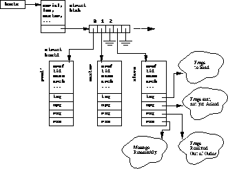
Figure: Host table
Host tables are issued by the master pvmd
and kept synchronized across the virtual machine.
The delete operation is simple:
On receiving a
DM_HTDEL message from the master,
a pvmd calls
hostfailentry()
for each host listed in the message,
as though the deleted pvmds crashed.
Each pvmd can autonomously delete hosts
from its own table on finding them
unreachable (by timing out during communication).
The add operation is done
with a three-phase commit,
in order to guarantee global availability of new hosts
synchronously with completion of the add-host request.
This is described in
Section
.
Each host descriptor has a refcount
so it can be
shared by multiple host tables.
As the configuration of the machine changes,
the host descriptors (except those added and deleted, of course)
propagate from one host table to the next.
This propagation is necessary because they hold various state information.
Host tables also serve other uses:
They allow the pvmd to manipulate host sets,
for example, when picking candidate hosts on which to spawn a task.
Also,
the advisory host file supplied to the master pvmd is
parsed and stored in a host table.
Host File
Next:
Tasks
Up:
Host Table and
Previous:
Host Table and
If the master pvmd is started with a host file,
it parses the file into a host table, filehosts.
If some hosts in the file are to be started automatically,
the master
sends a
DM_ADD message to itself.
The slave hosts are started
just as though they had been added dynamically
(Section
).
Introduction
Next:
Heterogeneous Network Computing
Up:
PVM: Parallel Virtual Machine
Previous:
Acknowledgments
Parallel processing,
the method of having many small tasks solve one large problem,
has emerged as a key enabling technology in modern computing.
The past several years have witnessed an ever-increasing acceptance
and adoption of parallel processing, both for high-performance
scientific computing and for more ``general-purpose'' applications,
was a result of the demand for
higher performance, lower cost, and sustained productivity.
The acceptance has been facilitated by two
major developments: massively parallel processors
(MPPs)
and the widespread use of distributed computing.
MPPs are now
the most powerful computers in the world.
These machines combine a few hundred to a few thousand CPUs
in a single large cabinet connected to hundreds of gigabytes of memory.
MPPs offer enormous computational power and are used to
solve computational Grand Challenge problems
such as global climate modeling and drug design.
As simulations become more realistic, the computational power
required to produce them grows rapidly.
Thus, researchers on the cutting edge
turn to MPPs and parallel processing
in order to get the most computational power possible.
The second major development affecting scientific problem solving is
distributed computing
.
Distributed computing is a process whereby a set of
computers connected by a network are used collectively
to solve a single large problem.
As more and more organizations have high-speed local area networks
interconnecting many general-purpose workstations,
the combined computational resources
may exceed the power of a single high-performance computer.
In some cases, several MPPs have been combined
using distributed computing to produce unequaled computational power.
The most important factor in distributed computing is cost.
Large MPPs typically cost more than $10 million.
In contrast,
users see very little cost in running their problems
on a local set of existing computers.
It is uncommon for distributed-computing users to realize
the raw computational power of a large MPP, but they are
able to solve problems several times larger than they could
using one of their local computers.
Common between distributed computing and MPP is the notion
of message passing
. In all parallel processing, data must
be exchanged between cooperating tasks.
Several paradigms have been tried including
shared memory, parallelizing compilers, and message passing.
The message-passing model has become
the paradigm of choice, from the
perspective of the number and variety of multiprocessors that support it,
as well as in terms of applications,
languages, and software systems that use it.
The Parallel Virtual Machine (PVM) system described in this book uses the message-passing
model to allow programmers to exploit distributed computing
across a wide variety of computer types, including MPPs.
A key concept in PVM is that it makes a collection of computers
appear as one large virtual machine
,
hence its name.
Next:
Heterogeneous Network Computing
Up:
PVM: Parallel Virtual Machine
Previous:
Acknowledgments
Tasks
Next:
Wait Contexts
Up:
PVM Daemon
Previous:
Host File
Each pvmd
maintains a list of all tasks under its management
(Figure
).
Every task, regardless of state, is a member of a
threaded list,
sorted by task id.
Most tasks are also in a second list,
sorted by process id.
The head of both lists is
locltasks.
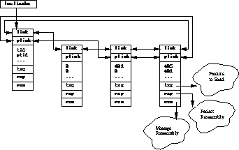
Figure: Task table
PVM provides a simple debugging system
described in Section
.
More complex debuggers can be built by using
a special type of task called a tasker, introduced in version 3.3.
A tasker starts (execs, and is the parent of)
other tasks.
In general,
a debugger is a process that
controls the execution of other processes - can read and write
their memories and start and stop instruction counters.
On many species of Unix,
a debugger must be the direct parent of any processes it controls.
This is becoming less common with growing availability of the
attachable ptrace interface.
The function of the tasker interface overlaps with the simple
debugger starter,
but is fundamentally different for two reasons:
First,
all tasks running under a pvmd (during the life of the tasker)
may be children of a single tasker process.
With PvmTaskDebug,
a new debugger is necessarily started for each task.
Second,
the tasker cannot be enabled or disabled by spawn flags,
so it is always in control,
though
this is not an important difference.
If a tasker is registered (using pvm_reg_tasker())
with a pvmd when a DM_EXEC
message is received to start new tasks,
the pvmd sends a SM_STTASK message to the tasker instead
of calling execv().
No SM_STTASKACK message is required;
closure comes from the task reconnecting to the pvmd as usual.
The pvmd doesn't get SIGCHLD signals when a tasker
is in use,
because it's not the parent process of tasks,
so the tasker must send notification of exited tasks
to the pvmd in a SM_TASKX message.
Next:
Wait Contexts
Up:
PVM Daemon
Previous:
Host File
Wait Contexts<A NAME=1123>
</A>
Next:
Fault Detection and
Up:
PVM Daemon
Previous:
Tasks
The pvmd uses a wait context (waitc) to hold state when
a thread of operation must be interrupted.
The pvmd is not truly multithreaded
but performs operations concurrently.
For example,
when a pvmd gets a syscall from a task
and
must interact with another pvmd,
it doesn't block while waiting for the other pvmd
to respond.
It
saves state in a
waitc
and returns immediately to the work() loop.
When the reply arrives,
the pvmd uses the information stashed
in the waitc
to complete the syscall and reply to the task.
Waitcs are serial numbered, and the number is sent in the
message header along with the request and
returned with the reply.
For many operations,
the TIDs and kind of wait are the
only information saved.
The struct waitc includes a few extra fields
to handle most of the remaining cases,
and a pointer,
wa_spec,
to a block of extra data for special cases-the
spawn and host startup operations,
which need to save
struct waitc_spawn and struct waitc_add.
Sometimes
more than one phase of waiting is necessary-in
series, parallel,
or nested.
In the parallel case, a separate waitc is created for each foreign host.
The waitcs are
peered (linked in a list)
together to indicate they pertain to the same operation.
If a waitc has no peers,
its peer links point to itself.
Usually,
peered waitcs share data,
for example, wa_spec.
All existing parallel operations
are conjunctions;
a peer group is finished when every waitc
in the group is finished.
As replies arrive,
finished waitcs are collapsed out of the list and deleted.
When the
finished waitc is the only one left,
the operation is complete.
Figure
shows single and peered waitcs
stored in
waitlist (the list
of all active waitcs).
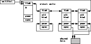
Figure: Wait context list
When a host fails or a task exits,
the pvmd
searches waitlist
for any blocked on this TID
and terminates those operations.
Waitcs from the dead host or task blocked on something else
are not deleted;
instead, their wa_tid fields are zeroed.
This approach prevents the wait id's from being recycled while
replies are still pending.
Once the defunct waitcs are satisfied,
they are silently discarded.
Next:
Fault Detection and
Up:
PVM Daemon
Previous:
Tasks
Fault Detection and Recovery
Next:
Pvmd'
Up:
PVM Daemon
Previous:
Wait Contexts
Fault detection
originates in the pvmd-pvmd
protocol
(Section
).
When the pvmd times out while communicating with another,
it calls hostfailentry(),
which scans waitlist and terminates any operations waiting
on the down host.
A pvmd can recover from the loss of any foreign pvmd
except the master.
If a slave loses the master,
the slave shuts itself down.
This algorithm ensures that the virtual machine doesn't become partitioned
and run as two partial machines.
It does, however, decrease fault tolerance
of the virtual machine
because the master must never crash.
There is currently no way for the master to hand off its status
to another pvmd,
so it always remains part of the configuration.
(This is an improvement over
PVM 2,
in which the failure of any pvmd would shut down the entire system.)
Pvmd'
Next:
Starting Slave Pvmds
Up:
PVM Daemon
Previous:
Fault Detection and
The shadow pvmd
(pvmd') runs on the master host
and is used by the master to start new slave pvmds.
Any of several steps in the startup process (for example,
starting a shell on the remote machine)
can block for seconds or minutes (or hang),
and the master pvmd must be able to
respond to other messages during this time.
It's messy to save all the state involved,
so a completely separate process is used.
The pvmd' has host number 0
and communicates with the master through the
normal pvmd-pvmd interface,
though
it never talks to tasks or other pvmds.
The normal host failure detection mechanism is used to
recover
in the event the pvmd' fails.
The startup operation has a wait context
in the master pvmd.
If the pvmd' breaks,
the master catches a SIGCHLD from it and
calls hostfailentry(),
which cleans up.
Starting Slave Pvmds
Next:
Resource Manager
Up:
PVM Daemon
Previous:
Pvmd'
Getting a slave pvmd
started is a messy task
with no good solution.
The goal is to
get a process running on the new host,
with enough
identity
to let it be fully configured and added
as a peer.
Ideally,
the mechanism used
should be
widely available, secure, and fast,
while
leaving the system easy to install.
We'd like to avoid having to type passwords all the time,
but don't want to put them in a file from where they can be stolen.
No one system meets all of these criteria.
Using
inetd
or
connecting to an already-running pvmd or pvmd server at a
reserved port
would allow fast,
reliable startup,
but would require that a system
administrator install PVM on each host.
Starting the pvmd
via
rlogin
or telnet
with a chat
script
would allow access even to
IP-connected hosts behind firewall machines
and
would require no special privilege
to install;
the main drawbacks are speed
and the
effort needed to get the chat program working
reliably.
Two widely available systems are
rsh
and rexec()
;
we
use both to cover the cases where a password
does and does not
need to be typed.
A manual startup
option allows the user to take the place of a
chat program,
starting the pvmd by hand and typing in the configuration.
rsh is a privileged program that can be
used to run commands on another host without a password,
provided the destination host
can be made to trust the source host.
This can be done either
by making it equivalent (requires a system administrator)
or by creating a .rhosts file on the destination host
(this isn't a great idea).
The alternative,
rexec(), is a function compiled into the pvmd.
Unlike rsh,
which doesn't take a password,
rexec() requires the user to supply one at run time,
either by typing it in
or by placing it in a .netrc file (this is a really bad idea).
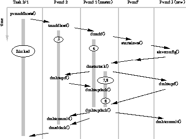
Figure: Timeline of addhost operation
Figure
shows
a host being added to the machine.
A task calls pvm_addhosts()
to
send a request to its pvmd,
which in turn sends a DM_ADD message to the master
(possibly itself).
The master pvmd
creates a new host table entry for each
host
requested,
looks up the IP addresses,
and sets the options
from host file entries
or defaults.
The host descriptors are kept in a waitc_add structure
(attached to a wait context)
and not yet added to the host table.
The master
forks the pvmd'
to do the dirty work,
passing it a list of hosts and commands to execute
(an SM_STHOST message).
The pvmd' uses rsh, rexec() or manual startup
to start each pvmd,
pass it parameters,
and
get a line of configuration data back.
The configuration dialog between pvmd'
and a new slave is as follows:
---------------------------------------------------------------------------
pvmd' --> slave: (exec) $PVM_ROOT/lib/pvmd -s -d8 -nhonk 1 80 a9ca95:0f5a
4096 3 80a95c43:0000
slave --> pvmd': ddpro<2312> arch
ip<80a95c43:0b3f> mtu<4096>
pvmd' --> slave: EOF
---------------------------------------------------------------------------
The
addresses of the master and slave pvmds
are passed on the command line.
The slave writes its configuration on standard output,
then waits for
an EOF from the pvmd'
and disconnects.
It runs in
probationary status
(runstate = PVMDSTARTUP)
until it
receives the rest of its configuration
from the master pvmd.
If it isn't configured within five minutes
(parameter DDBAILTIME),
it assumes there is some problem with the master
and quits.
The protocol revision
(DDPROTOCOL)
of the slave pvmd must match that of the master.
This number is incremented whenever a change in the protocol
makes it incompatible with the previous
version.
When several hosts are added at once,
startup is done in parallel.
The pvmd' sends the data (or errors)
in a DM_STARTACK message
to the
master pvmd,
which completes the host descriptors
held in the wait context.
If a special task
called a hoster
is registered with the master pvmd when it receives
the DM_ADD message,
the pvmd' is not used.
Instead,
the SM_STHOST message
is sent to the hoster,
which
starts the remote processes as described above
using any mechanism it wants,
then
sends a SM_STHOSTACK message (same format as DM_STARTACK)
back to the master pvmd.
Thus,
the method of starting slave pvmds is dynamically replaceable,
but the hoster does not have to understand the configuration
protocol.
If the hoster task fails during an add operation,
the pvmd uses the wait context to recover.
It assumes none of the slaves were started
and sends a DM_ADDACK message indicating a system error.
After the slaves are started,
the master
sends each a DM_SLCONF message
to set parameters not included in the startup protocol.
It then
broadcasts a DM_HTUPD message
to all new and existing slaves.
Upon receiving this message,
each slave knows the configuration of
the new virtual machine.
The master waits for an acknowledging DM_HTUPDACK message
from every slave,
then broadcasts
an HT_COMMIT message,
shifting all to the new host table.
Two phases are needed so that new hosts are not advertised
(e.g., by pvm_config()) until all pvmds know the new
configuration.
Finally,
the master
sends a DM_ADDACK reply to the original request,
giving the new host id's.
Note:
Recent experience suggests it would be cleaner to
manage the pvmd' through
the task interface
instead of the host interface.
This approach would allow
multiple starters to run at once
(parallel startup is implemented explicitly
in a single pvmd' process).
Next:
Resource Manager
Up:
PVM Daemon
Previous:
Pvmd'
Resource Manager<A NAME=1215>
</A>
Next:
Libpvm Library
Up:
PVM Daemon
Previous:
Starting Slave Pvmds
A resource manager (RM) is a PVM task
responsible for making task and host
scheduling (placement) decisions.
The resource manager interface was introduced in version 3.3.
The simple schedulers embedded in the pvmd
handle many common conditions,
but require the user to explicitly place program components in
order to get the maximum efficiency.
Using knowledge not available to the pvmds, such as host load averages,
a RM can make more informed decisions automatically.
For example, when spawning a task,
it could pick the host in order to balance the computing load.
Or, when reconfiguring the virtual machine,
the RM could interact with an external queuing
system to allocate a new host.
The number of RMs registered can vary
from one for an entire virtual machine to one per pvmd.
The RM running on the master host (where the master pvmd runs)
manages any slave pvmds that don't have their own RMs.
A task connecting anonymously to a virtual machine is assigned
the default RM of the pvmd to which it connects.
A task spawned from within the system inherits the RM
of its parent task.
If a task has a RM assigned to it,
service requests from the task to its pvmd are routed to the
RM instead.
Messages from the following libpvm functions are intercepted:
------------------------------------------------
Libpvm function Default Message RM Message
------------------------------------------------
pvm_addhost() TM_ADDHOST SM_ADDHOST
pvm_delhost() TM_DELHOST SM_DELHOST
pvm_spawn() TM_SPAWN SM_SPAWN
------------------------------------------------
Queries also go to the RM,
since it presumably knows more about the state of the virtual machine:
------------------------------------------------
Libpvm function Default Message RM Message
------------------------------------------------
pvm_config() TM_CONFIG SM_CONFIG
pvm_notify() TM_NOTIFY SM_NOTIFY
pvm_task() TM_TASK SM_TASK
------------------------------------------------
The call to register a task as a RM (pvm_reg_rm())
is also redirected if RM is already running.
In this way the existing RM learns of the new one,
and can grant or refuse the request to register.
Using messages SM_EXEC and SM_ADD,
the RM can directly command the pvmds to start tasks or reconfigure
the virtual machine.
On receiving acknowledgement for the commands,
it replies to the client task.
The RM is free to interpret service request parameters
in any way it wishes.
For example,
the architecture class given to pvm_spawn()
could be used to distinguish hosts by memory size or CPU speed.
Next:
Libpvm Library
Up:
PVM Daemon
Previous:
Starting Slave Pvmds
Libpvm Library
Next:
Language Support
Up:
How PVM Works
Previous:
Resource Manager
Language Support
Next:
Connecting to the
Up:
Libpvm Library
Previous:
Libpvm Library
Libpvm is
written in C and
directly supports C and C++ applications.
The Fortran
library,
libfpvm3.a
(also written in C),
is a set of wrapper functions
that conform to the Fortran calling conventions.
The Fortran/C linking requirements are portably met by preprocessing the
C source code for the
Fortran library with m4
before compilation.
Connecting to the Pvmd<A NAME=1247>
</A>
Next:
Protocols
Up:
Libpvm Library
Previous:
Language Support
On the first call to a libpvm function,
pvm_beatask() is called to
initialize the library state and
connect the task to its pvmd.
Connecting (for anonymous tasks)
is slightly different
from
reconnecting (for spawned tasks).
The pvmd publishes the address of the socket on which it listens
in /tmp/pvmd.uid,
where uid is the numeric user id under which the pvmd runs.
This file contains a line of the form
7f000001:06f7 or /tmp/aaa014138
This is the IP address and port number (in hexadecimal) of the socket,
or the path if a Unix-domain socket.
To avoid the need to read the address file,
the same information is passed to spawned tasks in
environment variable PVMSOCK.
To reconnect,
a spawned task also needs
its expected process id.
When a task is spawned by the pvmd,
a task descriptor
is created for it during the exec phase.
The descriptor must
exist
so it can stash any messages that arrive for the task
before it reconnects and can receive them.
During reconnection,
the task identifies itself to the pvmd by its PID.
If the task is always the child of the pvmd
(i.e., the exact process exec'd by it),
then it could use the value returned by getpid().
To allow for intervening processes,
such as debuggers,
the pvmd passes the expected PID in environment variable
PVMEPID,
and the task
uses that value in preference to its real PID.
The task also passes its real PID so it can be controlled normally
by the pvmd.
pvm_beatask() creates a TCP socket and does a proper connection
dance with the pvmd.
Each must prove its identity to the other,
to prevent a different user from spoofing the system.
It does this by creating a file in /tmp writable only by the owner,
and challenging the other to write in the file.
If successful,
the
identity of the other is proven.
Note that this authentication is only as strong as the filesystem
and the authority of root on each machine.
A protocol serial number
(TDPROTOCOL)
is compared whenever a task connects to a pvmd or another task.
This number is incremented whenever a change in the protocol
makes it incompatible with the previous
version.
Disconnecting is much simpler.
It can be done forcibly by a close from either end,
for example, by exiting the task process.
The function pvm_exit() performs a clean shutdown,
such that the process can be connected again later
(it would get a different TID).
Next:
Protocols
Up:
Libpvm Library
Previous:
Language Support
Protocols<A NAME=1267>
</A>
Next:
Messages
Up:
How PVM Works
Previous:
Connecting to the
PVM communication is based on TCP
,
UDP
,
and Unix-domain sockets.
While more appropriate
protocols exist,
they aren't as generally available.
VMTP
[3]
is one example of a protocol built for this purpose.
Although intended for RPC-style interaction
(request-response),
it could support PVM messages.
It is packet oriented
and efficiently sends short blocks
of data (such as most pvmd-pvmd management messages)
but also handles streaming (necessary for task-task communication).
It supports multicasting
and priority data (something PVM doesn't need yet).
Connections don't need to be established before use;
the first communication initializes the protocol drivers
at each end.
VMTP was rejected, however.
because
it is not widely available
(using it requires modifying the kernel).
This section explains the PVM protocols.
There are three connections to consider:
Between pvmds,
between pvmd and task,
and between tasks.
Heterogeneous Network Computing
Next:
Trends in Distributed
Up:
Introduction
Previous:
Introduction
In an MPP, every processor is exactly like every other
in capability, resources, software, and communication speed.
Not so on a network.
The computers available on a network
may be
made by different vendors or have different compilers.
Indeed, when a programmer wishes to exploit a
collection of networked computers, he may have to contend
with several different types of heterogeneity
:
- architecture,
- data format,
- computational speed,
- machine load,
and
- network load.
The set of computers available can include a wide range of architecture types
such as 386/486 PC class machines, high-performance workstations,
shared-memory multiprocessors, vector supercomputers, and even
large MPPs. Each architecture type has its own optimal programming method.
In addition, a user can be faced with a hierarchy of programming
decisions. The parallel virtual machine may itself be composed
of parallel computers.
Even when the architectures are only serial workstations,
there is still the problem of incompatible binary formats
and the need to compile a parallel task on each different
machine.
Data formats on different computers are often incompatible.
This incompatibility is an important point in distributed computing because
data sent from one computer may be unreadable on the receiving computer.
Message-passing packages developed for heterogeneous environments
must make sure all the computers understand the exchanged data.
Unfortunately,
the early message-passing systems developed for specific MPPs
are not amenable to distributed computing because they
do not include enough information in the message to
encode or decode it for any other computer.
Even if the set of computers are all workstations with the same data format,
there is still heterogeneity due to different computational speeds.
As an simple example, consider the problem of running
parallel tasks on a virtual machine that is composed of
one supercomputer and one workstation. The programmer must be careful
that the supercomputer doesn't sit idle waiting for the next data
from the workstation before continuing.
The problem of computational speeds can be very subtle.
The virtual machine can be composed of a set of identical workstations.
But since networked computers can have several other users on them
running a variety of jobs, the machine load can vary dramatically.
The result is that the effective computational power across
identical workstations can vary by an order of magnitude.
Like machine load, the time it takes to send a message over the network
can vary depending on the network load imposed by all the other network
users, who may not even be using any of the computers in the virtual
machine. This sending time becomes important when a task is sitting
idle waiting for a message, and it is even more important when
the parallel algorithm is sensitive to message arrival time.
Thus, in distributed computing, heterogeneity can appear dynamically
in even simple setups.
Despite these numerous difficulties caused by heterogeneity,
distributed computing offers
many advantages:
-
By using existing hardware, the cost of this computing can be very low.
-
Performance can be optimized by assigning each individual task
to the most appropriate architecture.
-
One can exploit the heterogeneous nature of a computation.
Heterogeneous network computing is not just a local area network
connecting workstations together.
For example, it provides access to different data bases or to special
processors for those parts of an application that can run only on a certain
platform.
-
The virtual computer resources can grow in stages and take
advantage of the latest computational and network technologies.
-
Program development can be enhanced by using a familiar environment.
Programmers can use editors, compilers, and debuggers
that are available on individual machines.
-
The individual computers and workstations are usually stable, and substantial
expertise in their use is readily available.
-
User-level or program-level fault tolerance can be implemented with
little effort either in the application or in the underlying
operating system.
-
Distributed computing can facilitate collaborative work.
All these factors translate into reduced development and debugging time,
reduced contention for resources, reduced costs, and possibly more
effective implementations of an application.
It is these benefits that PVM seeks to exploit.
From the beginning,
the PVM software package
was designed to make programming for a
heterogeneous collection of machines straightforward.
Next:
Trends in Distributed
Up:
Introduction
Previous:
Introduction
Messages
Next:
Pvmd-Pvmd
Up:
Protocols
Previous:
Protocols
The pvmd and libpvm use the same message header,
shown in Figure
.
Code
contains an integer tag (message type).
Libpvm uses
Encoding
to pass the encoding
style of the message, as it can pack in different
formats.
The pvmd always sets Encoding (and requires that it be set)
to 1 (foo),
Pvmds use
the
Wait Context
field
to pass the wait id's (if any, zero if none)
of the waitc
associated with the message.
Certain tasks (resource manager, tasker, hoster)
also use wait id's.
The
Checksum
field is reserved for future use.
Messages are sent in one or more fragments,
each with its own fragment header (described below).
The message header is at the beginning of the first fragment.
Figure: Message header
Pvmd-Pvmd<A NAME=1285>
</A>
Next:
Pvmd-Task and Task-Task
Up:
Protocols
Previous:
Messages
PVM daemons communicate with one another through UDP sockets.
UDP is an unreliable
delivery service which can lose,
duplicate or reorder packets,
so
an acknowledgment and retry mechanism is used.
UDP also limits packet length,
so
PVM fragments long messages.
We
considered TCP,
but three factors make it inappropriate.
First is scalability
.
In a virtual machine of N hosts,
each pvmd must have connections to the other N - 1.
Each open TCP connection consumes
a file descriptor in the pvmd,
and some operating systems limit the number of open files to as few as 32,
whereas
a single UDP socket can communicate with any number of remote
UDP sockets.
Second is overhead
.
N pvmds
need
N(N - 1)/2
TCP connections,
which would be expensive to set up.
The PVM/UDP protocol is initialized with no communication.
Third is fault tolerance
.
The communication system
detects when foreign pvmds
have crashed
or the network has gone down,
so
we need to set timeouts in the protocol layer.
The TCP keepalive option might work,
but
it's not always possible to get
adequate control over the
parameters.
The packet header
is shown in Figure
.
Multibyte values are sent in (Internet) network byte order
(most significant byte first).
Figure: Pvmd-pvmd packet header
The source and destination fields hold
the TIDs of the true source and final destination of the packet,
regardless of the route it takes.
Sequence and acknowledgment numbers start at 1 and increment to 65535,
then wrap to zero.
SOM (EOM) - Set for the first (last) fragment of a message.
Intervening fragments have both bits cleared.
They are used by tasks and pvmds to delimit message boundaries.
DAT - If set, data is contained in the packet, and the sequence
number is valid.
The packet, even if zero length, must be delivered.
ACK - If set, the acknowledgment number field is valid.
This bit may be combined with the DAT bit to piggyback an acknowledgment
on a data packet.
FIN - The pvmd is closing down the connection.
A packet with FIN bit set (and DAT cleared)
begins an orderly shutdown.
When an acknowledgement arrives (ACK bit set and ack number
matching the sequence number from the FIN packet),
a final packet is sent with both FIN and ACK set.
If the pvmd panics,
(for example on a trapped segment violation)
it tries to send a packet with FIN and ACK set to
every peer before it exits.
The state of a connection to another pvmd is kept in its host table
entry.
The protocol driver uses the following fields of
struct hostd:
Field Meaning
-----------------------------------------------------
hd_hostpart TID of pvmd
hd_mtu Max UDP packet length to host
hd_sad IP address and UDP port number
hd_rxseq Expected next packet number from host
hd_txseq Next packet number to send to host
hd_txq Queue of packets to send
hd_opq Queue of packets sent, awaiting ack
hd_nop Number of packets in hd_opq
hd_rxq List of out-of-order received packets
hd_rxm Buffer for message reassembly
hd_rtt Estimated smoothed round-trip time
-----------------------------------------------------
Figure
shows
the host send and outstanding-packet queues.
Packets waiting to be sent to a host are queued in FIFO
hd_txq.
Packets
are appended to this queue by the routing code,
described in
Section
.
No receive queues are used;
incoming packets are passed immediately through
to other send queues or reassembled into messages (or discarded).
Incoming messages are delivered to a pvmd
entry point as described in
Section
.

Figure: Host descriptors with send queues
The protocol allows multiple outstanding packets
to improve performance over high-latency networks,
so two more queues are required.
hd_opq
holds a per-host list of unacknowledged packets,
and global opq
lists all unacknowledged packets,
ordered by time to retransmit.
hd_rxq holds packets received out of sequence until they
can be accepted.
The difference in time between sending a packet
and getting the acknowledgement is
used to estimate the round-trip time to the foreign host.
Each update is filtered into the estimate according to the formula
 .
.
When the acknowledgment for a packet arrives,
the packet
is removed from hd_opq and opq and discarded.
Each packet has a retry timer and count,
and each is resent until acknowledged by the foreign pvmd.
The timer starts at
3 * hd_rtt,
and doubles for each retry up to 18 seconds.
hd_rtt
is limited to nine seconds, and backoff is
bounded in order to allow at least 10 packets to be sent to a host
before giving up.
After three minutes of resending with no acknowledgment,
a packet expires.
If a packet expires as a result of timeout,
the foreign pvmd is assumed to be down or unreachable,
and the local pvmd gives up on it,
calling hostfailentry()
Next:
Pvmd-Task and Task-Task
Up:
Protocols
Previous:
Messages
Pvmd-Task <A NAME=1335>
</A> and Task-Task
<A NAME=1336>
</A>
Next:
Message Routing
Up:
Protocols
Previous:
Pvmd-Pvmd
A task talks to its pvmd and other tasks through TCP sockets.
TCP is used
because it delivers data reliably.
UDP can lose packets
even within a host.
Unreliable delivery requires retry
(with timers)
at both ends:
since tasks can't be
interrupted while computing to perform I/O,
we can't use UDP.
Implementing a
packet service over TCP is
simple
because of its reliable delivery.
The packet header is shown in
Figure
.
No sequence numbers are needed,
and only flags SOM and EOM
(these have the same meaning as in Section
).
Since TCP
provides no record marks to
distinguish back-to-back packets from one another,
the length is sent in the header.
Each side maintains a
FIFO of packets to send,
and switches between reading
the socket when data is available
and writing when there is space.
Figure: Pvmd-task packet header
The main drawback to TCP (as opposed to UDP)
is that more system
calls are needed to transfer each packet.
With UDP,
a single
sendto()
and
single
recvfrom()
are required.
With TCP,
a packet can be sent by a single
write() call,
but
must be received by two
read() calls,
the first to get the header and the second to get the data.
When traffic on the connection is heavy,
a simple optimization reduces the average number of reads back
to about one per packet.
If,
when reading the packet body,
the requested length is increased by the size of a
packet header,
the read may succeed in getting both the packet body
and header of the next packet at once.
We have the header for the next packet for free
and can repeat this process.
Version 3.3 introduced the use of Unix-domain stream sockets as an
alternative to TCP for local communication,
to improve latency and transfer rate
(typically by a factor of two).
If enabled (the system is built without the NOUNIXDOM
option),
stream sockets are used between the pvmd and tasks
as well as between tasks on the same host.
Next:
Message Routing
Up:
Protocols
Previous:
Pvmd-Pvmd
Message Routing<A NAME=1353>
</A>
Next:
Pvmd
Up:
How PVM Works
Previous:
Pvmd-Task and Task-Task
Pvmd
Next:
Packet Buffers
Up:
Message Routing
Previous:
Message Routing
Packet Buffers<A NAME=1356>
</A>
Next:
Message Routing
Up:
Pvmd
Previous:
Pvmd
Packet descriptors (struct pkt)
track message fragments
through
the pvmd.
Fields
pk_buf, pk_max, pk_dat and pk_len
are used in the same ways as
similarly named fields of a frag,
described in
Section
.
Besides data,
pkts contain state to operate
the pvmd-pvmd protocol.
Message Routing<A NAME=1363>
</A>
Next:
Packet Routing
Up:
Pvmd
Previous:
Packet Buffers
Messages are sent by calling sendmessage(),
which routes by destination address.
Messages for other pvmds or tasks
are linked to packet descriptors and attached
to a send queue.
If the pvmd addresses a message to itself,
sendmessage()
passes the whole message descriptor
to netentry(),
avoiding the packet layer entirely.
This loopback interface is used often by the pvmd.
During a complex operation,
netentry() may be reentered several times
as the pvmd sends itself messages.
Messages to the pvmd are reassembled from packets
in message reassembly buffers,
one for each local task and remote pvmd.
Completed messages are passed to entry points (Section
).
Packet Routing<A NAME=1369>
</A>
Next:
Refragmentation
Up:
Pvmd
Previous:
Message Routing
A graph of packet and message routing inside the pvmd is shown in
Figure
.
Packets are received from the network
by
netinput()
directly into buffers
long enough to hold the largest packet
the pvmd will receive (its MTU in the host table).
Packets from local tasks
are read by loclinput(),
which creates a buffer large enough for each packet
after it reads the header.
To route a packet,
the pvmd chains it onto
the queue for its destination.
If a packet is multicast
(see Section
),
the descriptor is replicated,
counting extra
references on the underlying databuf.
One copy is placed in each send queue.
After the last copy of the packet is sent,
the databuf is freed.
Figure: Packet and message routing in pvmd
Refragmentation<A NAME=1379>
</A>
Next:
Pvmd and Foreign
Up:
Pvmd
Previous:
Packet Routing
Messages are generally built
with fragment length
equal to the MTU of the host's pvmd,
allowing them to be forwarded without refragmentation.
In some cases,
the pvmd can receive a packet (from a task) too long
to be sent to another pvmd.
The pvmd refragments
the packet by replicating its descriptor
as many times as necessary.
A single databuf is shared between the descriptors.
The pk_dat and pk_len fields of the
descriptors
cover successive chunks of the original
packet,
each chunk small enough to send.
The SOM and EOM flags are adjusted
(if the original packet is the start or end of a message).
At send time, netoutput()
saves the data under where it
writes the packet header,
sends the packet,
and
then restores the data.
PVM: Parallel Virtual Machine: A Users' Guide and Tutorial for Networked Parallel Computing
PVM: Parallel Virtual Machine
A Users' Guide and Tutorial for
Networked Parallel Computing
pvm@msr.epm.ornl.gov

Next:
Contents
MIT Press
Scientific and Engineering ComputationJanusz Kowalik, Editor
 1994 Massachusetts Institute of Technology
All rights reserved. No part of this book may be reproduced
in any form by any electronic or mechanical means (including
photocopying, recording, or information storage and retrieval)
without permission in writing from the publisher.
This book was set in  by the authors and was
printed and bound in the United States of America.
by the authors and was
printed and bound in the United States of America.
Library of Congress Cataloging-in-Publication Data
This book is also available in postscript and html forms over the Internet.
To retrieve the postscript file you can use one of the following methods:
- anonymous ftp
- ftp ftp.netlib.org
- cd pvm3/book
- get pvm-book.ps
- quit
-
from any machine on the Internet type:
- rcp anon@anonrcp.netlib.org:pvm3/book/pvm-book.ps pvm-book.ps
- sending email to
netlib@netlib.org and in the message type:
send pvm-book.ps from pvm3/book
- use Xnetlib and click ``library", click ``pvm3", click ``book",
click ``pvm3/pvm-book.ps", click ``download", click ``Get Files Now".
(Xnetlib is an X-window interface to the netlib software
based on a client-server model. The software can
be found in netlib, ``send index from xnetlib'').
To view the html file use the URL:
-
http://www.netlib.org/pvm3/book/pvm-book.html
To order from the publisher, send email to mitpress-orders@mit.edu,
or telephone 800-356-0343 or 617-625-8569. Send snail mail orders to
- The MIT Press
- Book Order Department
- 55 Hayward Street
- Cambridge, MA 02142.
8 x 9 * 176 pages * $17.95 * Original in Paperback ISBN 0-262-57108-0
For more information, contact Gita Manaktala, manak@mit.edu.
or
-
Click here
Thu Sep 15 21:00:17 EDT 1994
Next:
Contents
Jack Dongarra
Thu Sep 15 21:00:17 EDT 1994
Matrix Multiply<A NAME=881>
</A>
Next:
Example program: mmult.c
Up:
Program Examples
Previous:
Example program: failure.c
In our next example we program a matrix-multiply algorithm described by Fox
et al. in
[5]. The mmult program can be found at the end of this
section.
The mmult program will calculate  , where
 ,
, and
are all square matrices. For simplicity we
assume that
,
, and
are all square matrices. For simplicity we
assume that  tasks will be used to calculate the solution.
Each task will calculate a subblock of the resulting matrix
. The
block size and the value of
tasks will be used to calculate the solution.
Each task will calculate a subblock of the resulting matrix
. The
block size and the value of  is given as a command line argument to
the program. The matrices
and
are also stored as blocks distributed
over the
tasks. Before delving into the details of the program,
let us first describe the algorithm at a high level.
is given as a command line argument to
the program. The matrices
and
are also stored as blocks distributed
over the
tasks. Before delving into the details of the program,
let us first describe the algorithm at a high level.
Assume we have a grid of
tasks. Each task (
where
 ) initially contains blocks
,
, and
. In the first step of the algorithm the tasks on the diagonal
(
where
) initially contains blocks
,
, and
. In the first step of the algorithm the tasks on the diagonal
(
where  ) send their block
to all the other tasks
in row
) send their block
to all the other tasks
in row  . After the transmission of
, all tasks calculate
and add the result into
. In the next
step, the column blocks of
are rotated. That is,
sends
its block of
to
. (Task
sends its
block
to
.) The tasks now return to the first step;
is multicast to all other tasks in row
, and the
algorithm continues. After
iterations the
matrix contains
. After the transmission of
, all tasks calculate
and add the result into
. In the next
step, the column blocks of
are rotated. That is,
sends
its block of
to
. (Task
sends its
block
to
.) The tasks now return to the first step;
is multicast to all other tasks in row
, and the
algorithm continues. After
iterations the
matrix contains  , and the
matrix has been rotated back into place.
, and the
matrix has been rotated back into place.
Let's now go over the matrix multiply as it is programmed in PVM. In
PVM there is no restriction on which tasks may communicate with which
other tasks. However, for this program we would like to think of the
tasks as a two-dimensional conceptual torus. In order to enumerate the
tasks, each task joins the group mmult. Group ids are used to
map tasks to our torus. The first task to join a group is given the
group id of zero. In the mmult program, the task with group id zero
spawns the other tasks and sends the parameters for the matrix multiply
to those tasks. The parameters are
and  : the square root of
the number of blocks and the size of a block, respectively. After all the
tasks have been spawned and the parameters transmitted,
: the square root of
the number of blocks and the size of a block, respectively. After all the
tasks have been spawned and the parameters transmitted,
pvm_barrier() is called to make sure all the tasks have joined
the group. If the barrier is not performed, later
calls to pvm_gettid() might fail since a task may not have yet
joined the group.
After the barrier, we store the task ids for the other tasks in our
``row'' in the array myrow. This is done by calculating the
group ids for all the tasks in the row and asking PVM for the task
id for the corresponding group id. Next we allocate the blocks for the
matrices using malloc(). In an actual application program we would
expect that the matrices would already be allocated. Next the program
calculates the row and column of the block of
it will be computing.
This is based on the value of the group id. The group ids range from
 to
to  inclusive. Thus the integer division of
  will
give the task's row and
will
give the task's row and  will give the column, if we assume
a row major mapping of group ids to tasks. Using a similar mapping, we
calculate the group id of the task directly above and below
in the torus and store their task ids in up and down,
respectively.
will give the column, if we assume
a row major mapping of group ids to tasks. Using a similar mapping, we
calculate the group id of the task directly above and below
in the torus and store their task ids in up and down,
respectively.
Next the blocks are initialized by calling InitBlock(). This function
simply initializes
to random values,
to the identity matrix, and
to zeros. This will allow us to verify the computation at the end of the
program by checking that  .
.
Finally we enter the main loop to calculate the matrix multiply. First
the tasks on the diagonal multicast their block of A to the other tasks
in their row. Note that the array myrow actually contains the
task id of the task doing the multicast. Recall that pvm_mcast() will
send to all the tasks in the tasks array except the calling task. This
procedure works well in the case of mmult since we don't want to have to needlessly
handle the extra message coming into the multicasting task with an extra
pvm_recv(). Both the multicasting task and the tasks receiving the block
calculate the  for the diagonal block and the block of
residing in
the task.
for the diagonal block and the block of
residing in
the task.
After the subblocks have been multiplied and added into the
block, we
now shift the
blocks vertically. Specifically, we pack the block
of
into a message, send it to the up task id, and then
receive a new
block from the down task id.
Note that we use different message tags for sending the
blocks and the
blocks as well as for different iterations of the loop. We also fully
specify the task ids when doing a pvm_recv(). It's tempting to use
wildcards for the fields of pvm_recv(); however, such a practice can be dangerous. For instance,
had we incorrectly calculated the value for up and used a wildcard
for the pvm_recv() instead of down,
we might have sent
messages to the wrong tasks without knowing it. In this example we fully
specify messages, thereby reducing the possibility of mistakes by receiving
a message from the wrong task or the wrong phase of the algorithm.
Once the computation is complete, we check to see that
, just to verify
that the matrix multiply correctly calculated the values of
. This check would
not be done in a matrix multiply library routine, for example.
It is not necessary to call pvm_lvgroup(), since PVM will
realize the task has exited and will remove it from the group. It is good
form, however, to leave the group before calling pvm_exit(). The
reset command from the PVM console will reset all the PVM groups. The
pvm_gstat command will print the status of any groups that
currently exist.
Next:
Example program: mmult.c
Up:
Program Examples
Previous:
Example program: failure.c
Pvmd and Foreign Tasks<A NAME=1385>
</A>
Next:
Libpvm
Up:
Message Routing
Previous:
Refragmentation
Pvmds usually don't communicate with foreign tasks
(those on other hosts).
The pvmd has message reassembly buffers for each foreign pvmd
and each task it manages.
What it doesn't want is to have reassembly buffers
for foreign tasks.
To free up the reassembly buffer for a foreign task
(if the task dies),
the pvmd
would have to request notification from the task's pvmd,
causing extra communication.
For the sake of simplicity
the pvmd local to the sending task serves as a message
repeater.
The message is reassembled
by the task's local pvmd as if it were the receiver,
then forwarded all at once to the
destination pvmd,
which reassembles the message again.
The source address is preserved,
so the sender can be identified.
Libpvm maintains dynamic reassembly buffers,
so
messages from pvmd to task do not cause a problem.
Control Messages<A NAME=1054>
</A>
Next:
PVM Daemon
Up:
Messages
Previous:
Pvmd Entry Points
Control messages are sent to a task like regular messages,
but have tags in a reserved space
(between TC_FIRST and TC_LAST).
Normally,
when a task downloads a message,
it queues it for receipt by the program.
Control messages are instead passed
to
pvmmctl()
and then discarded.
Like the entry points in the pvmd,
pvmmctl() is an entry point in the task,
causing it to take some asynchronous action.
The main difference is that
control messages
can't be used to get the task's attention,
since it must be in mxfer(),
sending or receiving,
in order
to get them.
The following control message tags are defined.
The first three are used by the direct routing mechanism
(discussed in Section
).
TC_OUTPUT is used to implement
pvm_catchout() (Section
).
User-definable control messages may
be added in the future as a way of implementing
PVM signal handlers
.
Pvmd Entry Points
Next:
Control Messages
Up:
Messages
Previous:
Messages in the
Messages for the pvmd
are reassembled from packets in loclinpkt()
if from a local task,
or in netinpkt() if from another pvmd or foreign task.
Reassembled messages are passed to one of three
entry points:

If the message tag and contents are valid,
a new thread of action is started to handle the request.
Invalid messages are discarded.
Resource Manager<A NAME=1215>
</A>
Next:
Libpvm Library
Up:
PVM Daemon
Previous:
Starting Slave Pvmds
A resource manager (RM) is a PVM task
responsible for making task and host
scheduling (placement) decisions.
The resource manager interface was introduced in version 3.3.
The simple schedulers embedded in the pvmd
handle many common conditions,
but require the user to explicitly place program components in
order to get the maximum efficiency.
Using knowledge not available to the pvmds, such as host load averages,
a RM can make more informed decisions automatically.
For example, when spawning a task,
it could pick the host in order to balance the computing load.
Or, when reconfiguring the virtual machine,
the RM could interact with an external queuing
system to allocate a new host.
The number of RMs registered can vary
from one for an entire virtual machine to one per pvmd.
The RM running on the master host (where the master pvmd runs)
manages any slave pvmds that don't have their own RMs.
A task connecting anonymously to a virtual machine is assigned
the default RM of the pvmd to which it connects.
A task spawned from within the system inherits the RM
of its parent task.
If a task has a RM assigned to it,
service requests from the task to its pvmd are routed to the
RM instead.
Messages from the following libpvm functions are intercepted:
Queries also go to the RM,
since it presumably knows more about the state of the virtual machine:
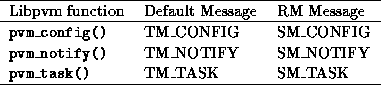
The call to register a task as a RM (pvm_reg_rm())
is also redirected if RM is already running.
In this way the existing RM learns of the new one,
and can grant or refuse the request to register.
Using messages SM_EXEC and SM_ADD,
the RM can directly command the pvmds to start tasks or reconfigure
the virtual machine.
On receiving acknowledgement for the commands,
it replies to the client task.
The RM is free to interpret service request parameters
in any way it wishes.
For example,
the architecture class given to pvm_spawn()
could be used to distinguish hosts by memory size or CPU speed.
Next:
Libpvm Library
Up:
PVM Daemon
Previous:
Starting Slave Pvmds
Environment Variables<A NAME=1447>
</A>
Next:
Standard Input and
Up:
Task Environment
Previous:
Task Environment
Experience seems to indicate
that inherited
environment (Unix environ)
is useful to an application.
For example,
environment variables can be used to
distinguish a group of related tasks
or to set debugging variables.
PVM makes increasing use of environment,
and may eventually support it
even on machines where the concept
is not native.
For now,
it allows a task to export any part of environ
to tasks spawned by it.
Setting variable PVM_EXPORT to the names of other variables
causes them to be exported through spawn.
For example, setting
PVM_EXPORT=DISPLAY:SHELL
exports the variables DISPLAY and SHELL to
children tasks (and PVM_EXPORT too).
The following environment variables are used by PVM.
The user may set these:
The following variables are set by PVM and should not be modified:
Standard Input and Output<A NAME=1480>
</A>
Next:
Tracing
Up:
Task Environment
Previous:
Environment Variables
Each task spawned through PVM
has /dev/null opened for stdin.
From its parent,
it inherits a stdout sink,
which is a (TID, code) pair.
Output on stdout or stderr is
read by the pvmd through a pipe,
packed into PVM messages and
sent to the TID,
with message tag equal to the code.
If the output TID is set to zero
(the default for a task with no parent),
the messages go to the master pvmd,
where they are written on its error log.
Children spawned by a task inherit its stdout
sink.
Before the spawn,
the parent can use pvm_setopt() to
alter the output TID or code.
This doesn't
affect where the output of the parent task itself goes.
A task may set output TID to one of three settings:
the value inherited from its parent,
its own TID,
or zero.
It can set output code only if output TID is set to its own TID.
This means that output can't be assigned to an arbitrary task.
Four types of messages are sent to an stdout sink.
The message body formats for each type are as follows:
The first two items in the message body
are always the task id and output count,
which
allow the receiver to
distinguish between different tasks and the four message types.
For each task,
one message each
of types Spawn, Begin, and End is sent,
along with zero or more messages of class Output, (count > 0).
Classes Begin, Output and End will be received
in order,
as they originate from the same source (the pvmd of the
target task).
Class Spawn originates at the (possibly different) pvmd
of the parent task,
so it can be received in any order relative to
the others.
The output sink
is expected to understand the different types of messages
and use them to know when to stop
listening for output from a task (EOF) or group of tasks (global EOF).
The messages are designed so as to prevent race conditions
when a task spawns another task,
then immediately exits.
The
output sink might
get the End
message from the parent task
and decide the group is finished,
only to receive more output later from the child task.
According to these rules, the Spawn
message for the second task
must
arrive before
the End message from the first task.
The Begin message itself is necessary because the Spawn
message for a task may arrive after the End message
for the same task.
The state transitions of a task as observed by the receiver of
the output messages
are shown in
Figure
.
Figure: Output states of a task
The libpvm function pvm_catchout() uses this output collection
feature to put the output from children of a task into a file
(for example, its own stdout).
It sets output TID to its own task id,
and the output code to control message TC_OUTPUT.
Output from children and grandchildren tasks is collected by the
pvmds and sent to the task,
where it is received by pvmmctl() and printed by pvmclaimo().
Next:
Tracing
Up:
Task Environment
Previous:
Environment Variables
Footnotes
- ...\title
-
This work was supported in part by
DARPA and ARO under contract number DAAL03-91-C-0047,
the National Science Foundation Science and Technology Center Cooperative
Agreement No. CCR-8809615,
the Applied Mathematical Sciences subprogram of the Office of
Energy Research, U.S. Department of Energy, under Contract
DE-AC05-84OR21400,
and
the Stichting Nationale Computer Faciliteit (NCF) by Grant CRG 92.03.
- ...\author
- Los Alamos National Laboratory,
Los Alamos, NM 87544.
- ...\author
- Department of Computer Science, University of
Tennessee, Knoxville, TN 37996-1301.
- ...\author
- Applied Mathematics Department,
University of California, Los Angeles, CA 90024-1555.
- ...\author
- Computer Science Division and Mathematics
Department, University of California, Berkeley, CA 94720.
- ...\author
- Mathematical Sciences Section,
Oak Ridge National Laboratory, Oak Ridge, TN 37831-6367.
- ...\author
- National Institute of Standards and Technology,
Gaithersburg, MD, 20899
- ...\author
- Department of Mathematics, Utrecht University, Utrecht, the
Netherlands.
- ...
- For a discussion of BLAS as building
blocks, see
[144]
[71]
[70]
[69] and
LAPACK routines
[3]. Also, see
Appendix
.
- ...
- For a more detailed account of the early
history of CG methods, we refer the reader to Golub and
O'Leary
[108] and
Hestenes
[123].
- ...
- Under certain conditions, one can show
that the point Jacobi algorithm is optimal, or close to optimal, in
the sense of reducing the condition number, among all
preconditioners of diagonal form. This was shown by Forsythe and
Strauss for matrices with Property A
[99], and by van der
Sluis
[198] for general sparse matrices. For
extensions to block Jacobi preconditioners, see
Demmel
[66] and Elsner
[95].
- ...
- The SOR and Gauss-Seidel matrices are never used as preconditioners,
for a rather technical reason.
SOR-preconditioning with optimal
 maps the eigenvalues of the
coefficient matrix to a circle in the complex plane;
see Hageman and Young [.3]HaYo:applied. In this case no
polynomial acceleration is possible, i.e., the accelerating polynomial
reduces to the trivial polynomial
maps the eigenvalues of the
coefficient matrix to a circle in the complex plane;
see Hageman and Young [.3]HaYo:applied. In this case no
polynomial acceleration is possible, i.e., the accelerating polynomial
reduces to the trivial polynomial  , and the resulting
method is simply the stationary SOR method.
Recent research by Eiermann and Varga
[84] has shown
that polynomial
acceleration of SOR with suboptimal
will yield no improvement
over simple SOR with optimal
.
, and the resulting
method is simply the stationary SOR method.
Recent research by Eiermann and Varga
[84] has shown
that polynomial
acceleration of SOR with suboptimal
will yield no improvement
over simple SOR with optimal
.
- ...
- To be precise, if we make an incomplete factorization
 , we
refer to positions in
, we
refer to positions in  and
and  when we talk of positions in the
factorization. The matrix
when we talk of positions in the
factorization. The matrix  will have more nonzeros than
and
combined.
will have more nonzeros than
and
combined.
- ...
- The zero refers to the fact that only ``level zero'' fill is
permitted, that is, nonzero elements of the original matrix. Fill
levels are defined by calling an element of level
 if it is
caused by elements at least one of which is of level
if it is
caused by elements at least one of which is of level  .
The first fill level is that caused by the original matrix elements.
.
The first fill level is that caused by the original matrix elements.
- ...
- In graph theoretical terms,
 and
and  -
- coincide if the matrix graph contains no triangles.
- ...
- Writing
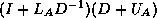 is equally valid, but in practice
harder to implement.
is equally valid, but in practice
harder to implement.
- ...
- On a machine with IEEE Standard
Floating Point Arithmetic,
 in single precision, and
  in double precision.
- ...
- IEEE standard
floating point arithmetic permits computations with
 and
NaN, or Not-a-Number, symbols.
and
NaN, or Not-a-Number, symbols.
- ...
Jack Dongarra
Mon Nov 20 08:52:54 EST 1995
How to Use This Book
Next:
Author's Affiliations
Up:
Templates for the Solution
Previous:
Templates for the Solution
We have divided this book into five main chapters.
Chapter
gives the motivation for this book
and the use of templates.
Chapter
describes
stationary and nonstationary iterative methods. In
this chapter we present both historical development and
state-of-the-art methods for solving some of the most challenging
computational problems facing researchers.
Chapter
focuses on preconditioners. Many
iterative methods depend in part on preconditioners to improve
performance and ensure fast convergence.
Chapter
provides a glimpse of issues related
to the use of iterative methods.
This chapter, like the preceding, is
especially recommended for the experienced user who wishes to have
further guidelines for tailoring a specific code to a particular
machine.
It includes information on complex systems, stopping criteria,
data storage formats, and parallelism.
Chapter
includes overviews of related
topics such as
the close connection between the Lanczos algorithm and the Conjugate
Gradient algorithm, block iterative methods,
red/black orderings,
domain decomposition methods,
multigrid-like methods, and
row-projection schemes.
The Appendices contain information on
how the templates and BLAS software can be
obtained.
A glossary of important terms used in the book is also provided.
The field of iterative methods for solving systems of linear equations
is in constant flux, with new methods and approaches continually being
created, modified, tuned, and some eventually discarded. We expect
the material in this book to undergo changes from time to time as some
of these new approaches mature and become the state-of-the-art.
Therefore, we plan to update the material included in this book
periodically for future editions. We welcome your comments and
criticisms of this work to help us in that updating process. Please
send your comments and questions by email to templates@cs.utk.edu.
List of Symbols
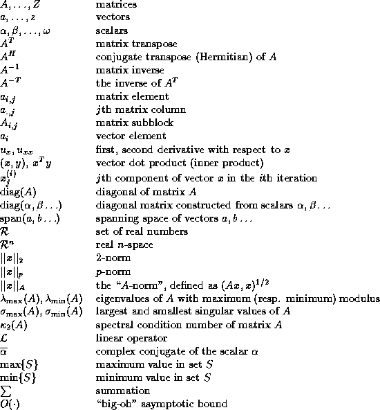
Jack Dongarra
Mon Nov 20 08:52:54 EST 1995
Overview of the Methods
Next:
Stationary Iterative Methods
Up:
Iterative Methods
Previous:
Iterative Methods
Below are short descriptions of each of the methods to be discussed,
along with brief notes on the classification of the methods in terms
of the class of matrices for which they are most appropriate. In
later sections of this chapter more detailed descriptions of these
methods are given.
- Stationary Methods
- Jacobi
.
The Jacobi method is based on solving for every variable locally with
respect to the other variables; one iteration of the method
corresponds to solving for every variable once. The resulting method
is easy to understand and implement, but convergence is slow.
- Gauss-Seidel
.
The Gauss-Seidel method is like the Jacobi method, except that it uses
updated values as soon as they are available.
In general, if the Jacobi method converges, the Gauss-Seidel method
will converge faster than the Jacobi method, though still relatively
slowly.
- SOR
.
Successive Overrelaxation (SOR) can be derived from the Gauss-Seidel
method by introducing an extrapolation parameter
. For the
optimal choice of
, SOR may converge faster than Gauss-Seidel by
an order of magnitude.
- SSOR
.
Symmetric Successive Overrelaxation (SSOR) has no advantage over SOR
as a stand-alone iterative method; however, it is useful as a
preconditioner for nonstationary methods.
- Nonstationary Methods
- Conjugate Gradient (CG
).
The conjugate gradient method derives its name from the fact that it
generates a sequence of conjugate (or orthogonal) vectors. These
vectors are the residuals of the iterates. They are also the
gradients of a quadratic functional, the minimization of which is
equivalent to solving the linear system. CG is an extremely effective
method when the coefficient matrix is symmetric positive definite,
since storage for only a limited number of vectors is required.
- Minimum Residual (MINRES
) and Symmetric LQ
(SYMMLQ
).
These methods are computational alternatives for CG for coefficient
matrices that are symmetric but possibly indefinite. SYMMLQ will
generate the same solution iterates as CG if the coefficient matrix is
symmetric positive definite.
- Conjugate Gradient on the Normal Equations
: CGNE
and CGNR
.
These methods are based on the application of the CG method to one of
two forms of the normal equations
for
 . CGNE solves the system
  for
for  and then
computes the solution
and then
computes the solution  . CGNR solves
  for the solution vector
  where
where  . When the
coefficient matrix
. When the
coefficient matrix  is nonsymmetric and nonsingular, the normal
equations matrices
is nonsymmetric and nonsingular, the normal
equations matrices  and
and  will be symmetric and positive
definite, and hence CG can be applied. The convergence may be slow,
since the spectrum of the normal equations matrices will be less
favorable than the spectrum of
.
will be symmetric and positive
definite, and hence CG can be applied. The convergence may be slow,
since the spectrum of the normal equations matrices will be less
favorable than the spectrum of
.
- Generalized Minimal Residual (GMRES
).
The Generalized Minimal Residual method computes a sequence of
orthogonal vectors (like MINRES), and combines these through a
least-squares solve and update. However, unlike MINRES (and CG) it
requires storing the whole sequence, so that a large amount of storage
is needed. For this reason, restarted versions of this method are
used. In restarted versions, computation and storage costs are
limited by specifying a fixed number of vectors to be generated. This
method is useful for general nonsymmetric matrices.
- BiConjugate Gradient (BiCG
).
The Biconjugate Gradient method generates two CG-like sequences of
vectors, one based on a system with the original coefficient
matrix
, and one on  . Instead of orthogonalizing each
sequence, they are made mutually orthogonal, or
``bi-orthogonal''. This method, like CG, uses
limited storage. It is useful when the matrix is nonsymmetric and
nonsingular; however, convergence may be irregular, and there is a
possibility that the method will break down. BiCG requires a
multiplication with the coefficient matrix and with its transpose at
each iteration.
. Instead of orthogonalizing each
sequence, they are made mutually orthogonal, or
``bi-orthogonal''. This method, like CG, uses
limited storage. It is useful when the matrix is nonsymmetric and
nonsingular; however, convergence may be irregular, and there is a
possibility that the method will break down. BiCG requires a
multiplication with the coefficient matrix and with its transpose at
each iteration.
- Quasi-Minimal Residual (QMR
).
The Quasi-Minimal Residual method applies a least-squares solve and
update to the BiCG residuals, thereby smoothing out the irregular
convergence behavior of BiCG,
which may lead to more reliable approximations.
In full glory, it has a look ahead strategy built in that
avoids the BiCG breakdown.
Even without look ahead,
QMR largely avoids the breakdown that can occur in BiCG.
On the other hand, it does not effect a true minimization of either
the error or the residual, and while it converges smoothly, it often does
not improve on the BiCG in terms of the number of iteration
steps.
- Conjugate Gradient Squared (CGS
).
The Conjugate Gradient Squared method is a variant of BiCG that
applies the updating operations for the
-sequence and the
-sequences both to the same vectors. Ideally, this would double
the convergence rate, but in practice convergence may be much more
irregular than for BiCG,
which may sometimes lead to unreliable results. A practical
advantage is that the method does not need the multiplications with
the transpose of the coefficient matrix.
- Biconjugate Gradient Stabilized (Bi-CGSTAB
).
The Biconjugate Gradient Stabilized method is a variant of BiCG, like
CGS, but using different updates for the
-sequence in order to
obtain smoother convergence than CGS.
- Chebyshev
Iteration.
The Chebyshev Iteration recursively determines polynomials with
coefficients chosen to minimize the norm of the residual in a min-max
sense. The coefficient matrix must be positive definite and knowledge
of the extremal eigenvalues is required. This method has the
advantage of requiring no inner products.
Next:
Stationary Iterative Methods
Up:
Iterative Methods
Previous:
Iterative Methods
Jack Dongarra
Mon Nov 20 08:52:54 EST 1995
Sparse Incomplete Factorizations
Next:
Generating a CRS-based
Up:
Data Structures
Previous:
CDS Matrix-Vector Product
Efficient preconditioners for iterative methods can be found by
performing an incomplete factorization of the coefficient matrix. In
this section, we discuss the incomplete factorization of an  matrix
stored in the CRS format,
and routines to solve a system with such a factorization. At first we
only consider a factorization of the
-
type, that is,
the simplest type of factorization in which no ``fill'' is
allowed, even if the matrix has a nonzero in the fill position (see
section
). Later we will consider factorizations that
allow higher levels of fill. Such factorizations considerably more
complicated to code, but they are essential for complicated
differential equations. The solution routines are applicable in
both cases.
matrix
stored in the CRS format,
and routines to solve a system with such a factorization. At first we
only consider a factorization of the
-
type, that is,
the simplest type of factorization in which no ``fill'' is
allowed, even if the matrix has a nonzero in the fill position (see
section
). Later we will consider factorizations that
allow higher levels of fill. Such factorizations considerably more
complicated to code, but they are essential for complicated
differential equations. The solution routines are applicable in
both cases.
For iterative methods, such as  , that involve a transpose matrix
vector product we need to consider solving a system with the transpose
of as factorization as well.
, that involve a transpose matrix
vector product we need to consider solving a system with the transpose
of as factorization as well.
Jack Dongarra
Mon Nov 20 08:52:54 EST 1995
Generating a CRS-based <IMG ALIGN=BOTTOM SRC="http://www.netlib.org/utk/papers/templates/_22900_tex2html_wrap6389.gif">
-<IMG ALIGN=BOTTOM SRC="http://www.netlib.org/utk/papers/templates/_22900_tex2html_wrap7381.gif">
Incomplete Factorization
Next:
CRS-based Factorization Solve
Up:
Sparse Incomplete Factorizations
Previous:
Sparse Incomplete Factorizations
In this subsection we will consider
a matrix split as  in diagonal, lower and upper
triangular part, and an incomplete factorization preconditioner of the form
in diagonal, lower and upper
triangular part, and an incomplete factorization preconditioner of the form
 . In this way, we only need to store a
diagonal matrix
containing the pivots of the factorization.
. In this way, we only need to store a
diagonal matrix
containing the pivots of the factorization.
Hence,it suffices to allocate for the preconditioner only
a pivot array of length  (pivots(1:n)).
In fact, we will store the inverses of the pivots
rather than the pivots themselves. This implies that during
the system solution no divisions have to be performed.
(pivots(1:n)).
In fact, we will store the inverses of the pivots
rather than the pivots themselves. This implies that during
the system solution no divisions have to be performed.
Additionally, we assume that an extra integer array
diag_ptr(1:n)
has been allocated that contains the column (or row) indices of the
diagonal elements in each row, that is,  .
.
The factorization begins by copying the matrix diagonal
for i = 1, n
pivots(i) = val(diag_ptr(i))
end;
Each elimination step starts by inverting the pivot
for i = 1, n
pivots(i) = 1 / pivots(i)
For all nonzero elements  with
with  , we next check whether
 is a nonzero matrix element, since this is the only element
that can cause fill with
.
is a nonzero matrix element, since this is the only element
that can cause fill with
.
for j = diag_ptr(i)+1, row_ptr(i+1)-1
found = FALSE
for k = row_ptr(col_ind(j)), diag_ptr(col_ind(j))-1
if(col_ind(k) = i) then
found = TRUE
element = val(k)
endif
end;
If so, we update  .
.
if (found = TRUE)
pivots(col_ind(j)) = pivots(col_ind(j))
- element * pivots(i) * val(j)
end;
end;
Jack Dongarra
Mon Nov 20 08:52:54 EST 1995
CRS-based Factorization Solve
Next:
CRS-based Factorization Transpose
Up:
Sparse Incomplete Factorizations
Previous:
Generating a CRS-based
The system  can be solved in the usual manner by introducing a
temporary vector
can be solved in the usual manner by introducing a
temporary vector  :
:

We have a choice between several equivalent ways of solving the
system:
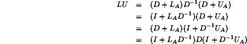
The first and fourth formulae are not suitable since they require
both multiplication and division with
; the difference between the
second and third is only one of ease of coding. In this section we use
the third formula; in the next section we will use the
second for the transpose system solution.
Both halves of the solution have largely the same structure as the
matrix vector multiplication.
for i = 1, n
sum = 0
for j = row_ptr(i), diag_ptr(i)-1
sum = sum + val(j) * z(col_ind(j))
end;
z(i) = pivots(i) * (x(i)-sum)
end;
for i = n, 1, (step -1)
sum = 0
for j = diag(i)+1, row_ptr(i+1)-1
sum = sum + val(j) * y(col_ind(j))
y(i) = z(i) - pivots(i) * sum
end;
end;
The temporary vector z can be eliminated by reusing the space
for y; algorithmically, z can even overwrite x, but overwriting input data is in general not recommended
.
Jack Dongarra
Mon Nov 20 08:52:54 EST 1995
CRS-based Factorization Transpose Solve
Next:
Generating a CRS-based
Up:
Sparse Incomplete Factorizations
Previous:
CRS-based Factorization Solve
Solving the transpose system  is slightly more involved. In the usual
formulation we traverse rows when solving a factored system, but here
we can only access columns of the matrices
is slightly more involved. In the usual
formulation we traverse rows when solving a factored system, but here
we can only access columns of the matrices  and
and  (at less
than prohibitive cost). The key idea is to distribute
each newly computed component of a triangular solve immediately over
the remaining right-hand-side.
(at less
than prohibitive cost). The key idea is to distribute
each newly computed component of a triangular solve immediately over
the remaining right-hand-side.
For instance, if we write a lower triangular matrix as
 , then the system
  can be written as
 . Hence, after computing
  we modify
 , and so on. Upper triangular systems are
treated in a similar manner.
With this algorithm we only access columns of the triangular systems.
Solving a transpose system with a matrix stored in CRS format
essentially means that we access rows of
and
.
, and so on. Upper triangular systems are
treated in a similar manner.
With this algorithm we only access columns of the triangular systems.
Solving a transpose system with a matrix stored in CRS format
essentially means that we access rows of
and
.
The algorithm now becomes
for i = 1, n
x_tmp(i) = x(i)
end;
for i = 1, n
z(i) = x_tmp(i)
tmp = pivots(i) * z(i)
for j = diag_ptr(i)+1, row_ptr(i+1)-1
x_tmp(col_ind(j)) = x_tmp(col_ind(j)) - tmp * val(j)
end;
end;
for i = n, 1 (step -1)
y(i) = pivots(i) * z(i)
for j = row_ptr(i), diag_ptr(i)-1
z(col_ind(j)) = z(col_ind(j)) - val(j) * y(i)
end;
end;
The extra temporary x_tmp is used only for clarity, and can
be overlapped with z. Both x_tmp and z can be
considered to be equivalent to y. Overall, a CRS-based
preconditioner solve uses short vector lengths, indirect addressing,
and has essentially the same memory traffic patterns as that of
the matrix-vector product.
Jack Dongarra
Mon Nov 20 08:52:54 EST 1995
Generating a CRS-based <IMG ALIGN=BOTTOM SRC="http://www.netlib.org/utk/papers/templates/_22900_tex2html_wrap7433.gif">
Incomplete Factorization
Next:
Parallelism
Up:
Sparse Incomplete Factorizations
Previous:
CRS-based Factorization Transpose
Incomplete factorizations with several levels of fill allowed are more
accurate than the
-
factorization described above. On the
other hand, they require more storage, and are considerably harder to
implement (much of this section is based on algorithms for a full
factorization of a sparse matrix as found in Duff, Erisman and
Reid
[80]).
As a preliminary, we need an algorithm for adding two vectors
and
, both stored in sparse storage. Let lx be the number
of nonzero components in
, let
be stored in x, and let
xind be an integer array such that

Similarly,
is stored as ly, y, yind.
We now add 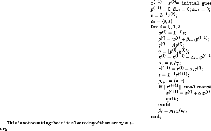 by first copying y into
a full vector w then adding w to x. The total number
of operations will be
by first copying y into
a full vector w then adding w to x. The total number
of operations will be  :
:
% copy y into w
for i=1,ly
w( yind(i) ) = y(i)
% add w to x wherever x is already nonzero
for i=1,lx
if w( xind(i) ) <> 0
x(i) = x(i) + w( xind(i) )
w( xind(i) ) = 0
% add w to x by creating new components
% wherever x is still zero
for i=1,ly
if w( yind(i) ) <> 0 then
lx = lx+1
xind(lx) = yind(i)
x(lx) = w( yind(i) )
endif
In order to add a sequence of vectors
 , we add the
 vectors into
  before executing
the writes into
.
A different implementation would be possible, where
is allocated
as a sparse vector and its sparsity pattern is constructed during the
additions. We will not discuss this possibility any further.
before executing
the writes into
.
A different implementation would be possible, where
is allocated
as a sparse vector and its sparsity pattern is constructed during the
additions. We will not discuss this possibility any further.
For a slight refinement of the above algorithm,
we will add levels to the nonzero components:
we assume integer vectors xlev and ylev of length lx
and ly respectively, and a full length level vector wlev
corresponding to w. The addition algorithm then becomes:
% copy y into w
for i=1,ly
w( yind(i) ) = y(i)
wlev( yind(i) ) = ylev(i)
% add w to x wherever x is already nonzero;
% don't change the levels
for i=1,lx
if w( xind(i) ) <> 0
x(i) = x(i) + w( xind(i) )
w( xind(i) ) = 0
% add w to x by creating new components
% wherever x is still zero;
% carry over levels
for i=1,ly
if w( yind(i) ) <> 0 then
lx = lx+1
x(lx) = w( yind(i) )
xind(lx) = yind(i)
xlev(lx) = wlev( yind(i) )
endif
We can now describe the  factorization. The algorithm starts
out with the matrix A, and gradually builds up
a factorization M of the form
factorization. The algorithm starts
out with the matrix A, and gradually builds up
a factorization M of the form  , where
,
, where
,
 , and
, and  are stored in the lower triangle, diagonal and
upper triangle of the array M respectively. The particular form
of the factorization is chosen to minimize the number of times that
the full vector w is copied back to sparse form.
are stored in the lower triangle, diagonal and
upper triangle of the array M respectively. The particular form
of the factorization is chosen to minimize the number of times that
the full vector w is copied back to sparse form.
Specifically, we use a sparse form of the following factorization
scheme:
for k=1,n
for j=1,k-1
for i=j+1,n
a(k,i) = a(k,i) - a(k,j)*a(j,i)
for j=k+1,n
a(k,j) = a(k,j)/a(k,k)
This is a row-oriented version of the traditional `left-looking'
factorization algorithm.
We will describe an incomplete factorization that controls fill-in
through levels (see equation (
)). Alternatively we
could use a drop tolerance (section
), but this is less
attractive from a point of implementation. With fill levels we can
perform the factorization symbolically at first, determining storage
demands and reusing this information through a number of linear
systems of the same sparsity structure. Such preprocessing and reuse
of information is not possible with fill controlled by a drop
tolerance criterion.
The matrix
arrays A and M are assumed to be in compressed row
storage, with no particular ordering of the elements inside each row,
but arrays adiag and mdiag point to the locations of the
diagonal elements.
for row=1,n
% go through elements A(row,col) with col<row
COPY ROW row OF A() INTO DENSE VECTOR w
for col=aptr(row),aptr(row+1)-1
if aind(col) < row then
acol = aind(col)
MULTIPLY ROW acol OF M() BY A(col)
SUBTRACT THE RESULT FROM w
ALLOWING FILL-IN UP TO LEVEL k
endif
INSERT w IN ROW row OF M()
% invert the pivot
M(mdiag(row)) = 1/M(mdiag(row))
% normalize the row of U
for col=mptr(row),mptr(row+1)-1
if mind(col) > row
M(col) = M(col) * M(mdiag(row))
The structure of a particular sparse matrix is likely to apply to a
sequence of problems, for instance on different time-steps, or during
a Newton iteration. Thus it may pay off to perform the above
incomplete factorization first symbolically to determine the amount
and location of fill-in and use this structure for the numerically
different but structurally identical matrices. In this case, the
array for the numerical values can be used to store the levels during
the symbolic factorization phase.
Next:
Parallelism
Up:
Sparse Incomplete Factorizations
Previous:
CRS-based Factorization Transpose
Jack Dongarra
Mon Nov 20 08:52:54 EST 1995
Parallelism
Next:
Inner products
Up:
Related Issues
Previous:
Generating a CRS-based
Pipelining: See: Vector computer.
Vector computer: Computer that is able to process
consecutive identical operations (typically additions or multiplications)
several times faster than intermixed operations of different types.
Processing identical operations this way is called `pipelining'
the operations.
Shared memory: See: Parallel computer.
Distributed memory: See: Parallel computer.
Message passing: See: Parallel computer.
Parallel computer: Computer with multiple independent
processing units. If the processors have immediate access to the
same memory, the memory is said to be shared; if processors have
private memory that is not immediately visible to other processors,
the memory is said to be distributed. In that case, processors
communicate by message passing.
In this section we discuss aspects of parallelism in the
iterative methods discussed in this book.
Since the iterative methods share most of their computational kernels
we will discuss these independent of the method.
The basic time-consuming kernels of iterative schemes are:
- inner products,
- vector updates,
- matrix-vector products, e.g.,
 (for some methods also
  ),
),
- preconditioner solves.
We will examine each of these in turn. We will conclude this section
by discussing two particular issues, namely computational wavefronts
in the SOR method,
and block operations in the GMRES method.
Jack Dongarra
Mon Nov 20 08:52:54 EST 1995
Inner products
Next:
Overlapping communication and
Up:
Parallelism
Previous:
Parallelism
The computation of an inner product of two vectors
can be easily parallelized; each processor computes the
inner product of corresponding segments of each vector
(local inner products or LIPs).
On distributed-memory machines the LIPs then
have to be sent to other processors
to be combined for the global inner product. This can be done either
with an all-to-all send where every processor performs the summation
of the LIPs, or by a global accumulation in one processor, followed by
a broadcast of the final result.
Clearly, this step requires communication.
For shared-memory machines, the accumulation of LIPs can be
implemented as a critical section where all processors add their local
result in turn to the global result, or as a piece of serial
code, where one processor performs the summations.
Jack Dongarra
Mon Nov 20 08:52:54 EST 1995
Overlapping communication and computation
Next:
Fewer synchronization points
Up:
Inner products
Previous:
Inner products
Clearly, in the usual formulation of conjugate gradient-type methods
the inner products induce a synchronization of the
processors, since they cannot progress until the final result has been
computed:
updating  and
and  can only begin after
completing the inner product for
can only begin after
completing the inner product for  . Since on a
distributed-memory machine communication is needed for the inner product, we
cannot overlap this communication with useful computation.
The same observation applies to updating
. Since on a
distributed-memory machine communication is needed for the inner product, we
cannot overlap this communication with useful computation.
The same observation applies to updating  , which can only begin
after completing the inner product for
, which can only begin
after completing the inner product for  .
.
Figure
shows a variant of CG, in which all
communication time may be overlapped with useful computations. This
is just a reorganized version of the original CG scheme, and is
therefore precisely as stable. Another advantage over other
approaches (see below) is that no additional operations are required.
This rearrangement is based on two tricks. The first is that updating
the iterate is delayed to mask the communication stage of the
 inner product. The second trick relies on splitting the
(symmetric) preconditioner as
inner product. The second trick relies on splitting the
(symmetric) preconditioner as  , so one first computes
 , after which the inner product
 can be computed as
  where
where  . The
computation of
. The
computation of  will then mask the communication stage of the
inner product.
will then mask the communication stage of the
inner product.

Figure: A rearrangement of Conjugate Gradient for parallelism
Under the assumptions that we have made, CG can be efficiently parallelized
as follows:
- The communication required for the reduction of the inner
product for
 can be overlapped with the update for
  ,
(which could in fact have been done in the previous iteration step).
,
(which could in fact have been done in the previous iteration step).
- The reduction of the inner product for
 can be
overlapped with the remaining part of the preconditioning operation
at the beginning of the next iteration.
can be
overlapped with the remaining part of the preconditioning operation
at the beginning of the next iteration.
- The computation of a segment of
can be followed
immediately by the computation of a segment of
 , and this can
be followed by the computation of a part of the inner product. This
saves on load operations for segments of
and
.
, and this can
be followed by the computation of a part of the inner product. This
saves on load operations for segments of
and
.
For a more detailed discussion see Demmel, Heath and
Van der Vorst
[67]. This algorithm
can be extended trivially to preconditioners of  form, and
nonsymmetric preconditioners in the Biconjugate Gradient Method.
form, and
nonsymmetric preconditioners in the Biconjugate Gradient Method.
Next:
Fewer synchronization points
Up:
Inner products
Previous:
Inner products
Jack Dongarra
Mon Nov 20 08:52:54 EST 1995
Fewer synchronization points
Next:
Vector updates
Up:
Inner products
Previous:
Overlapping communication and
Several authors have found ways to eliminate some of the
synchronization points induced by the
inner products in methods such as CG. One strategy has been to
replace one of the two inner products typically present in conjugate
gradient-like methods by one or two others in such a way that all
inner products can be performed simultaneously. The global
communication can then be packaged. A first such method was proposed
by Saad
[182] with a modification to improve its
stability suggested by Meurant
[156]. Recently, related
methods have been
proposed by Chronopoulos and Gear
[55], D'Azevedo and
Romine
[62], and Eijkhout
[88].
These schemes can also be applied to
nonsymmetric methods such as BiCG. The stability of such methods is
discussed by D'Azevedo, Eijkhout and Romine
[61].
Another approach is to generate a number of
successive Krylov vectors (see §
) and
orthogonalize these as a block (see
Van Rosendale
[210], and Chronopoulos and
Gear
[55]).
Jack Dongarra
Mon Nov 20 08:52:54 EST 1995
Vector updates
Next:
Matrix-vector products
Up:
Parallelism
Previous:
Fewer synchronization points
Vector updates are trivially parallelizable: each processor updates its
own segment.
Jack Dongarra
Mon Nov 20 08:52:54 EST 1995
Stationary Iterative Methods
Next:
The Jacobi Method
Up:
Iterative Methods
Previous:
Overview of the
Iterative methods that can be expressed in the simple form

(where neither  nor
nor  depend upon the iteration count
) are
called stationary iterative methods.
In this section, we present the four main stationary iterative
methods: the Jacobi
method, the Gauss-Seidel
method, the Successive
Overrelaxation
(SOR) method and
the Symmetric Successive Overrelaxation
(SSOR) method.
In each case,
we summarize their convergence behavior and their effectiveness, and
discuss how and when they should be used. Finally,
in §
, we give some historical background and
further notes and references.
depend upon the iteration count
) are
called stationary iterative methods.
In this section, we present the four main stationary iterative
methods: the Jacobi
method, the Gauss-Seidel
method, the Successive
Overrelaxation
(SOR) method and
the Symmetric Successive Overrelaxation
(SSOR) method.
In each case,
we summarize their convergence behavior and their effectiveness, and
discuss how and when they should be used. Finally,
in §
, we give some historical background and
further notes and references.
Jack Dongarra
Mon Nov 20 08:52:54 EST 1995
Matrix-vector products
Next:
Preconditioning
Up:
Parallelism
Previous:
Vector updates
The matrix-vector products are often easily parallelized on shared-memory
machines by splitting the matrix in strips corresponding to the vector
segments. Each processor then computes the matrix-vector product of one
strip.
For distributed-memory machines, there may be a problem if each processor
has only a segment of the vector in its memory. Depending on the bandwidth
of the matrix, we may need communication for other elements of the vector,
which may lead to communication bottlenecks. However, many sparse
matrix problems arise from a network in which only nearby nodes are
connected. For example, matrices stemming
from finite difference or finite element problems typically involve
only local connections: matrix element
is nonzero
only if variables  and
and  are physically close.
In such a case, it seems natural to subdivide the network, or
grid, into suitable blocks and to distribute them over the processors.
When computing
are physically close.
In such a case, it seems natural to subdivide the network, or
grid, into suitable blocks and to distribute them over the processors.
When computing  , each processor requires the values of
  at
some nodes in neighboring blocks. If the number of connections to these
neighboring blocks is small compared to the number of internal nodes,
then the communication time can be overlapped with computational work.
For more detailed discussions on implementation aspects for distributed
memory systems, see De Sturler
[63] and
Pommerell
[175].
at
some nodes in neighboring blocks. If the number of connections to these
neighboring blocks is small compared to the number of internal nodes,
then the communication time can be overlapped with computational work.
For more detailed discussions on implementation aspects for distributed
memory systems, see De Sturler
[63] and
Pommerell
[175].
Jack Dongarra
Mon Nov 20 08:52:54 EST 1995
Preconditioning
Next:
Discovering parallelism in
Up:
Parallelism
Previous:
Matrix-vector products
Preconditioning is often the most problematic part of parallelizing
an iterative method.
We will mention a number of approaches to obtaining parallelism in
preconditioning.
Jack Dongarra
Mon Nov 20 08:52:54 EST 1995
Discovering parallelism in sequential preconditioners.
Next:
More parallel variants
Up:
Preconditioning
Previous:
Preconditioning
Certain preconditioners were not developed with parallelism in mind,
but they can be executed in parallel. Some examples are domain
decomposition methods (see §
), which
provide a high degree of coarse grained parallelism,
and polynomial preconditioners
(see §
), which have the same parallelism as
the matrix-vector product.
Incomplete factorization preconditioners are usually much harder to
parallelize: using wavefronts of independent computations (see for
instance Paolini and Radicati di Brozolo
[170]) a
modest amount of parallelism
can be attained, but the implementation is complicated. For instance,
a central difference discretization on regular grids gives wavefronts
that are hyperplanes
(see Van der Vorst
[205]
[203]).
Jack Dongarra
Mon Nov 20 08:52:54 EST 1995
More parallel variants of sequential preconditioners.
Next:
Fully decoupled preconditioners.
Up:
Preconditioning
Previous:
Discovering parallelism in
Variants of existing sequential incomplete factorization
preconditioners with a higher degree of parallelism have been devised,
though they are perhaps less efficient in purely scalar terms than
their ancestors. Some examples are: reorderings of the
variables (see Duff and Meurant
[79] and
Eijkhout
[85]), expansion of the
factors in a truncated Neumann series (see
Van der Vorst
[201]),
various block factorization methods (see
Axelsson and Eijkhout
[15]
and
Axelsson and Polman
[21]),
and multicolor preconditioners.
Multicolor preconditioners have optimal parallelism among incomplete
factorization methods, since the minimal number of sequential steps
equals the color number of the matrix graphs. For theory and
applications to parallelism
see Jones and Plassman
[128]
[127].
Jack Dongarra
Mon Nov 20 08:52:54 EST 1995
Fully decoupled preconditioners.
Next:
Wavefronts in the
Up:
Preconditioning
Previous:
More parallel variants
If all processors execute their part of the preconditioner solve
without further communication, the overall method is technically a
block Jacobi preconditioner (see §
).
While their parallel execution is very efficient, they
may not be as effective as more complicated, less parallel
preconditioners, since improvement in the number of iterations
may be only modest.
To get a bigger improvement while retaining the efficient parallel
execution,
Radicati di Brozolo and Robert
[178] suggest that one construct
incomplete decompositions on slightly overlapping domains. This requires
communication similar to that for matrix-vector products.
Jack Dongarra
Mon Nov 20 08:52:54 EST 1995
Wavefronts in the Gauss-Seidel and Conjugate Gradient methods
Next:
Blocked operations in
Up:
Parallelism
Previous:
Fully decoupled preconditioners.
At first sight, the Gauss-Seidel method (and the SOR method which has
the same basic structure) seems to be a fully sequential method.
A more careful analysis, however, reveals a high degree of parallelism
if the method is applied to sparse matrices such as those arising from
discretized partial differential equations.
We start by partitioning the unknowns in wavefronts. The first
wavefront contains those unknowns that (in the directed graph of
 ) have no predecessor; subsequent wavefronts are then sets (this
definition is not necessarily unique) of successors of elements of the
previous wavefront(s), such that no successor/predecessor relations hold
among the elements of this set. It is clear that all elements of a
wavefront can be processed simultaneously, so the sequential time of
solving a system with
can be reduced to the number of
wavefronts.
) have no predecessor; subsequent wavefronts are then sets (this
definition is not necessarily unique) of successors of elements of the
previous wavefront(s), such that no successor/predecessor relations hold
among the elements of this set. It is clear that all elements of a
wavefront can be processed simultaneously, so the sequential time of
solving a system with
can be reduced to the number of
wavefronts.
Next, we observe that the unknowns in a wavefront can be computed as
soon as all wavefronts containing its predecessors have been computed.
Thus we can, in the absence of tests for convergence, have components
from several iterations being computed simultaneously.
Adams and Jordan
[2] observe that in this way
the natural ordering of unknowns gives an iterative method that is
mathematically equivalent to a multi-color ordering.
In the multi-color ordering, all wavefronts of the same color are
processed simultaneously. This reduces the number of sequential steps
for solving the Gauss-Seidel matrix to the number of colors, which is
the smallest number  such that wavefront
contains no
elements that are a predecessor of an element in wavefront
such that wavefront
contains no
elements that are a predecessor of an element in wavefront  .
.
As demonstrated by O'Leary
[164], SOR theory still holds
in an approximate sense for multi-colored matrices. The above
observation that the Gauss-Seidel method with the natural ordering is
equivalent to a multicoloring cannot be extended to the SSOR method or
wavefront-based incomplete factorization preconditioners for the
Conjugate Gradient method. In fact, tests by Duff and
Meurant
[79] and
an analysis by Eijkhout
[85] show that multicolor incomplete
factorization preconditioners in general may take a considerably
larger number of iterations to converge than preconditioners based on
the natural ordering. Whether this is offset by the increased
parallelism depends on the application and the computer architecture.
Next:
Blocked operations in
Up:
Parallelism
Previous:
Fully decoupled preconditioners.
Jack Dongarra
Mon Nov 20 08:52:54 EST 1995
Blocked operations in the GMRES method
Next:
Remaining topics
Up:
Parallelism
Previous:
Wavefronts in the
In addition to the usual matrix-vector product, inner products and
vector updates, the preconditioned GMRES method
(see §
) has a kernel where one new vector,
 , is orthogonalized against the previously built
orthogonal set {
, is orthogonalized against the previously built
orthogonal set { ,
,  ,...,
,...,  }.
In our version, this is
done using Level 1 BLAS, which may be quite inefficient. To
incorporate Level 2 BLAS we can apply either Householder
orthogonalization or classical Gram-Schmidt twice (which mitigates
classical Gram-Schmidt's potential instability; see
Saad
[185]). Both
approaches significantly increase the computational work, but using
classical Gram-Schmidt has the advantage that all inner products can
be performed simultaneously; that is, their communication can be
packaged. This may increase the efficiency of the computation
significantly.
}.
In our version, this is
done using Level 1 BLAS, which may be quite inefficient. To
incorporate Level 2 BLAS we can apply either Householder
orthogonalization or classical Gram-Schmidt twice (which mitigates
classical Gram-Schmidt's potential instability; see
Saad
[185]). Both
approaches significantly increase the computational work, but using
classical Gram-Schmidt has the advantage that all inner products can
be performed simultaneously; that is, their communication can be
packaged. This may increase the efficiency of the computation
significantly.
Another way to obtain more parallelism and
data locality is to generate a basis
{
,  , ...,
  } for the Krylov subspace first,
and to orthogonalize this set afterwards; this is called
} for the Krylov subspace first,
and to orthogonalize this set afterwards; this is called
 -step GMRES(
) (see Kim and Chronopoulos
[139]).
(Compare this to the GMRES method in §
, where each
new vector is immediately orthogonalized to all previous vectors.)
This approach does not
increase the computational work and, in contrast to CG, the numerical
instability due to generating a possibly near-dependent set is not
necessarily a drawback.
-step GMRES(
) (see Kim and Chronopoulos
[139]).
(Compare this to the GMRES method in §
, where each
new vector is immediately orthogonalized to all previous vectors.)
This approach does not
increase the computational work and, in contrast to CG, the numerical
instability due to generating a possibly near-dependent set is not
necessarily a drawback.
Jack Dongarra
Mon Nov 20 08:52:54 EST 1995
Remaining topics
Next:
The Lanczos Connection
Up:
Templates for the Solution
Previous:
Blocked operations in
Jack Dongarra
Mon Nov 20 08:52:54 EST 1995
The Lanczos Connection
Next:
Block and -step
Up:
Remaining topics
Previous:
Remaining topics
As discussed by Paige and Saunders in
[168] and by
Golub and Van Loan in
[109], it is straightforward to
derive the conjugate gradient method for solving symmetric positive
definite linear systems from the Lanczos algorithm for solving
symmetric eigensystems and vice versa. As an example, let us consider
how one can derive the Lanczos process for symmetric eigensystems from
the (unpreconditioned) conjugate gradient method.
Suppose we define the  matrix
  by
by

and the  upper bidiagonal matrix
  by
by
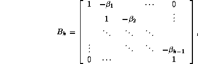
where the sequences  and
and  are defined by the standard
conjugate gradient algorithm discussed in §
.
From the equations
are defined by the standard
conjugate gradient algorithm discussed in §
.
From the equations

and  , we have
  , where

Assuming the elements of the sequence  are
-conjugate,
it follows that
are
-conjugate,
it follows that

is a tridiagonal matrix since
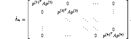
Since span{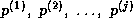 } =
span{
} =
span{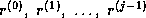 } and since the elements of
 are mutually orthogonal, it can be shown that the columns of
matrix
are mutually orthogonal, it can be shown that the columns of
matrix  form an orthonormal basis
for the subspace
form an orthonormal basis
for the subspace 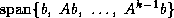 , where
 is a diagonal matrix whose
th diagonal element is
is a diagonal matrix whose
th diagonal element is  . The columns of the matrix
  are the Lanczos vectors (see
Parlett
[171]) whose associated projection of
is
the tridiagonal matrix
are the Lanczos vectors (see
Parlett
[171]) whose associated projection of
is
the tridiagonal matrix

The extremal eigenvalues of  approximate those of the
matrix
. Hence,
the diagonal and subdiagonal elements of
in
(
), which are readily available during iterations of the
conjugate gradient algorithm (§
),
can be used to construct
after
CG iterations. This
allows us to obtain good approximations to the extremal eigenvalues
(and hence the condition number) of the matrix
while we are generating
approximations,
approximate those of the
matrix
. Hence,
the diagonal and subdiagonal elements of
in
(
), which are readily available during iterations of the
conjugate gradient algorithm (§
),
can be used to construct
after
CG iterations. This
allows us to obtain good approximations to the extremal eigenvalues
(and hence the condition number) of the matrix
while we are generating
approximations,  , to the solution of the linear system
.
, to the solution of the linear system
.
For a nonsymmetric matrix
, an equivalent nonsymmetric Lanczos
algorithm (see Lanczos
[142]) would produce a
nonsymmetric matrix
in (
) whose extremal eigenvalues
(which may include complex-conjugate pairs) approximate those of
.
The nonsymmetric Lanczos method is equivalent to the BiCG method
discussed in §
.
Next:
Block and -step
Up:
Remaining topics
Previous:
Remaining topics
Jack Dongarra
Mon Nov 20 08:52:54 EST 1995
Block and <IMG ALIGN=BOTTOM SRC="http://www.netlib.org/utk/papers/templates/_22900_tex2html_wrap7625.gif">
-step Iterative Methods
Next:
Reduced System Preconditioning
Up:
Remaining topics
Previous:
The Lanczos Connection
The methods discussed so far are all subspace methods, that is, in
every iteration they extend the dimension of the subspace generated. In
fact, they generate an orthogonal basis for this subspace, by
orthogonalizing the newly generated vector with respect to the
previous basis vectors.
However, in the case of nonsymmetric coefficient matrices the newly
generated vector may be almost linearly dependent on the existing
basis. To prevent break-down or severe numerical error in such
instances, methods have been proposed that perform a look-ahead step
(see Freund, Gutknecht and
Nachtigal
[101], Parlett, Taylor and
Liu
[172], and Freund and
Nachtigal
[102]).
Several new, unorthogonalized, basis
vectors are generated and are then orthogonalized with
respect to the subspace already generated. Instead of generating a
basis, such a method generates a series of low-dimensional orthogonal
subspaces.
The  -step iterative methods of Chronopoulos and
Gear
[55] use this strategy of generating
unorthogonalized vectors and processing them as a block to reduce
computational overhead and improve processor cache behavior.
-step iterative methods of Chronopoulos and
Gear
[55] use this strategy of generating
unorthogonalized vectors and processing them as a block to reduce
computational overhead and improve processor cache behavior.
If conjugate gradient methods are considered to generate a
factorization of a tridiagonal reduction of the original matrix, then
look-ahead methods generate a block factorization of a block
tridiagonal reduction of the matrix.
A block tridiagonal reduction is also effected by the
Block Lanczos algorithm and the Block Conjugate Gradient
method
(see O'Leary
[163]).
Such methods operate on multiple linear systems with the same
coefficient matrix simultaneously, for instance with multiple right hand
sides, or the same right hand side but with different initial guesses.
Since these block methods use multiple search directions in each step,
their convergence behavior is better than for ordinary methods. In fact,
one can show that the spectrum of the matrix is effectively
reduced by the  smallest eigenvalues, where
  is the block
size.
is the block
size.
Next:
Reduced System Preconditioning
Up:
Remaining topics
Previous:
The Lanczos Connection
Jack Dongarra
Mon Nov 20 08:52:54 EST 1995
The Jacobi Method
Next:
Convergence of the
Up:
Stationary Iterative Methods
Previous:
Stationary Iterative Methods
The Jacobi method is easily derived by examining each of
the
equations in the linear system
in isolation. If in
the
th equation

we solve for the value of  while assuming the other entries
of
remain fixed, we obtain
while assuming the other entries
of
remain fixed, we obtain

This suggests an iterative method defined by

which is the Jacobi method. Note that the order in which the
equations are examined is irrelevant, since the Jacobi method treats
them independently. For this reason, the Jacobi method is also known
as the method of simultaneous displacements, since the updates
could in principle be done simultaneously.
Simultaneous displacements, method of: Jacobi method.
In matrix terms, the definition of the Jacobi method
in (
) can be expressed as

where the matrices
,  and
and  represent the diagonal, the
strictly lower-triangular, and the strictly upper-triangular parts of
,
respectively.
represent the diagonal, the
strictly lower-triangular, and the strictly upper-triangular parts of
,
respectively.
The pseudocode for the Jacobi method is given in Figure
.
Note that an auxiliary storage vector,  is used in the
algorithm. It is not possible to update the vector
in place,
since values from
is used in the
algorithm. It is not possible to update the vector
in place,
since values from  are needed throughout the
computation of
.
are needed throughout the
computation of
.
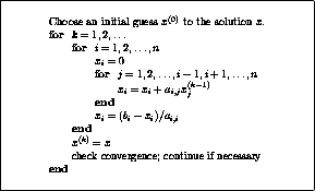
Figure: The Jacobi Method
Jack Dongarra
Mon Nov 20 08:52:54 EST 1995
Reduced System Preconditioning
Next:
Domain Decomposition Methods
Up:
Remaining topics
Previous:
Block and -step
Reduced system: Linear system obtained by eliminating
certain variables from another linear system.
Although the number of variables is smaller
than for the original system, the matrix of a reduced system generally
has more nonzero entries. If the original matrix was symmetric and positive
definite, then the reduced system has a smaller condition number.
As we have seen earlier, a suitable preconditioner for CG is a
matrix
such that the system

requires fewer iterations to solve than  does, and for which
systems
does, and for which
systems  can be solved efficiently. The first property is
independent of the machine used, while the second is highly machine
dependent. Choosing the best preconditioner involves balancing those
two criteria in a way that minimizes the overall computation time.
One balancing approach used for matrices
arising from
can be solved efficiently. The first property is
independent of the machine used, while the second is highly machine
dependent. Choosing the best preconditioner involves balancing those
two criteria in a way that minimizes the overall computation time.
One balancing approach used for matrices
arising from  -point
finite difference discretization of second order elliptic partial
differential equations (PDEs) with Dirichlet boundary conditions
involves solving a reduced system. Specifically, for an
grid, we can use a point red-black ordering of the nodes to
get
-point
finite difference discretization of second order elliptic partial
differential equations (PDEs) with Dirichlet boundary conditions
involves solving a reduced system. Specifically, for an
grid, we can use a point red-black ordering of the nodes to
get

where  and
and  are diagonal, and
  is a well-structured
sparse matrix with
nonzero diagonals if
is even and
is a well-structured
sparse matrix with
nonzero diagonals if
is even and
 nonzero diagonals if
is odd. Applying one step
of block Gaussian elimination (or computing the
Schur complement; see Golub and Van Loan
[109]) we have
nonzero diagonals if
is odd. Applying one step
of block Gaussian elimination (or computing the
Schur complement; see Golub and Van Loan
[109]) we have

which reduces to

With proper scaling (left and right multiplication by  ),
we obtain from the second block equation the reduced system
),
we obtain from the second block equation the reduced system

where  ,
,  , and
, and  . The linear system (
) is of
order
. The linear system (
) is of
order  for even
and of order
for even
and of order  for odd
. Once
is determined, the solution
is easily retrieved from
. The
values on the black points are those that would be obtained from a
red/black ordered SSOR preconditioner on the full system, so we expect
faster convergence.
for odd
. Once
is determined, the solution
is easily retrieved from
. The
values on the black points are those that would be obtained from a
red/black ordered SSOR preconditioner on the full system, so we expect
faster convergence.
The number of nonzero coefficients is reduced, although the
coefficient matrix in (
) has nine nonzero diagonals.
Therefore it has higher density and offers more data locality.
Meier and Sameh
[150] demonstrate that the reduced system
approach on hierarchical memory
machines such as the Alliant FX/8 is over
 times faster than unpreconditioned CG for Poisson's equation on
grids with
times faster than unpreconditioned CG for Poisson's equation on
grids with  .
.
For
-dimensional elliptic PDEs, the reduced system approach yields
a block tridiagonal matrix
in (
) having diagonal
blocks of the structure of
from the  -dimensional case and
off-diagonal blocks that are diagonal matrices. Computing the reduced
system explicitly leads to an unreasonable increase in the
computational complexity of solving
. The matrix products
required to solve (
) would therefore be performed implicitly
which could significantly decrease performance. However, as Meier and
Sameh show
[150], the reduced system approach can still be about
-
times as fast as the conjugate gradient method with Jacobi
preconditioning for
-dimensional problems.
-dimensional case and
off-diagonal blocks that are diagonal matrices. Computing the reduced
system explicitly leads to an unreasonable increase in the
computational complexity of solving
. The matrix products
required to solve (
) would therefore be performed implicitly
which could significantly decrease performance. However, as Meier and
Sameh show
[150], the reduced system approach can still be about
-
times as fast as the conjugate gradient method with Jacobi
preconditioning for
-dimensional problems.
Domain decomposition method: Solution method for
linear systems based on a partitioning of the physical domain
of the differential equation. Domain decomposition methods typically
involve (repeated) independent system solution on the subdomains,
and some way of combining data from the subdomains on the separator
part of the domain.
Next:
Domain Decomposition Methods
Up:
Remaining topics
Previous:
Block and -step
Jack Dongarra
Mon Nov 20 08:52:54 EST 1995
Domain Decomposition Methods
Next:
Overlapping Subdomain Methods
Up:
Remaining topics
Previous:
Reduced System Preconditioning
In recent years, much attention has been given to domain decomposition
methods for linear elliptic problems that are based on a partitioning
of the domain of the physical problem. Since the subdomains can be
handled independently, such methods are very attractive for
coarse-grain parallel computers. On the other hand, it should be
stressed that they can be very effective even on sequential computers.
In this brief survey, we shall restrict ourselves to the standard
second order self-adjoint scalar elliptic problems in two dimensions
of the form:

where  is a positive function on the domain
  , on whose
boundary the value of
, on whose
boundary the value of  is prescribed (the Dirichlet problem). For
more general problems, and a good set of references, the reader is
referred to the series of
proceedings
[177]
[135]
[107]
[49]
[48]
[47]
and the surveys
[196]
[51].
is prescribed (the Dirichlet problem). For
more general problems, and a good set of references, the reader is
referred to the series of
proceedings
[177]
[135]
[107]
[49]
[48]
[47]
and the surveys
[196]
[51].
For the discretization of (
), we shall assume for
simplicity that
is triangulated by a set  of nonoverlapping
coarse triangles (subdomains)
of nonoverlapping
coarse triangles (subdomains)  with
with  internal
vertices. The
internal
vertices. The  's are in turn
further refined into a set of smaller triangles
's are in turn
further refined into a set of smaller triangles  with
internal vertices in total.
Here
with
internal vertices in total.
Here  denote the coarse and fine mesh size respectively.
By a standard Ritz-Galerkin method using piecewise linear triangular
basis elements on (
), we obtain an
symmetric positive definite linear system
denote the coarse and fine mesh size respectively.
By a standard Ritz-Galerkin method using piecewise linear triangular
basis elements on (
), we obtain an
symmetric positive definite linear system
 .
.
Generally, there are two kinds of approaches depending on whether
the subdomains overlap with one another
(Schwarz methods
) or are separated from
one another by interfaces (Schur Complement methods
,
iterative substructuring).
We shall present domain decomposition methods as preconditioners
for the linear system
to
a reduced (Schur Complement) system
 defined on the interfaces in the non-overlapping formulation.
When used with the standard Krylov subspace methods discussed
elsewhere in this book, the user has to supply a procedure
for computing
defined on the interfaces in the non-overlapping formulation.
When used with the standard Krylov subspace methods discussed
elsewhere in this book, the user has to supply a procedure
for computing  or
or  given
given  or
and the algorithms to be described
herein computes
or
and the algorithms to be described
herein computes  .
The computation of
is a simple sparse matrix-vector
multiply, but
may require subdomain solves, as will be described later.
.
The computation of
is a simple sparse matrix-vector
multiply, but
may require subdomain solves, as will be described later.
Next:
Overlapping Subdomain Methods
Up:
Remaining topics
Previous:
Reduced System Preconditioning
Jack Dongarra
Mon Nov 20 08:52:54 EST 1995
Overlapping Subdomain Methods
Next:
Non-overlapping Subdomain Methods
Up:
Domain Decomposition Methods
Previous:
Domain Decomposition Methods
In this approach, each substructure
is extended to a
larger substructure  containing
  internal vertices and all the
triangles
internal vertices and all the
triangles  , within a distance
  from
, where
refers to the amount of overlap.
from
, where
refers to the amount of overlap.
Let  denote the the discretizations
of (
) on the subdomain
triangulation
denote the the discretizations
of (
) on the subdomain
triangulation  and the coarse triangulation
respectively.
and the coarse triangulation
respectively.
Let  denote the extension operator which extends (by zero) a
function on
to
and
denote the extension operator which extends (by zero) a
function on
to
and
 the corresponding pointwise restriction operator.
Similarly, let
the corresponding pointwise restriction operator.
Similarly, let  denote the interpolation operator
which maps a function on the coarse grid
onto the fine
grid
by piecewise linear interpolation
and
denote the interpolation operator
which maps a function on the coarse grid
onto the fine
grid
by piecewise linear interpolation
and  the corresponding weighted restriction operator.
With these notations, the Additive Schwarz Preconditioner  for
the system
can be compactly described as:
for
the system
can be compactly described as:
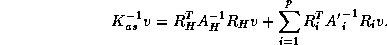
Note that the right hand side can be computed using

subdomain
solves using the

's, plus a coarse grid solve using

,
all of which can be computed in parallel.
Each term

should be evaluated in three steps:
(1) Restriction:

,
(2) Subdomain solves for

:

,
(3) Interpolation:

.
The coarse grid solve is handled in the same manner.
The theory of Dryja and Widlund
[76] shows that
the condition number of

is bounded independently
of both the coarse grid size

and the fine grid size

,
provided there is ``sufficient'' overlap between

and

(essentially it means that the ratio

of
the distance

of the boundary

to

should be uniformly bounded from below as

.)
If the coarse grid solve term is left out, then the
condition number grows as

, reflecting the lack
of global coupling provided by the coarse grid.
For the purpose of implementations, it is often useful to interpret
the definition of

in matrix notation.
Thus the decomposition of

into
's corresponds to partitioning
of the components of the vector

into
overlapping groups of
index sets

's, each with

components.
The

matrix
is simply a principal submatrix of

corresponding to the index set
.

is a

matrix
defined by its action on
a vector

defined on

as:

if

but is zero otherwise.
Similarly, the action of its transpose

forms an
-vector by picking
off the components of
corresponding to
.
Analogously,

is an

matrix
with entries corresponding to piecewise linear interpolation
and its transpose can be interpreted as a weighted restriction matrix.
If

is obtained from

by nested refinement,
the action of

can be efficiently computed
as in a standard multigrid algorithm.
Note that the matrices

are defined
by their actions and need not be stored explicitly.
We also note that in this algebraic formulation, the preconditioner
can be extended to any matrix
,
not necessarily one arising from a discretization of an elliptic problem.
Once we have the partitioning
index sets
's, the matrices

are defined.
Furthermore, if
is positive definite, then
is guaranteed
to be nonsingular. The difficulty is in defining the ``coarse grid''
matrices

, which inherently depends on knowledge of the
grid structure.
This part of the preconditioner can be left out, at the expense
of a deteriorating convergence rate as
increases.
Radicati and Robert
[178]
have experimented with such an algebraic overlapping block Jacobi
preconditioner.
Next:
Non-overlapping Subdomain Methods
Up:
Domain Decomposition Methods
Previous:
Domain Decomposition Methods
Jack Dongarra
Mon Nov 20 08:52:54 EST 1995
Non-overlapping Subdomain Methods
Next:
Further Remarks
Up:
Domain Decomposition Methods
Previous:
Overlapping Subdomain Methods
The easiest way to describe this approach is through
matrix notation.
The set of vertices of
can be divided into two groups.
The set of interior vertices  of
all
and the set of vertices
which lies on the boundaries
of
all
and the set of vertices
which lies on the boundaries
 of the coarse triangles
in
.
We shall re-order
and
of the coarse triangles
in
.
We shall re-order
and  as
as  and
and  corresponding to this partition.
In this ordering, equation (
) can be written
as follows:
corresponding to this partition.
In this ordering, equation (
) can be written
as follows:

We note that since the subdomains are uncoupled by the boundary vertices,
 is block-diagonal
with each block
is block-diagonal
with each block  being the stiffness matrix corresponding
to the unknowns belonging to the interior
vertices of subdomain
.
being the stiffness matrix corresponding
to the unknowns belonging to the interior
vertices of subdomain
.
By a block LU-factorization of
, the system in (
)
can be written as:

where

is the Schur complement of

in
.
By eliminating

in (
), we arrive at
the following equation for

:

We note the following properties of this Schur Complement system:
-

inherits the symmetric positive definiteness of
.
-
is dense in general and computing it explicitly
requires as many solves on each subdomain as there are
points on each of its edges.
- The condition number of
is

, an improvement
over the

growth for
.
- Given a vector

defined on the boundary vertices

of
,
the matrix-vector product

can be computed according to

where

involves
independent subdomain solves using

.
- The right hand side

can also be computed using
independent subdomain solves.
These properties make it possible
to apply a preconditioned iterative method to (
), which is
the basic method in the nonoverlapping substructuring approach.
We will also need some good preconditioners
to further improve the convergence of the Schur system.
We shall first describe
the Bramble-Pasciak-Schatz preconditioner
[36].
For this, we need to further decompose
into two non-overlapping
index sets:

where

denote the set of
nodes
corresponding to the vertices

's of
, and

denote the set of
nodes
on the edges

's
of the coarse triangles in
, excluding
the vertices
belonging to

.
In addition to the coarse grid interpolation and restriction
operators
defined before,
we shall also need a new set of interpolation and restriction
operators for the edges
's.
Let

be the pointwise restriction operator
(an

matrix, where

is the number
of vertices on the edge
)
onto the edge
defined by its action

if

but is zero otherwise.
The action of its transpose extends by zero a function
defined on
to one defined on
.
Corresponding to this partition of
,

can be written in
the block form:

The block

can again be block partitioned, with most of
the subblocks being zero. The diagonal blocks

of
are the
principal submatrices of
corresponding to
.
Each
represents the coupling of nodes on interface
separating two neighboring subdomains.
In defining the preconditioner, the action of

is
needed. However, as noted before, in general
is a dense
matrix which is also expensive to compute, and even if we had it, it
would be expensive to compute its action (we would need to compute its
inverse or a Cholesky factorization). Fortunately, many efficiently
invertible approximations to
have been proposed in the
literature (see Keyes and Gropp
[136]) and we shall use these
so-called interface preconditioners for
instead.
We mention one specific preconditioner:

where

is an

one dimensional
Laplacian matrix, namely a tridiagonal matrix with

's down
the main diagonal and

's down the two off-diagonals,
and

is taken to be some average of the coefficient

of (
) on the edge
.
We note that since the eigen-decomposition of
is known
and computable by the Fast Sine Transform, the action of

can be efficiently computed.
With these notations, the Bramble-Pasciak-Schatz preconditioner
is defined by its action on a vector
defined on
as follows:

Analogous to the additive Schwarz preconditioner,
the computation of each term consists of the three steps
of restriction-inversion-interpolation and
is independent of the others and thus can be carried out in parallel.
Bramble, Pasciak and Schatz
[36] prove that the condition
number of

is bounded by

. In
practice, there is a slight growth in the number of iterations as
becomes small (i.e., as the fine grid is refined) or as
becomes large (i.e., as the coarse grid becomes coarser).
The

growth is due to the coupling of the unknowns on the
edges incident on a common vertex
, which is not accounted for in

. Smith
[191] proposed a vertex space
modification to
which explicitly accounts for this coupling
and therefore eliminates the dependence on
and
. The idea is
to introduce further subsets of
called vertex spaces

with

consisting of a small set of vertices on
the edges incident on the vertex
and adjacent to it. Note that

overlaps with

and
. Let

be the principal
submatrix of
corresponding to
, and

be
the corresponding restriction (pointwise) and extension (by zero)
matrices. As before,
is dense and expensive to compute and
factor/solve but efficiently invertible approximations (some using
variants of the

operator defined before) have been developed
in the literature (see Chan, Mathew and
Shao
[52]). We shall let

be such a
preconditioner for
. Then Smith's Vertex Space
preconditioner is defined by:
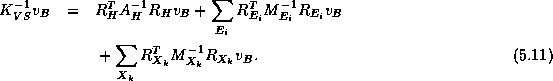
Smith
[191] proved that the condition number
of

is bounded independent of
and
, provided
there is sufficient overlap of
with
.
Next:
Further Remarks
Up:
Domain Decomposition Methods
Previous:
Overlapping Subdomain Methods
Jack Dongarra
Mon Nov 20 08:52:54 EST 1995
Further Remarks
Next:
Multiplicative Schwarz Methods
Up:
Domain Decomposition Methods
Previous:
Non-overlapping Subdomain Methods
Jack Dongarra
Mon Nov 20 08:52:54 EST 1995
Multiplicative Schwarz Methods
Next:
Inexact Solves
Up:
Further Remarks
Previous:
Further Remarks
As mentioned before,
the Additive Schwarz preconditioner can be
viewed as an overlapping block Jacobi preconditioner.
Analogously, one can define a multiplicative Schwarz
preconditioner which corresponds to a symmetric block Gauss-Seidel
version. That is, the solves on each subdomain are performed
sequentially, using the most current iterates as boundary conditions
from neighboring subdomains. Even without conjugate gradient
acceleration, the multiplicative
method can take many fewer iterations than the additive version.
However, the multiplicative version is not as parallelizable,
although the degree of parallelism can be increased
by trading off the convergence rate through
multi-coloring the subdomains.
The theory can be found in Bramble, et al.
[37].
Jack Dongarra
Mon Nov 20 08:52:54 EST 1995
Inexact Solves
Next:
Nonsymmetric Problems
Up:
Further Remarks
Previous:
Multiplicative Schwarz Methods
The exact solves involving  and
and  in
in
 can be replaced by inexact solves
 and
and  ,
which can be standard elliptic preconditioners themselves
(e.g. multigrid, ILU, SSOR, etc.).
,
which can be standard elliptic preconditioners themselves
(e.g. multigrid, ILU, SSOR, etc.).
For the Schwarz methods, the modification is straightforward
and the Inexact Solve Additive Schwarz Preconditioner
is simply:
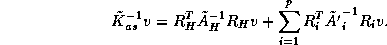
The Schur Complement methods require more changes to accommodate
inexact solves.
By replacing

by

in
the definitions of
and

, we can easily obtain
inexact preconditioners

and

for
.
The main difficulty is, however, that the evaluation of the product
requires exact subdomain solves in
.
One way to get around this
is to use an inner iteration using

as a preconditioner for

in order to compute the action
of
.
An alternative is to perform the iteration on the larger system
(
) and construct a preconditioner from the
factorization in (
) by replacing the terms

by

respectively,
where

can be either
or
.
Care must be taken to scale

and
so that they are as close to
and
as possible respectively -
it is not sufficient that the condition number of

and

be close to unity, because
the scaling of the coupling matrix

may be wrong.
Jack Dongarra
Mon Nov 20 08:52:54 EST 1995
Nonsymmetric Problems
Next:
Choice of Coarse
Up:
Further Remarks
Previous:
Inexact Solves
The preconditioners given above extend naturally to nonsymmetric
's (e.g., convection-diffusion problems), at least when the
nonsymmetric part is not too large. The nice theoretical convergence
rates can be retained provided that the coarse grid size  is chosen
small enough (depending on the size of the nonsymmetric part of
)
(see Cai and Widlund
[43]).
Practical implementations (especially for parallelism) of nonsymmetric
domain decomposition methods are discussed
in
[138]
[137].
is chosen
small enough (depending on the size of the nonsymmetric part of
)
(see Cai and Widlund
[43]).
Practical implementations (especially for parallelism) of nonsymmetric
domain decomposition methods are discussed
in
[138]
[137].
Jack Dongarra
Mon Nov 20 08:52:54 EST 1995
Choice of Coarse Grid Size <IMG ALIGN=BOTTOM SRC="http://www.netlib.org/utk/papers/templates/_22900_tex2html_wrap8189.gif">
Next:
Multigrid Methods
Up:
Further Remarks
Previous:
Nonsymmetric Problems
Given  , it has been observed empirically (see Gropp and
Keyes
[111]) that there often exists an optimal value of
which minimizes the total computational time for solving the problem.
A small
provides a better, but more expensive, coarse grid
approximation, and requires solving more, but smaller, subdomain
solves. A large
has the opposite effect. For model problems, the
optimal
can be determined for both sequential and parallel
implementations (see Chan and Shao
[53]). In
practice, it may pay to determine a near optimal value of
empirically if the preconditioner is to be re-used many times.
However, there
may also be geometric constraints on the range of values that
can
take.
, it has been observed empirically (see Gropp and
Keyes
[111]) that there often exists an optimal value of
which minimizes the total computational time for solving the problem.
A small
provides a better, but more expensive, coarse grid
approximation, and requires solving more, but smaller, subdomain
solves. A large
has the opposite effect. For model problems, the
optimal
can be determined for both sequential and parallel
implementations (see Chan and Shao
[53]). In
practice, it may pay to determine a near optimal value of
empirically if the preconditioner is to be re-used many times.
However, there
may also be geometric constraints on the range of values that
can
take.
Jack Dongarra
Mon Nov 20 08:52:54 EST 1995
Multigrid Methods
Next:
Row Projection Methods
Up:
Remaining topics
Previous:
Choice of Coarse
Multigrid method: Solution method for linear systems
based on restricting and extrapolating solutions between a series
of nested grids.
Simple iterative methods (such as the Jacobi
method) tend to damp out high frequency components of the error
fastest (see §
). This has led people to
develop methods based on the following heuristic:
- Perform some steps of a basic method in order to smooth
out the error.
- Restrict the current state of the problem to a
subset of the grid points, the so-called ``coarse grid'', and solve the
resulting projected problem.
- Interpolate the coarse grid solution back to the
original grid, and perform a number of steps of the basic method
again.
Steps 1 and 3 are called ``pre-smoothing'' and ``post-smoothing''
respectively; by applying this method recursively to step 2 it becomes
a true ``multigrid'' method. Usually the generation of subsequently
coarser grids is halted at a point where the number of variables
becomes small enough that direct solution of the linear system is feasible.
The method outlined above is said to be a ``V-cycle'' method, since it
descends through a sequence of subsequently coarser grids, and then
ascends this sequence in reverse order. A ``W-cycle'' method results
from visiting the coarse grid twice, with possibly some
smoothing steps in between.
An analysis of multigrid methods is relatively straightforward in the
case of simple differential operators such as the Poisson operator on
tensor product grids. In that case, each next coarse grid is taken to
have the double grid spacing of the previous grid. In two dimensions,
a coarse grid will have one quarter of the number of points of the
corresponding fine grid. Since the coarse grid is again a tensor
product grid, a Fourier analysis (see for instance
Briggs
[42]) can be used. For the more general case
of self-adjoint elliptic operators on arbitrary domains a more
sophisticated analysis is
needed (see Hackbusch
[117],
McCormick
[148]). Many
multigrid methods can be shown to have an (almost) optimal number of
operations, that is, the work involved is proportional to the number
of variables.
From the above description it is clear that iterative methods play a
role in multigrid theory as smoothers (see
Kettler
[133]). Conversely, multigrid-like
methods can be used as preconditioners in iterative methods. The basic
idea here is to partition the matrix on a given grid to a  structure
with the variables in the second block row corresponding to the coarse
grid nodes. The matrix on the next grid is then an incomplete
version of the Schur complement

The coarse grid is typically formed based on a red-black or
cyclic reduction ordering; see for
instance Rodrigue and Wolitzer
[180], and
Elman
[93].
Some multigrid preconditioners try to obtain optimality results
similar to those for the full multigrid method. Here we will merely
supply some pointers to the literature:
Axelsson and Eijkhout
[16], Axelsson and
Vassilevski
[22]
[23],
Braess
[35], Maitre and Musy
[145],
McCormick and Thomas
[149], Yserentant
[218]
and Wesseling
[215].
Next:
Row Projection Methods
Up:
Remaining topics
Previous:
Choice of Coarse
Jack Dongarra
Mon Nov 20 08:52:54 EST 1995
Convergence of the Jacobi method
Next:
The Gauss-Seidel Method
Up:
The Jacobi Method
Previous:
The Jacobi Method
Iterative methods are often used for solving discretized partial
differential equations. In that context a rigorous analysis of the
convergence of simple methods such as the Jacobi method can be given.
As an example, consider the boundary value problem

discretized by

The eigenfunctions of the  and
operator are the same:
for
and
operator are the same:
for  the function
  is an
eigenfunction corresponding to
is an
eigenfunction corresponding to  . The
eigenvalues of the Jacobi iteration matrix
are then
. The
eigenvalues of the Jacobi iteration matrix
are then
 .
.
From this it is easy to see that the high frequency modes (i.e.,
eigenfunction  with
large) are damped quickly, whereas the
damping factor for modes with
small is close to
with
large) are damped quickly, whereas the
damping factor for modes with
small is close to  . The spectral
radius of the Jacobi iteration matrix is
. The spectral
radius of the Jacobi iteration matrix is
 , and it is attained for the eigenfunction
 .
.
Spectral radius: The spectral radius of a matrix
is  .
Spectrum: The set of all eigenvalues of a matrix.
.
Spectrum: The set of all eigenvalues of a matrix.
The type of analysis applied to this example can be generalized to
higher dimensions and other stationary iterative methods. For both the
Jacobi and Gauss-Seidel method
(below) the spectral radius is found to be  where
is the
discretization mesh width, i.e.,
where
is the
discretization mesh width, i.e.,  where
where  is the
number of variables and
is the number of space dimensions.
is the
number of variables and
is the number of space dimensions.
Jack Dongarra
Mon Nov 20 08:52:54 EST 1995
Row Projection Methods
Next:
Obtaining the Software
Up:
Remaining topics
Previous:
Multigrid Methods
Most iterative methods depend on spectral properties of the
coefficient matrix, for instance some require the eigenvalues to be in
the right half plane. A class of methods without this limitation is
that of row projection methods (see Björck and
Elfving
[34], and Bramley and Sameh
[38]).
They are based on a block row partitioning of the coefficient matrix

and iterative application of orthogonal projectors

These methods have good parallel properties and seem to be robust in
handling nonsymmetric and indefinite problems.
Row projection methods can be used as
preconditioners in the conjugate gradient method. In that case, there
is a theoretical connection with the conjugate gradient method on the
normal equations (see §
).
Jack Dongarra
Mon Nov 20 08:52:54 EST 1995
Obtaining the Software
Next:
Overview of the
Up:
Templates for the Solution
Previous:
Row Projection Methods
A large body of numerical software is freely available 24 hours a day
via an electronic service called Netlib. In addition to the
template material, there are dozens of other libraries, technical
reports on various parallel computers and software, test data,
facilities to automatically translate FORTRAN programs to C, bibliographies, names and addresses of scientists and
mathematicians, and so on. One can communicate with Netlib in one of
a number of ways: by email, through anonymous ftp (netlib2.cs.utk.edu)
or
(much more easily) via the World Wide Web
through some web browser like Netscape or Mosaic.
The url for the Templates work is:
http://www.netlib.org/templates/ .
The html version of this book can be found in:
http://www.netlib.org/templates/Templates.html .
To get started using netlib, one sends a message of the form send
index to netlib@ornl.gov. A description of the entire
library should be sent to you within minutes (providing all the
intervening networks as well as the netlib server are up).
FORTRAN and C versions of the templates for each method
described in this book are available from Netlib. A user sends a
request by electronic mail as follows:
mail netlib@ornl.gov
On the subject line or in the body, single or multiple requests (one per line)
may be made as follows:
send index from templates
send sftemplates.shar from templates
The first request results in a return e-mail message
containing the index from the library templates, along with brief
descriptions of its contents. The second request results in a return
e-mail message consisting of a shar file containing the single
precision FORTRAN routines and a README file. The
versions of the templates that are available are listed in the table
below:
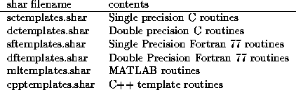
Save the mail message to a file called templates.shar. Edit the
mail header from this file and delete the lines down to and including
<< Cut Here >>. In the directory containing the shar file, type
sh templates.shar
No subdirectory will be created. The unpacked files will stay in the
current directory. Each method is written as a separate subroutine in
its own file, named after the method (e.g., CG.f, BiCGSTAB.f, GMRES.f). The argument parameters are the same
for each, with the exception of the required matrix-vector products
and preconditioner solvers (some require the transpose matrix). Also,
the amount of workspace needed varies. The details are documented in
each routine.
Note that the matrix-vector operations are accomplished using the BLAS
[144] (many manufacturers have assembly coded these
kernels for maximum performance), although a mask file is provided to
link to user defined routines.
The README file gives more details, along with instructions for
a test routine.
Next:
Overview of the
Up:
Templates for the Solution
Previous:
Row Projection Methods
Jack Dongarra
Mon Nov 20 08:52:54 EST 1995
Overview of the BLAS
Next:
Glossary
Up:
Templates for the Solution
Previous:
Obtaining the Software
The BLAS give us a standardized
set of basic codes for performing operations on vectors and matrices.
BLAS take advantage of the Fortran storage structure and the structure
of the mathematical system wherever possible. Additionally, many
computers have the BLAS library optimized to their system. Here we use
five routines:
- SCOPY: copies a vector onto another vector
- SAXPY: adds vector
(multiplied by a scalar) to vector
- SGEMV: general matrix vector product
- STRMV: matrix vector product when the matrix is triangular
- STRSV: solves
 for triangular matrix
The prefix ``S'' denotes single precision. This prefix may be
changed to ``D'', ``C'', or ``Z'', giving
the routine double, complex,
or double complex precision. (Of course, the declarations would also
have to be changed.) It is important to note that putting double precision
into single variables works, but single into double will cause errors.
If we define  a(i,j) and
= x(i), we can see what the
code is doing:
a(i,j) and
= x(i), we can see what the
code is doing:
-
ALPHA = SDOT( N, X, 1, Y, 1 ) computes the inner product of two
vectors
and
, putting the result in scalar  .
.
The corresponding Fortran segment is
ALPHA = 0.0
DO I = 1, N
ALPHA = ALPHA + X(I)*Y(I)
ENDDO
-
CALL SAXPY( N, ALPHA, X, 1, Y ) multiplies a
vector
of length
by the scalar  , then adds the result to
the vector
, putting the result in
.
, then adds the result to
the vector
, putting the result in
.
The corresponding Fortran segment is
DO I = 1, N
Y(I) = ALPHA*X(I) + Y(I)
ENDDO
-
CALL SGEMV( 'N', M, N, ONE, A, LDA, X, 1, ONE, B, 1 )
computes the matrix-vector product plus vector  ,
putting the resulting vector in
,
putting the resulting vector in  .
.
The corresponding Fortran segment:
DO J = 1, N
DO I = 1, M
B(I) = A(I,J)*X(J) + B(I)
ENDDO
ENDDO
This illustrates a feature of the BLAS that often requires close
attention. For example, we will use this routine to compute the residual
vector  , where
  is our current approximation to the
solution
(merely change the fourth argument to -1.0E0). Vector
will be overwritten with the residual vector; thus, if we need it later, we
will first copy it to temporary storage.
is our current approximation to the
solution
(merely change the fourth argument to -1.0E0). Vector
will be overwritten with the residual vector; thus, if we need it later, we
will first copy it to temporary storage.
-
CALL STRMV( 'U', 'N', 'N', N, A, LDA, X, 1 ) computes the
matrix-vector product  , putting the resulting vector in
,
for upper triangular matrix
.
, putting the resulting vector in
,
for upper triangular matrix
.
The corresponding Fortran segment is
DO J = 1, N
TEMP = X(J)
DO I = 1, J
X(I) = X(I) + TEMP*A(I,J)
ENDDO
ENDDO
Note that the parameters in single quotes are for descriptions
such as 'U' for `UPPER TRIANGULAR', 'N' for `No Transpose'. This
feature will be used extensively, resulting in storage savings
(among other advantages).
The variable LDA is critical for addressing the array
correctly. LDA is the leading dimension of the two-dimensional
array A,
that is, LDA is the declared (or allocated) number
of rows of the two-dimensional array
.
Next:
Glossary
Up:
Templates for the Solution
Previous:
Obtaining the Software
Jack Dongarra
Mon Nov 20 08:52:54 EST 1995
Glossary
Next:
Notation
Up:
Templates for the Solution
Previous:
Overview of the
- Adaptive methods
- Iterative methods that collect information
about the coefficient matrix during the iteration process, and use
this to speed up convergence.
- Backward error
- The size of perturbations
 of the
coefficient matrix and
of the
coefficient matrix and  of the right hand side of a linear
system
, such that the computed iterate
is the
solution of
of the right hand side of a linear
system
, such that the computed iterate
is the
solution of  .
.
- Band matrix
- A matrix
for which there are nonnegative
constants
 ,
,  such that
  if
if  or
or  . The
two constants
,
are called the left and right halfbandwidth
respectively.
. The
two constants
,
are called the left and right halfbandwidth
respectively.
- Black box
- A piece of software that can be used without
knowledge of its inner workings; the user supplies the input, and
the output is assumed to be correct.
- BLAS
- Basic Linear Algebra Subprograms; a set of commonly
occurring vector and matrix operations for dense linear algebra.
Optimized (usually assembly coded) implementations of the BLAS exist
for various computers; these will give a higher performance than
implementation in high level programming languages.
- Block factorization
- See: Block matrix operations.
- Block matrix operations
- Matrix operations expressed in terms of
submatrices.
- Breakdown
- The occurrence of a zero divisor in an iterative
method.
- Cholesky decomposition
- Expressing a symmetric matrix
as a
product of a lower triangular matrix
and its transpose
,
that is,
 .
.
- Condition number
- See: Spectral condition number.
- Convergence
- The fact whether or not, or the rate at which, an
iterative method approaches the solution of a linear system.
Convergence can be
- Linear
: some measure of the distance
to the solution decreases by a constant factor in each iteration.
- Superlinear
: the measure of the
error decreases by a growing factor.
- Smooth
: the measure of the error
decreases in all or most iterations, though not necessarily by the
same factor.
- Irregular
: the measure of the error
decreases in some iterations and increases in others. This
observation unfortunately does not imply anything about the ultimate
convergence of the method.
- Stalled
: the measure of the error
stays more or less constant during a number of iterations. As above,
this does not imply anything about the ultimate convergence of the
method.
- Dense matrix
- Matrix for which the number of zero elements is
too small to warrant specialized algorithms to exploit these zeros.
- Diagonally dominant matrix
- See: Matrix properties
- Direct method
- An algorithm that produces the solution to a
system of linear equations in a number of operations that is
determined a priori by the size of the system. In exact arithmetic,
a direct method yields the true solution to the system. See:
Iterative method.
- Distributed memory
- See: Parallel computer.
- Divergence
- An iterative method is said to diverge if it does
not converge in a reasonable number of iterations, or if some
measure of the error grows unacceptably. However, growth of the
error as such is no sign of divergence: a method with irregular
convergence behavior may ultimately converge, even though the error
grows during some iterations.
- Domain decomposition method
- Solution method for linear systems
based on a partitioning of the physical domain of the differential
equation. Domain decomposition methods typically involve (repeated)
independent system solution on the subdomains, and some way of
combining data from the subdomains on the separator part of the
domain.
- Field of values
- Given a matrix
, the field of values is the
set
 . For symmetric matrices this is the range
 .
.
- Fill
- A position that is zero in the original matrix
but not
in an exact factorization of
. In an incomplete factorization,
some fill elements are discarded.
- Forward error
- The difference between a computed iterate and the
true solution of a linear system, measured in some vector norm.
- Halfbandwidth
- See: Band matrix.
- Ill-conditioned system
- A linear system for which the
coefficient matrix has a large condition number. Since in many
applications the condition number is proportional to (some power of)
the number of unknowns, this should be understood as the constant of
proportionality being large.
- IML++
- A mathematical template library in C++
of iterative method for solving linear systems.
- Incomplete factorization
- A factorization obtained by discarding
certain elements during the factorization process (`modified' and
`relaxed' incomplete factorization compensate in some way for
discarded elements). Thus an incomplete
 factorization of a
matrix
will in general satisfy
factorization of a
matrix
will in general satisfy  ; however, one hopes
that the factorization
will be close enough to
to function
as a preconditioner in an iterative method.
; however, one hopes
that the factorization
will be close enough to
to function
as a preconditioner in an iterative method.
- Iterate
- Approximation to the solution of a linear system in any
iteration of an iterative method.
- Iterative method
- An algorithm that produces a sequence of
approximations to the solution of a linear system of equations; the
length of the sequence is not given a priori by the size of the
system. Usually, the longer one iterates, the closer one is able to
get to the true solution. See: Direct method.
- Krylov sequence
- For a given matrix
and vector
, the
sequence of vectors
 , or a finite initial part of
this sequence.
, or a finite initial part of
this sequence.
- Krylov subspace
- The subspace spanned by a Krylov sequence.
- LAPACK
- A mathematical library of linear algebra routine for
dense systems solution and eigenvalue calculations.
- Lower triangular matrix
- Matrix
for which
if
.
 factorization
- A way of writing a matrix
as a product
of a lower triangular matrix
and a unitary matrix
 , that is,
 .
.
-
factorization /
decomposition
- Expressing a matrix
as a product of a lower triangular matrix
and an upper
triangular matrix
, that is,
 .
.
-
-Matrix
- See: Matrix properties.
- Matrix norms
- See: Norms.
- Matrix properties
- We call a square matrix
- Symmetric
- if
 for all
,
.
for all
,
.
- Positive definite
- if it satisfies
 for all nonzero
vectors
.
for all nonzero
vectors
.
- Diagonally dominant
- if
 ; the
excess amount
; the
excess amount 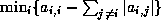 is called
the diagonal dominance of the matrix.
is called
the diagonal dominance of the matrix.
- An
-matrix
- if
 for
for  , and it is
nonsingular with
, and it is
nonsingular with  for all
,
.
for all
,
.
- Message passing
- See: Parallel computer.
- Multigrid method
- Solution method for linear systems based on
restricting and extrapolating solutions between a series of nested
grids.
- Modified incomplete factorization
- See: Incomplete
factorization.
- Mutually consistent norms
- See: Norms.
- Natural ordering
- See: Ordering of unknowns.
- Nonstationary iterative method
- Iterative method that has
iteration-dependent coefficients.
- Normal equations
- For a nonsymmetric or indefinite (but
nonsingular) system of equations
, either of the related
symmetric systems (
 ) and (
 ;
). For complex
,
is replaced with
;
). For complex
,
is replaced with  in the above
expressions.
in the above
expressions.
- Norms
- A function
 is called a vector norm
if
is called a vector norm
if
-
 for all
, and
for all
, and  only if
  .
. -
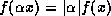 for all
  ,
.
,
.
-
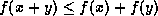 for all
,
.
for all
,
.
The same properties hold for matrix norms. A matrix norm and a
vector norm (both denoted  ) are called a mutually
consistent pair if for all matrices
and vectors
) are called a mutually
consistent pair if for all matrices
and vectors

- Ordering of unknowns
- For linear systems derived from a partial
differential equation, each unknown corresponds to a node in the
discretization mesh. Different orderings of the unknowns correspond
to permutations of the coefficient matrix. The convergence speed of
iterative methods may depend on the ordering used, and often the
parallel efficiency of a method on a parallel computer is strongly
dependent on the ordering used. Some common orderings for
rectangular domains are:
- The natural ordering; this is the consecutive numbering by
rows and columns.
- The red/black ordering; this is the numbering where all nodes
with coordinates
 for which
  is odd are numbered
before those for which
is even.
is odd are numbered
before those for which
is even.
- The ordering by diagonals; this is the ordering where nodes
are grouped in levels for which
is constant. All nodes in
one level are numbered before the nodes in the next level.
For matrices from problems on less regular domains, some common
orderings are:
- The Cuthill-McKee ordering; this starts from one point, then
numbers its neighbors, and continues numbering points that are
neighbors of already numbered points. The Reverse Cuthill-McKee
ordering then reverses the numbering; this may reduce the amount
of fill in a factorization of the matrix.
- The Minimum Degree ordering; this orders the matrix rows by
increasing numbers of nonzeros.
- Parallel computer
- Computer with multiple independent processing
units. If the processors have immediate access to the same memory,
the memory is said to be shared; if processors have private memory
that is not immediately visible to other processors, the memory is
said to be distributed. In that case, processors communicate by
message-passing.
- Pipelining
- See: Vector computer.
- Positive definite matrix
- See: Matrix properties.
- Preconditioner
- An auxiliary matrix in an iterative method that
approximates in some sense the coefficient matrix or its inverse.
The preconditioner, or preconditioning matrix, is applied in every
step of the iterative method.
- Red/black ordering
- See: Ordering of unknowns.
- Reduced system
- Linear system obtained by eliminating certain
variables from another linear system. Although the number of
variables is smaller than for the original system, the matrix of a
reduced system generally has more nonzero entries. If the original
matrix was symmetric and positive definite, then the reduced system
has a smaller condition number.
- Relaxed incomplete factorization
- See: Incomplete factorization.
- Residual
- If an iterative method is employed to solve for
in
a linear system
, then the residual corresponding to a
vector
is
 .
.
- Search direction
- Vector that is used to update an iterate.
- Shared memory
- See: Parallel computer.
- Simultaneous displacements, method of
- Jacobi method.
- Sparse matrix
- Matrix for which the number of zero elements is
large enough that algorithms avoiding operations on zero elements
pay off. Matrices derived from partial differential equations
typically have a number of nonzero elements that is proportional to
the matrix size, while the total number of matrix elements is the
square of the matrix size.
- Spectral condition number
- The product
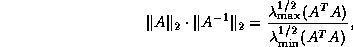
where  and
and  denote the largest and
smallest eigenvalues, respectively. For linear systems derived from
partial differential equations in 2D, the condition number is
proportional to the number of unknowns.
denote the largest and
smallest eigenvalues, respectively. For linear systems derived from
partial differential equations in 2D, the condition number is
proportional to the number of unknowns.
- Spectral radius
- The spectral radius of a matrix
is
.
- Spectrum
- The set of all eigenvalues of a matrix.
- Stationary iterative method
- Iterative method that performs in
each iteration the same operations on the current iteration vectors.
- Stopping criterion
- Since an iterative method computes
successive approximations to the solution of a linear system, a
practical test is needed to determine when to stop the iteration.
Ideally this test would measure the distance of the last iterate to
the true solution, but this is not possible. Instead, various other
metrics are used, typically involving the residual.
- Storage scheme
- The way elements of a matrix are stored in the
memory of a computer. For dense matrices, this can be the decision
to store rows or columns consecutively. For sparse matrices, common
storage schemes avoid storing zero elements; as a result they
involve indices, stored as integer data, that indicate where the
stored elements fit into the global matrix.
- Successive displacements, method of
- Gauss-Seidel method.
- Symmetric matrix
- See: Matrix properties.
- Template
- Description of an algorithm, abstracting away from
implementational details.
- Tune
- Adapt software for a specific application and computing
environment in order to obtain better performance in that case only.
itemize
- Upper triangular matrix
- Matrix
for which
if
 .
.
- Vector computer
- Computer that is able to process consecutive
identical operations (typically additions or multiplications)
several times faster than intermixed operations of different types.
Processing identical operations this way is called `pipelining' the
operations.
- Vector norms
- See: Norms.
Next:
Notation
Up:
Templates for the Solution
Previous:
Overview of the
Jack Dongarra
Mon Nov 20 08:52:54 EST 1995
Notation
Next:
References
Up:
Templates for the Solution
Previous:
Glossary
In this section, we present some of the notation we use
throughout the book.
We have tried to use standard notation that would be found
in any current publication on the subjects covered.
Throughout, we follow several conventions:
- Matrices are denoted by capital letters.
- Vectors are denoted by lowercase letters.
- Lowercase Greek letters usually denote scalars, for instance
- Matrix elements are denoted by doubly indexed lowercase letter,
however
- Matrix subblocks are denoted by doubly indexed uppercase letters.
We define matrix
of dimension  and block dimension
 as follows:
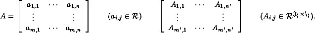
We define vector
of dimension
as follows:
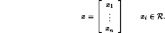
Other notation is as follows:
-
 (or simply
if the size is clear from the
context) denotes the identity matrix.
(or simply
if the size is clear from the
context) denotes the identity matrix.
-
= diag
 denotes that matrix
has elements
denotes that matrix
has elements
 on its diagonal, and zeros everywhere else.
-
 denotes the
th element of vector
during
the
th iteration
denotes the
th element of vector
during
the
th iteration
Jack Dongarra
Mon Nov 20 08:52:54 EST 1995
References
Next:
Index
Up:
Templates for the Solution
Previous:
Notation
References
-
1
-
J. AARDEN AND K.-E. KARLSSON, Preconditioned CG-type methods for
solving the coupled systems of fundamental semiconductor equations, BIT, 29
(1989), pp. 916-937.
-
2
-
L. ADAMS AND H. JORDAN, Is SOR color-blind?, SIAM J. Sci.
Statist. Comput., 7 (1986), pp. 490-506.
-
3
-
E. ANDERSON, ET. AL., LAPACK Users Guide, SIAM, Philadelphia,
1992.
-
4
-
J. APPLEYARD AND I. CHESHIRE, Nested factorization, in Reservoir
Simulation Symposium of the SPE, 1983.
Paper 12264.
-
5
-
M. ARIOLI, J. DEMMEL, AND I. DUFF, Solving sparse linear systems
with sparse backward error, SIAM J. Matrix Anal. Appl., 10 (1989),
pp. 165-190.
-
6
-
W. ARNOLDI, The principle of minimized iterations in the solution of
the matrix eigenvalue problem, Quart. Appl. Math., 9 (1951), pp. 17-29.
-
7
-
S. ASHBY, CHEBYCODE: A Fortran implementation of
Manteuffel's adaptive Chebyshev algorithm, Tech. Rep. UIUCDCS-R-85-1203,
University of Illinois, 1985.
-
8
-
S. ASHBY, T. MANTEUFFEL, AND J. OTTO, A comparison of adaptive
Chebyshev and least squares polynomial preconditioning for Hermitian
positive definite linear systems, SIAM J. Sci. Statist. Comput., 13 (1992),
pp. 1-29.
-
9
-
S. ASHBY, T. MANTEUFFEL, AND P. SAYLOR, Adaptive polynomial
preconditioning for Hermitian indefinite linear systems, BIT, 29 (1989),
pp. 583-609.
-
10
-
S. F. ASHBY, T. A. MANTEUFFEL, AND P. E. SAYLOR, A taxonomy for
conjugate gradient methods, SIAM J. Numer. Anal., 27 (1990), pp. 1542-1568.
-
11
-
C. ASHCRAFT AND R. GRIMES, On vectorizing incomplete factorizations
and SSOR preconditioners, SIAM J. Sci. Statist. Comput., 9 (1988),
pp. 122-151.
-
12
-
O. AXELSSON, Incomplete block matrix factorization preconditioning
methods. The ultimate answer?, J. Comput. Appl. Math., 12& (1985),
pp. 3-18.
-
13
-
height 2pt depth -1.6pt width 23pt, A general incomplete
block-matrix factorization method, Linear Algebra Appl., 74 (1986),
pp. 179-190.
-
14
-
O. AXELSSON AND A. BARKER, Finite element solution of boundary value
problems. Theory and computation, Academic Press, Orlando, Fl., 1984.
-
15
-
O. AXELSSON AND V. EIJKHOUT, Vectorizable preconditioners for
elliptic difference equations in three space dimensions, J. Comput. Appl.
Math., 27 (1989), pp. 299-321.
-
16
-
height 2pt depth -1.6pt width 23pt, The nested recursive
two-level factorization method for nine-point difference matrices, SIAM J.
Sci. Statist. Comput., 12 (1991), pp. 1373-1400.
-
17
-
O. AXELSSON AND I. GUSTAFSSON, Iterative solution for the solution
of the Navier equations of elasticity, Comput. Methods Appl. Mech. Engrg.,
15 (1978), pp. 241-258.
-
18
-
O. AXELSSON AND G. LINDSKOG, On the eigenvalue distribution of a
class of preconditioning matrices, Numer. Math., 48 (1986), pp. 479-498.
-
19
-
height 2pt depth -1.6pt width 23pt, On the rate of
convergence of the preconditioned conjugate gradient method, Numer. Math.,
48 (1986), pp. 499-523.
-
20
-
O. AXELSSON AND N. MUNKSGAARD, Analysis of incomplete factorizations
with fixed storage allocation, in Preconditioning Methods - Theory and
Applications, D. Evans, ed., Gordon and Breach, New York, 1983, pp. 265-293.
-
21
-
O. AXELSSON AND B. POLMAN, On approximate factorization methods for
block-matrices suitable for vector and parallel processors, Linear Algebra
Appl., 77 (1986), pp. 3-26.
-
22
-
O. AXELSSON AND P. VASSILEVSKI, Algebraic multilevel preconditioning
methods, I, Numer. Math., 56 (1989), pp. 157-177.
-
23
-
height 2pt depth -1.6pt width 23pt, Algebraic multilevel
preconditioning methods, II, SIAM J. Numer. Anal., 57 (1990),
pp. 1569-1590.
-
24
-
O. AXELSSON AND P. S. VASSILEVSKI, A black box generalized conjugate
gradient solver with inner iterations and variable-step preconditioning,
SIAM J. Matrix Anal. Appl., 12 (1991), pp. 625-644.
-
25
-
R. BANK, Marching algorithms for elliptic boundary value problems;
II: The variable coefficient case, SIAM J. Numer. Anal., 14 (1977),
pp. 950-970.
-
26
-
R. BANK, T. CHAN, W. COUGHRAN JR., AND R. SMITH, The
Alternate-Block-Factorization procedure for systems of partial
differential equations, BIT, 29 (1989), pp. 938-954.
-
27
-
R. BANK AND D. ROSE, Marching algorithms for elliptic boundary value
problems. I: The constant coefficient case, SIAM J. Numer. Anal., 14
(1977), pp. 792-829.
-
28
-
R. E. BANK AND T. F. CHAN, An analysis of the composite step
Biconjugate gradient method, Numerische Mathematik, 66 (1993),
pp. 295-319.
-
29
-
R. E. BANK AND T. F. CHAN, A composite step bi-conjugate gradient
algorithm for nonsymmetric linear systems, Numer. Alg., (1994), pp. 1-16.
-
30
-
G. BAUDET, Asynchronous iterative methods for multiprocessors, J.
Assoc. Comput. Mach., 25 (1978), pp. 226-244.
-
31
-
R. BEAUWENS, On Axelsson's perturbations, Linear Algebra Appl.,
68 (1985), pp. 221-242.
-
32
-
height 2pt depth -1.6pt width 23pt, Approximate
factorizations with S/P consistently ordered
-factors, BIT, 29
(1989), pp. 658-681.
-
33
-
R. BEAUWENS AND L. QUENON, Existence criteria for partial matrix
factorizations in iterative methods, SIAM J. Numer. Anal., 13 (1976),
pp. 615-643.
-
34
-
A. BJÖRCK AND T. ELFVING, Accelerated projection methods for
computing pseudo-inverse solutions of systems of linear equations, BIT, 19
(1979), pp. 145-163.
-
35
-
D. BRAESS, The contraction number of a multigrid method for solving
the Poisson equation, Numer. Math., 37 (1981), pp. 387-404.
-
36
-
J. H. BRAMBLE, J. E. PASCIAK, AND A. H. SCHATZ, The construction of
preconditioners for elliptic problems by substructuring, I, Mathematics of
Computation, 47 (1986), pp. 103- 134.
-
37
-
J. H. BRAMBLE, J. E. PASCIAK, J. WANG, AND J. XU, Convergence
estimates for product iterative methods with applications to domain
decompositions and multigrid, Math. Comp., 57(195) (1991), pp. 1-21.
-
38
-
R. BRAMLEY AND A. SAMEH, Row projection methods for large
nonsymmetric linear systems, SIAM J. Sci. Statist. Comput., 13 (1992),
pp. 168-193.
-
39
-
C. BREZINSKI AND H. SADOK, Avoiding breakdown in the CGS
algorithm, Numer. Alg., 1 (1991), pp. 199-206.
-
40
-
C. BREZINSKI, M. ZAGLIA, AND H. SADOK, Avoiding breakdown and near
breakdown in Lanczos type algorithms, Numer. Alg., 1 (1991), pp. 261-284.
-
41
-
height 2pt depth -1.6pt width 23pt, A breakdown free
Lanczos type algorithm for solving linear systems, Numer. Math., 63
(1992), pp. 29-38.
-
42
-
W. BRIGGS, A Multigrid Tutorial, SIAM, Philadelphia, 1977.
-
43
-
X.-C. CAI AND O. WIDLUND, Multiplicative Schwarz algorithms for
some nonsymmetric and indefinite problems, SIAM J. Numer. Anal., 30 (1993),
pp. 936-952.
-
44
-
T. CHAN, Fourier analysis of relaxed incomplete factorization
preconditioners, SIAM J. Sci. Statist. Comput., 12 (1991), pp. 668-680.
-
45
-
T. CHAN, L. DE PILLIS, AND H. VAN DER VORST, A transpose-free
squared Lanczos algorithm and application to solving nonsymmetric linear
systems, Tech. Rep. CAM 91-17, UCLA, Dept. of Math., Los Angeles, CA
90024-1555, 1991.
-
46
-
T. CHAN, E. GALLOPOULOS, V. SIMONCINI, T. SZETO, AND C. TONG, A
quasi-minimal residual variant of the Bi-CGSTAB algorithm for nonsymmetric
systems, SIAM J. Sci. Comp., 15(2) (1994), pp. 338-347.
-
47
-
T. CHAN, R. GLOWINSKI, , J. PéRIAUX, AND O. WIDLUND, eds., Domain Decomposition Methods, Philadelphia, 1989, SIAM.
Proceedings of the Second International Symposium on Domain
Decomposition Methods, Los Angeles, CA, January 14 - 16, 1988.
-
48
-
height 2pt depth -1.6pt width 23pt, eds., Domain
Decomposition Methods, Philadelphia, 1990, SIAM.
Proceedings of the Third International Symposium on Domain
Decomposition Methods, Houston, TX, 1989.
-
49
-
height 2pt depth -1.6pt width 23pt, eds., Domain
Decomposition Methods, SIAM, Philadelphia, 1991.
Proceedings of the Fourth International Symposium on Domain
Decomposition Methods, Moscow, USSR, 1990.
-
50
-
T. CHAN AND C.-C. J. KUO, Two-color Fourier analysis of iterative
algorithms for elliptic problems with red/black ordering, SIAM J. Sci.
Statist. Comput., 11 (1990), pp. 767-793.
-
51
-
T. F. CHAN AND T. MATHEW, Domain decomposition algorithms, Acta
Numerica, (1994), pp. 61-144.
-
52
-
T. F. CHAN, T. P. MATHEW, AND J. P. SHAO, Efficient variants of the
vertex space domain decomposition algorithm, SIAM J. Sci. Comput., 15(6)
(1994), pp. 1349-1374.
-
53
-
T. F. CHAN AND J. SHAO, Optimal coarse grid size in domain
decomposition, J. Comput. Math., 12(4) (1994), pp. 291-297.
-
54
-
D. CHAZAN AND W. MIRANKER, Chaotic relaxation, Linear Algebra
Appl., 2 (1969), pp. 199-222.
-
55
-
A. CHRONOPOULOS AND C. GEAR,
-step iterative methods for
symmetric linear systems, J. Comput. Appl. Math., 25 (1989), pp. 153-168.
-
56
-
P. CONCUS AND G. GOLUB, A generalized conjugate gradient method for
nonsymmetric systems of linear equations, in Computer methods in Applied
Sciences and Engineering, Second International Symposium, Dec 15-19, 1975;
Lecture Notes in Economics and Mathematical Systems, Vol. 134, Berlin, New
York, 1976, Springer-Verlag.
-
57
-
P. CONCUS, G. GOLUB, AND G. MEURANT, Block preconditioning for the
conjugate gradient method, SIAM J. Sci. Statist. Comput., 6 (1985),
pp. 220-252.
-
58
-
P. CONCUS, G. GOLUB, AND D. O'LEARY, A generalized conjugate
gradient method for the numerical solution of elliptic partial differential
equations, in Sparse Matrix Computations, J. Bunch and D. Rose, eds.,
Academic Press, New York, 1976, pp. 309-332.
-
59
-
P. CONCUS AND G. H. GOLUB, Use of fast direct methods for the
efficient numerical solution of nonseparable elliptic equations, SIAM J.
Numer. Anal., 10 (1973), pp. 1103-1120.
-
60
-
E. CUTHILL AND J. MCKEE, Reducing the bandwidth of sparse symmetric
matrices, in ACM Proceedings of the 24th National Conference, 1969.
-
61
-
E. D'AZEVEDO, V. EIJKHOUT, AND C. ROMINE, LAPACK working note 56:
Reducing communication costs in the conjugate gradient algorithm on
distributed memory multiprocessor, tech. report, Computer Science
Department, University of Tennessee, Knoxville, TN, 1993.
-
62
-
E. D'AZEVEDO AND C. ROMINE, Reducing communication costs in the
conjugate gradient algorithm on distributed memory multiprocessors, Tech.
Rep. ORNL/TM-12192, Oak Ridge National Lab, Oak Ridge, TN, 1992.
-
63
-
E. DE STURLER, A parallel restructured version of GMRES(m),
Tech. Rep. 91-85, Delft University of Technology, Delft, The Netherlands,
1991.
-
64
-
E. DE STURLER AND D. R. FOKKEMA, Nested Krylov methods and
preserving the orthogonality, Tech. Rep. Preprint 796, Utrecht University,
Utrecht, The Netherlands, 1993.
-
65
-
S. DEMKO, W. MOSS, AND P. SMITH, Decay rates for inverses of band
matrices, Mathematics of Computation, 43 (1984), pp. 491-499.
-
66
-
J. DEMMEL, The condition number of equivalence transformations that
block diagonalize matrix pencils, SIAM J. Numer. Anal., 20 (1983),
pp. 599-610.
-
67
-
J. DEMMEL, M. HEATH, AND H. VAN DER VORST, Parallel numerical linear
algebra, in Acta Numerica, Vol. 2, Cambridge Press, New York, 1993.
-
68
-
S. DOI, On parallelism and convergence of incomplete LU
factorizations, Appl. Numer. Math., 7 (1991), pp. 417-436.
-
69
-
J. DONGARRA, J. DUCROZ, I. DUFF, AND S. HAMMARLING, A set of level
3 Basic Linear Algebra Subprograms, ACM Trans. Math. Soft., 16
(1990), pp. 1-17.
-
70
-
J. DONGARRA, J. DUCROZ, S. HAMMARLING, AND R. HANSON, An extended
set of FORTRAN Basic Linear Algebra Subprograms, ACM Trans. Math.
Soft., 14 (1988), pp. 1-32.
-
71
-
J. DONGARRA, I. DUFF, D. SORENSEN, AND H. VAN DER VORST, Solving
Linear Systems on Vector and Shared Memory Computers, SIAM, Philadelphia,
PA, 1991.
-
72
-
J. DONGARRA AND E. GROSSE, Distribution of mathematical software via
electronic mail, Comm. ACM, 30 (1987), pp. 403-407.
-
73
-
J. DONGARRA, C. MOLER, J. BUNCH, AND G. STEWART, LINPACK Users'
Guide, SIAM, Philadelphia, 1979.
-
74
-
J. DONGARRA AND H. VAN DER VORST, Performance of various computers
using standard sparse linear equations solving techniques, in Computer
Benchmarks, J. Dongarra and W. Gentzsch, eds., Elsevier Science Publishers
B.V., New York, 1993, pp. 177-188.
-
75
-
F. DORR, The direct solution of the discrete Poisson equation on a
rectangle, SIAM Rev., 12 (1970), pp. 248-263.
-
76
-
M. DRYJA AND O. B. WIDLUND, Towards a unified theory of domain
decomposition algorithms for elliptic problems, Tech. Rep. 486, also
Ultracomputer Note 167, Department of Computer Science, Courant Institute,
1989.
-
77
-
D. DUBOIS, A. GREENBAUM, AND G. RODRIGUE, Approximating the inverse
of a matrix for use in iterative algorithms on vector processors, Computing,
22 (1979), pp. 257-268.
-
78
-
I. DUFF, R. GRIMES, AND J. LEWIS, Sparse matrix test problems, ACM
Trans. Math. Soft., 15 (1989), pp. 1-14.
-
79
-
I. DUFF AND G. MEURANT, The effect of ordering on preconditioned
conjugate gradients, BIT, 29 (1989), pp. 635-657.
-
80
-
I. S. DUFF, A. M. ERISMAN, AND J.K.REID, Direct methods for sparse
matrices, Oxford University Press, London, 1986.
-
81
-
T. DUPONT, R. KENDALL, AND H. RACHFORD, An approximate factorization
procedure for solving self-adjoint elliptic difference equations, SIAM J.
Numer. Anal., 5 (1968), pp. 559-573.
-
82
-
E. D'YAKONOV, The method of variable directions in solving systems
of finite difference equations, Soviet Math. Dokl., 2 (1961), pp. 577-580.
TOM 138, 271-274.
-
83
-
L. EHRLICH, An Ad-Hoc SOR method, J. Comput. Phys., 43 (1981),
pp. 31-45.
-
84
-
M. EIERMANN AND R. VARGA, Is the optimal
best for the SOR
iteration method?, Linear Algebra Appl., 182 (1993), pp. 257-277.
-
85
-
V. EIJKHOUT, Analysis of parallel incomplete point factorizations,
Linear Algebra Appl., 154-156 (1991), pp. 723-740.
-
86
-
height 2pt depth -1.6pt width 23pt, Beware of
unperturbed modified incomplete point factorizations, in Proceedings of the
IMACS International Symposium on Iterative Methods in Linear Algebra,
Brussels, Belgium, R. Beauwens and P. de Groen, eds., 1992.
-
87
-
height 2pt depth -1.6pt width 23pt, LAPACK working
note 50: Distributed sparse data structures for linear algebra operations,
Tech. Rep. CS 92-169, Computer Science Department, University of Tennessee,
Knoxville, TN, 1992.
-
88
-
height 2pt depth -1.6pt width 23pt, LAPACK working
note 51: Qualitative properties of the conjugate gradient and Lanczos
methods in a matrix framework, Tech. Rep. CS 92-170, Computer Science
Department, University of Tennessee, Knoxville, TN, 1992.
-
89
-
V. EIJKHOUT AND B. POLMAN, Decay rates of inverses of banded
-matrices that are near to Toeplitz matrices, Linear Algebra Appl.,
109 (1988), pp. 247-277.
-
90
-
V. EIJKHOUT AND P. VASSILEVSKI, Positive definiteness aspects of
vectorizable preconditioners, Parallel Computing, 10 (1989), pp. 93-100.
-
91
-
S. EISENSTAT, Efficient implementation of a class of preconditioned
conjugate gradient methods, SIAM J. Sci. Statist. Comput., 2 (1981),
pp. 1-4.
-
92
-
R. ELKIN, Convergence theorems for Gauss-Seidel and other
minimization algorithms, Tech. Rep. 68-59, Computer Science Center,
University of Maryland, College Park, MD, Jan. 1968.
-
93
-
H. ELMAN, Approximate Schur complement preconditioners on serial
and parallel computers, SIAM J. Sci. Statist. Comput., 10 (1989),
pp. 581-605.
-
94
-
H. ELMAN AND M. SCHULTZ, Preconditioning by fast direct methods for
non self-adjoint nonseparable elliptic equations, SIAM J. Numer. Anal., 23
(1986), pp. 44-57.
-
95
-
L. ELSNER, A note on optimal block-scaling of matrices, Numer.
Math., 44 (1984), pp. 127-128.
-
96
-
V. FABER AND T. MANTEUFFEL, Necessary and sufficient conditions for
the existence of a conjugate gradient method, SIAM J. Numer. Anal., 21
(1984), pp. 315-339.
-
97
-
G. FAIRWEATHER, A. GOURLAY, AND A. MITCHELL, Some high accuracy
difference schemes with a splitting operator for equations of parabolic and
elliptic type, Numer. Math., 10 (1967), pp. 56-66.
-
98
-
R. FLETCHER, Conjugate gradient methods for indefinite systems, in
Numerical Analysis Dundee 1975, G. Watson, ed., Berlin, New York, 1976,
Springer Verlag, pp. 73-89.
-
99
-
G. FORSYTHE AND E. STRAUSS, On best conditioned matrices, Proc.
Amer. Math. Soc., 6 (1955), pp. 340-345.
-
100
-
R. FREUND, Conjugate gradient-type methods for linear systems with
complex symmetric coefficient matrices, SIAM J. Sci. Statist. Comput., 13
(1992), pp. 425-448.
-
101
-
R. FREUND, M. GUTKNECHT, AND N. NACHTIGAL, An implementation of the
look-ahead Lanczos algorithm for non-Hermitian matrices, SIAM J. Sci.
Comput., 14 (1993), pp. 137-158.
-
102
-
R. FREUND AND N. NACHTIGAL, QMR: A quasi-minimal residual method
for non-Hermitian linear systems, Numer. Math., 60 (1991), pp. 315-339.
-
103
-
height 2pt depth -1.6pt width 23pt, An implementation of
the QMR method based on coupled two-term recurrences, SIAM J. Sci.
Statist. Comput., 15 (1994), pp. 313-337.
-
104
-
R. FREUND AND T. SZETO, A quasi-minimal residual squared algorithm
for non-Hermitian linear systems, Tech. Rep. CAM Report 92-19, UCLA Dept.
of Math., 1992.
-
105
-
R. W. FREUND, A transpose-free quasi-minimum residual algorithm for
non-Hermitian linear systems, SIAM J. Sci. Comput., 14 (1993),
pp. 470-482.
-
106
-
R. W. FREUND, G. H. GOLUB, AND N. M. NACHTIGAL, Iterative solution
of linear systems, Acta Numerica, (1992), pp. 57-100.
-
107
-
R. GLOWINSKI, G. H. GOLUB, G. A. MEURANT, AND J. PéRIAUX, eds., Domain Decomposition Methods for Partial Differential Equations, SIAM,
Philadelphia, 1988.
Proceedings of the First International Symposium on Domain
Decomposition Methods for Partial Differential Equations, Paris,
France, January 1987.
-
108
-
G. GOLUB AND D. O'LEARY, Some history of the conjugate gradient and
Lanczos methods, SIAM Rev., 31 (1989), pp. 50-102.
-
109
-
G. GOLUB AND C. VAN LOAN, Matrix Computations, second
edition, The Johns Hopkins University Press, Baltimore, 1989.
-
110
-
A. GREENBAUM AND Z. STRAKOS, Predicting the behavior of finite
precision Lanczos and conjugate gradient computations, SIAM J. Mat.
Anal. Appl., 13 (1992), pp. 121-137.
-
111
-
W. D. GROPP AND D. E. KEYES, Domain decomposition with local mesh
refinement, SIAM J. Sci. Statist. Comput., 13 (1992), pp. 967-993.
-
112
-
I. GUSTAFSSON, A class of first-order factorization methods, BIT,
18 (1978), pp. 142-156.
-
113
-
M. H. GUTKNECHT, The unsymmetric Lanczos algorithms and their
relations to Páde approximation, continued fractions and the QD
algorithm, in Proceedings of the Copper Mountain Conference on Iterative
Methods, 1990.
-
114
-
height 2pt depth -1.6pt width 23pt, A completed theory
of the unsymmetric Lanczos process and related algorithms, part I, SIAM
J. Matrix Anal. Appl., 13 (1992), pp. 594-639.
-
115
-
height 2pt depth -1.6pt width 23pt, Variants of
Bi-CGSTAB for matrices with complex spectrum, SIAM J. Sci. Comp., 14
(1993), pp. 1020-1033.
-
116
-
height 2pt depth -1.6pt width 23pt, A completed theory
of the unsymmetric Lanczos process and related algorithms, part II, SIAM
J. Matrix Anal. Appl., 15 (1994), pp. 15-58.
-
117
-
W. HACKBUSCH, Multi-Grid Methods and Applications, Springer-Verlag,
Berlin, New York, 1985.
-
118
-
height 2pt depth -1.6pt width 23pt, Iterative Lösung
großer schwachbesetzter Gleichungssysteme, Teubner, Stuttgart, 1991.
-
119
-
A. HADJIDIMOS, On some high accuracy difference schemes for solving
elliptic equations, Numer. Math., 13 (1969), pp. 396-403.
-
120
-
L. HAGEMAN AND D. YOUNG, Applied Iterative Methods, Academic Press,
New York, 1981.
-
121
-
W. HAGER, Condition estimators, SIAM J. Sci. Statist. Comput., 5
(1984), pp. 311-316.
-
122
-
M. HESTENES AND E. STIEFEL, Methods of conjugate gradients for
solving linear systems, J. Res. Nat. Bur. Stand., 49 (1952), pp. 409-436.
-
123
-
M. R. HESTENES, Conjugacy and gradients, in A History of Scientific
Computing, Addison-Wesley, Reading, MA, 1990, pp. 167-179.
-
124
-
N. HIGHAM, Experience with a matrix norm estimator, SIAM J. Sci.
Statist. Comput., 11 (1990), pp. 804-809.
-
125
-
K. JEA AND D. YOUNG, Generalized conjugate-gradient acceleration of
nonsym- metrizable iterative methods, Linear Algebra Appl., 34 (1980),
pp. 159-194.
-
126
-
O. JOHNSON, C. MICCHELLI, AND G. PAUL, Polynomial preconditioning
for conjugate gradient calculation, SIAM J. Numer. Anal., 20 (1983),
pp. 362-376.
-
127
-
M. JONES AND P. PLASSMANN, Parallel solution of unstructed, sparse
systems of linear equations, in Proceedings of the Sixth SIAM conference on
Parallel Processing for Scientific Computing, R. Sincovec, D. Keyes,
M. Leuze, L. Petzold, and D. Reed, eds., SIAM, Philadelphia, pp. 471-475.
-
128
-
height 2pt depth -1.6pt width 23pt, A parallel graph
coloring heuristic, SIAM J. Sci. Statist. Comput., 14 (1993), pp. 654-669.
-
129
-
W. JOUBERT, Lanczos methods for the solution of nonsymmetric systems
of linear equations, SIAM J. Matrix Anal. Appl., 13 (1992), pp. 926-943.
-
130
-
W. KAHAN, Gauss-Seidel methods of solving large systems of linear
equations, PhD thesis, University of Toronto, 1958.
-
131
-
S. KANIEL, Estimates for some computational techniques in linear
algebra, Mathematics of Computation, 20 (1966), pp. 369-378.
-
132
-
D. KERSHAW, The incomplete Cholesky-conjugate gradient method for
the iterative solution of systems of linear equations, J. Comput. Phys., 26
(1978), pp. 43-65.
-
133
-
R. KETTLER, Analysis and comparison of relaxation schemes in robust
multigrid and preconditioned conjugate gradient methods, in Multigrid
Methods, Lecture Notes in Mathematics 960, W. Hackbusch and U. Trottenberg,
eds., Springer-Verlag, Berlin, New York, 1982, pp. 502-534.
-
134
-
height 2pt depth -1.6pt width 23pt, Linear multigrid
methods in numerical reservoir simulation, PhD thesis, Delft University of
Technology, Delft, The Netherlands, 1987.
-
135
-
D. E. KEYES, T. F. CHAN, G. MEURANT, J. S. SCROGGS, AND R. G. VOIGT,
eds., Domain Decomposition Methods For Partial Differential Equations,
SIAM, Philadelphia, 1992.
Proceedings of the Fifth International Symposium on Domain
Decomposition Methods, Norfolk, VA, 1991.
-
136
-
D. E. KEYES AND W. D. GROPP, A comparison of domain decomposition
techniques for elliptic partial differential equations and their parallel
implementation, SIAM J. Sci. Statist. Comput., 8 (1987), pp. s166 - s202.
-
137
-
height 2pt depth -1.6pt width 23pt, Domain decomposition
for nonsymmetric systems of equations: Examples from computational fluid
dynamics, in Domain Decomposition Methods, proceedings of the Second
Internation Symposium, Los Angeles, California, January 14-16, 1988, T. F.
Chan, R. Glowinski, J. Periaux, and O. B. Widlund, eds., Philadelphia, 1989,
SIAM, pp. 373-384.
-
138
-
height 2pt depth -1.6pt width 23pt, Domain decomposition
techniques for the parallel solution of nonsymmetric systems of elliptic
boundary value problems, Applied Num. Math., 6 (1989/1990), pp. 281-301.
-
139
-
S. K. KIM AND A. T. CHRONOPOULOS, A class of Lanczos-like
algorithms implemented on parallel computers, Parallel Comput., 17 (1991),
pp. 763-778.
-
140
-
D. R. KINCAID, J. R. RESPESS, D. M. YOUNG, AND R. G. GRIMES, ITPACK 2C: A Fortran package for solving large sparse linear systems
by adaptive accelerated iterative methods, ACM Trans. Math. Soft., 8 (1982),
pp. 302-322.
Algorithm 586.
-
141
-
L. Y. KOLOTILINA AND A. Y. YEREMIN, On a family of two-level
preconditionings of the incomlete block factorization type, Sov. J. Numer.
Anal. Math. Modelling, (1986), pp. 293-320.
-
142
-
C. LANCZOS, An iteration method for the solution of the eigenvalue
problem of linear differential and integral operators, J. Res. Nat. Bur.
Stand., 45 (1950), pp. 255-282.
-
143
-
height 2pt depth -1.6pt width 23pt, Solution of systems
of linear equations by minimized iterations, J. Res. Nat. Bur. Stand., 49
(1952), pp. 33-53.
-
144
-
C. LAWSON, R. HANSON, D. KINCAID, AND F. KROGH, Basic Linear
Algebra Subprograms for FORTRAN usage, ACM Trans. Math. Soft., 5
(1979), pp. 308-325.
-
145
-
J. MAITRE AND F. MUSY, The contraction number of a class of
two-level methods; an exact evaluation for some finite element subspaces and
model problems, in Multigrid methods, Proceedings, Köln-Porz, 1981,
W. Hackbusch and U. Trottenberg, eds., vol. 960 of Lecture Notes in
Mathematics, 1982, pp. 535-544.
-
146
-
T. MANTEUFFEL, The Tchebychev iteration for nonsymmetric linear
systems, Numer. Math., 28 (1977), pp. 307-327.
-
147
-
height 2pt depth -1.6pt width 23pt, An incomplete
factorization technique for positive definite linear systems, Mathematics of
Computation, 34 (1980), pp. 473-497.
-
148
-
S. MCCORMICK, Multilevel Adaptive Methods for Partial Differential
Equations, SIAM, Philadelphia, 1989.
-
149
-
S. MCCORMICK AND J. THOMAS, The Fast Adaptive Composite grid
(FAC) method for elliptic equations, Mathematics of Computation, 46
(1986), pp. 439-456.
-
150
-
U. MEIER AND A. SAMEH, The behavior of conjugate gradient algorithms
on a multivector processor with a hierarchical memory, J. Comput. Appl.
Math., 24 (1988), pp. 13-32.
-
151
-
U. MEIER-YANG, Preconditioned conjugate gradient-like methods for
nonsymmetric linear systems, tech. rep., CSRD, University of Illinois,
Urbana, IL, April 1992.
-
152
-
J. MEIJERINK AND H. VAN DER VORST, An iterative solution method for
linear systems of which the coefficient matrix is a symmetric
-matrix,
Mathematics of Computation, 31 (1977), pp. 148-162.
-
153
-
height 2pt depth -1.6pt width 23pt, Guidelines for the
usage of incomplete decompositions in solving sets of linear equations as
they occur in practical problems, J. Comput. Phys., 44 (1981), pp. 134-155.
-
154
-
R. MELHEM, Toward efficient implementation of preconditioned
conjugate gradient methods on vector supercomputers, Internat. J.
Supercomput. Appls., 1 (1987), pp. 77-98.
-
155
-
G. MEURANT, The block preconditioned conjugate gradient method on
vector computers, BIT, 24 (1984), pp. 623-633.
-
156
-
height 2pt depth -1.6pt width 23pt, Multitasking the
conjugate gradient method on the CRAY X-MP/48, Parallel Comput., 5
(1987), pp. 267-280.
-
157
-
N. MUNKSGAARD, Solving sparse symmetric sets of linear equations by
preconditioned conjugate gradients, ACM Trans. Math. Software, 6 (1980),
pp. 206-219.
-
158
-
N. NACHTIGAL, S. REDDY, AND L. TREFETHEN, How fast are nonsymmetric
matrix iterations?, SIAM J. Matrix Anal. Appl., 13 (1992), pp. 778-795.
-
159
-
N. NACHTIGAL, L. REICHEL, AND L. TREFETHEN, A hybrid GMRES
algorithm for nonsymmetric matrix iterations, SIAM J. Sci. Statist. Comput.,
13 (1992), pp. 796-825.
-
160
-
N. M. NACHTIGAL, A Look-Ahead Variant of the Lanczos Algorithm and
its Application to the Quasi-Minimal Residual Methods for Non-Hermitian
Linear Systems, PhD thesis, MIT, Cambridge, MA, 1991.
-
161
-
Y. NOTAY, Solving positive (semi)definite linear systems by
preconditioned iterative methods, in Preconditioned Conjugate Gradient
Methods, O. Axelsson and L. Kolotilina, eds., vol. 1457 of Lecture Notes in
Mathematics, Nijmegen, 1989, pp. 105-125.
-
162
-
height 2pt depth -1.6pt width 23pt, On the robustness of
modified incomplete factorization methods, Internat. J. Comput. Math., 40
(1992), pp. 121-141.
-
163
-
D. O'LEARY, The block conjugate gradient algorithm and related
methods, Linear Algebra Appl., 29 (1980), pp. 293-322.
-
164
-
height 2pt depth -1.6pt width 23pt, Ordering schemes for
parallel processing of certain mesh problems, SIAM J. Sci. Statist. Comput.,
5 (1984), pp. 620-632.
-
165
-
T. C. OPPE, W. D. JOUBERT, AND D. R. KINCAID, NSPCG user's guide,
version 1.0: A package for solving large sparse linear systems by various
iterative methods, Tech. Rep. CNA-216, Center for Numerical Analysis,
University of Texas at Austin, Austin, TX, April 1988.
-
166
-
J. M. ORTEGA, Introduction to Parallel and Vector Solution of Linear
Systems, Plenum Press, New York and London, 1988.
-
167
-
C. PAIGE, B. PARLETT, AND H. VAN DER VORST, Approximate solutions
and eigenvalue bounds from Krylov subspaces, Numer. Lin. Alg. Appls., 29
(1995), pp. 115-134.
-
168
-
C. PAIGE AND M. SAUNDERS, Solution of sparse indefinite systems of
linear equations, SIAM J. Numer. Anal., 12 (1975), pp. 617-629.
-
169
-
C. C. PAIGE AND M. A. SAUNDERS, LSQR: An algorithm for sparse
linear equations and sparse least squares, ACM Trans. Math. Soft., 8 (1982),
pp. 43-71.
-
170
-
G. PAOLINI AND G. RADICATI DI BROZOLO, Data structures to
vectorize CG algorithms for general sparsity patterns, BIT, 29 (1989),
pp. 703-718.
-
171
-
B. PARLETT, The symmetric eigenvalue problem, Prentice-Hall,
London, 1980.
-
172
-
B. N. PARLETT, D. R. TAYLOR, AND Z. A. LIU, A look-ahead Lanczos
algorithm for unsymmetric matrices, Mathematics of Computation, 44 (1985),
pp. 105-124.
-
173
-
D. PEACEMAN AND J. H.H. RACHFORD, The numerical solution of
parabolic and elliptic differential equations, J. Soc. Indust. Appl. Math.,
3 (1955), pp. 28-41.
-
174
-
C. POMMERELL, Solution of Large Unsymmetric Systems of Linear
Equations, vol. 17 of Series in Micro-electronics, volume 17, Hartung-Gorre
Verlag, Konstanz, 1992.
-
175
-
height 2pt depth -1.6pt width 23pt, Solution of large
unsymmetric systems of linear equations, PhD thesis, Swiss Federal Institute
of Technology, Zürich, Switzerland, 1992.
-
176
-
E. POOLE AND J. ORTEGA, Multicolor ICCG methods for vector
computers, Tech. Rep. RM 86-06, Department of Applied Mathematics,
University of Virginia, Charlottesville, VA, 1986.
-
177
-
A. QUARTERONI, J. PERIAUX, Y. KUZNETSOV, AND O. WIDLUND, eds., Domain Decomposition Methods in Science and Engineering,, vol. Contemporary
Mathematics 157, Providence, RI, 1994, AMS.
Proceedings of the Sixth International Symposium on Domain
Decomposition Methods, June 15-19, 1992, Como, Italy,.
-
178
-
G. RADICATI DI BROZOLO AND Y. ROBERT, Vector and parallel
CG-like algorithms for sparse non-symmetric systems, Tech. Rep. 681-M,
IMAG/TIM3, Grenoble, France, 1987.
-
179
-
J. REID, On the method of conjugate gradients for the solution of
large sparse systems of linear equations, in Large Sparse Sets of Linear
Equations, J. Reid, ed., Academic Press, London, 1971, pp. 231-254.
-
180
-
G. RODRIGUE AND D. WOLITZER, Preconditioning by incomplete block
cyclic reduction, Mathematics of Computation, 42 (1984), pp. 549-565.
-
181
-
Y. SAAD, The Lanczos biorthogonalization algorithm and other
oblique projection methods for solving large unsymmetric systems, SIAM J.
Numer. Anal., 19 (1982), pp. 485-506.
-
182
-
height 2pt depth -1.6pt width 23pt, Practical use of
some Krylov subspace methods for solving indefinite and nonsymmetric linear
systems, SIAM J. Sci. Statist. Comput., 5 (1984), pp. 203-228.
-
183
-
height 2pt depth -1.6pt width 23pt, Practical use of
polynomial preconditionings for the conjugate gradient method, SIAM J. Sci.
Statist. Comput., 6 (1985), pp. 865-881.
-
184
-
height 2pt depth -1.6pt width 23pt, Preconditioning
techniques for indefinite and nonsymmetric linear systems, J. Comput. Appl.
Math., 24 (1988), pp. 89-105.
-
185
-
height 2pt depth -1.6pt width 23pt, Krylov subspace
methods on supercomputers, SIAM J. Sci. Statist. Comput., 10 (1989),
pp. 1200-1232.
-
186
-
height 2pt depth -1.6pt width 23pt, SPARSKIT: A basic
tool kit for sparse matrix computation, Tech. Rep. CSRD TR 1029, CSRD,
University of Illinois, Urbana, IL, 1990.
-
187
-
height 2pt depth -1.6pt width 23pt, A flexible
inner-outer preconditioned GMRES algorithm, SIAM J. Sci. Comput., 14
(1993), pp. 461-469.
-
188
-
Y. SAAD AND M. SCHULTZ, Conjugate gradient-like algorithms for
solving nonsymmetric linear systems, Mathematics of Computation, 44 (1985),
pp. 417-424.
-
189
-
height 2pt depth -1.6pt width 23pt, GMRES: A
generalized minimal residual algorithm for solving nonsymmetric linear
systems, SIAM J. Sci. Statist. Comput., 7 (1986), pp. 856-869.
-
190
-
G. L. G. SLEIJPEN AND D. R. FOKKEMA, Bi-CGSTAB(
 ) for linear
equations involving unsymmetric matrices with complex spectrum, Elec. Trans.
Numer. Anal., 1 (1993), pp. 11-32.
) for linear
equations involving unsymmetric matrices with complex spectrum, Elec. Trans.
Numer. Anal., 1 (1993), pp. 11-32.
-
191
-
B. F. SMITH, Domain decomposition algorithms for partial
differential equations of linear elasticity, Tech. Rep. 517, Department of
Computer Science, Courant Institute, 1990.
-
192
-
P. SONNEVELD, CGS, a fast Lanczos-type solver for nonsymmetric
linear systems, SIAM J. Sci. Statist. Comput., 10 (1989), pp. 36-52.
-
193
-
R. SOUTHWELL, Relaxation Methods in Theoretical Physics, Clarendon
Press, Oxford, 1946.
-
194
-
H. STONE, Iterative solution of implicit approximations of
multidimensional partial differential equations, SIAM J. Numer. Anal., 5
(1968), pp. 530-558.
-
195
-
P. SWARZTRAUBER, The methods of cyclic reduction, Fourier analysis
and the FACR algorithm for the discrete solution of Poisson's equation on
a rectangle, SIAM Rev., 19 (1977), pp. 490-501.
-
196
-
P. L. TALLEC, Domain decomposition methods in computational
mechanics, Computational Mechanics Advances, 1994.
-
197
-
C. TONG, A comparative study of preconditioned Lanczos methods for
nonsymmetric linear systems, Tech. Rep. SAND91-8240, Sandia Nat. Lab.,
Livermore, CA, 1992.
-
198
-
A. VAN DER SLUIS, Condition numbers and equilibration of matrices,
Numer. Math., 14 (1969), pp. 14-23.
-
199
-
A. VAN DER SLUIS AND H. VAN DER VORST, The rate of convergence of
conjugate gradients, Numer. Math., 48 (1986), pp. 543-560.
-
200
-
H. VAN DER VORST, Iterative solution methods for certain sparse
linear systems with a non-symmetric matrix arising from PDE-problems, J.
Comput. Phys., 44 (1981), pp. 1-19.
-
201
-
height 2pt depth -1.6pt width 23pt, A vectorizable
variant of some ICCG methods, SIAM J. Sci. Statist. Comput., 3 (1982),
pp. 350-356.
-
202
-
height 2pt depth -1.6pt width 23pt, Large tridiagonal
and block tridiagonal linear systems on vector and parallel computers,
Parallel Comput., 5 (1987), pp. 45-54.
-
203
-
height 2pt depth -1.6pt width 23pt, (M)ICCG for 2D
problems on vector computers, in Supercomputing, A.Lichnewsky and C.Saguez,
eds., North-Holland, 1988.
-
204
-
height 2pt depth -1.6pt width 23pt, High performance
preconditioning, SIAM J. Sci. Statist. Comput., 10 (1989), pp. 1174-1185.
-
205
-
height 2pt depth -1.6pt width 23pt, ICCG and related
methods for 3D problems on vector computers, Computer Physics
Communications, 53 (1989), pp. 223-235.
-
206
-
height 2pt depth -1.6pt width 23pt, The convergence
behavior of preconditioned CG and CG-S in the presence of rounding
errors, in Preconditioned Conjugate Gradient Methods, O. Axelsson and L. Y.
Kolotilina, eds., vol. 1457 of Lecture Notes in Mathematics, Berlin, New
York, 1990, Springer-Verlag.
-
207
-
height 2pt depth -1.6pt width 23pt, Bi-CGSTAB: A
fast and smoothly converging variant of Bi-CG for the solution of
nonsymmetric linear systems, SIAM J. Sci. Statist. Comput., 13 (1992),
pp. 631-644.
-
208
-
H. VAN DER VORST AND J. MELISSEN, A Petrov-Galerkin type method
for solving
where
is symmetric complex, IEEE Trans.
Magnetics, 26 (1990), pp. 706-708.
-
209
-
H. VAN DER VORST AND C. VUIK, GMRESR: A family of nested GMRES
methods, Numer. Lin. Alg. Applic., 1 (1994), pp. 369-386.
-
210
-
J. VAN ROSENDALE, Minimizing inner product data dependencies in
conjugate gradient iteration, Tech. Rep. 172178, ICASE, NASA Langley
Research Center, 1983.
-
211
-
R. VARGA, Matrix Iterative Analysis, Prentice-Hall Inc., Englewood
Cliffs, NJ, 1962.
-
212
-
P. VASSILEVSKI, Preconditioning nonsymmetric and indefinite finite
element matrices, J. Numer. Alg. Appl., 1 (1992), pp. 59-76.
-
213
-
V. VOEVODIN, The problem of non-self-adjoint generalization of the
conjugate gradient method is closed, U.S.S.R. Comput. Maths. and Math.
Phys., 23 (1983), pp. 143-144.
-
214
-
H. F. WALKER, Implementation of the GMRES method using
Householder transformations, SIAM J. Sci. Statist. Comput., 9 (1988),
pp. 152-163.
-
215
-
P. WESSELING, An Introduction to Multigrid Methods, Wiley,
Chichester, 1991.
-
216
-
O. WIDLUND, A Lanczos method for a class of non-symmetric systems
of linear equations, SIAM J. Numer. Anal., 15 (1978), pp. 801-812.
-
217
-
D. YOUNG, Iterative solution of large linear systems, Academic
Press, New York, 1971.
-
218
-
H. YSERENTANT, On the multilevel splitting of finite element
spaces, Numer. Math., 49 (1986), pp. 379-412.
=0pt plus 40pt
Jack Dongarra
Mon Nov 20 08:52:54 EST 1995
Index
Next:
About this document
Up:
Templates for the Solution
Previous:
References
- ad hoc SOR method
- seemethod, ad hoc SOR
- asynchronous method
- seemethod, asynchronous
- Bi-CGSTAB method
- seemethod, Bi-CGSTAB
- Bi-Conjugate Gradient Stabilized method
- seemethod, Bi-CGSTAB
- bi-orthogonality
- in BiCG
-
BiConjugate Gradient (BiCG)
- in QMR
-
Quasi-Minimal Residual (QMR)
- BiCG method
- seemethod, BiCG
- BiConjugate Gradient method
- seemethod, BiCG
- BLAS
-
Why Use Templates?
- BLAS
-
CRS-based Factorization Solve
- block methods
- (, )
- breakdown
- avoiding by look-ahead
-
Convergence
- in Bi-CGSTAB
-
Convergence
- in BiCG
-
Convergence,
Convergence,
Convergence,
Quasi-Minimal Residual (QMR)
- in BiCG
-
Convergence,
Convergence,
Convergence,
Quasi-Minimal Residual (QMR)
- in BiCG
-
Convergence,
Convergence,
Convergence,
Quasi-Minimal Residual (QMR)
- in BiCG
-
Convergence,
Convergence,
Convergence,
Quasi-Minimal Residual (QMR)
- in CG for indefinite systems
-
MINRES and SYMMLQ
- CG method
- seemethod, CG
- CGNE method
- seemethod, CGNE
- CGNR method
- seemethod, CGNR
- CGS method
- seemethod, CGS
- chaotic method
- seemethod, asynchronous
- Chebyshev iteration
- seemethod, Chebyshev iteration
- codes
- C++
-
Why Use Templates?
- FORTRAN
-
Why Use Templates?
- MATLAB
-
Why Use Templates?
- complex systems
- (, )
- Conjugate Gradient method
- seemethod, CG
- Conjugate Gradient Squared method
- seemethod, CGS
- convergence
- irregular
-
Glossary
- irregular
-
Glossary
- irregular
-
Glossary
- irregular
-
Glossary
- irregular
-
Glossary
- irregular
-
Glossary
- linear
-
Glossary
- of Bi-CGSTAB
- (, )
- of Bi-CGSTAB
- (, )
- of BiCG
- (, )
- of BiCG
- (, )
- of CG
- (, )
- of CG
- (, )
- of CGNR and CGNE
-
Theory
- of CGS
- (, )
- of CGS
- (, )
- of Chebyshev iteration
- (, )
- of Chebyshev iteration
- (, )
- of Gauss-Seidel
-
The Gauss-Seidel Method
- of Jacobi
- (, )
- of Jacobi
- (, )
- of MINRES
-
MINRES and SYMMLQ
- of QMR
- (, )
- of QMR
- (, )
- of SSOR
-
The Symmetric Successive
- smooth
-
Glossary
- smooth
-
Glossary
- stalled
-
Glossary
- stalled
-
Glossary
- stalled
-
Glossary
- superlinear
-
Glossary
- superlinear
-
Glossary
- superlinear
-
Glossary
- superlinear
-
Glossary
- data structures
- (, )
- diffusion
- artificial
-
Modified incomplete factorizations
- domain decomposition
- multiplicative Schwarz
- (, )
- multiplicative Schwarz
- (, )
- non-overlapping subdomains
- (, )
- non-overlapping subdomains
- (, )
- overlapping subdomains
- (, )
- overlapping subdomains
- (, )
- Schur complement
-
Domain Decomposition Methods
- Schwarz
-
Domain Decomposition Methods
- fill-in strategies
- seepreconditioners, point incomplete"factorizations
- FORTRAN codes
- seecodes, FORTRAN
- Gauss-Seidel method
- seemethod, Gauss-Seidel
- Generalized Minimal Residual method
- seemethod, GMRES
- GMRES method
- seemethod, GMRES
- ill-conditioned systems
- using GMRES on
-
Implementation
- implementation
- of Bi-CGSTAB
- (, )
- of Bi-CGSTAB
- (, )
- of BiCG
- (, )
- of BiCG
- (, )
- of CG
- (, )
- of CG
- (, )
- of CGS
- (, )
- of CGS
- (, )
- of Chebyshev iteration
- (, )
- of Chebyshev iteration
- (, )
- of GMRES
- (, )
- of GMRES
- (, )
- of QMR
- (, )
- of QMR
- (, )
- IMSL
-
Introduction
- inner products
- as bottlenecks
-
Implementation,
Chebyshev Iteration,
Comparison with other
- as bottlenecks
-
Implementation,
Chebyshev Iteration,
Comparison with other
- as bottlenecks
-
Implementation,
Chebyshev Iteration,
Comparison with other
- avoiding with Chebyshev
-
Chebyshev Iteration,
Comparison with other ,
Comparison with other ,
Implementation
- avoiding with Chebyshev
-
Chebyshev Iteration,
Comparison with other ,
Comparison with other ,
Implementation
- avoiding with Chebyshev
-
Chebyshev Iteration,
Comparison with other ,
Comparison with other ,
Implementation
- avoiding with Chebyshev
-
Chebyshev Iteration,
Comparison with other ,
Comparison with other ,
Implementation
- irregular convergence
- seeconvergence, irregular
- ITPACK
-
Choosing the Value
- Jacobi method
- seemethod, Jacobi
- Krylov subspace
-
Theory
- Lanczos
- and CG
-
Theory, (, )
- and CG
-
Theory, (, )
- and CG
-
Theory, (, )
- LAPACK
-
Introduction
- linear convergence
- seeconvergence, linear
- LINPACK
-
Introduction
- MATLAB codes
- seecodes, MATLAB
- method
- ad hoc SOR
-
Notes and References
- adaptive Chebyshev
-
Chebyshev Iteration,
Comparison with other
- adaptive Chebyshev
-
Chebyshev Iteration,
Comparison with other
- asynchronous
-
Notes and References
- Bi-CGSTAB
-
What Methods Are ,
Overview of the , (ii, )
- Bi-CGSTAB
-
What Methods Are ,
Overview of the , (ii, )
- Bi-CGSTAB
-
What Methods Are ,
Overview of the , (ii, )
- Bi-CGSTAB
-
What Methods Are ,
Overview of the , (ii, )
- Bi-CGSTAB2
-
Convergence
- BiCG
-
What Methods Are ,
Overview of the , (ii, )
- BiCG
-
What Methods Are ,
Overview of the , (ii, )
- BiCG
-
What Methods Are ,
Overview of the , (ii, )
- BiCG
-
What Methods Are ,
Overview of the , (ii, )
- CG
-
What Methods Are ,
Overview of the , (ii, )
- CG
-
What Methods Are ,
Overview of the , (ii, )
- CG
-
What Methods Are ,
Overview of the , (ii, )
- CG
-
What Methods Are ,
Overview of the , (ii, )
- CG
-
What Methods Are ,
Overview of the , (ii, )
- CGNE
-
What Methods Are ,
Overview of the , (ii, )
- CGNE
-
What Methods Are ,
Overview of the , (ii, )
- CGNE
-
What Methods Are ,
Overview of the , (ii, )
- CGNE
-
What Methods Are ,
Overview of the , (ii, )
- CGNR
-
What Methods Are ,
Overview of the , (ii, )
- CGNR
-
What Methods Are ,
Overview of the , (ii, )
- CGNR
-
What Methods Are ,
Overview of the , (ii, )
- CGNR
-
What Methods Are ,
Overview of the , (ii, )
- CGS
-
What Methods Are ,
Overview of the , (ii, )
- CGS
-
What Methods Are ,
Overview of the , (ii, )
- CGS
-
What Methods Are ,
Overview of the , (ii, )
- CGS
-
What Methods Are ,
Overview of the , (ii, )
- chaotic
-
Notes and References, seemethod, asynchronous
- chaotic
-
Notes and References, seemethod, asynchronous
- Chebyshev iteration
-
What Methods Are ,
Iterative Methods,
Overview of the , (ii, )
- Chebyshev iteration
-
What Methods Are ,
Iterative Methods,
Overview of the , (ii, )
- Chebyshev iteration
-
What Methods Are ,
Iterative Methods,
Overview of the , (ii, )
- Chebyshev iteration
-
What Methods Are ,
Iterative Methods,
Overview of the , (ii, )
- Chebyshev iteration
-
What Methods Are ,
Iterative Methods,
Overview of the , (ii, )
- Chebyshev iteration
-
What Methods Are ,
Iterative Methods,
Overview of the , (ii, )
- Chebyshev iteration
-
What Methods Are ,
Iterative Methods,
Overview of the , (ii, )
- Chebyshev iteration
-
What Methods Are ,
Iterative Methods,
Overview of the , (ii, )
- domain decomposition
- (ii, )
- domain decomposition
- (ii, )
- Gauss-Seidel
-
What Methods Are ,
Overview of the ,
Stationary Iterative Methods, (ii, )
- Gauss-Seidel
-
What Methods Are ,
Overview of the ,
Stationary Iterative Methods, (ii, )
- Gauss-Seidel
-
What Methods Are ,
Overview of the ,
Stationary Iterative Methods, (ii, )
- Gauss-Seidel
-
What Methods Are ,
Overview of the ,
Stationary Iterative Methods, (ii, )
- Gauss-Seidel
-
What Methods Are ,
Overview of the ,
Stationary Iterative Methods, (ii, )
- GMRES
-
What Methods Are ,
Overview of the , (ii, )
- GMRES
-
What Methods Are ,
Overview of the , (ii, )
- GMRES
-
What Methods Are ,
Overview of the , (ii, )
- GMRES
-
What Methods Are ,
Overview of the , (ii, )
- Jacobi
-
What Methods Are ,
Overview of the ,
Stationary Iterative Methods, (ii, )
- Jacobi
-
What Methods Are ,
Overview of the ,
Stationary Iterative Methods, (ii, )
- Jacobi
-
What Methods Are ,
Overview of the ,
Stationary Iterative Methods, (ii, )
- Jacobi
-
What Methods Are ,
Overview of the ,
Stationary Iterative Methods, (ii, )
- Jacobi
-
What Methods Are ,
Overview of the ,
Stationary Iterative Methods, (ii, )
- MINRES
-
What Methods Are ,
Overview of the , (ii, )
- MINRES
-
What Methods Are ,
Overview of the , (ii, )
- MINRES
-
What Methods Are ,
Overview of the , (ii, )
- MINRES
-
What Methods Are ,
Overview of the , (ii, )
- of simultaneous displacements
- seemethod, Jacobi
- of successive displacements
- seemethod, Gauss-Seidel
- QMR
-
What Methods Are ,
Overview of the , (ii, )
- QMR
-
What Methods Are ,
Overview of the , (ii, )
- QMR
-
What Methods Are ,
Overview of the , (ii, )
- QMR
-
What Methods Are ,
Overview of the , (ii, )
- relaxation
-
Notes and References,
Notes and References
- relaxation
-
Notes and References,
Notes and References
- SOR
-
What Methods Are ,
Overview of the ,
Stationary Iterative Methods, (ii, )
- SOR
-
What Methods Are ,
Overview of the ,
Stationary Iterative Methods, (ii, )
- SOR
-
What Methods Are ,
Overview of the ,
Stationary Iterative Methods, (ii, )
- SOR
-
What Methods Are ,
Overview of the ,
Stationary Iterative Methods, (ii, )
- SOR
-
What Methods Are ,
Overview of the ,
Stationary Iterative Methods, (ii, )
- SOR
-
What Methods Are ,
Overview of the ,
Stationary Iterative Methods, (ii, )
- SOR
-
What Methods Are ,
Overview of the ,
Stationary Iterative Methods, (ii, )
- SSOR
-
What Methods Are ,
Overview of the ,
Stationary Iterative Methods, (ii, )
- SSOR
-
What Methods Are ,
Overview of the ,
Stationary Iterative Methods, (ii, )
- SSOR
-
What Methods Are ,
Overview of the ,
Stationary Iterative Methods, (ii, )
- SSOR
-
What Methods Are ,
Overview of the ,
Stationary Iterative Methods, (ii, )
- SSOR
-
What Methods Are ,
Overview of the ,
Stationary Iterative Methods, (ii, )
- SYMMLQ
-
What Methods Are ,
Overview of the , (ii, )
- SYMMLQ
-
What Methods Are ,
Overview of the , (ii, )
- SYMMLQ
-
What Methods Are ,
Overview of the , (ii, )
- SYMMLQ
-
What Methods Are ,
Overview of the , (ii, )
- minimization property
- in Bi-CGSTAB
-
Convergence
- in CG
-
Theory,
MINRES and SYMMLQ
- in CG
-
Theory,
MINRES and SYMMLQ
- in MINRES
-
MINRES and SYMMLQ
- MINRES method
- seemethod, MINRES
- multigrid
- (, )
- NAG
-
Introduction
- nonstationary methods
- (, )
- normal equations
-
Overview of the ,
Overview of the
- overrelaxation
-
Choosing the Value
- parallelism
- (, )
- in BiCG
-
Implementation
- in CG
-
Implementation
- in Chebyshev iteration
-
Implementation
- in GMRES
-
Implementation,
Implementation
- in GMRES
-
Implementation,
Implementation
- in QMR
-
Implementation
- inner products
- (, )
- inner products
- (, )
- matrix-vector products
- (, )
- matrix-vector products
- (, )
- vector updates
-
Vector updates
- preconditioners
- (, )
- ADI
- (, )
- ADI
- (, )
- ADI
- (, )
- block factorizations
- (, )
- block factorizations
- (, )
- block tridiagonal
- (, )
- block tridiagonal
- (, )
- central differences
- (, )
- central differences
- (, )
- cost
- (, )
- cost
- (, )
- fast solvers
- (, )
- fast solvers
- (, )
- incomplete factorization
- (, )
- incomplete factorization
- (, )
- left
-
Left and right
- point incomplete factorizations
- (, )
- point incomplete factorizations
- (, )
- point incomplete factorizations
- (, )
- point incomplete factorizations
- (, )
- point incomplete factorizations
- (, )
- point incomplete factorizations
- (, )
- point incomplete factorizations
- (, )
- point incomplete factorizations
- (, )
- point incomplete factorizations
- (, )
- point incomplete factorizations
- (, )
- point incomplete factorizations
- (, )
- point incomplete factorizations
- (, )
- point Jacobi
- (, )
- point Jacobi
- (, )
- polynomial
- (, )
- polynomial
- (, )
- reduced system
- (, )
- reduced system
- (, )
- right
-
Left and right
- SSOR
- (, )
- SSOR
- (, )
- SSOR
- (, )
- symmetric part
- (, )
- symmetric part
- (, )
- QMR method
- seemethod, QMR
- Quasi-Minimal Residual method
- seemethod, QMR
- relaxation method
- seemethod, relaxation
- residuals
- in BiCG
-
BiConjugate Gradient (BiCG)
- in CG
-
Conjugate Gradient Method
- in CG
-
Conjugate Gradient Method
- restarting
- in BiCG
-
Convergence
- in GMRES
-
Generalized Minimal Residual ,
Theory,
Implementation
- in GMRES
-
Generalized Minimal Residual ,
Theory,
Implementation
- in GMRES
-
Generalized Minimal Residual ,
Theory,
Implementation
- row projection methods
- (, )
- search directions
- in BiCG
-
BiConjugate Gradient (BiCG)
- in CG
-
Conjugate Gradient Method ,
Conjugate Gradient Method ,
Theory
- in CG
-
Conjugate Gradient Method ,
Conjugate Gradient Method ,
Theory
- in CG
-
Conjugate Gradient Method ,
Conjugate Gradient Method ,
Theory
- in CG
-
Conjugate Gradient Method ,
Conjugate Gradient Method ,
Theory
- smooth convergence
- seeconvergence, smooth
- software
- obtaining
- (ii, )
- obtaining
- (ii, )
- SOR method
- seemethod, SOR
- sparse matrix storage
- (, )
- BCRS
- (, )
- BCRS
- (, )
- CCS
- (, )
- CCS
- (, )
- CDS
- (, )
- CDS
- (, )
- CRS
- (, )
- CRS
- (, )
- JDS
- (, )
- JDS
- (, )
- SKS
- (, )
- SKS
- (, )
- SSOR method
- seemethod, SSOR
- stalled convergence
- seeconvergence, stalled
- Stationary methods
- (, )
- stopping criteria
- (, )
- Successive Overrelaxation method
- seemethod, SOR
- superlinear convergence
- seeconvergence, superlinear
- Symmetric LQ method
- seemethod, SYMMLQ
- Symmetric Successive Overrelaxation method
- seemethod, SSOR
- SYMMLQ method
- seemethod, SYMMLQ
- template
-
Introduction
- three-term recurrence
- in CG
-
Theory
- two-term recurrence
-
Implementation
- underrelaxation
-
Choosing the Value
- wavefronts
- seepreconditioners, point incomplete factorizations, wavefronts in
Jack Dongarra
Mon Nov 20 08:52:54 EST 1995
<em>About this document ...</em>
Up:
Templates for the Solution
Previous:
Index
Templates for the Solution of Linear Systems:
Building Blocks for Iterative Methods
This document was generated using the
LaTeX2HTML translator Version 0.6.4 (Tues Aug 30 1994) Copyright © 1993, 1994,
Nikos Drakos, Computer Based Learning Unit, University of Leeds.
The command line arguments were:
latex2html report.tex.
The translation was initiated by Jack Dongarra on Mon Nov 20 08:52:54 EST 1995
Jack Dongarra
Mon Nov 20 08:52:54 EST 1995
The Gauss-Seidel Method
Next:
The Successive Overrelaxation
Up:
Stationary Iterative Methods
Previous:
Convergence of the
Consider again the linear equations in (
). If
we proceed as with the Jacobi method, but now assume
that the equations are examined one at a time in sequence, and that
previously computed results are used as soon as they are available, we
obtain the Gauss-Seidel method:

Two important facts about the Gauss-Seidel method should be noted.
First, the computations in (
) appear
to be serial. Since each component of the new iterate depends upon
all previously computed components, the updates cannot be done
simultaneously as in the Jacobi method. Second, the new iterate
depends upon the order in which the equations are examined.
The Gauss-Seidel method is sometimes called the method of
successive displacements to indicate the dependence of the
iterates on the ordering. If this ordering is changed, the components of the new iterate (and not just their order) will
also change.
Successive displacements, method of: Gauss-Seidel method.
These two points are important because if
is sparse, the
dependency of each component of the new iterate on previous components
is not absolute. The presence of zeros in the matrix may remove the
influence of some of the previous components. Using a judicious
ordering of the equations, it may be possible to reduce such
dependence, thus restoring the ability to make updates to groups of
components in parallel. However, reordering the equations can affect
the rate at which the Gauss-Seidel
method
converges. A poor choice of ordering can degrade the rate of
convergence; a good choice can enhance the rate of convergence. For a
practical discussion of this tradeoff (parallelism versus convergence
rate) and some standard reorderings, the reader is referred to
Chapter
and §
.
In matrix terms, the definition of the
Gauss-Seidel method
in (
) can be expressed as

As before,
,
and
represent the diagonal, lower-triangular,
and upper-triangular parts of
, respectively.
The pseudocode for the Gauss-Seidel algorithm is given in Figure
.
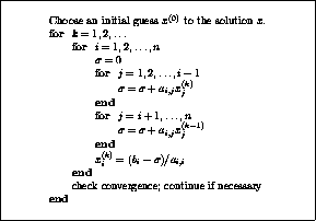
Figure: The Gauss-Seidel Method
Next:
The Successive Overrelaxation
Up:
Stationary Iterative Methods
Previous:
Convergence of the
Jack Dongarra
Mon Nov 20 08:52:54 EST 1995
The Successive Overrelaxation Method
Next:
Choosing the Value
Up:
Stationary Iterative Methods
Previous:
The Gauss-Seidel Method
The Successive Overrelaxation Method, or SOR, is devised
by applying extrapolation to the Gauss-Seidel method. This
extrapolation takes the form of a weighted average between the
previous iterate and the computed Gauss-Seidel iterate successively
for each component:

(where
denotes a Gauss-Seidel iterate, and
is the
extrapolation factor). The
idea is to choose a value for
that will accelerate the rate
of convergence of the iterates to the solution.
In matrix terms, the SOR algorithm can be written as
follows:

The pseudocode for the SOR algorithm is given in Figure
.
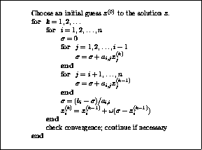
Figure: The SOR Method
Jack Dongarra
Mon Nov 20 08:52:54 EST 1995
Choosing the Value of <IMG ALIGN=BOTTOM SRC="http://www.netlib.org/utk/papers/templates/_22900_tex2html_wrap4973.gif">
Next:
The Symmetric Successive
Up:
The Successive Overrelaxation
Previous:
The Successive Overrelaxation
If  , the SOR method simplifies
to the Gauss-Seidel method. A theorem due to
Kahan
[130] shows that SOR fails to
converge if
is outside the interval
, the SOR method simplifies
to the Gauss-Seidel method. A theorem due to
Kahan
[130] shows that SOR fails to
converge if
is outside the interval  . Though
technically the term underrelaxation
should be used when
. Though
technically the term underrelaxation
should be used when  , for convenience the term
overrelaxation
is now used for any value
of
, for convenience the term
overrelaxation
is now used for any value
of  .
.
In general, it is not possible to compute in advance the value
of
that is optimal with respect to the rate of convergence of
SOR. Even when it is possible to compute the optimal value
for
, the expense of such computation is usually prohibitive.
Frequently, some heuristic estimate is used, such as  where
is the mesh spacing of the discretization of the
underlying physical domain.
where
is the mesh spacing of the discretization of the
underlying physical domain.
If the coefficient matrix
is symmetric and positive definite, the
SOR iteration is guaranteed to converge for any
value of
between 0 and 2, though the choice of
can
significantly affect the rate at which the SOR iteration
converges. Sophisticated implementations of the SOR
algorithm (such as that found in ITPACK
[140]) employ adaptive
parameter estimation schemes to try to home in on the appropriate
value of
by estimating the rate at which the iteration is
converging.
Adaptive methods: Iterative methods that collect information
about the coefficient matrix during the iteration process, and use
this to speed up convergence.
Symmetric matrix: See: Matrix properties.
Diagonally dominant matrix: See: Matrix properties
-Matrix: See: Matrix properties.
Positive definite matrix: See: Matrix properties.
Matrix properties: We call a square matrix
- Symmetric
- if
for all
,
.
- Positive definite
- if it satisfies
for all nonzero vectors
.
- Diagonally dominant
- if
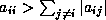 .
.
- An
-matrix
- if
for
, and it
is nonsingular with
for all
,
.
For coefficient matrices of a special class called consistently
ordered with property A (see
Young
[217]), which includes certain orderings of matrices
arising from the discretization of elliptic PDEs, there is a direct
relationship between the spectra of the Jacobi
and SOR iteration matrices. In principle, given the
spectral radius  of the
Jacobi iteration matrix, one can determine a priori the theoretically optimal value of
for SOR:
of the
Jacobi iteration matrix, one can determine a priori the theoretically optimal value of
for SOR:

This is seldom done, since calculating the spectral radius of the
Jacobi matrix requires an impractical amount of computation. However,
relatively inexpensive rough estimates of
(for example, from
the power method, see Golub and Van Loan [p. 351]GoVL:matcomp)
can yield reasonable estimates for the optimal value of
.
Next:
The Symmetric Successive
Up:
The Successive Overrelaxation
Previous:
The Successive Overrelaxation
Jack Dongarra
Mon Nov 20 08:52:54 EST 1995
The Symmetric Successive Overrelaxation Method
Next:
Notes and References
Up:
Stationary Iterative Methods
Previous:
Choosing the Value
If we assume that the coefficient matrix
is symmetric, then the
Symmetric Successive Overrelaxation method, or SSOR, combines two SOR
sweeps together in such a way that the resulting iteration matrix is
similar to a symmetric matrix. Specifically, the
first SOR sweep is carried out as
in (
), but in the second sweep the unknowns are
updated in the reverse order. That is, SSOR is a forward
SOR sweep followed by a
backward SOR sweep. The
similarity of the SSOR iteration matrix to a symmetric
matrix permits the application of SSOR as a preconditioner
for other iterative schemes for symmetric matrices. Indeed, this is
the primary motivation for SSOR since its convergence
rate
, with an optimal value of
, is
usually slower than the convergence rate of SOR with
optimal
(see Young [page 462]Yo:book). For details on
using SSOR as a preconditioner, see
Chapter
.
In matrix terms, the SSOR iteration can be expressed as
follows:

where

and

Note that  is simply the iteration matrix for SOR
from (
), and that
is simply the iteration matrix for SOR
from (
), and that  is the same, but with the
roles of
and
reversed.
is the same, but with the
roles of
and
reversed.
The pseudocode for the SSOR algorithm is given in
Figure
.
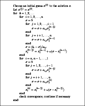
Figure: The SSOR Method
Jack Dongarra
Mon Nov 20 08:52:54 EST 1995
Notes and References
Next:
Nonstationary Iterative Methods
Up:
Stationary Iterative Methods
Previous:
The Symmetric Successive
The modern treatment of iterative methods dates back to the
relaxation
method of Southwell
[193].
This was the precursor to the SOR method, though the order in which
approximations to the unknowns were relaxed varied during the
computation. Specifically, the next unknown was chosen based upon
estimates of the location of the largest error in the current
approximation. Because of this, Southwell's relaxation method was
considered impractical for automated computing. It is interesting to
note that the introduction of multiple-instruction, multiple
data-stream (MIMD) parallel computers has rekindled an interest in
so-called asynchronous
, or chaotic
iterative methods (see Chazan and
Miranker
[54], Baudet
[30], and
Elkin
[92]), which are closely related to Southwell's
original relaxation method. In chaotic methods, the order of
relaxation is unconstrained, thereby eliminating costly
synchronization of the processors, though the effect on convergence is
difficult to predict.
The notion of accelerating the convergence of an iterative method by
extrapolation predates the development of SOR. Indeed, Southwell used
overrelaxation to accelerate the convergence of
his original relaxation method
. More
recently, the ad hoc SOR
method, in
which a different relaxation factor
is used for updating each
variable, has given impressive results for some classes of
problems (see Ehrlich
[83]).
The three main references for the theory of stationary iterative
methods are Varga
[211], Young
[217] and Hageman and
Young
[120]. The reader is referred to these books (and
the references therein) for further details concerning the methods
described in this section.
Jack Dongarra
Mon Nov 20 08:52:54 EST 1995
Nonstationary Iterative Methods
Next:
Conjugate Gradient Method
Up:
Iterative Methods
Previous:
Notes and References
Nonstationary methods differ from stationary methods in that the
computations involve information that changes at each iteration.
Typically, constants are computed by taking inner products of
residuals or other vectors arising from the iterative method.
Jack Dongarra
Mon Nov 20 08:52:54 EST 1995
Author's Affiliations
Next:
Acknowledgments
Up:
Templates for the Solution
Previous:
How to Use
-
-
Richard Barrett
Los Alamos National Laboratory
-
-
Michael Berry
University of Tennessee, Knoxville
-
-
Tony Chan
University of California, Los Angeles
-
-
James Demmel
University of California, Berkeley
-
-
June Donato
Oak Ridge National Laboratory
-
-
Jack Dongarra
University of Tennessee, Knoxville
and Oak Ridge National Laboratory
-
-
Victor Eijkhout
University of California, Los Angeles
-
-
Roldan Pozo
National Institute of Standards and Technology
-
-
Charles Romine
Oak Ridge National Laboratory
-
-
Henk van der Vorst
Utrecht University, the Netherlands
Jack Dongarra
Mon Nov 20 08:52:54 EST 1995
Conjugate Gradient Method (CG)
Next:
Theory
Up:
Nonstationary Iterative Methods
Previous:
Nonstationary Iterative Methods
The Conjugate Gradient method is
an effective method for symmetric positive definite systems. It is
the oldest and best known of the nonstationary methods discussed
here. The method proceeds by generating vector sequences of iterates
(i.e., successive approximations to the solution), residuals
corresponding to the iterates, and search directions
used in updating
the iterates and residuals. Although the length of these sequences can
become large, only a small number of vectors needs to be kept in
memory. In every iteration of the method, two inner products are
performed in order to compute update scalars that are defined to
make the sequences satisfy certain orthogonality conditions. On a
symmetric positive definite linear system these conditions imply that
the distance to the true solution is minimized in some norm.
The iterates
are updated in each iteration by a multiple
 of the
search direction vector
:
of the
search direction vector
:

Correspondingly the residuals 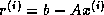 are updated as

The choice  minimizes
  over all possible choices for
  in
equation (
).
in
equation (
).
The search directions are updated using the residuals

where the choice 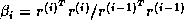 ensures
that
and
ensures
that
and  - or equivalently,
 and
and  - are orthogonal
. In fact, one can
show that this choice of
- are orthogonal
. In fact, one can
show that this choice of  makes
and
orthogonal to
all previous
makes
and
orthogonal to
all previous  and
and  respectively.
The pseudocode for the Preconditioned Conjugate Gradient Method is
given in Figure
. It uses a preconditioner
;
for  one obtains the unpreconditioned version of the Conjugate Gradient
Algorithm. In that case the algorithm may be further simplified by skipping
the ``solve'' line, and replacing
one obtains the unpreconditioned version of the Conjugate Gradient
Algorithm. In that case the algorithm may be further simplified by skipping
the ``solve'' line, and replacing  by
(and
by
(and  by
by  ).
).
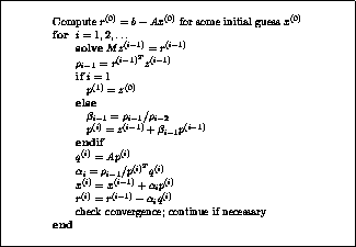
Figure: The Preconditioned Conjugate Gradient Method
Jack Dongarra
Mon Nov 20 08:52:54 EST 1995
Theory
Next:
Convergence
Up:
Conjugate Gradient Method
Previous:
Conjugate Gradient Method
The unpreconditioned conjugate gradient method constructs the
th
iterate
as an element of
 so that
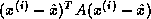 is minimized
, where
is the exact solution of
. This minimum is guaranteed
to exist in general only if
is symmetric positive definite. The
preconditioned version of the method uses a different subspace for
constructing the iterates, but it satisfies the same minimization
property, although over this different subspace. It requires in
addition that the preconditioner
is symmetric and positive
definite.
is minimized
, where
is the exact solution of
. This minimum is guaranteed
to exist in general only if
is symmetric positive definite. The
preconditioned version of the method uses a different subspace for
constructing the iterates, but it satisfies the same minimization
property, although over this different subspace. It requires in
addition that the preconditioner
is symmetric and positive
definite.
The above minimization of the error is equivalent to the residuals
being  orthogonal (that is,
 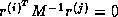 if
). Since for symmetric
an orthogonal basis for the Krylov subspace
if
). Since for symmetric
an orthogonal basis for the Krylov subspace
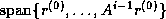 can be
constructed with only three-term recurrences
, such a recurrence also
suffices for generating the residuals. In the Conjugate
Gradient method two coupled two-term recurrences are used; one that
updates residuals using a search direction vector, and one updating
the search direction
with a newly computed residual.
This makes the
Conjugate Gradient Method quite attractive computationally.
can be
constructed with only three-term recurrences
, such a recurrence also
suffices for generating the residuals. In the Conjugate
Gradient method two coupled two-term recurrences are used; one that
updates residuals using a search direction vector, and one updating
the search direction
with a newly computed residual.
This makes the
Conjugate Gradient Method quite attractive computationally.
Krylov sequence: For a given matrix
and vector
, the
sequence of vectors
, or a finite initial part
of this sequence.
Krylov subspace: The subspace spanned by a Krylov sequence.
There is a close relationship between the Conjugate Gradient method
and the Lanczos method
for determining eigensystems, since both are
based on the construction of an orthogonal basis for the Krylov
subspace, and a similarity transformation of the coefficient matrix to
tridiagonal form. The coefficients computed during
the CG iteration then arise from the
factorization of this
tridiagonal matrix.
From the CG iteration one can reconstruct the Lanczos process, and vice versa;
see Paige and Saunders
[168]
and Golub and Van Loan [.2.6]GoVL:matcomp.
This relationship can be exploited to obtain relevant information
about the eigensystem of the (preconditioned) matrix
;
see §
.
Next:
Convergence
Up:
Conjugate Gradient Method
Previous:
Conjugate Gradient Method
Jack Dongarra
Mon Nov 20 08:52:54 EST 1995
Convergence
Next:
Implementation
Up:
Conjugate Gradient Method
Previous:
Theory
Accurate predictions of the convergence of iterative methods are
difficult to make, but useful bounds can often be obtained. For the
Conjugate Gradient method, the error can be
bounded in terms of the spectral condition number  of the
matrix
of the
matrix  . (Recall that if
and
are the largest and smallest eigenvalues of a
symmetric positive definite matrix
, then the spectral condition
number of
is
. (Recall that if
and
are the largest and smallest eigenvalues of a
symmetric positive definite matrix
, then the spectral condition
number of
is  . If
is the exact solution of the linear system
,
with symmetric positive definite matrix
, then for CG
with
symmetric positive definite preconditioner
, it can be shown that
. If
is the exact solution of the linear system
,
with symmetric positive definite matrix
, then for CG
with
symmetric positive definite preconditioner
, it can be shown that

where 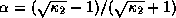 (see Golub and Van Loan
[][.2.8]GoVL:matcomp, and
Kaniel
[131]), and
(see Golub and Van Loan
[][.2.8]GoVL:matcomp, and
Kaniel
[131]), and
 . From this
relation we see that the number of iterations to reach a relative
reduction of
. From this
relation we see that the number of iterations to reach a relative
reduction of  in the error is proportional
to
in the error is proportional
to  .
.
In some cases, practical application of the above error bound is
straightforward. For example, elliptic second order partial
differential equations typically give rise to coefficient matrices
with  (where
is the discretization mesh
width), independent of the order of the finite elements or differences
used, and of the number of space dimensions of the problem (see for
instance Axelsson and Barker [.5]AxBa:febook). Thus,
without preconditioning, we expect a number of iterations proportional
to
(where
is the discretization mesh
width), independent of the order of the finite elements or differences
used, and of the number of space dimensions of the problem (see for
instance Axelsson and Barker [.5]AxBa:febook). Thus,
without preconditioning, we expect a number of iterations proportional
to  for the Conjugate Gradient method.
Other results concerning the behavior of the Conjugate Gradient
algorithm have been obtained. If the extremal eigenvalues of the
matrix
are well separated, then one often observes so-called
(see Concus, Golub and
O'Leary
[58]); that is, convergence at a
rate that increases per iteration.
This phenomenon is explained by
the fact that CG tends to eliminate components of the error in the
direction of eigenvectors associated with extremal eigenvalues first.
After these have been eliminated, the method proceeds as if these
eigenvalues did not exist in the given system, i.e., the
convergence rate depends on a reduced system with a (much) smaller
condition number (for an analysis of this, see Van der Sluis and
Van der Vorst
[199]). The effectiveness of
the preconditioner in reducing the condition number and in separating
extremal eigenvalues can be deduced by studying the approximated
eigenvalues of the related Lanczos process.
Next:
Implementation
Up:
Conjugate Gradient Method
Previous:
Theory
Jack Dongarra
Mon Nov 20 08:52:54 EST 1995
Implementation
Next:
Further references
Up:
Conjugate Gradient Method
Previous:
Convergence
The Conjugate Gradient method involves one matrix-vector product, three
vector updates, and two inner products per iteration. Some slight
computational variants exist that have the same
structure (see Reid
[179]). Variants that cluster the inner products
, a favorable property on
parallel machines, are discussed in §
.
For a discussion of the Conjugate Gradient method
on vector and shared
memory computers, see Dongarra, et
al.
[166]
[71]. For discussions
of the method for more general parallel architectures
see Demmel, Heath and Van der Vorst
[67] and
Ortega
[166], and the references therein.
Jack Dongarra
Mon Nov 20 08:52:54 EST 1995
Further references
Next:
MINRES and SYMMLQ
Up:
Conjugate Gradient Method
Previous:
Implementation
A more formal presentation of CG, as well as many theoretical
properties, can be found in the textbook by Hackbusch
[118].
Shorter presentations are given in Axelsson and Barker
[14]
and Golub and Van Loan
[109]. An overview of papers
published in the first 25 years of existence of the method is given
in Golub and O'Leary
[108].
Jack Dongarra
Mon Nov 20 08:52:54 EST 1995
MINRES and SYMMLQ
Next:
Theory
Up:
Nonstationary Iterative Methods
Previous:
Further references
The Conjugate Gradient method can be viewed as a special variant of
the Lanczos method
(see §
) for positive definite
symmetric systems. The MINRES
and SYMMLQ
methods are variants that can
be applied to symmetric indefinite systems.
The vector sequences in the Conjugate Gradient method
correspond to a
factorization of a tridiagonal matrix similar to the coefficient
matrix. Therefore, a breakdown
of the algorithm can occur
corresponding to a zero pivot if the matrix is indefinite.
Furthermore, for indefinite matrices the minimization property of the
Conjugate Gradient method
is no longer well-defined. The
MINRES
and SYMMLQ
methods are variants of the CG method that avoid the
-factorization and do not suffer from breakdown. MINRES
minimizes
the residual in the
-norm
. SYMMLQ solves the projected
system, but
does not minimize anything (it keeps the residual orthogonal to all
previous ones
). The convergence
behavior of Conjugate Gradients and MINRES
for indefinite systems was
analyzed by Paige, Parlett, and Van der Vorst
[167].
Breakdown: The occurrence of a zero coefficient that is
to be used as a divisor in an iterative method.
Jack Dongarra
Mon Nov 20 08:52:54 EST 1995
Theory
Next:
CG on the
Up:
MINRES and SYMMLQ
Previous:
MINRES and SYMMLQ
When
is not positive definite, but symmetric, we can still
construct an orthogonal basis for the Krylov subspace
by three term recurrence relations.
Eliminating the
search directions
in equations (
)
and (
) gives a recurrence

which can be written in matrix form as

where  is an
is an  tridiagonal matrix
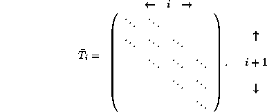
In this case we have the problem that  no
longer defines an inner product. However we can still try to minimize
the residual in the
-norm by obtaining
no
longer defines an inner product. However we can still try to minimize
the residual in the
-norm by obtaining

that minimizes

Now we exploit the fact that if  , then
 is an orthonormal transformation with respect to
the current Krylov subspace:
is an orthonormal transformation with respect to
the current Krylov subspace:

and this final expression can simply be seen as a minimum norm least
squares problem.
The element in the  position of
can be
annihilated by a simple Givens rotation and the resulting upper
bidiagonal system (the other subdiagonal elements having been removed
in previous iteration steps) can simply be solved, which leads to the
MINRES method (see Paige and Saunders
[168]).
position of
can be
annihilated by a simple Givens rotation and the resulting upper
bidiagonal system (the other subdiagonal elements having been removed
in previous iteration steps) can simply be solved, which leads to the
MINRES method (see Paige and Saunders
[168]).
Another possibility is to solve the system
 , as in the CG method (
 is the upper
 part of
). Other than in CG we cannot rely on
the existence of a Cholesky decomposition
(since
is not positive
definite). An alternative is then to decompose
by an
-decomposition. This again leads to simple recurrences and the
resulting method is known as SYMMLQ (see Paige and Saunders
[168]).
part of
). Other than in CG we cannot rely on
the existence of a Cholesky decomposition
(since
is not positive
definite). An alternative is then to decompose
by an
-decomposition. This again leads to simple recurrences and the
resulting method is known as SYMMLQ (see Paige and Saunders
[168]).
Jack Dongarra
Mon Nov 20 08:52:54 EST 1995
CG on the Normal Equations, CGNE and CGNR
Next:
Theory
Up:
Nonstationary Iterative Methods
Previous:
Theory
The CGNE
and CGNR methods
are the simplest methods for nonsymmetric or
indefinite systems. Since other methods for such systems are in
general rather more complicated than the Conjugate Gradient method,
transforming the system to a symmetric definite one and then applying
the Conjugate Gradient method is attractive for its coding simplicity.
Jack Dongarra
Mon Nov 20 08:52:54 EST 1995
Theory
Next:
Generalized Minimal Residual
Up:
CG on the
Previous:
CG on the
If a system of linear equations
has a nonsymmetric, possibly
indefinite (but nonsingular), coefficient matrix, one obvious attempt
at a solution is to apply Conjugate Gradient to a related symmetric positive definite system,
. While
this approach is easy to understand and code, the convergence speed of
the Conjugate Gradient method now depends on the square of the
condition number of the original coefficient matrix. Thus the
rate of convergence of the CG procedure on the normal equations
may be slow.
Several proposals have been made to improve the numerical stability of
this method. The best known is by Paige and Saunders
[169]
and is based upon applying the Lanczos method
to the auxiliary system
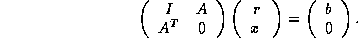
A clever execution of this scheme delivers the factors
and
of the
-decomposition of the tridiagonal matrix that would
have been computed by carrying out the Lanczos procedure with
.
Another means for improving the numerical stability of this normal
equations approach is suggested by Björck and Elfving in
[34].
The observation that the matrix
is used in the construction of
the iteration coefficients through an inner product like  leads to the suggestion that such an inner product
be replaced by
leads to the suggestion that such an inner product
be replaced by  .
.
Jack Dongarra
Mon Nov 20 08:52:54 EST 1995
Generalized Minimal Residual (GMRES)
Next:
Theory
Up:
Nonstationary Iterative Methods
Previous:
Theory
The Generalized Minimal Residual method
[189]
is an extension of MINRES
(which is only applicable to symmetric systems) to unsymmetric
systems. Like MINRES, it generates a sequence of orthogonal vectors,
but in the absence of symmetry this can no longer be done with short
recurrences; instead, all previously computed vectors in the
orthogonal sequence have to be retained. For this reason,
``restarted
'' versions of the method are used.
In the Conjugate Gradient method, the residuals form an orthogonal
basis
for the space  . In GMRES, this
basis is formed explicitly:
. In GMRES, this
basis is formed explicitly:
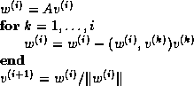
The reader may recognize this as a modified Gram-Schmidt
orthogonalization.
Applied to the Krylov
sequence
 this orthogonalization
is called the ``Arnoldi method''
[6].
The inner product coefficients
this orthogonalization
is called the ``Arnoldi method''
[6].
The inner product coefficients  and
and
 are stored in an upper Hessenberg matrix.
The GMRES iterates are constructed as

where the coefficients  have been chosen to minimize the residual
norm
have been chosen to minimize the residual
norm  . The GMRES algorithm has the property that this
residual norm can be computed without the iterate having been formed.
Thus, the expensive action of forming the iterate can be postponed
until the residual norm is deemed small enough.
. The GMRES algorithm has the property that this
residual norm can be computed without the iterate having been formed.
Thus, the expensive action of forming the iterate can be postponed
until the residual norm is deemed small enough.
The pseudocode for the restarted
GMRES(
) algorithm with preconditioner
is given in
Figure
.
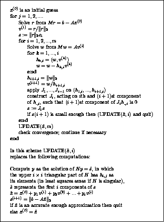
Figure: The Preconditioned GMRES Method
Jack Dongarra
Mon Nov 20 08:52:54 EST 1995
Acknowledgments
Next:
Contents
Up:
Templates for the Solution
Previous:
Author's Affiliations
The authors gratefully acknowledge the valuable assistance of many
people who commented on preliminary drafts of this book. In
particular, we thank Loyce Adams, Bill Coughran,
Matthew Fishler, Peter Forsyth,
Roland Freund, Gene
Golub, Eric Grosse, Mark Jones, David Kincaid, Steve Lee, Tarek
Mathew, Noël Nachtigal, Jim Ortega, and David Young for their
insightful comments. We also thank Geoffrey Fox for initial
discussions on the concept of templates, and Karin Remington for
designing the front cover.
This work was supported in part by DARPA and ARO under contract number
DAAL03-91-C-0047, the National Science Foundation Science and
Technology Center Cooperative Agreement No. CCR-8809615, the Applied
Mathematical Sciences subprogram of the Office of Energy Research,
U.S. Department of Energy, under Contract DE-AC05-84OR21400, and the
Stichting Nationale Computer Faciliteit (NCF) by Grant CRG 92.03.
Jack Dongarra
Mon Nov 20 08:52:54 EST 1995
Theory
Next:
Implementation
Up:
Generalized Minimal Residual
Previous:
Generalized Minimal Residual
The Generalized Minimum
Residual (GMRES) method
is designed to solve nonsymmetric linear
systems (see Saad and Schultz
[189]). The most popular
form of GMRES is based on the modified Gram-Schmidt procedure, and
uses restarts
to control storage requirements.
If no restarts are used, GMRES
(like any orthogonalizing Krylov-subspace method) will
converge in no more than
steps (assuming exact arithmetic). Of
course this is of no practical value when
is large; moreover, the
storage and computational requirements in the absence of restarts are
prohibitive. Indeed, the crucial element for successful application
of GMRES(
) revolves around the decision of when to restart; that
is, the choice of
. Unfortunately, there exist examples for which
the method stagnates
and convergence takes place only
at the
th step. For such systems, any choice of
less than
fails to converge.
Saad and Schultz
[189] have proven several useful results.
In particular, they show that if the coefficient matrix
is real
and nearly positive definite, then a ``reasonable'' value for
may be selected. Implications of the choice of
are discussed
below.
Jack Dongarra
Mon Nov 20 08:52:54 EST 1995
Implementation
Next:
BiConjugate Gradient (BiCG)
Up:
Generalized Minimal Residual
Previous:
Theory
A common implementation of GMRES
is suggested by Saad and Schultz in
[189] and
relies on using modified Gram-Schmidt orthogonalization. Householder
transformations, which are relatively costly but stable, have also
been proposed. The Householder approach results in a three-fold
increase in work associated with inner products and
vector updates (not with matrix vector products);
however, convergence may be better, especially for
ill-conditioned systems
(see Walker
[214]). From
the point of view of parallelism
, Gram-Schmidt orthogonalization may be
preferred, giving up some stability for better parallelization
properties (see Demmel, Heath and Van der Vorst
[67]).
Here we adopt the Modified Gram-Schmidt approach.
The major drawback to GMRES is that the amount of work and storage
required per iteration rises linearly with the iteration count.
Unless one is fortunate enough to obtain extremely fast convergence,
the cost will rapidly become prohibitive. The usual way to overcome
this limitation is by restarting
the iteration. After a chosen number
(
) of iterations, the accumulated data are cleared and the
intermediate results are used as the initial data for the next
iterations. This procedure is repeated until convergence is
achieved. The difficulty is in choosing an appropriate value for
.
If
is ``too small'', GMRES(
) may be slow to converge, or fail
to converge entirely. A value of
that is larger than necessary
involves excessive work (and uses more storage). Unfortunately, there
are no definite rules governing the choice of
-choosing when to
restart is a matter of experience.
For a discussion of GMRES for vector and shared memory computers see
Dongarra et al.
[71]; for more general
architectures,
see Demmel, Heath and Van der Vorst
[67]
.
Jack Dongarra
Mon Nov 20 08:52:54 EST 1995
BiConjugate Gradient (BiCG)
Next:
Convergence
Up:
Nonstationary Iterative Methods
Previous:
Implementation
The Conjugate Gradient method is not suitable for nonsymmetric systems
because the residual vectors cannot be made orthogonal with short
recurrences (for proof of this see Voevodin
[213] or Faber and
Manteuffel
[96]). The GMRES method retains
orthogonality of the residuals by using long recurrences, at the cost
of a larger storage demand. The BiConjugate Gradient method takes
another approach, replacing the orthogonal sequence of residuals by
two mutually orthogonal sequences, at the price of no longer providing
a minimization.
The update relations for residuals in the Conjugate Gradient method
are augmented in the BiConjugate Gradient method by relations
that are similar
but based on
instead of
. Thus we update two sequences of
residuals

and two sequences of search directions

The choices
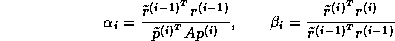
ensure the bi-orthogonality
relations

The pseudocode for the Preconditioned BiConjugate Gradient
Method with preconditioner
is given in Figure
.
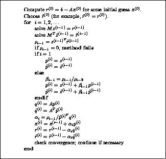
Figure: The Preconditioned BiConjugate Gradient Method
Jack Dongarra
Mon Nov 20 08:52:54 EST 1995
Convergence
Next:
Implementation
Up:
BiConjugate Gradient (BiCG)
Previous:
BiConjugate Gradient (BiCG)
Few theoretical results are known about the convergence of BiCG. For
symmetric positive definite systems the method delivers the same
results as CG, but at twice the cost per iteration. For nonsymmetric
matrices it has been shown that in phases of the process where there
is significant reduction of the norm of the residual, the method is
more or less comparable to full GMRES
(in terms of numbers of
iterations) (see Freund and Nachtigal
[102]). In practice
this is often confirmed, but
it is also observed that the convergence behavior may be quite
irregular
, and the method may even break
down
. The breakdown
situation due to the possible event that
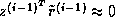 can be circumvented by so-called
look-ahead strategies
(see Parlett, Taylor and Liu
[172]). This
leads to
complicated codes and is beyond the scope of this book. The other
breakdown
situation,
can be circumvented by so-called
look-ahead strategies
(see Parlett, Taylor and Liu
[172]). This
leads to
complicated codes and is beyond the scope of this book. The other
breakdown
situation,  ,
occurs when the
-decomposition fails (see the theory subsection
of §
), and can be repaired by
using another decomposition. This is done in the version of QMR
that we adopted
(see §
).
,
occurs when the
-decomposition fails (see the theory subsection
of §
), and can be repaired by
using another decomposition. This is done in the version of QMR
that we adopted
(see §
).
Sometimes, breakdown
or near-breakdown situations can be
satisfactorily avoided by a restart
at the iteration step immediately
before the (near-) breakdown step. Another possibility is to switch to
a more robust (but possibly more expensive) method, like GMRES.
Jack Dongarra
Mon Nov 20 08:52:54 EST 1995
Implementation
Next:
Quasi-Minimal Residual (QMR)
Up:
BiConjugate Gradient (BiCG)
Previous:
Convergence
BiCG requires computing a matrix-vector product  and a
transpose product
and a
transpose product  . In some applications the
latter product may be impossible to perform, for instance if the
matrix is not formed explicitly
and the regular product is only given in operation form, for instance
as a function call evaluation.
. In some applications the
latter product may be impossible to perform, for instance if the
matrix is not formed explicitly
and the regular product is only given in operation form, for instance
as a function call evaluation.
In a parallel environment
, the two matrix-vector products can
theoretically be performed simultaneously; however,
in a distributed-memory environment, there will be extra communication
costs associated with one of the two matrix-vector products, depending
upon the storage scheme for
.
A duplicate copy of the
matrix will alleviate this problem, at the cost of doubling the
storage requirements for the matrix.
Care must also be exercised in choosing the preconditioner, since
similar problems arise during the two solves involving the
preconditioning matrix.
It is difficult to make a fair comparison between GMRES
and BiCG.
GMRES really minimizes a residual, but at the cost of increasing work
for keeping all residuals orthogonal and increasing demands for memory
space. BiCG does not minimize a residual, but often its
accuracy is comparable to GMRES, at the cost of twice the amount of matrix
vector products per iteration step. However, the generation of the
basis vectors is relatively cheap and the memory requirements are
modest. Several variants of BiCG have been proposed that increase
the effectiveness of this class of methods in certain circumstances. These
variants (CGS and Bi-CGSTAB) will be discussed in coming subsections.
Jack Dongarra
Mon Nov 20 08:52:54 EST 1995
Quasi-Minimal Residual (QMR)
Next:
Convergence
Up:
Nonstationary Iterative Methods
Previous:
Implementation
The BiConjugate Gradient method often displays rather irregular
convergence
behavior. Moreover, the implicit
decomposition of the
reduced tridiagonal system may not exist, resulting in breakdown
of the algorithm. A related algorithm, the
Quasi-Minimal Residual method of Freund and
Nachtigal
[102],
[103]
attempts to overcome
these problems. The main idea behind this algorithm is to solve the
reduced tridiagonal system in a least squares sense, similar to the
approach followed in GMRES.
Since the constructed basis for the
Krylov subspace
is bi-orthogonal
, rather than orthogonal as in GMRES,
the obtained solution is viewed as a quasi-minimal residual solution,
which explains the name. Additionally, QMR uses look-ahead techniques
to avoid breakdowns in the underlying Lanczos process, which makes it
more robust than BiCG.
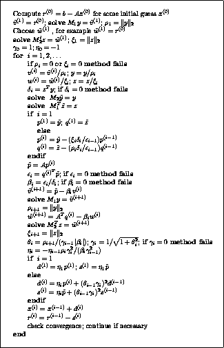
Figure: The Preconditioned Quasi Minimal Residual Method
without Look-ahead
Jack Dongarra
Mon Nov 20 08:52:54 EST 1995
Convergence
Next:
Implementation
Up:
Quasi-Minimal Residual (QMR)
Previous:
Quasi-Minimal Residual (QMR)
The convergence behavior of QMR
is typically much smoother than for BiCG.
Freund and Nachtigal
[102] present quite general error
bounds which show that
QMR may be expected to converge about as fast as GMRES. From a relation
between the residuals in BiCG and QMR
(Freund and Nachtigal [relation (5.10)]FrNa:qmr) one may deduce
that at phases in the
iteration process where BiCG makes significant progress, QMR has arrived
at about the same approximation for
.
On the other hand, when BiCG makes
no progress at all
, QMR may still show slow convergence.
The look-ahead steps in the version of the QMR method
discussed in
[102] prevents breakdown in all cases
but the so-called ``incurable breakdown'', where no practical number of
look-ahead steps would yield a next iterate.
Jack Dongarra
Mon Nov 20 08:52:54 EST 1995
Implementation
Next:
Conjugate Gradient Squared
Up:
Quasi-Minimal Residual (QMR)
Previous:
Convergence
The pseudocode for the Preconditioned Quasi Minimal Residual
Method, with preconditioner  ,
is given in Figure
.
This algorithm follows the two term recurrence
version
without look-ahead, presented by Freund and
Nachtigal
[103] as Algorithm 7.1.
This version of QMR is simpler to implement than the full QMR method
with look-ahead, but it is susceptible to breakdown of the underlying
Lanczos process. (Other implementational variations are whether to
scale Lanczos vectors or not, or to use three-term recurrences instead
of coupled two-term recurrences. Such decisions usually have implications
for the stability and the efficiency of the algorithm.)
A professional implementation of QMR
with look-ahead is given in Freund and Nachtigal's QMRPACK, which
is available through netlib; see Appendix
.
,
is given in Figure
.
This algorithm follows the two term recurrence
version
without look-ahead, presented by Freund and
Nachtigal
[103] as Algorithm 7.1.
This version of QMR is simpler to implement than the full QMR method
with look-ahead, but it is susceptible to breakdown of the underlying
Lanczos process. (Other implementational variations are whether to
scale Lanczos vectors or not, or to use three-term recurrences instead
of coupled two-term recurrences. Such decisions usually have implications
for the stability and the efficiency of the algorithm.)
A professional implementation of QMR
with look-ahead is given in Freund and Nachtigal's QMRPACK, which
is available through netlib; see Appendix
.
We have modified Algorithm 7.1 in
[103] to include a
relatively inexpensive recurrence relation for the computation
of the residual vector. This requires a few extra vectors of storage
and vector update operations per iteration, but it avoids expending
a matrix-vector product on the residual calculation.
Also, the algorithm has been modified so that only two
full preconditioning steps are required instead of three.
Computation of the residual is done for the convergence test.
If one uses right (or post) preconditioning, that is  , then a
cheap upper bound for
, then a
cheap upper bound for  can be computed in each iteration,
avoiding the recursions for
. For details,
see Freund and Nachtigal [proposition 4.1]FrNa:qmr. This upper
bound may be
pessimistic by a factor of at most
can be computed in each iteration,
avoiding the recursions for
. For details,
see Freund and Nachtigal [proposition 4.1]FrNa:qmr. This upper
bound may be
pessimistic by a factor of at most  .
.
QMR has roughly the same problems with respect to vector and parallel
implementation as BiCG. The scalar overhead per iteration is slightly
more than for BiCG. In all cases where the slightly cheaper BiCG method
converges irregularly
(but fast enough),
QMR may be preferred for stability reasons.
Jack Dongarra
Mon Nov 20 08:52:54 EST 1995
Conjugate Gradient Squared Method (CGS)
Next:
Convergence
Up:
Nonstationary Iterative Methods
Previous:
Implementation
In BiCG, the residual vector
can be regarded as
the product
of
and an
th degree polynomial in
, that is

This same polynomial satisfies
 so that

This suggests that if  reduces
to a smaller
vector
, then it might be advantageous to apply this
``contraction'' operator twice, and compute
reduces
to a smaller
vector
, then it might be advantageous to apply this
``contraction'' operator twice, and compute  .
Equation (
) shows that the iteration coefficients can
still be recovered from these vectors, and it turns out to be easy to
find the corresponding approximations for
. This
approach leads to the Conjugate Gradient Squared method (see
Sonneveld
[192]).
.
Equation (
) shows that the iteration coefficients can
still be recovered from these vectors, and it turns out to be easy to
find the corresponding approximations for
. This
approach leads to the Conjugate Gradient Squared method (see
Sonneveld
[192]).

Figure: The Preconditioned Conjugate Gradient Squared Method
Jack Dongarra
Mon Nov 20 08:52:54 EST 1995
Convergence
Next:
Implementation
Up:
Conjugate Gradient Squared
Previous:
Conjugate Gradient Squared
Often one observes a speed of convergence for CGS that is about twice
as fast as for BiCG, which is in agreement with the observation that
the same ``contraction'' operator is applied twice. However, there is
no reason that the ``contraction'' operator, even if it really reduces
the initial residual
, should also reduce the once reduced
vector  . This is evidenced by the often
highly irregular convergence behavior of CGS
. One should be aware of
the fact that local corrections to the current solution may be so
large that cancelation effects occur. This may lead to a less
accurate solution than suggested by the updated residual
(see Van der Vorst
[207]).
The method tends to diverge if the starting guess is close to the solution.
. This is evidenced by the often
highly irregular convergence behavior of CGS
. One should be aware of
the fact that local corrections to the current solution may be so
large that cancelation effects occur. This may lead to a less
accurate solution than suggested by the updated residual
(see Van der Vorst
[207]).
The method tends to diverge if the starting guess is close to the solution.
Jack Dongarra
Mon Nov 20 08:52:54 EST 1995
Contents
Next:
List of Figures
Up:
Templates for the Solution
Previous:
Acknowledgments
Jack Dongarra
Mon Nov 20 08:52:54 EST 1995
Implementation
Next:
BiConjugate Gradient Stabilized
Up:
Conjugate Gradient Squared
Previous:
Convergence
CGS requires about the same number of
operations per iteration as
BiCG, but does not involve computations with
. Hence, in
circumstances where computation with
is impractical, CGS may be
attractive.
The pseudocode for the Preconditioned Conjugate Gradient Squared
Method with preconditioner
is given in Figure
.
Jack Dongarra
Mon Nov 20 08:52:54 EST 1995
BiConjugate Gradient Stabilized (Bi-CGSTAB)
Next:
Convergence
Up:
Nonstationary Iterative Methods
Previous:
Implementation
The BiConjugate Gradient Stabilized method (Bi-CGSTAB) was developed to
solve nonsymmetric linear systems while avoiding the often irregular
convergence
patterns of the Conjugate
Gradient Squared
method (see Van der Vorst
[207]). Instead of computing
the CGS sequence
 , Bi-CGSTAB computes
 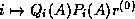 where
where  is an
th degree polynomial describing a steepest
descent update.
is an
th degree polynomial describing a steepest
descent update.
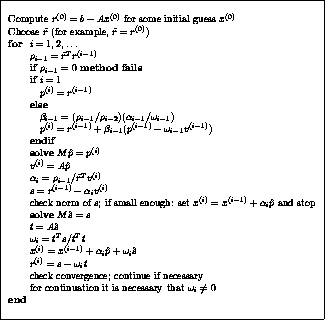
Figure: The Preconditioned BiConjugate Gradient Stabilized Method
Jack Dongarra
Mon Nov 20 08:52:54 EST 1995
Convergence
Next:
Implementation
Up:
BiConjugate Gradient Stabilized
Previous:
BiConjugate Gradient Stabilized
Bi-CGSTAB often converges about as fast as CGS,
sometimes faster and
sometimes not. CGS can be viewed as a method in which the BiCG
``contraction'' operator is applied twice. Bi-CGSTAB can be
interpreted as the product of BiCG and repeatedly applied GMRES(1). At
least locally, a residual vector is minimized
, which leads to a
considerably smoother
convergence behavior. On the
other hand, if the
local GMRES(1) step stagnates, then the Krylov subspace
is not
expanded, and Bi-CGSTAB will break down
. This is a breakdown situation
that can occur in addition to the other breakdown possibilities in the
underlying BiCG algorithm. This type of breakdown may be avoided by
combining BiCG with other methods, i.e., by selecting other
values for  (see the algorithm). One such alternative is
Bi-CGSTAB2
(see Gutknecht
[115]); more general
approaches are suggested by Sleijpen and Fokkema in
[190].
(see the algorithm). One such alternative is
Bi-CGSTAB2
(see Gutknecht
[115]); more general
approaches are suggested by Sleijpen and Fokkema in
[190].
Note that Bi-CGSTAB has two stopping tests: if the method has already
converged at the first test on the norm of
, the subsequent update
would be numerically questionable. Additionally, stopping on the first
test saves a few unnecessary operations, but this is of minor importance.
Jack Dongarra
Mon Nov 20 08:52:54 EST 1995
Implementation
Next:
Chebyshev Iteration
Up:
BiConjugate Gradient Stabilized
Previous:
Convergence
Bi-CGSTAB requires two matrix-vector products
and four inner products, i.e., two inner products more than BiCG
and CGS.
The pseudocode for the Preconditioned BiConjugate Gradient Stabilized
Method with preconditioner
is given in Figure
.
Jack Dongarra
Mon Nov 20 08:52:54 EST 1995
Chebyshev Iteration
Next:
Comparison with other
Up:
Nonstationary Iterative Methods
Previous:
Implementation
Chebyshev Iteration is another method for solving
nonsymmetric
problems (see Golub and
Van Loan [.1.5]GoVL:matcomp and
Varga [Chapter 5]Va:book).
Chebyshev Iteration avoids the computation of inner products
as is
necessary for the other nonstationary methods.
For some distributed memory architectures
these inner products are a bottleneck
with respect to efficiency. The
price one pays for avoiding inner products is that the method requires
enough knowledge about the spectrum of the coefficient matrix
that
an ellipse enveloping the spectrum can be identified
;
however this
difficulty can be overcome via an adaptive construction
developed by
Manteuffel
[146], and implemented by Ashby
[7].
Chebyshev iteration is suitable for any nonsymmetric linear system for
which the enveloping ellipse does not include the origin.
Jack Dongarra
Mon Nov 20 08:52:54 EST 1995
Comparison with other methods
Next:
Convergence
Up:
Chebyshev Iteration
Previous:
Chebyshev Iteration
Comparing the pseudocode for Chebyshev Iteration with the pseudocode
for the Conjugate Gradient method shows a high degree of similarity,
except that no inner products are computed in Chebyshev Iteration
.
Scalars
and
must be selected so that they define a family of
ellipses
with common center  and foci
  and
and  which contain the
ellipse that encloses the spectrum (or more general, field of values)
of
and for which the rate
which contain the
ellipse that encloses the spectrum (or more general, field of values)
of
and for which the rate  of
convergence is minimal:
of
convergence is minimal:

where  is the length of the
-axis of the ellipse.
is the length of the
-axis of the ellipse.
We provide code in which it is assumed that
the ellipse degenerate to the interval  ,
that is all eigenvalues are real.
For code including the adaptive determination of the iteration
parameters
and
the reader is referred
to Ashby
[7].
,
that is all eigenvalues are real.
For code including the adaptive determination of the iteration
parameters
and
the reader is referred
to Ashby
[7].
The Chebyshev
method has the advantage over GMRES that only short recurrences are
used. On the other hand, GMRES is guaranteed to generate the smallest
residual over the current search space. The BiCG methods, which also
use short recurrences, do not minimize the residual in a suitable
norm; however, unlike Chebyshev iteration, they do not require
estimation of parameters (the spectrum of
). Finally, GMRES and
BiCG may be more effective in practice, because of superlinear
convergence behavior
, which cannot be expected for
Chebyshev.
For symmetric positive definite systems the ``ellipse'' enveloping the
spectrum degenerates to the interval
on the positive
-axis, where
and
are the smallest and largest eigenvalues of
. In circumstances where the computation of inner products
is a bottleneck
, it may be advantageous to start
with CG, compute
estimates of the extremal eigenvalues from the CG coefficients, and
then after sufficient convergence of these approximations switch to
Chebyshev Iteration
. A similar strategy
may be adopted for a switch from GMRES, or BiCG-type methods, to
Chebyshev Iteration.
Next:
Convergence
Up:
Chebyshev Iteration
Previous:
Chebyshev Iteration
Jack Dongarra
Mon Nov 20 08:52:54 EST 1995
Convergence
Next:
Implementation
Up:
Chebyshev Iteration
Previous:
Comparison with other
In the symmetric case (where
and the preconditioner
are both
symmetric) for the Chebyshev Iteration we have the same upper
bound as for the Conjugate Gradient
method, provided
and
are computed from
and
(the extremal eigenvalues of the preconditioned
matrix
).
There is a severe penalty for overestimating
or underestimating the field of values. For example, if in the
symmetric case
is underestimated, then the method may
diverge; if it is overestimated then the result may be very slow
convergence. Similar statements can be made for the nonsymmetric case.
This implies that one needs fairly accurate bounds on the
spectrum of
for the method to be effective (in comparison
with CG or GMRES).
Jack Dongarra
Mon Nov 20 08:52:54 EST 1995
Implementation
Next:
Computational Aspects of
Up:
Chebyshev Iteration
Previous:
Convergence
In Chebyshev Iteration the iteration parameters
are known as soon
as one knows the ellipse containing the eigenvalues (or rather, the
field of values) of the operator. Therefore the computation of
inner products, as is necessary in methods like GMRES or CG,
is avoided
.
This avoids the synchronization points required of CG-type methods, so
machines with hierarchical or distributed memory may achieve higher
performance (it also suggests strong parallelization properties
; for a
discussion of this see Saad
[185], and Dongarra, et
al.
[71]).
Specifically, as soon as some segment of
is computed, we may begin
computing, in sequence, corresponding segments of
,
, and
.
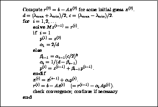
Figure: The Preconditioned Chebyshev Method
The pseudocode for the Preconditioned Chebyshev
Method with preconditioner
is given in Figure
.
It handles the case of a symmetric
positive definite coefficient matrix
. The
eigenvalues of
are assumed to be all real and in the
interval
, which does not include
zero.
Jack Dongarra
Mon Nov 20 08:52:54 EST 1995
Computational Aspects of the Methods
Next:
A short history
Up:
Iterative Methods
Previous:
Implementation
Efficient solution of a linear system is largely a function of the
proper choice of iterative method. However,
to obtain good performance, consideration must also be given to the
computational kernels of the method and how efficiently they can be
executed on the target architecture. This point is of particular
importance on parallel architectures; see §
.
Iterative methods are very different from direct methods in this
respect. The performance of direct methods, both for dense and sparse
systems, is largely that of the factorization of the matrix. This
operation is absent in iterative methods (although preconditioners may
require a setup phase), and with it, iterative methods lack dense
matrix suboperations. Since such operations can be executed at very
high efficiency on most current computer architectures, we expect a
lower flop rate for iterative than for direct methods.
(Dongarra and Van der Vorst
[74] give some
experimental results about this, and provide a benchmark code
for iterative solvers.)
Furthermore,
the basic operations in iterative methods often use indirect
addressing, depending on the data structure. Such operations also have
a relatively low efficiency of execution.
However, this lower efficiency of execution does not imply anything
about the total solution time for a given system. Furthermore,
iterative methods are usually simpler to implement than direct
methods, and since no full factorization has to be stored, they can
handle much larger systems than direct methods.
In this section we summarize for each method
- Matrix properties. Not every method will work on every problem
type, so knowledge of matrix properties is the main criterion for
selecting an iterative method.
- Computational kernels. Different methods involve different
kernels, and depending on the problem or target computer architecture
this may rule out certain methods.
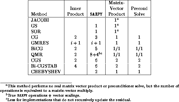
Table: Summary of Operations for Iteration
.
``a/b'' means ``a'' multiplications with the matrix and ``b'' with
its transpose.
Table
lists the storage required for each method
(without preconditioning). Note that we are not including the storage
for the original
system
and we ignore scalar storage.
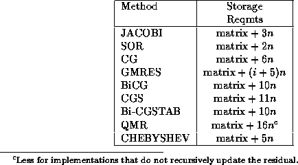
Table: Storage Requirements for the Methods in iteration
:
denotes the order of the matrix.
- Jacobi Method
- Extremely easy to use, but unless the matrix is ``strongly''
diagonally dominant, this method is probably best only considered
as an introduction to iterative methods or as a preconditioner in
a nonstationary method.
- Trivial to parallelize.
- Gauss-Seidel Method
- Typically faster convergence than Jacobi, but in general not
competitive with the nonstationary methods.
- Applicable to strictly diagonally dominant, or symmetric
positive definite matrices.
- Parallelization properties depend on structure of the
coefficient matrix. Different orderings of the unknowns have
different degrees of parallelism; multi-color orderings may give
almost full parallelism.
- This is a special case of the SOR method, obtained by
choosing
.
- Successive Over-Relaxation (SOR)
- Accelerates convergence of Gauss-Seidel (
 , over-relaxation); may yield convergence when Gauss-Seidel fails
(
, under-relaxation).
, over-relaxation); may yield convergence when Gauss-Seidel fails
(
, under-relaxation).
- Speed of convergence depends critically on
; the
optimal value for
may be estimated from the spectral
radius of the Jacobi iteration matrix under certain conditions.
- Parallelization properties are the same as those of the
Gauss-Seidel method.
- Conjugate Gradient (CG)
- Applicable to symmetric positive definite systems.
- Speed of convergence depends on the condition number; if
extremal eigenvalues are well-separated then superlinear
convergence behavior can result.
- Inner products act as synchronization points in a parallel
environment.
- Further parallel properties are largely independent of the
coefficient matrix, but depend strongly on the structure the
preconditioner.
- Generalized Minimal Residual (GMRES)
- Applicable to nonsymmetric matrices.
- GMRES leads to the smallest residual for a fixed number of
iteration steps, but these steps become increasingly expensive.
- In order to limit the increasing storage requirements and work
per iteration step, restarting is necessary. When to do so depends
on
and the right-hand side; it requires skill and experience.
- GMRES requires only matrix-vector products with the
coefficient matrix.
- The number of inner products grows linearly with the iteration
number, up to the restart point. In an implementation based on a
simple Gram-Schmidt process the inner products are independent, so
together they imply only one synchronization point. A more stable
implementation based on modified Gram-Schmidt orthogonalization
has one synchronization point per inner product.
- Biconjugate Gradient (BiCG)
- Applicable to nonsymmetric matrices.
- Requires matrix-vector products with the coefficient matrix
and its transpose. This disqualifies the method for cases where
the matrix is only given implicitly as an operator, since usually no
corresponding transpose operator is available in such cases.
- Parallelization properties are similar to those for CG; the
two matrix vector products (as well as the preconditioning steps)
are independent, so they can be done in parallel, or their
communication stages can be packaged.
- Quasi-Minimal Residual (QMR)
- Applicable to nonsymmetric matrices.
- Designed to avoid the irregular convergence behavior of BiCG,
it avoids one of the two breakdown situations of BiCG.
- If BiCG makes significant progress in one iteration step, then
QMR delivers about the same result at the same step. But when BiCG
temporarily stagnates or diverges, QMR may still further reduce
the residual, albeit very slowly.
- Computational costs per iteration are similar to BiCG, but slightly
higher. The method requires the transpose matrix-vector product.
- Parallelization properties are as for BiCG.
- Conjugate Gradient Squared (CGS)
- Applicable to nonsymmetric matrices.
- Converges (diverges) typically about twice as fast as BiCG.
- Convergence behavior is often quite irregular, which may lead
to a loss of accuracy in the updated residual.
- Computational costs per iteration are similar to BiCG, but the
method doesn't require the transpose matrix.
- Unlike BiCG, the two matrix-vector products are not
independent, so the number of synchronization points in a parallel
environment is larger.
- Biconjugate Gradient Stabilized (Bi-CGSTAB)
- Applicable to nonsymmetric matrices.
- Computational costs per iteration are similar to BiCG and CGS,
but the method doesn't require the transpose matrix.
- An alternative for CGS that avoids the irregular convergence
patterns of CGS while maintaining about the same speed of
convergence; as a result we often observe less loss of accuracy in
the updated residual.
- Chebyshev Iteration
- Applicable to nonsymmetric matrices (but presented in this
book only for the symmetric case).
- This method requires some explicit knowledge of the spectrum
(or field of values); in the symmetric case the iteration
parameters are easily obtained from the two extremal eigenvalues,
which can be estimated either directly from the matrix, or from
applying a few iterations of the Conjugate Gradient Method.
- The computational structure is similar to that of CG, but
there are no synchronization points.
- The Adaptive Chebyshev method can be used in combination with
methods as CG or GMRES, to continue the iteration once suitable
bounds on the spectrum have been obtained from these methods.
Selecting the ``best'' method for a given class of problems is largely
a matter of trial and error. It also depends on how much storage one
has available (GMRES), on the availability of
(BiCG and QMR),
and on how expensive the matrix vector products (and Solve steps with
) are in comparison to SAXPYs and inner products. If these matrix
vector products are relatively expensive, and if sufficient storage is
available then it may be attractive to use GMRES and delay restarting
as much as possible.
Table
shows the type of operations performed per
iteration. Based on the particular problem or data structure, the
user may observe that a particular operation could be performed more
efficiently.
Next:
A short history
Up:
Iterative Methods
Previous:
Implementation
Jack Dongarra
Mon Nov 20 08:52:54 EST 1995
A short history of Krylov
methods<A NAME=tex2html142 HREF="http://www.netlib.org/utk/papers/templates/footnode.html#3831">
<IMG ALIGN=BOTTOM ALT="gif" SRC="http://www.netlib.org/utk/icons/foot_motif.gif">
</A>
Next:
Survey of recent
Up:
Iterative Methods
Previous:
Computational Aspects of
Methods based on orthogonalization were developed by a number of
authors in the early '50s. Lanczos'
method
[142] was based on two mutually orthogonal
vector sequences, and his motivation came from eigenvalue problems. In
that context, the most prominent feature of the method is that it
reduces the original matrix to tridiagonal form. Lanczos
later applied his method to solving linear systems, in particular
symmetric ones
[143]. An important
property for proving convergence of the method when solving linear
systems is that the iterates are related to the initial residual by
multiplication with a polynomial in the coefficient matrix.
The joint paper by Hestenes
and Stiefel
[122], after their independent discovery
of the same method, is the classical description of the conjugate
gradient method for solving linear systems. Although error-reduction
properties are proved, and experiments showing premature convergence
are reported, the conjugate gradient method is presented here as a
direct method, rather than an iterative method.
This Hestenes/Stiefel method is closely related to a reduction of the
Lanczos method to symmetric matrices, reducing the two mutually
orthogonal sequences to one orthogonal sequence, but there is an
important algorithmic difference. Whereas Lanczos used three-term
recurrences, the method by Hestenes and Stiefel uses coupled two-term
recurrences. By combining the two two-term recurrences (eliminating
the ``search directions'') the Lanczos method is obtained.
A paper by
Arnoldi
[6] further discusses the Lanczos
biorthogonalization method, but it also presents a new method,
combining features of the Lanczos and Hestenes/Stiefel methods.
Like the Lanczos method it is applied to nonsymmetric systems, and
it does not use search directions. Like the Hestenes/Stiefel method,
it generates only one, self-orthogonal sequence. This last fact,
combined with the asymmetry of the coefficient matrix means that the
method no longer effects a reduction to tridiagonal form, but instead
one to upper Hessenberg form.
Presented as ``minimized iterations in the Galerkin method'' this
algorithm has become known as the Arnoldi algorithm.
The conjugate gradient method received little attention as a practical
method for some time, partly because of a misperceived importance of
the finite termination property. Reid
[179] pointed out that
the most important application area lay in sparse definite systems,
and this renewed the interest in the method.
Several methods have been developed in later years that employ, most
often implicitly, the upper Hessenberg matrix of the Arnoldi method.
For an overview and characterization of these orthogonal projection
methods for nonsymmetric systems
see Ashby, Manteuffel and Saylor
[10],
Saad and Schultz
[188], and Jea and
Young
[125].
Fletcher
[98] proposed an implementation of the
Lanczos method, similar to the Conjugate Gradient method, with two
coupled two-term recurrences, which he named the bi-conjugate
gradient method (BiCG).
Next:
Survey of recent
Up:
Iterative Methods
Previous:
Computational Aspects of
Jack Dongarra
Mon Nov 20 08:52:54 EST 1995
List of Figures
Next:
Introduction
Up:
Templates for the Solution
Previous:
Contents
Jack Dongarra
Mon Nov 20 08:52:54 EST 1995
Survey of recent Krylov methods
Next:
Preconditioners
Up:
Iterative Methods
Previous:
A short history
Research into the design of Krylov subspace methods for solving
nonsymmetric linear systems is an active field of research and new
methods are still emerging. In this book, we have included only the
best known and most popular methods, and in particular those for which
extensive computational experience has been gathered. In this
section, we shall briefly highlight some of the recent developments
and other methods not treated here. A survey of methods up to about
1991 can be found in Freund, Golub and
Nachtigal
[106]. Two more recent reports by
Meier-Yang
[151] and Tong
[197] have extensive
numerical comparisons among various methods, including several more
recent ones that have not been discussed in detail in this book.
Several suggestions have been made to reduce the increase in memory
and computational costs in GMRES. An obvious one is to restart (this one is included
in §
): GMRES(
). Another approach is to restrict
the GMRES search to a suitable subspace of some higher-dimensional
Krylov subspace. Methods based on this idea can be viewed as
preconditioned GMRES methods. The simplest ones exploit a fixed
polynomial preconditioner (see Johnson, Micchelli and
Paul
[126],
Saad
[183], and Nachtigal,
Reichel and Trefethen
[159]).
In more sophisticated approaches, the
polynomial preconditioner is adapted to the iterations
(Saad
[187]), or the preconditioner may even be some other
(iterative) method of choice (Van der Vorst and
Vuik
[209], Axelsson and
Vassilevski
[24]). Stagnation is prevented in the GMRESR
method (Van der Vorst and Vuik
[209]) by including
LSQR steps in some phases of the process. In De Sturler and
Fokkema
[64], part of the optimality of GMRES is
maintained in the hybrid method GCRO, in which the iterations of the
preconditioning method are kept orthogonal to the iterations of the
underlying GCR method. All these approaches have advantages for some
problems, but it is far from clear a priori which strategy is
preferable in any given case.
Recent work has focused on endowing
the BiCG method with several desirable properties:
(1) avoiding breakdown;
(2) avoiding use of the transpose;
(3) efficient use of matrix-vector products;
(4) smooth convergence; and
(5) exploiting the work expended in forming the Krylov space with
for further reduction of the residual.
As discussed before, the BiCG method can have two kinds
of breakdown: Lanczos breakdown (the underlying Lanczos
process breaks down), and pivot breakdown (the
tridiagonal matrix
implicitly generated in the
underlying Lanczos process encounters a zero pivot when
Gaussian elimination without pivoting is used to factor it).
Although such exact breakdowns are very rare in practice, near
breakdowns can cause severe numerical stability problems.
The pivot breakdown is the easier one to overcome and there have been
several approaches proposed in the literature. It should be noted
that for symmetric matrices, Lanczos breakdown cannot occur and the
only possible breakdown is pivot breakdown. The SYMMLQ and QMR
methods discussed in this book circumvent pivot breakdown by solving
least squares systems. Other methods tackling this problem can be
found
in Fletcher
[98], Saad
[181],
Gutknecht
[113], and Bank and
Chan
[29]
[28].
Lanczos breakdown is much more difficult to eliminate. Recently,
considerable attention has been given to analyzing the nature of the
Lanczos breakdown (see Parlett
[172], and
Gutknecht
[114]
[116]), as well as various look-ahead
techniques for remedying it (see Brezinski and
Sadok
[39], Brezinski, Zaglia and
Sadok
[41]
[40],
Freund and Nachtigal
[102], Parlett
[172],
Nachtigal
[160], Freund, Gutknecht and
Nachtigal
[101],
Joubert
[129], Freund, Golub
and Nachtigal
[106], and
Gutknecht
[114]
[116]). However, the resulting
algorithms are usually too complicated to give in template form (some
codes of Freund and Nachtigal are available on netlib.)
Moreover, it is still not possible to eliminate breakdowns that
require look-ahead steps of arbitrary size (incurable breakdowns). So
far, these methods have not yet received much practical use but some
form of look-ahead may prove to be a crucial component in future
methods.
In the BiCG method, the need for matrix-vector multiplies with
can be inconvenient as well as doubling the number of matrix-vector
multiplies compared with CG for each increase in the degree of the
underlying Krylov subspace.
Several recent methods have been proposed to overcome this drawback.
The most notable of these is the ingenious CGS method
by Sonneveld
[192]
discussed earlier, which computes the square of the
BiCG polynomial without requiring
- thus obviating the need for
.
When BiCG converges, CGS is often an attractive,
faster converging alternative.
However, CGS also inherits (and often magnifies) the breakdown
conditions and the irregular convergence of
BiCG (see Van der Vorst
[207]).
CGS also generated interest in the possibility of product
methods, which generate iterates corresponding to a product of the
BiCG polynomial with another polynomial of the same degree,
chosen to have certain desirable properties but
computable without recourse to
. The
Bi-CGSTAB method of Van der Vorst
[207] is such an
example, in which the auxiliary polynomial is defined by a local
minimization chosen to smooth the convergence behavior.
Gutknecht
[115] noted that Bi-CGSTAB could be viewed as a
product of BiCG and GMRES(1), and he suggested combining BiCG with
GMRES(2) for the even numbered iteration steps. This was anticipated
to lead to better convergence for the case where the eigenvalues of
are complex. A more efficient and more robust variant of this
approach has been suggested by Sleijpen and Fokkema
in
[190], where they describe how to easily combine
BiCG with any GMRES(
), for modest
.
=-1
Many other basic methods can also be squared. For example, by
squaring the Lanczos procedure, Chan, de Pillis and
Van der Vorst
[45] obtained
transpose-free implementations of BiCG and QMR. By squaring the QMR
method, Freund and Szeto
[104] derived a transpose-free
QMR squared method which is quite competitive with CGS but with much
smoother convergence. Unfortunately, these methods
require an
extra matrix-vector product per step (three instead of two) which
makes them less efficient.
In addition to Bi-CGSTAB, several recent product methods have been
designed to smooth the convergence of CGS. One idea is to use the
quasi-minimal residual (QMR) principle to obtain smoothed iterates
from the Krylov subspace generated by other product methods.
Freund
[105] proposed such a QMR version of CGS, which
he called TFQMR. Numerical experiments show that TFQMR in most
cases retains the desirable convergence features of CGS while
correcting its erratic behavior. The transpose free nature of TFQMR,
its low computational cost and its smooth convergence behavior make it
an attractive alternative to CGS. On the other hand, since the BiCG
polynomial is still used, TFQMR breaks down whenever CGS does. One
possible remedy would be to combine TFQMR with a look-ahead Lanczos
technique but this appears to be quite complicated and no methods of
this kind have yet appeared in the literature. Recently, Chan et. al.
[46] derived a similar QMR version of
Van der Vorst's Bi-CGSTAB method, which is called QMRCGSTAB. These
methods offer smoother convergence over CGS and Bi-CGSTAB with little
additional cost.
There is no clear best Krylov subspace method at this time, and there
will never be a best overall Krylov subspace method. Each of
the methods is a winner in a specific problem class, and the main
problem is to identify these classes and to construct new methods for
uncovered classes. The paper by Nachtigal, Reddy and
Trefethen
[158] shows that for any of a group of
methods (CG, BiCG, GMRES, CGNE, and CGS), there is a class of problems
for which a given method is the winner and another one is the loser.
This shows clearly that there will be no ultimate method. The best we
can hope for is some expert system that guides the user in his/her
choice. Hence, iterative methods will never reach the robustness of
direct methods, nor will they beat direct methods for all problems.
For some problems, iterative schemes will be most attractive,
and for others, direct methods (or
multigrid). We hope to find suitable methods
(and preconditioners) for classes of very large problems that we are
yet unable to solve by any known method, because of CPU-restrictions,
memory, convergence problems, ill-conditioning, et cetera.
Next:
Preconditioners
Up:
Iterative Methods
Previous:
A short history
Jack Dongarra
Mon Nov 20 08:52:54 EST 1995
Preconditioners
Next:
The why and
Up:
Templates for the Solution
Previous:
Survey of recent
Jack Dongarra
Mon Nov 20 08:52:54 EST 1995
The why and how
Next:
Cost trade-off
Up:
Preconditioners
Previous:
Preconditioners
The convergence rate of iterative methods
depends on spectral properties of the coefficient matrix. Hence one
may attempt to transform the linear system into one that is equivalent
in the sense that it has the same solution, but that has more
favorable spectral properties. A preconditioner is a matrix
that effects such a transformation.
For instance, if a matrix
approximates the coefficient matrix
in some way, the transformed system

has the same solution as the original system
, but the spectral
properties of its coefficient matrix
may be more favorable.
In devising a preconditioner, we are faced with a choice between finding
a matrix
that approximates
, and for which solving a system is
easier than solving one with
, or finding a matrix
that
approximates  , so that only multiplication by
is needed.
The majority of preconditioners falls in the first category; a notable
example of the second category will be discussed in §
.
, so that only multiplication by
is needed.
The majority of preconditioners falls in the first category; a notable
example of the second category will be discussed in §
.
Jack Dongarra
Mon Nov 20 08:52:54 EST 1995
Cost trade-off
Next:
Left and right
Up:
The why and
Previous:
The why and
Since using a preconditioner in an iterative method
incurs some extra cost, both initially
for the setup, and per iteration for applying it,
there is a trade-off between the cost of
constructing and applying the preconditioner, and the gain in
convergence speed.
Certain preconditioners need little or no construction phase
at all (for instance the SSOR preconditioner), but for others, such as
incomplete factorizations, there can be substantial work involved.
Although the work in scalar terms may be comparable to a single
iteration, the construction of the preconditioner may not be
vectorizable/parallelizable even if application of the preconditioner
is. In that case, the initial cost has to be amortized over the
iterations, or over repeated use of the same preconditioner in
multiple linear systems.
Most preconditioners take in their application an amount of work
proportional to the number of variables. This implies that they
multiply the work per iteration by a constant factor. On the other
hand, the number of iterations as a function of the matrix size
is usually only improved by a constant. Certain preconditioners are
able to improve on this situation, most notably the modified
incomplete factorizations and preconditioners based on multigrid
techniques.
On parallel machines there is a further trade-off between the efficacy
of a preconditioner in the classical sense, and its parallel
efficiency. Many of the traditional preconditioners have a large
sequential component.
Jack Dongarra
Mon Nov 20 08:52:54 EST 1995
Left and right preconditioning
Next:
Jacobi Preconditioning
Up:
The why and
Previous:
Cost trade-off
The above transformation of the linear system  is often not what is used in practice. For instance, the matrix
is
not symmetric, so, even if
and
are, the conjugate gradients
method is not immediately applicable to this system. The method as
described in figure
remedies this by employing the
is often not what is used in practice. For instance, the matrix
is
not symmetric, so, even if
and
are, the conjugate gradients
method is not immediately applicable to this system. The method as
described in figure
remedies this by employing the
 -inner product for orthogonalization of the residuals. The
theory of the cg method is then applicable again.
-inner product for orthogonalization of the residuals. The
theory of the cg method is then applicable again.
All cg-type methods in this book, with the exception of QMR, have been
derived with such a combination of preconditioned iteration matrix
and correspondingly changed inner product.
Another way of deriving the preconditioned conjugate gradients method
would be to split the preconditioner as
and
to transform the system as

If
is symmetric and  , it is obvious that we now have a
method with a symmetric iteration matrix, hence the conjugate
gradients method can be applied.
, it is obvious that we now have a
method with a symmetric iteration matrix, hence the conjugate
gradients method can be applied.
Remarkably, the splitting of
is in practice not needed.
By rewriting the steps of the method (see for
instance Axelsson and
Barker [pgs. 16,29]AxBa:febook or Golub and
Van Loan [.3]GoVL:matcomp) it
is usually possible to reintroduce a computational step

that is, a step that applies the preconditioner in its entirety.
There is a different approach to preconditioning, which is much easier
to derive. Consider again the system.
The matrices  and
and  are called the left-
and right preconditioners
, respectively, and we can simply apply an
unpreconditioned iterative method to this system. Only two additional
actions
are called the left-
and right preconditioners
, respectively, and we can simply apply an
unpreconditioned iterative method to this system. Only two additional
actions  before the iterative process and
 after are necessary.
Thus we arrive at the following schematic for deriving a left/right
preconditioned iterative method from any of the symmetrically
preconditioned methods in this book.
- Take a preconditioned iterative method, and replace every
occurrence of
by
.
- Remove any vectors from the algorithm that have become
duplicates in the previous step.
- Replace every occurrence of
in the method by
 .
.
- After the calculation of the initial residual, add the step

- At the end of the method, add the step

where
is the final calculated solution.
It should be noted that such methods cannot be made to reduce to the
algorithms given in section
by such
choices as
or  .
.
Next:
Jacobi Preconditioning
Up:
The why and
Previous:
Cost trade-off
Jack Dongarra
Mon Nov 20 08:52:54 EST 1995
Jacobi Preconditioning
Next:
Block Jacobi Methods
Up:
Preconditioners
Previous:
Left and right
The simplest preconditioner consists of just the diagonal of the
matrix:
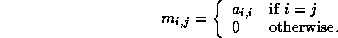
This is known as the (point) Jacobi preconditioner.
It is possible to use this preconditioner without using any extra
storage beyond that of the matrix itself. However, division operations
are usually quite costly, so in practice storage is allocated
for the reciprocals of the matrix diagonal. This strategy applies to
many preconditioners below.
Jack Dongarra
Mon Nov 20 08:52:54 EST 1995
Block Jacobi Methods
Next:
Discussion
Up:
Jacobi Preconditioning
Previous:
Jacobi Preconditioning
Block versions of the Jacobi preconditioner can be derived by a
partitioning of the variables. If the index set  is partitioned as
  with the sets
  mutually
disjoint, then
mutually
disjoint, then

The preconditioner is now a block-diagonal matrix.
Often, natural choices for the partitioning suggest themselves:
- In problems with multiple physical variables per node,
blocks can be formed by grouping the equations per node.
- In structured matrices, such as those from partial differential
equations on regular grids, a partitioning can be based on the
physical domain. Examples are a partitioning along lines in the
2D case, or planes in the 3D case. This will be discussed
further in §
.
- On parallel computers it is natural to let the
partitioning coincide with the division of variables
over the processors.
Jack Dongarra
Mon Nov 20 08:52:54 EST 1995
Discussion
Next:
SSOR preconditioning
Up:
Jacobi Preconditioning
Previous:
Block Jacobi Methods
Jacobi preconditioners need very little storage, even in the block
case, and they are easy to implement. Additionally, on parallel
computers they don't present any particular problems.
On the other hand, more sophisticated preconditioners usually yield
a larger improvement.
Jack Dongarra
Mon Nov 20 08:52:54 EST 1995
SSOR preconditioning
Next:
Incomplete Factorization Preconditioners
Up:
Preconditioners
Previous:
Discussion
The SSOR preconditioner
like the Jacobi preconditioner, can be derived from the coefficient
matrix without any work.
If the original, symmetric, matrix is decomposed as

in its diagonal, lower, and upper triangular part, the SSOR matrix is
defined as

or, parameterized by

The optimal value of the
parameter, like the
parameter in the SOR method, will reduce the number
of iterations to a lower order.
Specifically, for second order elliptic problems a spectral
condition number 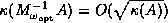 is attainable
(see Axelsson and Barker [.4]AxBa:febook). In practice,
however, the spectral
information needed to calculate the optimal
is prohibitively
expensive to compute.
is attainable
(see Axelsson and Barker [.4]AxBa:febook). In practice,
however, the spectral
information needed to calculate the optimal
is prohibitively
expensive to compute.
The SSOR matrix is given in factored form, so this preconditioner
shares many properties of other factorization-based methods (see
below). For instance, its suitability for vector processors or
parallel architectures
depends strongly on the
ordering of the variables. On the other hand, since this factorization
is given a priori, there is no possibility of breakdown as in
the construction phase of incomplete factorization methods.
Jack Dongarra
Mon Nov 20 08:52:54 EST 1995
Incomplete Factorization Preconditioners
Next:
Creating an incomplete
Up:
Preconditioners
Previous:
SSOR preconditioning
A broad class of preconditioners is based on incomplete factorizations
of the coefficient matrix. We call a factorization incomplete if
during the factorization process certain fill elements,
nonzero elements in the factorization in positions where the original
matrix had a zero, have been
ignored. Such a preconditioner is then given in factored form
with
lower and
upper triangular. The efficacy of the
preconditioner depends on how well
approximates
.
Jack Dongarra
Mon Nov 20 08:52:54 EST 1995
Introduction
Next:
Why Use Templates?
Up:
Templates for the Solution
Previous:
List of Figures
Which of the following statements is true?
- Users want ``black box''Black box: A piece of software that
can be used without knowledge of its inner workings; the user supplies the
input, and the output is more or less guaranteed to be correct.
software that they can use with
complete confidence for general problem classes without having to
understand the fine algorithmic details.
- Users want to be able to tuneTune: Adapt software
for a specific application and computing environment
in order to obtain better performance in that case only.
data structures for a particular
application, even if the software is not as reliable as that
provided for general methods.
It turns out both are true, for different groups of users.
Traditionally, users have asked for and been provided with black box
software in the form of mathematical libraries such as LAPACK
,
LINPACK
, NAG
, and
IMSL
. More recently, the
high-performance community has discovered that they must write custom
software for their problem. Their reasons include inadequate
functionality of existing software libraries, data structures that are
not natural or convenient for a particular problem, and overly general
software that sacrifices too much performance when applied to a
special case of interest.
Can we meet the needs of both groups of users? We believe we can.
Accordingly, in this book, we introduce the use of templates
Template: Description of an
algorithm, abstracting away from implementational details.
A template is a description of a general algorithm rather than the
executable object code or the source code more commonly found in a
conventional software library. Nevertheless, although templates are
general descriptions of key algorithms, they offer whatever degree of
customization the user may desire. For example, they can be
configured for the specific data structure of a problem or for the
specific computing system on which the problem is to run.
We focus on the use of iterative methods for
solving large sparse systems of linear equations.Iterative
method: An algorithm that produces a sequence of approximations to
the solution of a linear system of equations; the length of the
sequence is not given a priori by the size of the system. Usually,
the longer one iterates,
the closer one is able to get to the true solution. See: Direct method.Direct method:
An algorithm that produces the solution to a system of linear equations
in a number of operations that is determined a priori by the size
of the system. In exact arithmetic, a direct method yields the true
solution to the system. See: Iterative method.
Many methods exist for solving such
problems. The trick is to find the most effective method for the
problem at hand. Unfortunately, a method that works well for one
problem type may not work as well for another. Indeed, it may not work
at all.
Thus, besides providing templates, we suggest how to choose and
implement an effective method, and how to specialize a method to
specific matrix types. We restrict ourselves to iterative
methods, which work by repeatedly improving an approximate solution
until it is accurate enough. These methods access the coefficient
matrix
of the linear system only via the
matrix-vector product  (and
perhaps
(and
perhaps  ). Thus the user need only supply a subroutine
for computing
(and perhaps
) given
, which permits full
exploitation of the sparsity or other special structure of
.
). Thus the user need only supply a subroutine
for computing
(and perhaps
) given
, which permits full
exploitation of the sparsity or other special structure of
.
We believe that after reading this book, applications developers will
be able to use templates to get their program running on a parallel
machine quickly. Nonspecialists will know how to choose and implement
an approach to solve a particular problem. Specialists will be able
to assemble and modify their codes-without having to make the huge
investment that has, up to now, been required to tune large-scale
applications for each particular machine. Finally, we hope that all
users will gain a better understanding of the algorithms employed.
While education has not been one of the traditional goals of
mathematical software, we believe that our approach will go a long way
in providing such a valuable service.
Next:
Why Use Templates?
Up:
Templates for the Solution
Previous:
List of Figures
Jack Dongarra
Mon Nov 20 08:52:54 EST 1995
Creating an incomplete factorization
Next:
Solving a system
Up:
Incomplete Factorization Preconditioners
Previous:
Incomplete Factorization Preconditioners
Incomplete factorizations are the first preconditioners we have
encountered so far for which there is a non-trivial creation stage.
Incomplete factorizations may break down (attempted
division by zero pivot) or result in indefinite matrices (negative
pivots) even if the full factorization of the same matrix is
guaranteed to exist and yield a positive definite matrix.
An incomplete factorization is guaranteed to exist for many
factorization strategies if the original matrix is an
-matrix.
This was originally proved by Meijerink and
Van der Vorst
[152]; see
further Beauwens and Quenon
[33],
Manteuffel
[147], and
Van der Vorst
[200].
In cases where pivots are zero or negative, strategies have been
proposed such as substituting an arbitrary positive
number (see Kershaw
[132]), or restarting the factorization
on  for some positive value of
  (see
Manteuffel
[147]).
(see
Manteuffel
[147]).
An important consideration for incomplete
factorization preconditioners is the cost of the factorization process.
Even if the incomplete factorization exists,
the number of operations involved in creating it
is at least as much as for
solving a system with such a coefficient matrix, so the cost may equal
that of one
or more iterations of the iterative method. On parallel computers this
problem is aggravated by the generally poor parallel efficiency of the
factorization.
Such factorization costs can be amortized if the iterative method
takes many iterations, or if the same preconditioner will be used
for several linear systems, for instance in successive time steps or
Newton iterations.
Jack Dongarra
Mon Nov 20 08:52:54 EST 1995
Solving a system with an incomplete factorization
preconditioner
Next:
Point incomplete factorizations
Up:
Creating an incomplete
Previous:
Creating an incomplete
Incomplete factorizations can be given in various forms. If
(with
and
nonsingular triangular matrices),
solving a system proceeds in the usual way
(figure
),
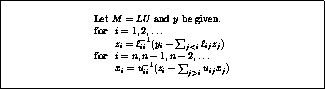
Figure: Preconditioner solve of a system  , with
but often incomplete factorizations are given as  (with
diagonal, and
and
now strictly triangular matrices, determined through
the factorization process).
In that case, one could use either of the following equivalent
formulations for
:
(with
diagonal, and
and
now strictly triangular matrices, determined through
the factorization process).
In that case, one could use either of the following equivalent
formulations for
:

or

In either case, the diagonal elements are used twice (not three times
as the formula for
would lead one to expect), and since only
divisions with
are performed, storing
explicitly is the
practical thing to do.
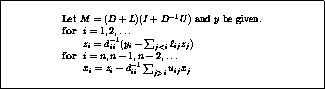
Figure: Preconditioner solve of a system
,
with  .
.
At the cost of some extra storage, one could store  or
, thereby saving some computation.
Solving a system using the first formulation is
outlined in figure
. The second formulation is
slightly harder to implement.
or
, thereby saving some computation.
Solving a system using the first formulation is
outlined in figure
. The second formulation is
slightly harder to implement.
Jack Dongarra
Mon Nov 20 08:52:54 EST 1995
Point incomplete factorizations
Next:
Fill-in strategies
Up:
Incomplete Factorization Preconditioners
Previous:
Solving a system
The most common type of incomplete factorization is based on taking a
set  of matrix positions, and keeping all positions outside this
set equal to zero during the factorization. The resulting
factorization is incomplete in the sense that fill is suppressed.
of matrix positions, and keeping all positions outside this
set equal to zero during the factorization. The resulting
factorization is incomplete in the sense that fill is suppressed.
The set
is usually chosen to encompass all positions
for
which  . A position that is zero in
but not so in an
exact factorization
is called a fill position, and if it is
outside
, the fill there is said to be ``discarded''.
Often,
is chosen to coincide with the set of nonzero positions
in
, discarding all fill. This factorization type is called
the
factorization: the Incomplete
factorization of
level zero
.
. A position that is zero in
but not so in an
exact factorization
is called a fill position, and if it is
outside
, the fill there is said to be ``discarded''.
Often,
is chosen to coincide with the set of nonzero positions
in
, discarding all fill. This factorization type is called
the
factorization: the Incomplete
factorization of
level zero
.
We can describe an incomplete factorization formally as

Meijerink and Van der Vorst
[152] proved that, if
is
an
-matrix, such a factorization exists for any choice of
, and
gives a symmetric positive definite matrix if
is symmetric
positive definite. Guidelines for allowing levels of fill were given
by Meijerink and Van der Vorst in
[153].
Jack Dongarra
Mon Nov 20 08:52:54 EST 1995
Fill-in strategies
Next:
Simple cases: and
Up:
Point incomplete factorizations
Previous:
Point incomplete factorizations
There are two major strategies for accepting or discarding fill-in,
one structural, and one numerical. The structural strategy is that of
accepting fill-in only to a certain level. As was already pointed out above,
any zero location
in
filling in (say in step
)
is assigned a fill level value

If  was already nonzero, the level value is not changed.
The numerical fill strategy is that of `drop tolerances':
fill is ignored if it is too small, for a suitable definition of
`small'. Although this definition makes more sense mathematically, it
is harder to implement in practice, since the amount of storage needed
for the factorization is not easy to predict.
See
[157]
[20] for discussions of
preconditioners using drop tolerances.
Jack Dongarra
Mon Nov 20 08:52:54 EST 1995
Simple cases: <IMG ALIGN=BOTTOM SRC="http://www.netlib.org/utk/papers/templates/_22900_tex2html_wrap6165.gif">
and <IMG ALIGN=BOTTOM SRC="http://www.netlib.org/utk/papers/templates/_22900_tex2html_wrap6389.gif">
-<IMG ALIGN=BOTTOM SRC="http://www.netlib.org/utk/papers/templates/_22900_tex2html_wrap7381.gif">
Next:
Special cases: central
Up:
Point incomplete factorizations
Previous:
Fill-in strategies
For the
method, the incomplete factorization produces no
nonzero elements beyond the sparsity structure
of the original matrix, so that the preconditioner at worst
takes exactly as much space to store as the original matrix. In a
simplified version of
, called
-
(Pommerell
[174]), even less is needed. If not only we
prohibit fill-in elements, but we also alter only the diagonal
elements (that is, any alterations of off-diagonal elements are
ignored
),
we have the following situation.
Splitting the coefficient matrix into its diagonal, lower
triangular, and upper triangular parts as
, the
preconditioner can be written as  where
is the
diagonal matrix containing the pivots generated. Generating this
preconditioner is described in figure
.
where
is the
diagonal matrix containing the pivots generated. Generating this
preconditioner is described in figure
.
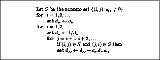
Figure: Construction of a
-
incomplete
factorization preconditioner, storing the inverses
of the pivots
Since we use the
upper and lower triangle of the matrix unchanged, only storage space
for
is needed. In fact, in order to avoid division operations
during the preconditioner solve stage we store
rather than
.
Remark: the resulting lower and upper factors of the preconditioner have
only nonzero elements in the set
, but this fact is in general not
true for the preconditioner
itself.
The fact that the
-
preconditioner contains the off-diagonal
parts of the original matrix was used by
Eisenstat
[91] to derive at a more
efficient implementation of preconditioned CG. This new
implementation merges the application of the tridiagonal factors of
the matrix and the preconditioner, thereby saving a substantial number
of operations per iteration.
Jack Dongarra
Mon Nov 20 08:52:54 EST 1995
Special cases: central differences
Next:
Modified incomplete factorizations
Up:
Point incomplete factorizations
Previous:
Simple cases: and
We will now consider the special case of
a matrix derived from central differences on a Cartesian product grid.
In this case the
and
-
factorizations coincide, and,
as remarked above, we only have to calculate the pivots of the
factorization; other elements in the triangular factors are equal to
off-diagonal elements of
.
In the following we will assume a natural, line-by-line, ordering of
the grid points.
Letting
,
be coordinates in a regular 2D grid, it is easy to see
that the pivot on grid point
is only determined by
pivots on points  and
and  . If there are
points on
each of
grid lines,
we get the following generating relations for the pivots:
. If there are
points on
each of
grid lines,
we get the following generating relations for the pivots:
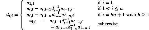
Conversely, we can describe the factorization algorithmically as

In the above we have assumed that the variables in the problem
are ordered according to the so-called ``natural ordering'': a
sequential numbering of the grid lines and the points within each grid
line. Below we will encounter different orderings of the variables.
Jack Dongarra
Mon Nov 20 08:52:54 EST 1995
Modified incomplete factorizations
Next:
Vectorization of the
Up:
Point incomplete factorizations
Previous:
Special cases: central
One modification to the basic idea of incomplete factorizations is as
follows:
If the product  is nonzero, and fill is not allowed in position
,
instead of simply discarding this fill quantity subtract it from
the diagonal element
.
Such a factorization scheme is usually called a ``modified incomplete
factorization''.
is nonzero, and fill is not allowed in position
,
instead of simply discarding this fill quantity subtract it from
the diagonal element
.
Such a factorization scheme is usually called a ``modified incomplete
factorization''.
Mathematically this corresponds to forcing the preconditioner to have
the same rowsums as the original matrix.
One reason for considering modified incomplete factorizations is the
behavior of the spectral condition number of the preconditioned
system. It was mentioned above that for second order elliptic
equations the condition number of the
coefficient matrix is  as a function of the discretization
mesh width. This order of magnitude is preserved by simple incomplete
factorizations, although usually a reduction by a large constant
factor is obtained.
as a function of the discretization
mesh width. This order of magnitude is preserved by simple incomplete
factorizations, although usually a reduction by a large constant
factor is obtained.
Modified factorizations are of interest because, in
combination with small perturbations, the spectral condition number of
the preconditioned system can be of a lower order.
It was first proved by Dupont, Kendall and
Rachford
[81] that
a modified incomplete factorization of  gives
gives
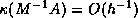 for the central difference case. More
general proofs are given by Gustafsson
[112],
Axelsson and Barker [.2]AxBa:febook, and
Beauwens
[32]
[31].
for the central difference case. More
general proofs are given by Gustafsson
[112],
Axelsson and Barker [.2]AxBa:febook, and
Beauwens
[32]
[31].
Instead of keeping row sums constant, one can also keep column
sums constant.
In computational fluid mechanics this idea is justified with the argument
that the material balance stays constant over all iterates.
(Equivalently, one wishes to avoid `artificial
diffusion'.)
Appleyard and Cheshire
[4] observed that if
and
have the same column sums, the choice

guarantees
that the sum of the elements in  (the material balance error) is
zero, and that all further
(the material balance error) is
zero, and that all further  have elements summing to zero.
Modified incomplete factorizations can break down,
especially when the variables are numbered other than in the natural
row-by-row ordering. This was noted by Chan and
Kuo
[50], and a full analysis was given by
Eijkhout
[86] and Notay
[161].
A slight variant of modified incomplete factorizations consists of the
class of ``relaxed incomplete factorizations''. Here the fill is
multiplied by a parameter  before it is subtracted from
the diagonal; see
Ashcraft and Grimes
[11],
Axelsson and Lindskog
[19]
[18],
Chan
[44],
Eijkhout
[86],
Notay
[162],
Stone
[194], and
Van der Vorst
[204].
For the dangers of MILU in the presence of rounding error, see
Van der Vorst
[206].
before it is subtracted from
the diagonal; see
Ashcraft and Grimes
[11],
Axelsson and Lindskog
[19]
[18],
Chan
[44],
Eijkhout
[86],
Notay
[162],
Stone
[194], and
Van der Vorst
[204].
For the dangers of MILU in the presence of rounding error, see
Van der Vorst
[206].
Next:
Vectorization of the
Up:
Point incomplete factorizations
Previous:
Special cases: central
Jack Dongarra
Mon Nov 20 08:52:54 EST 1995
Vectorization of the preconditioner solve
Next:
Parallelizing the preconditioner
Up:
Point incomplete factorizations
Previous:
Modified incomplete factorizations
At first it may appear that the sequential time of solving a
factorization is of the order of the number of variables, but things
are not quite that bad. Consider the special case of central
differences on a regular domain of
points. The variables
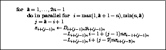
Figure: Wavefront solution of  from a central difference problem
on a domain of
from a central difference problem
on a domain of  points.
on any diagonal in the domain, that is,
in locations
with  , depend
only on those on the previous diagonal, that is, with
, depend
only on those on the previous diagonal, that is, with  .
Therefore it is possible to process the operations on such a diagonal,
or `wavefront'
,
in parallel (see figure
),
or have a vector computer pipeline them;
see Van der Vorst
[205]
[203].
.
Therefore it is possible to process the operations on such a diagonal,
or `wavefront'
,
in parallel (see figure
),
or have a vector computer pipeline them;
see Van der Vorst
[205]
[203].
Another way of vectorizing the solution of the triangular factors is
to use some form of expansion of the inverses of the factors.
Consider for a moment a lower triangular matrix, normalized to
the form  where
is strictly lower triangular). Its
inverse can be given as either of the following two series:
where
is strictly lower triangular). Its
inverse can be given as either of the following two series:

(The first series is called a ``Neumann expansion'', the second an
``Euler expansion''. Both series are finite, but their length
prohibits practical use of this fact.)
Parallel or vectorizable preconditioners can be derived from an
incomplete factorization by taking a small number of terms in either
series.
Experiments indicate that a small number of terms, while
giving high execution rates, yields almost the full precision of the
more recursive triangular solution (see
Axelsson and Eijkhout
[15] and
Van der Vorst
[201]).
There are some practical considerations in implementing these
expansion algorithms. For instance, because of the normalization the
in equation (
) is not  . Rather, if we
have a preconditioner (as described in section
)
described by
. Rather, if we
have a preconditioner (as described in section
)
described by

then we write

Now we can choose whether or not to store the product  .
Doing so doubles the storage requirements for the matrix, not doing so
means that separate multiplications by
and
have to be
performed in the expansion.
.
Doing so doubles the storage requirements for the matrix, not doing so
means that separate multiplications by
and
have to be
performed in the expansion.
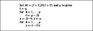
Figure: Preconditioning step algorithm for
a Neumann expansion  of an incomplete factorization
 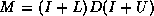 .
.
Suppose then that the products  and
and  have been
stored. We then define
by
have been
stored. We then define
by

and replace solving a system
for
by computing  .
This algorithm is given in figure
.
.
This algorithm is given in figure
.
Next:
Parallelizing the preconditioner
Up:
Point incomplete factorizations
Previous:
Modified incomplete factorizations
Jack Dongarra
Mon Nov 20 08:52:54 EST 1995
Parallelizing the preconditioner solve
Next:
Block factorization methods
Up:
Point incomplete factorizations
Previous:
Vectorization of the
The algorithms for vectorization outlined above can be used on
parallel computers. For instance, variables on a wavefront
can be
processed in parallel, by dividing the wavefront over processors.
More radical approaches for increasing the parallelism in incomplete
factorizations are based on a renumbering of the problem variables.
For instance, on rectangular domains one could start numbering the
variables from all four corners simultaneously, thereby creating
four simultaneous wavefronts, and therefore four-fold parallelism
(see Dongarra, et al.
[71],
Van der Vorst
[204]
[202])
.
The most extreme case is the red/black ordering
(or for more general matrices the multi-color ordering) which gives
the absolute minimum number of sequential steps.
Multi-coloring is also an attractive method for vector computers.
Since points of one color are uncoupled, they can be processed as one
vector; see Doi
[68],
Melhem
[154], and Poole and
Ortega
[176].
However, for such ordering strategies there is usually a trade-off
between the degree of parallelism and the resulting number of
iterations. The reason for this is that a different ordering may give
rise to a different error matrix, in particular the norm of the error
matrix may vary considerably between orderings.
See experimental results by Duff and Meurant
[79] and a
partial explanation of them by Eijkhout
[85].
Jack Dongarra
Mon Nov 20 08:52:54 EST 1995
Block factorization methods
Next:
The idea behind
Up:
Incomplete Factorization Preconditioners
Previous:
Parallelizing the preconditioner
We can also consider block variants of preconditioners for accelerated
methods. Block methods are normally feasible if the problem domain is
a Cartesian product grid; in that case a natural division in lines (or
planes in the 3-dimensional case), can be used for blocking, though
incomplete factorizations are not as effective in the 3-dimensional
case; see for instance Kettler
[134].
In such a blocking scheme for Cartesian product grids,
both the size and number of the
blocks increases with the overall problem size.
Jack Dongarra
Mon Nov 20 08:52:54 EST 1995
Why Use Templates?
Next:
What Methods Are
Up:
Introduction
Previous:
Introduction
Templates offer three significant advantages. First, templates are
general and reusable. Thus, they can simplify ports to diverse
machines. This feature is important given the diversity
of parallel architectures.
Second, templates exploit the expertise of two distinct groups. The
expert numerical analyst creates a template reflecting in-depth
knowledge of a specific numerical technique. The computational scientist
then provides ``value-added'' capability to the general template
description, customizing it for specific contexts or applications
needs.
And third, templates are not language specific. Rather, they are
displayed in an Algol-like structure, which is readily translatable
into the target language such as FORTRAN (with the use of the
Basic Linear Algebra Subprograms, or BLAS
,
whenever possible) and C. By using these familiar styles, we
believe that the users will have trust in the algorithms. We also
hope that users will gain a better understanding of numerical
techniques and parallel programming.
For each template, we provide some or all of the following:
- a mathematical description of the flow of the iteration;
- discussion of convergence and stopping criteria;
- suggestions for applying a method to special matrix types
(e.g., banded systems);
- advice for tuning (for example, which preconditioners are
applicable and which are not);
- tips on parallel implementations; and
- hints as to when to use a method, and why.
For each of the templates, the following can be obtained via electronic mail.
- a MATLAB
implementation based on
dense matrices;
- a FORTRAN-77
program with calls to
BLAS
;
- a C++
template implementation for matrix/vector classes.
See Appendix
for details.
Jack Dongarra
Mon Nov 20 08:52:54 EST 1995
The idea behind block factorizations
Next:
Approximate inverses
Up:
Block factorization methods
Previous:
Block factorization methods
The starting point for an incomplete block factorization is a
partitioning of the matrix, as mentioned in §
.
Then an incomplete factorization is performed using the matrix blocks
as basic entities (see Axelsson
[12] and Concus, Golub
and Meurant
[57] as
basic references).
The most important difference with point methods arises in the
inversion of the pivot blocks. Whereas inverting a scalar is easily
done, in the block case two problems arise. First, inverting
the pivot block is likely to be a costly operation. Second, initially the
diagonal blocks of the matrix are likely to be be sparse
and we would like to maintain this type of
structure throughout the factorization.
Hence the need for approximations of inverses arises.
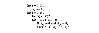
Figure: Block version of a
-
factorization
In addition to this, often fill-in in off-diagonal blocks is discarded
altogether. Figure
describes an incomplete block
factorization that is analogous to the
-
factorization
(section
) in that it only updates the diagonal blocks.
As in the case of incomplete point factorizations, the existence of
incomplete block methods is guaranteed if the coefficient
matrix is an
-matrix. For a general proof, see
Axelsson
[13].
Jack Dongarra
Mon Nov 20 08:52:54 EST 1995
Approximate inverses
Next:
The special case
Up:
Block factorization methods
Previous:
The idea behind
In block factorizations a pivot block is generally forced to be
sparse, typically of banded form, and that we need an approximation to
its inverse that has a similar structure. Furthermore, this
approximation should be easily computable, so we rule out the option
of calculating the full inverse and taking a banded part of it.
The simplest approximation to
is the diagonal matrix
of
the reciprocals of the diagonal of
:  .
.
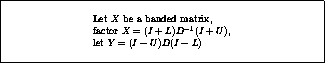
Figure: Algorithm for approximating the inverse of a banded matrix
Other possibilities were considered by
Axelsson and Eijkhout
[15],
Axelsson and Polman
[21],
Concus, Golub and Meurant
[57],
Eijkhout and Vassilevski
[90],
Kolotilina and Yeremin
[141],
and Meurant
[155]. One particular
example is given in figure
. It has the attractive
theoretical property that, if the original matrix is symmetric
positive definite and a factorization with positive diagonal
can
be made, the approximation to the inverse is again symmetric positive
definite.
Banded approximations to the inverse of banded matrices have a
theoretical justification. In the context of partial differential
equations the diagonal blocks of the coefficient matrix are usually
strongly diagonally dominant. For such matrices, the elements of the
inverse have a size that is exponentially decreasing in their distance
from the main diagonal. See Demko, Moss and
Smith
[65] for a general
proof, and Eijkhout and Polman
[89] for a more detailed
analysis in the
-matrix case.
Jack Dongarra
Mon Nov 20 08:52:54 EST 1995
The special case of block tridiagonality
Next:
Two types of
Up:
Block factorization methods
Previous:
Approximate inverses
In many applications, a block tridiagonal structure can be found in
the coefficient matrix. Examples are problems on a 2D regular grid if
the blocks correspond to lines of grid points, and problems on a
regular 3D grid, if the blocks correspond to planes of grid points.
Even if such a block tridiagonal structure does not arise naturally,
it can be imposed by renumbering the variables in a Cuthill-McKee
ordering
[60].
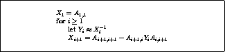
Figure: Incomplete block factorization of a block tridiagonal matrix
Such a matrix has incomplete block factorizations of a particularly
simple nature: since no fill can occur outside the diagonal
blocks  ,
all properties follow from our treatment of the pivot blocks. The
generating recurrence for the pivot blocks also takes a simple form,
see figure
. After the factorization we are left
with sequences of
,
all properties follow from our treatment of the pivot blocks. The
generating recurrence for the pivot blocks also takes a simple form,
see figure
. After the factorization we are left
with sequences of  block forming the pivots, and of
  blocks
approximating their inverses.
blocks
approximating their inverses.
Jack Dongarra
Mon Nov 20 08:52:54 EST 1995
Two types of incomplete block factorizations
Next:
Blocking over systems
Up:
Block factorization methods
Previous:
The special case
One reason that block methods are of interest is that they are
potentially more suitable for vector computers and parallel
architectures. Consider the block factorization

where
is the block diagonal matrix of pivot blocks,
and
,
are the block lower and upper triangle of the factorization;
they coincide with
,  in the case of a block tridiagonal
matrix.
in the case of a block tridiagonal
matrix.
We can turn this into an incomplete factorization by replacing the
block diagonal matrix of pivots
by the block diagonal matrix of
incomplete factorization pivots  , giving

For factorizations of this type (which covers all
methods in Concus, Golub and Meurant
[57] and
Kolotilina and Yeremin
[141]) solving
a linear system means solving
smaller systems with the
matrices.
Alternatively, we can replace
by a
the inverse of the block diagonal matrix of the
approximations to the inverses of the pivots,  , giving

For this second type (which
was discussed by Meurant
[155], Axelsson and
Polman
[21] and Axelsson and
Eijkhout
[15]) solving
a system with
entails multiplying by the
blocks.
Therefore, the second type has a much higher potential for
vectorizability. Unfortunately, such a factorization is theoretically
more troublesome; see the above references or Eijkhout and
Vassilevski
[90].
Jack Dongarra
Mon Nov 20 08:52:54 EST 1995
Blocking over systems of partial differential
equations
Next:
Incomplete LQ factorizations
Up:
Incomplete Factorization Preconditioners
Previous:
Two types of
If the physical problem has several variables per grid point, that is,
if there are several coupled partial differential equations, it is
possible to introduce blocking in a natural way.
Blocking of the equations (which gives a small number of very large
blocks) was used by Axelsson and Gustafsson
[17] for
the equations of linear
elasticity, and blocking of the
variables per node (which gives many very small blocks) was used
by Aarden and Karlsson
[1] for the
semiconductor
equations. A systematic comparison of the two approaches was made
by Bank, et al.
[26].
Jack Dongarra
Mon Nov 20 08:52:54 EST 1995
Incomplete LQ factorizations
Next:
Polynomial preconditioners
Up:
Incomplete Factorization Preconditioners
Previous:
Blocking over systems
Saad
[184] proposes to construct an incomplete LQ factorization
of a general sparse matrix. The idea is to orthogonalize the rows
of the matrix by a Gram-Schmidt process (note that in sparse matrices,
most rows are typically orthogonal already, so that standard Gram-Schmidt
may be not so bad as in general). Saad suggest dropping strategies for
the fill-in produced in the orthogonalization process. It turns out that
the resulting incomplete L factor can be viewed as the incomplete Cholesky
factor of the matrix
. Experiments show that using
in a CG
process for the normal equations: 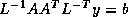 is effective for
some relevant problems.
is effective for
some relevant problems.
Jack Dongarra
Mon Nov 20 08:52:54 EST 1995
Polynomial preconditioners
Next:
Preconditioners from properties
Up:
Preconditioners
Previous:
Incomplete LQ factorizations
So far, we have described preconditioners in only one of two classes:
those that approximate the coefficient
matrix, and where linear systems with the preconditioner as
coefficient matrix are easier to solve than the original system.
Polynomial preconditioners can be considered as members of the
second class of preconditioners:
direct approximations of the inverse of the coefficient matrix.
Suppose that the coefficient matrix
of the linear system is
normalized to
the form  , and that the spectral radius of
is less than
one. Using the Neumann series, we can write the inverse of
as
, and that the spectral radius of
is less than
one. Using the Neumann series, we can write the inverse of
as
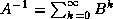 ,
so an approximation may be derived by truncating this infinite series.
Since the iterative methods we are considering are already based on
the idea of applying polynomials in the coefficient matrix to the
initial residual, there are analytic connections between the basic
method and polynomially accelerated one.
,
so an approximation may be derived by truncating this infinite series.
Since the iterative methods we are considering are already based on
the idea of applying polynomials in the coefficient matrix to the
initial residual, there are analytic connections between the basic
method and polynomially accelerated one.
Dubois, Greenbaum and Rodrigue
[77]
investigated the relationship between a basic method
using a splitting  , and a polynomially preconditioned method
with
, and a polynomially preconditioned method
with
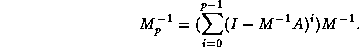
The basic result is that for classical methods,
steps of the polynomially preconditioned method are
exactly equivalent to
 steps of the original method; for accelerated
methods, specifically the Chebyshev method, the preconditioned
iteration can improve the number of iterations by at most a factor
of
.
steps of the original method; for accelerated
methods, specifically the Chebyshev method, the preconditioned
iteration can improve the number of iterations by at most a factor
of
.
Although there is no gain in the number of times the coefficient
matrix is applied, polynomial preconditioning does eliminate a large
fraction of the inner
products and update operations, so there may be an overall increase in
efficiency.
Let us define a polynomial preconditioner more abstractly as any
polynomial  normalized to
  . Now the choice of the
best polynomial preconditioner becomes that of choosing the best
polynomial that minimizes
. Now the choice of the
best polynomial preconditioner becomes that of choosing the best
polynomial that minimizes  . For the choice of the
infinity norm we thus obtain Chebyshev polynomials, and they require
estimates of both a lower and upper bound on the spectrum of
.
These estimates may be derived from the conjugate gradient iteration
itself; see §
.
. For the choice of the
infinity norm we thus obtain Chebyshev polynomials, and they require
estimates of both a lower and upper bound on the spectrum of
.
These estimates may be derived from the conjugate gradient iteration
itself; see §
.
Since an accurate lower bound on the spectrum of
may be hard to
obtain, Johnson, Micchelli and Paul
[126]
and Saad
[183] propose least
squares polynomials based on several weight functions.
These functions only require an upper bound and this is easily
computed, using for instance the ``Gerschgorin bound''
 ; see [.4]Va:book.
Experiments comparing Chebyshev and least squares polynomials can be
found in Ashby, Manteuffel and Otto
[8].
; see [.4]Va:book.
Experiments comparing Chebyshev and least squares polynomials can be
found in Ashby, Manteuffel and Otto
[8].
Application of polynomial preconditioning to symmetric indefinite
problems is described by Ashby, Manteuffel and
Saylor
[9]. There the
polynomial is chosen so that it transforms the system into a
definite one.
Next:
Preconditioners from properties
Up:
Preconditioners
Previous:
Incomplete LQ factorizations
Jack Dongarra
Mon Nov 20 08:52:54 EST 1995
Preconditioners from properties of the
differential equation
Next:
Preconditioning by the
Up:
Preconditioners
Previous:
Polynomial preconditioners
A number of preconditioners exist that derive their justification from
properties of the underlying partial differential equation. We will
cover some of them here (see also §
and §
). These preconditioners usually involve more
work than the types discussed above, however, they allow for
specialized faster solution methods.
Jack Dongarra
Mon Nov 20 08:52:54 EST 1995
Preconditioning by the symmetric part
Next:
The use of
Up:
Preconditioners from properties
Previous:
Preconditioners from properties
In §
we pointed out that conjugate
gradient methods for non-selfadjoint systems require the storage of
previously calculated vectors. Therefore it is somewhat remarkable
that preconditioning by the symmetric part  of the coefficient matrix
leads to a method that does not need this extended storage.
Such a method was proposed by Concus and Golub
[56]
and Widlund
[216].
of the coefficient matrix
leads to a method that does not need this extended storage.
Such a method was proposed by Concus and Golub
[56]
and Widlund
[216].
However, solving a system with the symmetric part of a matrix may be
no easier than solving a system with the full matrix. This problem may
be tackled by imposing a nested iterative method, where a
preconditioner based on the symmetric part is used.
Vassilevski
[212] proved that the efficiency of this
preconditioner for the symmetric part carries over to the outer
method.
Jack Dongarra
Mon Nov 20 08:52:54 EST 1995
The use of fast solvers
Next:
Alternating Direction Implicit
Up:
Preconditioners from properties
Previous:
Preconditioning by the
In many applications, the coefficient matrix is symmetric and positive
definite. The reason for this is usually that the partial differential
operator from which it is derived is self-adjoint, coercive, and bounded
(see Axelsson and Barker [.2]AxBa:febook).
It follows that for the coefficient
matrix
the following relation holds for any matrix
from a
similar differential equation:
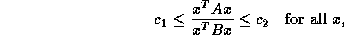
where  ,
,  do not depend on the matrix size. The importance of
this is that the use of
as a preconditioner gives an iterative
method with a number of iterations that does not depend on the matrix size.
do not depend on the matrix size. The importance of
this is that the use of
as a preconditioner gives an iterative
method with a number of iterations that does not depend on the matrix size.
Thus we can precondition our original matrix by one derived from a
different PDE, if one can be found that has attractive properties as
preconditioner.
The most common choice is to take a matrix from a separable PDE. A system involving such a matrix can be solved with
various so-called ``fast solvers'', such as FFT methods, cyclic
reduction, or the generalized marching algorithm
(see Dorr
[75],
Swarztrauber
[195], Bank
[25] and
Bank and Rose
[27]).
As a simplest example, any elliptic operator can be preconditioned
with the Poisson operator, giving the iterative method

In Concus and Golub
[59] a transformation of this
method is considered to speed up the convergence.
As another example, if the original matrix arises from

the preconditioner can be formed from

An extension to the non-self adjoint case is considered
by Elman and Schultz
[94].
Fast solvers are attractive in that the number of operations they
require is (slightly higher than) of the order of the number of
variables. Coupled with the fact that the number of iterations in the
resulting preconditioned iterative methods is independent of the
matrix size, such methods are close to optimal. However, fast solvers
are usually only applicable if the physical domain is a rectangle or
other Cartesian product structure. (For a domain consisting of a
number of such pieces, domain decomposition methods can be used;
see §
).
Next:
Alternating Direction Implicit
Up:
Preconditioners from properties
Previous:
Preconditioning by the
Jack Dongarra
Mon Nov 20 08:52:54 EST 1995
What Methods Are Covered?
Next:
Iterative Methods
Up:
Introduction
Previous:
Why Use Templates?
Many iterative methods have been developed and it is impossible to
cover them all. We chose the methods below either because they
illustrate the historical development of iterative methods, or because
they represent the current state-of-the-art for solving large sparse
linear systems. The methods we discuss are:
- Jacobi
- Gauss-Seidel
- Successive Over-Relaxation (SOR
)
- Symmetric Successive Over-Relaxation (SSOR
)
- Conjugate Gradient (CG
)
- Minimal Residual (MINRES
)
and Symmetric LQ (SYMMLQ
)
- Conjugate Gradients on the Normal Equations
(CGNE
and CGNR
)
- Generalized Minimal Residual (GMRES
)
- Biconjugate Gradient (BiCG
)
- Quasi-Minimal Residual (QMR
)
- Conjugate Gradient Squared (CGS
)
- Biconjugate Gradient Stabilized (Bi-CGSTAB
)
- Chebyshev
Iteration
For each method we present a general description, including a
discussion of the history of the method and numerous references to the
literature. We also give the mathematical conditions for selecting a
given method.
We do not intend to write a ``cookbook'', and have deliberately
avoided the words ``numerical recipes'', because these phrases imply
that our algorithms can be used blindly without knowledge of the
system of equations. The state of the art in iterative methods does
not permit this: some knowledge about the linear system is needed to
guarantee convergence of these algorithms, and generally the more that
is known the more the algorithm can be tuned. Thus, we have chosen to
present an algorithmic outline, with guidelines for choosing a method
and implementing it on particular kinds of high-performance machines.
We also discuss the use of preconditioners and relevant data storage
issues.
Jack Dongarra
Mon Nov 20 08:52:54 EST 1995
Alternating Direction Implicit methods
Next:
Related Issues
Up:
Preconditioners from properties
Previous:
The use of
The Poisson differential operator can be split in a natural way
as the sum of two operators:

Now let  ,
,  be discretized representations of
  ,
,  . Based on the observation that
 , iterative schemes
such as
, iterative schemes
such as

with suitable choices of  and
and  have been proposed.
This alternating direction implicit, or ADI, method was first
proposed as a solution method for parabolic equations. The  are then approximations on subsequent time steps. However, it can also
be used for the steady state, that is, for solving elliptic equations.
In that case, the
become subsequent iterates;
see D'Yakonov
[82],
Fairweather, Gourlay and Mitchell
[97],
Hadjidimos
[119], and
Peaceman and Rachford
[173].
Generalization
of this scheme to variable coefficients or fourth order elliptic
problems is relatively straightforward.
are then approximations on subsequent time steps. However, it can also
be used for the steady state, that is, for solving elliptic equations.
In that case, the
become subsequent iterates;
see D'Yakonov
[82],
Fairweather, Gourlay and Mitchell
[97],
Hadjidimos
[119], and
Peaceman and Rachford
[173].
Generalization
of this scheme to variable coefficients or fourth order elliptic
problems is relatively straightforward.
The above method is implicit since it requires systems solutions, and it
alternates the
and
(and if necessary
) directions. It is
attractive from a practical point of view (although mostly on tensor
product grids), since solving a system with, for instance,
a matrix  entails only a number of uncoupled tridiagonal
solutions. These need very little storage over that needed for the
matrix, and they can be executed in parallel
, or one can vectorize
over them.
entails only a number of uncoupled tridiagonal
solutions. These need very little storage over that needed for the
matrix, and they can be executed in parallel
, or one can vectorize
over them.
A theoretical reason that ADI preconditioners are of interest is that
they can be shown to be
spectrally equivalent to the original coefficient matrix. Hence the
number of iterations is bounded independent of the condition number.
However, there is a problem of data distribution. For vector
computers, either the system solution with
or with
will
involve very large strides: if columns of variables in the grid are
stored contiguously, only the solution with
will involve
contiguous data. For the
the stride equals the number of
variables in a column.
On parallel machines an efficient solution is possible if the
processors are arranged in a  grid. During, e.g., the
solve, every processor row then works independently of other
rows. Inside each row, the processors can work together, for instance
using a Schur complement method. With sufficient network bandwidth
this will essentially reduce the time
to that for solving any of the subdomain
systems plus the time for the interface system. Thus, this method will
be close to optimal.
grid. During, e.g., the
solve, every processor row then works independently of other
rows. Inside each row, the processors can work together, for instance
using a Schur complement method. With sufficient network bandwidth
this will essentially reduce the time
to that for solving any of the subdomain
systems plus the time for the interface system. Thus, this method will
be close to optimal.
Next:
Related Issues
Up:
Preconditioners from properties
Previous:
The use of
Jack Dongarra
Mon Nov 20 08:52:54 EST 1995
Related Issues
Next:
Complex Systems
Up:
Templates for the Solution
Previous:
Alternating Direction Implicit
Jack Dongarra
Mon Nov 20 08:52:54 EST 1995
Complex Systems
Next:
Stopping Criteria
Up:
Related Issues
Previous:
Related Issues
Conjugate gradient methods for real symmetric systems can be applied
to complex Hermitian systems in a straightforward manner. For
non-Hermitian complex systems we distinguish two cases. In general,
for any coefficient matrix a CGNE method is possible,
that is, a conjugate gradients method on the normal equations
 ,
or one can split the system into real and complex parts and use
a method such as GMRES on the resulting real nonsymmetric system.
However, in certain practical situations the complex system is
non-Hermitian but symmetric.
,
or one can split the system into real and complex parts and use
a method such as GMRES on the resulting real nonsymmetric system.
However, in certain practical situations the complex system is
non-Hermitian but symmetric.
Complex symmetric systems can be solved by a classical conjugate
gradient or Lanczos method, that is, with short recurrences, if the
complex inner product  is replaced by
  .
Like the BiConjugate Gradient method, this method is susceptible to
breakdown, that is, it can happen that
.
Like the BiConjugate Gradient method, this method is susceptible to
breakdown, that is, it can happen that  for
for  .
A look-ahead strategy can remedy this in most
cases (see Freund
[100]
and Van der Vorst and Melissen
[208]).
.
A look-ahead strategy can remedy this in most
cases (see Freund
[100]
and Van der Vorst and Melissen
[208]).
Jack Dongarra
Mon Nov 20 08:52:54 EST 1995
Stopping Criteria
Next:
More Details about
Up:
Related Issues
Previous:
Complex Systems
Stopping criterion: Since an iterative method computes successive
approximations to the solution of a linear system, a practical test is needed
to determine when to stop the iteration. Ideally this test would measure
the distance of the last iterate to the true solution, but this is not
possible. Instead, various other metrics are used, typically involving
the residual.
Forward error: The difference between a computed iterate and
the true solution of a linear system, measured in some vector norm.
Backward error: The size of perturbations
of
the coefficient matrix and
of the right hand side
of a linear system, such that the computed iterate
is the
solution of
.
An iterative method produces a sequence  of vectors
converging to the vector
satisfying the
system
.
To be effective, a method must decide when to stop. A good stopping
criterion should
of vectors
converging to the vector
satisfying the
system
.
To be effective, a method must decide when to stop. A good stopping
criterion should
- identify when the error
 is small
enough to stop,
is small
enough to stop,
- stop if the error is no longer decreasing or decreasing too slowly, and
- limit the maximum amount of time spent iterating.
For the user wishing to read as little as possible,
the following simple stopping criterion will likely be adequate.
The user must supply the quantities
 ,
,  , stop_tol, and preferably also
  :
:
- The integer
is the maximum number of iterations the algorithm
will be permitted to perform.
- The real number
is a norm of
. Any reasonable
(order of magnitude) approximation of the absolute value of
the largest entry of the matrix
will do.
- The real number
is a norm of
. Again, any
reasonable approximation of the
absolute value of the largest entry of
will do.
- The real number stop_tol measures how small the user wants
the residual
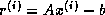 of the ultimate solution
to be. One way to choose stop_tol is as the
approximate uncertainty in the entries of
and
relative to
and
, respectively. For example, choosing stop_tol
of the ultimate solution
to be. One way to choose stop_tol is as the
approximate uncertainty in the entries of
and
relative to
and
, respectively. For example, choosing stop_tol
 means that the user considers the entries of
and
to have errors in the range
means that the user considers the entries of
and
to have errors in the range  and
and  , respectively. The algorithm will compute
no more
accurately than its inherent uncertainty warrants. The user should
choose stop_tol less than one and greater than the machine
precision
, respectively. The algorithm will compute
no more
accurately than its inherent uncertainty warrants. The user should
choose stop_tol less than one and greater than the machine
precision  .
.
Here is the algorithm:
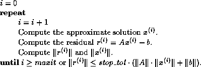
Note that if
does not change much from step to step, which occurs
near convergence, then  need not be recomputed.
If
is not available, the stopping criterion may be replaced with
the generally stricter criterion
need not be recomputed.
If
is not available, the stopping criterion may be replaced with
the generally stricter criterion

In either case, the final error bound is
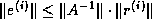 .
If an estimate of
.
If an estimate of  is available, one may also use the stopping
criterion
is available, one may also use the stopping
criterion

which guarantees that the relative error  in the computed solution is bounded by stop_tol.
Next:
More Details about
Up:
Related Issues
Previous:
Complex Systems
Jack Dongarra
Mon Nov 20 08:52:54 EST 1995
More Details about Stopping Criteria
Next:
When or is
Up:
Stopping Criteria
Previous:
Stopping Criteria
Ideally we would like to stop when the magnitudes of entries of the error
 fall below a user-supplied threshold.
But
fall below a user-supplied threshold.
But  is hard to estimate directly, so
we use the residual
instead, which is
more readily computed. The rest of this section describes how to measure
the sizes of vectors
and
, and how to bound
in terms of
.
is hard to estimate directly, so
we use the residual
instead, which is
more readily computed. The rest of this section describes how to measure
the sizes of vectors
and
, and how to bound
in terms of
.
We will measure errors using vector and matrix norms.
The most common vector norms are:
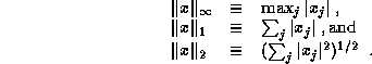
For some algorithms we may also use the norm
 , where
is a fixed nonsingular
matrix and
, where
is a fixed nonsingular
matrix and  is one of
  ,
, or
.
Corresponding to these vector norms are three matrix norms:
,
, or
.
Corresponding to these vector norms are three matrix norms:
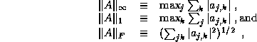
as well as  .
We may also use the matrix norm
.
We may also use the matrix norm
 , where
denotes the largest eigenvalue.
Henceforth
, where
denotes the largest eigenvalue.
Henceforth  and
will refer to any mutually
consistent pair of the above.
(
and
will refer to any mutually
consistent pair of the above.
( and
and  , as well as
and
, as well as
and  , both form
mutually consistent pairs.)
All these norms satisfy the triangle inequality
, both form
mutually consistent pairs.)
All these norms satisfy the triangle inequality  and
and  , as well as
  for mutually consistent pairs.
(For more details on the properties of norms, see Golub and
Van Loan
[109].)
for mutually consistent pairs.
(For more details on the properties of norms, see Golub and
Van Loan
[109].)
One difference between these norms is their dependence on dimension.
A vector
of length
with entries uniformly distributed between
0 and 1 will satisfy  , but
will grow
like
, but
will grow
like  and
and  will grow like
. Therefore a stopping
criterion based on
(or
) may have to be permitted to
grow proportional to
(or
) in order that it does not become
much harder to satisfy for large
.
will grow like
. Therefore a stopping
criterion based on
(or
) may have to be permitted to
grow proportional to
(or
) in order that it does not become
much harder to satisfy for large
.
There are two approaches to bounding the
inaccuracy of the computed solution to
.
Since  ,
which we will call the forward error,
is hard to estimate directly,
we introduce
the backward error, which allows us to bound the forward error.
The normwise backward error is defined as
the smallest possible value of
,
which we will call the forward error,
is hard to estimate directly,
we introduce
the backward error, which allows us to bound the forward error.
The normwise backward error is defined as
the smallest possible value of
 where
is the exact solution of
where
is the exact solution of 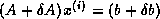 (here
denotes a general matrix, not
times
; the
same goes for
).
The backward error may be easily computed from the residual
; we show how below.
Provided one has
some bound on the inverse of
,
one can bound the forward error in terms of the backward error via
the simple equality
(here
denotes a general matrix, not
times
; the
same goes for
).
The backward error may be easily computed from the residual
; we show how below.
Provided one has
some bound on the inverse of
,
one can bound the forward error in terms of the backward error via
the simple equality

which implies
.
Therefore, a stopping criterion of the form ``stop when  '' also yields an upper bound on the forward error
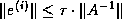 . (Sometimes we may prefer to
use the stricter but harder to estimate bound
. (Sometimes we may prefer to
use the stricter but harder to estimate bound  ; see §
. Here
; see §
. Here
 is the matrix or vector of absolute values of components of
 .)
.)
The backward error also has a direct interpretation as a stopping
criterion, in addition to supplying a bound on the forward error.
Recall that the backward error is the smallest change
to the problem
that makes
an exact solution of
. If the original data
and
have
errors from previous computations or measurements,
then it is usually not worth iterating until
and
are even
smaller than these errors.
For example, if the machine precision is
, it is not
worth making  and
and
 , because just rounding the entries
of
and
to fit in the machine creates errors this large.
, because just rounding the entries
of
and
to fit in the machine creates errors this large.
Based on this discussion, we will now consider
some stopping criteria and their
properties. Above we already mentioned
- Criterion 1.
-
 .
This is equivalent to asking that
the backward error
and
described above satisfy
.
This is equivalent to asking that
the backward error
and
described above satisfy
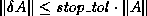 and
and
 .
This criterion yields the forward error bound
.
This criterion yields the forward error bound

The second stopping criterion we discussed, which does not require
,
may be much more stringent than Criterion 1:
- Criterion 2.
-
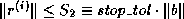 .
This is equivalent to asking that
the backward error
and
satisfy
.
This is equivalent to asking that
the backward error
and
satisfy
 and
and  .
One difficulty with this method is that if
.
One difficulty with this method is that if  ,
which can only occur if
is very ill-conditioned and
nearly
lies in the null space of
,
then it may be difficult
for any method to satisfy the stopping criterion. To see that
must
be very ill-conditioned, note that
,
which can only occur if
is very ill-conditioned and
nearly
lies in the null space of
,
then it may be difficult
for any method to satisfy the stopping criterion. To see that
must
be very ill-conditioned, note that
This criterion yields the forward error bound

If an estimate of
is available, one can also just stop
when the upper bound on the error  falls below
a threshold. This yields the third stopping criterion:
falls below
a threshold. This yields the third stopping criterion:
- Criterion 3.
-
 .
This stopping criterion guarantees that
.
This stopping criterion guarantees that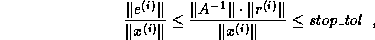
permitting the user to specify the desired relative accuracy stop_tol
in the computed solution
.
One drawback to Criteria 1 and 2 is that they usually treat backward errors in
each component of
and
equally, since most
norms  and
and  measure each entry of
and
equally.
For example, if
is sparse and
is dense, this loss of
possibly important structure will not be reflected in
.
In contrast, the following stopping criterion gives one the option of scaling
each component
measure each entry of
and
equally.
For example, if
is sparse and
is dense, this loss of
possibly important structure will not be reflected in
.
In contrast, the following stopping criterion gives one the option of scaling
each component  and
and  differently,
including the possibility of insisting that some entries be zero.
The cost is an extra matrix-vector multiply:
differently,
including the possibility of insisting that some entries be zero.
The cost is an extra matrix-vector multiply:
- Criterion 4.
-
 .
Here
.
Here  is a user-defined matrix of nonnegative entries,
is a user-defined vector of nonnegative entries, and
is a user-defined matrix of nonnegative entries,
is a user-defined vector of nonnegative entries, and
 denotes the vector of absolute values of the entries of
.
If this criterion is satisfied, it means there are a
and a
such that
, with
denotes the vector of absolute values of the entries of
.
If this criterion is satisfied, it means there are a
and a
such that
, with
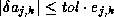 , and
, and
 for all
and
.
By choosing
and
, the user can vary the way
the backward error is measured
in the stopping criterion. For example, choosing
for all
and
.
By choosing
and
, the user can vary the way
the backward error is measured
in the stopping criterion. For example, choosing  and
and  makes the stopping criterion
 ,
which is essentially the same as Criterion 1. Choosing
,
which is essentially the same as Criterion 1. Choosing  and
and
 makes the stopping criterion measure the
componentwise relative backward error, i.e., the smallest relative
perturbations in any component of
and
which is necessary to make
an exact solution. This tighter stopping criterion requires, among other
things, that
have the same sparsity pattern as
.
Other choices of
and
can be used to reflect other structured
uncertainties in
and
.
This criterion yields the forward error bound
makes the stopping criterion measure the
componentwise relative backward error, i.e., the smallest relative
perturbations in any component of
and
which is necessary to make
an exact solution. This tighter stopping criterion requires, among other
things, that
have the same sparsity pattern as
.
Other choices of
and
can be used to reflect other structured
uncertainties in
and
.
This criterion yields the forward error bound
where
is the matrix of absolute values of entries of  .
.
Finally, we mention one more criterion, not because we recommend it,
but because it is widely used. We mention it in order to explain its
potential drawbacks:
- Dubious Criterion 5.
-
 .
This commonly used criterion has the disadvantage of depending too strongly
on the initial solution
.
This commonly used criterion has the disadvantage of depending too strongly
on the initial solution  . If
. If  , a common choice, then
 . Then this criterion is equivalent to Criterion 2 above, which
may be difficult to satisfy for any algorithm
if
. Then this criterion is equivalent to Criterion 2 above, which
may be difficult to satisfy for any algorithm
if  .
On the other hand, if
is very large
and very inaccurate, then
.
On the other hand, if
is very large
and very inaccurate, then  will be very large and
  will be
artificially large; this means the iteration may stop too soon.
This criterion yields the forward error bound
will be
artificially large; this means the iteration may stop too soon.
This criterion yields the forward error bound
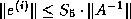 .
.
Next:
When or is
Up:
Stopping Criteria
Previous:
Stopping Criteria
Jack Dongarra
Mon Nov 20 08:52:54 EST 1995
When <IMG ALIGN=BOTTOM SRC="http://www.netlib.org/utk/papers/templates/_22900_tex2html_wrap6695.gif">
or <IMG ALIGN=BOTTOM SRC="http://www.netlib.org/utk/papers/templates/_22900_tex2html_wrap6959.gif">
is not readily available
Next:
Estimating
Up:
Stopping Criteria
Previous:
More Details about
It is possible to design an iterative algorithm for which
or
is not directly available,
although this is not the case for any algorithms in this book.
For completeness, however, we discuss stopping criteria in this case.
For example, if ones ``splits''
to get the iterative
method  , then the
natural residual to compute is
, then the
natural residual to compute is
 .
In other words, the residual
.
In other words, the residual  is the same as the residual of the
preconditioned system
is the same as the residual of the
preconditioned system 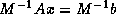 . In this case, it is
hard to interpret
as a backward error for the original system
, so we may instead derive a forward error bound
. In this case, it is
hard to interpret
as a backward error for the original system
, so we may instead derive a forward error bound
 .
Using this as a stopping criterion requires an estimate of
.
Using this as a stopping criterion requires an estimate of
 .
In the case of methods based on
splitting
, we have
.
In the case of methods based on
splitting
, we have  ,
and
,
and  .
.
Another example is an implementation of the preconditioned conjugate
gradient algorithm which computes  instead of
(the
implementation in this book computes the latter). Such an
implementation could use the stopping criterion
instead of
(the
implementation in this book computes the latter). Such an
implementation could use the stopping criterion  as in Criterion 5. We
may also use it to get the forward error bound
as in Criterion 5. We
may also use it to get the forward error bound  , which could also
be used in a stopping criterion.
, which could also
be used in a stopping criterion.
Jack Dongarra
Mon Nov 20 08:52:54 EST 1995
Estimating <IMG ALIGN=BOTTOM SRC="http://www.netlib.org/utk/papers/templates/_22900_tex2html_wrap6665.gif">
Next:
Stopping when progress
Up:
Stopping Criteria
Previous:
When or is
Bounds on the error
inevitably rely on bounds for
,
since  . There is a large number of problem dependent
ways to estimate
; we mention a few here.
. There is a large number of problem dependent
ways to estimate
; we mention a few here.
When a splitting
is used to get an iteration

then the matrix whose
inverse norm we need is  . Often, we know how to estimate
 if the splitting is a standard one such as Jacobi or SOR,
and the matrix
has special characteristics such as Property A.
Then we may estimate
if the splitting is a standard one such as Jacobi or SOR,
and the matrix
has special characteristics such as Property A.
Then we may estimate  .
.
When
is symmetric positive definite, and Chebyshev acceleration with
adaptation of parameters is being used, then at each step the algorithm
estimates the largest and smallest eigenvalues  and
and
 of
anyway.
Since
is symmetric positive definite,
of
anyway.
Since
is symmetric positive definite,
 .
.
This adaptive estimation is often done using the Lanczos algorithm
(see section
),
which can usually provide good estimates of the
largest (rightmost) and smallest (leftmost) eigenvalues of a symmetric matrix
at the cost of a few matrix-vector multiplies.
For general nonsymmetric
, we may apply
the Lanczos method to
or
,
and use the fact that
 .
.
It is also possible to estimate  provided one is willing
to solve a few systems of linear equations with
and
as coefficient
matrices. This is often done with dense linear system solvers, because the
extra cost of these systems is
provided one is willing
to solve a few systems of linear equations with
and
as coefficient
matrices. This is often done with dense linear system solvers, because the
extra cost of these systems is  , which is small compared to the cost
 of the LU decomposition (see Hager
[121],
Higham
[124] and Anderson, et al.
[3]).
This is not the case for iterative solvers, where the cost of these
solves may well be several times as much as the original linear system.
Still, if many linear systems with the same coefficient matrix and
differing right-hand-sides are to be solved, it is a viable method.
of the LU decomposition (see Hager
[121],
Higham
[124] and Anderson, et al.
[3]).
This is not the case for iterative solvers, where the cost of these
solves may well be several times as much as the original linear system.
Still, if many linear systems with the same coefficient matrix and
differing right-hand-sides are to be solved, it is a viable method.
The approach in the last paragraph also lets us estimate the alternate
error bound  .
This may be much smaller than the simpler
.
This may be much smaller than the simpler
 in the
case where the rows of
are badly scaled; consider the case of a
diagonal matrix
with widely varying diagonal entries. To
compute
in the
case where the rows of
are badly scaled; consider the case of a
diagonal matrix
with widely varying diagonal entries. To
compute  , let
, let  denote the diagonal
matrix with diagonal entries equal to the entries of
; then
denote the diagonal
matrix with diagonal entries equal to the entries of
; then
 (see Arioli, Demmel and Duff
[5]).
(see Arioli, Demmel and Duff
[5]).  can be estimated using the
technique in the last paragraph since multiplying by
can be estimated using the
technique in the last paragraph since multiplying by
 or
or  is no harder than multiplying
by
and
is no harder than multiplying
by
and  and also by
, a diagonal matrix.
and also by
, a diagonal matrix.
Next:
Stopping when progress
Up:
Stopping Criteria
Previous:
When or is
Jack Dongarra
Mon Nov 20 08:52:54 EST 1995
Stopping when progress is no longer being made
Next:
Accounting for floating
Up:
Stopping Criteria
Previous:
Estimating
In addition to limiting the total amount of work by limiting the
maximum number of iterations one is willing to do, it is also natural
to consider stopping when no apparent progress is being made.
Some methods, such as Jacobi and SOR, often exhibit nearly monotone
linear convergence, at least after some initial transients, so it
is easy to recognize when convergence degrades. Other methods, like
the conjugate gradient method, exhibit ``plateaus'' in their convergence,
with the residual norm stagnating at a constant value for many iterations
before decreasing again; in principle there can be many such plateaus
(see Greenbaum and Strakos
[110]) depending on the problem.
Still other methods, such as CGS, can appear
wildly nonconvergent for a large number of steps before the residual begins
to decrease; convergence may continue to be erratic from step to step.
In other words, while it is a good idea to have a criterion that stops
when progress towards a solution is no longer being made, the
form of such a criterion is both method and problem dependent.
Jack Dongarra
Mon Nov 20 08:52:54 EST 1995
Accounting for floating point errors
Next:
Data Structures
Up:
Stopping Criteria
Previous:
Stopping when progress
The error bounds discussed in this section are subject to floating
point errors, most of which are innocuous, but which deserve some discussion.
The infinity norm  requires the fewest
floating point operations to compute, and cannot overflow or cause other
exceptions if the
requires the fewest
floating point operations to compute, and cannot overflow or cause other
exceptions if the  are themselves finite
. On the other hand, computing
are themselves finite
. On the other hand, computing
 in the most straightforward manner
can easily overflow or lose accuracy to underflow even when the true result
is far from either the overflow or underflow thresholds. For this reason,
a careful implementation for computing
without this danger
is available (subroutine snrm2 in the BLAS
[72]
[144]),
but it is more expensive than computing
in the most straightforward manner
can easily overflow or lose accuracy to underflow even when the true result
is far from either the overflow or underflow thresholds. For this reason,
a careful implementation for computing
without this danger
is available (subroutine snrm2 in the BLAS
[72]
[144]),
but it is more expensive than computing  .
.
Now consider computing the residual
by forming the
matrix-vector product  and then subtracting
, all in floating
point arithmetic with relative precision
. A standard error
analysis shows that the error
and then subtracting
, all in floating
point arithmetic with relative precision
. A standard error
analysis shows that the error  in the computed
is bounded by
in the computed
is bounded by
 , where
 is typically bounded by
  , and
usually closer to
, and
usually closer to  . This is why one should not choose
 in Criterion 1, and why Criterion 2 may not
be satisfied by any method.
This uncertainty in the value of
induces an uncertainty in the error
of
at most
in Criterion 1, and why Criterion 2 may not
be satisfied by any method.
This uncertainty in the value of
induces an uncertainty in the error
of
at most
 .
A more refined bound is that the error
.
A more refined bound is that the error  in the
th component of
is bounded by
times the
th component of
in the
th component of
is bounded by
times the
th component of
 , or more tersely
.
This means the uncertainty in
is really bounded by
, or more tersely
.
This means the uncertainty in
is really bounded by
 .
This last quantity can be estimated inexpensively provided solving systems
with
and
as coefficient matrices is inexpensive (see the last
paragraph of §
).
Both these bounds can be severe overestimates of the uncertainty in
,
but examples exist where they are attainable.
.
This last quantity can be estimated inexpensively provided solving systems
with
and
as coefficient matrices is inexpensive (see the last
paragraph of §
).
Both these bounds can be severe overestimates of the uncertainty in
,
but examples exist where they are attainable.
Next:
Data Structures
Up:
Stopping Criteria
Previous:
Stopping when progress
Jack Dongarra
Mon Nov 20 08:52:54 EST 1995
Data Structures
Next:
Survey of Sparse
Up:
Related Issues
Previous:
Accounting for floating
The efficiency of any of the iterative methods considered in previous
sections is determined primarily by the performance of the
matrix-vector product and the preconditioner solve, and therefore on
the storage scheme used for the matrix and the preconditioner. Since
iterative methods are typically used on sparse matrices, we will
review here a number of sparse storage formats.
Often, the storage scheme used
arises naturally from the specific application problem.
Storage scheme: The way elements of a matrix are stored
in the memory of a computer. For dense matrices, this can be
the decision to store rows or columns consecutively.
For sparse matrices, common storage schemes avoid storing zero elements;
as a result they involve integer data describing where the stored elements
fit into the global matrix.
In this section we will review some of the more popular sparse matrix
formats that are used in numerical software packages such as ITPACK
[140] and NSPCG
[165].
After surveying the various formats, we demonstrate how the
matrix-vector product and an incomplete factorization solve are
formulated using two of the sparse matrix formats.
Jack Dongarra
Mon Nov 20 08:52:54 EST 1995
Iterative Methods
Next:
Overview of the
Up:
Templates for the Solution
Previous:
What Methods Are
The term ``iterative method'' refers to a wide range of techniques
that use successive approximations to obtain more accurate solutions
to a linear system at each step. In this book we will cover two types
of iterative methods.
Stationary methods are older, simpler to understand
and implement, but usually not as effective.
Nonstationary methods are a relatively recent
development; their analysis is usually harder to understand, but they
can be highly effective. The nonstationary methods we present are
based on the idea of sequences of orthogonal vectors. (An exception
is the Chebyshev
iteration method, which is based on
orthogonal polynomials.)
Stationary iterative method: Iterative method that performs
in each iteration the same operations on the current iteration vectors.
Nonstationary iterative method: Iterative method that
has iteration-dependent coefficients.
Dense matrix: Matrix for which the number of zero elements
is too small to warrant specialized algorithms.
Sparse matrix: Matrix for which the number of zero elements
is large enough that algorithms avoiding operations on zero elements
pay off. Matrices derived from partial differential equations typically
have a number of nonzero elements that is proportional to the matrix size,
while the total number of matrix elements is the square of the matrix size.
The rate at which an iterative method converges depends greatly on the
spectrum of the coefficient matrix. Hence, iterative methods usually
involve a second matrix that transforms the coefficient matrix into
one with a more favorable spectrum. The transformation matrix is
called a preconditioner.
A good preconditioner improves the convergence of the iterative method,
sufficiently to overcome the extra cost of constructing and applying
the preconditioner. Indeed, without a preconditioner the iterative
method may even fail to converge.
Jack Dongarra
Mon Nov 20 08:52:54 EST 1995
Survey of Sparse Matrix Storage Formats
Next:
Compressed Row Storage
Up:
Data Structures
Previous:
Data Structures
If the coefficient matrix
is sparse, large-scale linear systems
of the form
can be most
efficiently solved if the
zero elements of
are not stored. Sparse storage schemes allocate
contiguous storage in memory for
the nonzero elements of the matrix, and perhaps a limited number of
zeros. This, of course, requires a scheme for knowing
where the elements fit into the full matrix.
There are many methods for
storing the data (see for instance Saad
[186]
and Eijkhout
[87]).
Here we will discuss Compressed Row and Column Storage, Block Compressed
Row Storage, Diagonal Storage, Jagged Diagonal Storage, and Skyline
Storage.
Jack Dongarra
Mon Nov 20 08:52:54 EST 1995
Compressed Row Storage (CRS)
Next:
Compressed Column Storage
Up:
Survey of Sparse
Previous:
Survey of Sparse
The Compressed Row and Column (in the next section) Storage formats
are the most general: they make absolutely no assumptions about the
sparsity structure of the matrix, and they don't store any unnecessary
elements. On the other hand, they are not very efficient, needing an
indirect addressing step for every single scalar operation in a matrix-vector
product or preconditioner solve.
The Compressed Row Storage (CRS) format puts the subsequent nonzeros of the
matrix rows in contiguous memory locations.
Assuming we have a nonsymmetric sparse matrix
, we create
vectors:
one for floating-point numbers (val), and the other two for
integers (col_ind, row_ptr). The val vector
stores the values of the nonzero elements of the
matrix
, as they are traversed in a row-wise fashion.
The col_ind vector stores
the column indexes of the elements in the val vector.
That is, if  then
then  .
The row_ptr vector stores
the locations in the val vector that start a row, that is,
if
then
.
The row_ptr vector stores
the locations in the val vector that start a row, that is,
if
then  .
By convention, we define
.
By convention, we define  , where
  is
the number of nonzeros in the matrix
. The storage savings for this
approach is significant. Instead of storing
is
the number of nonzeros in the matrix
. The storage savings for this
approach is significant. Instead of storing  elements,
we need only
elements,
we need only  storage locations.
As an example, consider the nonsymmetric matrix
defined by
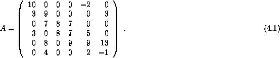
The CRS format for this matrix is then specified by the arrays
{val, col_ind, row_ptr} given below


.
If the matrix
is symmetric, we need only store the upper (or
lower) triangular portion of the matrix. The trade-off is
a more complicated algorithm with a somewhat different pattern of data access.
Jack Dongarra
Mon Nov 20 08:52:54 EST 1995
Compressed Column Storage (CCS)
Next:
Block Compressed Row
Up:
Survey of Sparse
Previous:
Compressed Row Storage
Analogous to Compressed Row Storage there is Compressed Column
Storage (CCS), which is also called the Harwell-Boeing
sparse matrix format
[78]. The CCS format is identical to the
CRS format except that the columns of
are stored (traversed) instead
of the rows. In other words, the CCS format is the CRS format
for
.
The CCS format is specified by the
arrays
{val, row_ind, col_ptr}, where
row_ind stores the row indices of each nonzero, and col_ptr
stores the index of the elements in val which start a column of
.
The CCS format for the matrix
in (
) is
given by


.
Jack Dongarra
Mon Nov 20 08:52:54 EST 1995
Block Compressed Row Storage (BCRS)
Next:
Compressed Diagonal Storage
Up:
Survey of Sparse
Previous:
Compressed Column Storage
If the sparse matrix
is comprised of square
dense blocks of nonzeros in some regular pattern, we can modify
the CRS (or CCS) format to exploit such block patterns. Block
matrices typically arise from the discretization of partial differential
equations in which there are several degrees of freedom associated
with a grid point. We then partition the matrix in small blocks with
a size equal to the number of degrees of freedom, and treat each
block as a dense matrix, even though it may have some zeros.
If
is the dimension of each block and  is the number of nonzero
blocks in the
matrix
, then the total storage
needed is
is the number of nonzero
blocks in the
matrix
, then the total storage
needed is  .
The block
dimension
.
The block
dimension  of
is then defined by
of
is then defined by  .
.
Similar to the CRS format, we require
arrays for the BCRS format:
a rectangular array for floating-point numbers (
val( ,
, ,
)) which stores the nonzero blocks in
(block) row-wise fashion, an integer array (col_ind(
))
which stores the actual column indices in the original matrix
of
the (
,
)) which stores the nonzero blocks in
(block) row-wise fashion, an integer array (col_ind(
))
which stores the actual column indices in the original matrix
of
the ( ) elements of the nonzero blocks, and a pointer
array (row_blk(
) elements of the nonzero blocks, and a pointer
array (row_blk( )) whose entries point to the beginning of
each block row in val(:,:,:) and col_ind(:). The
savings in storage locations and reduction in indirect addressing for
BCRS over CRS can be significant for matrices with a large
.
)) whose entries point to the beginning of
each block row in val(:,:,:) and col_ind(:). The
savings in storage locations and reduction in indirect addressing for
BCRS over CRS can be significant for matrices with a large
.
Jack Dongarra
Mon Nov 20 08:52:54 EST 1995
Compressed Diagonal Storage (CDS)
Next:
Jagged Diagonal Storage
Up:
Survey of Sparse
Previous:
Block Compressed Row
If the matrix
is banded with bandwidth that is fairly constant
from row to row,
then it is worthwhile to take advantage of this
structure in the storage scheme by storing subdiagonals of the matrix
in consecutive locations. Not only can we eliminate the vector
identifying the column and row, we can pack the nonzero elements in such a
way as to make the matrix-vector product more efficient.
This storage scheme is particularly useful if the matrix arises from
a finite element or finite difference discretization on a tensor
product grid.
We say that the matrix  is
banded if there are nonnegative constants
,
, called the left and
right halfbandwidth, such
that
only if
is
banded if there are nonnegative constants
,
, called the left and
right halfbandwidth, such
that
only if  . In this case, we can
allocate for the matrix
an array val(1:n,-p:q).
The declaration with reversed dimensions (-p:q,n) corresponds to the
LINPACK band format
[73], which unlike CDS,
does not allow for an
efficiently vectorizable matrix-vector multiplication if
. In this case, we can
allocate for the matrix
an array val(1:n,-p:q).
The declaration with reversed dimensions (-p:q,n) corresponds to the
LINPACK band format
[73], which unlike CDS,
does not allow for an
efficiently vectorizable matrix-vector multiplication if  is small.
Usually, band formats involve storing some zeros. The CDS
format may even contain some array elements that do not
correspond to matrix elements at all.
Consider the nonsymmetric matrix
defined by
Using the CDS format, we
store this matrix
in an array of dimension (6,-1:1) using
the mapping

Hence, the rows of the val(:,:) array are
.
Notice the two zeros corresponding to non-existing matrix elements.
A generalization of the CDS format more suitable for manipulating
general sparse matrices on vector supercomputers is discussed by
Melhem in
[154]. This variant of CDS uses a stripe data structure to store the matrix
. This structure is
more efficient in storage in the case of varying bandwidth, but it
makes the matrix-vector product slightly more expensive, as it
involves a gather operation.
As defined in
[154],
a stripe in the
matrix
is a set of positions
 , where
  and
and  is a strictly increasing function.
Specifically, if
is a strictly increasing function.
Specifically, if  and
and  are in
,
then
are in
,
then

When computing the
matrix-vector product  using stripes, each
 element of
in stripe
element of
in stripe  is multiplied
with both
and
is multiplied
with both
and  and these products are
accumulated in
and these products are
accumulated in  and
and  , respectively. For
the nonsymmetric matrix
defined by
, respectively. For
the nonsymmetric matrix
defined by
the
stripes of the matrix
stored
in the rows of the val(:,:) array would be
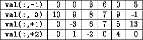
.
Next:
Jagged Diagonal Storage
Up:
Survey of Sparse
Previous:
Block Compressed Row
Jack Dongarra
Mon Nov 20 08:52:54 EST 1995
Jagged Diagonal Storage (JDS)
Next:
Skyline Storage (SKS)
Up:
Survey of Sparse
Previous:
Compressed Diagonal Storage
The Jagged Diagonal Storage format can be useful for the
implementation of iterative methods on parallel and vector processors
(see Saad
[185]). Like the Compressed Diagonal
format, it gives a vector length essentially of the size of the
matrix. It is more space-efficient than CDS at the cost of a
gather/scatter operation.
A simplified form of JDS, called ITPACK storage or Purdue
storage, can be described as follows. In the matrix
from (
) all elements are shifted left:
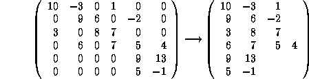
after which the columns are stored consecutively. All rows are padded
with zeros on the right to give them equal length. Corresponding to
the array of matrix elements val(:,:),
an array of column indices, col_ind(:,:) is also stored:
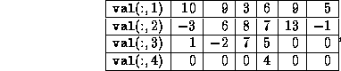
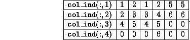
It is clear that the padding zeros in this structure may be a
disadvantage, especially if the bandwidth of the matrix varies strongly.
Therefore, in the CRS format, we
reorder the rows of the matrix decreasingly according to
the number of nonzeros per row. The compressed and permuted diagonals
are then stored in a linear array. The new data structure is called
jagged diagonals.
The number of jagged diagonals is equal to
the number of nonzeros in the first row, i.e., the largest
number of nonzeros in any row of
. The data structure to
represent the
matrix
therefore consists of a permutation
array (perm(1:n)) which reorders the rows, a floating-point array
(jdiag(:)) containing the jagged diagonals in succession,
an integer array (col_ind(:)) containing the corresponding column
indices, and finally a pointer array (jd_ptr(:)) whose elements
point to the beginning of each jagged diagonal. The advantages
of JDS for matrix multiplications are discussed by Saad in
[185].
The JDS format for the above matrix
in using the linear arrays
{perm, jdiag, col_ind, jd_ptr}
is given below (jagged diagonals are separated by semicolons)


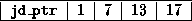
.
Next:
Skyline Storage (SKS)
Up:
Survey of Sparse
Previous:
Compressed Diagonal Storage
Jack Dongarra
Mon Nov 20 08:52:54 EST 1995
Skyline Storage (SKS)
Next:
Matrix vector products
Up:
Survey of Sparse
Previous:
Jagged Diagonal Storage
The final storage scheme we consider is for skyline matrices, which
are also called variable band or profile matrices (see Duff, Erisman
and Reid
[80]). It is mostly of importance in direct solution
methods, but it can be used for handling the diagonal blocks in block
matrix factorization methods. A major advantage of solving linear
systems having skyline coefficient matrices is that when pivoting is
not necessary, the skyline structure is preserved during Gaussian
elimination. If the matrix is symmetric, we only store its lower
triangular part. A straightforward approach in storing the elements
of a skyline matrix is to place all the rows (in order) into a
floating-point array (val(:)), and then keep an integer array
(row_ptr(:)) whose elements point to the beginning of each row.
The column indices of the nonzeros stored in val(:) are easily
derived and are not stored.
For a nonsymmetric skyline matrix such as the one illustrated in
Figure
, we store the lower
triangular elements in SKS format, and store the upper triangular
elements in a column-oriented SKS format (transpose stored in row-wise
SKS format). These two separated substructures can be linked in
a variety of ways. One approach, discussed by Saad
in
[186], is to store each row of the lower triangular
part and each column of the upper triangular part contiguously into
the floating-point array (val(:)). An additional pointer is
then needed to determine where the diagonal elements, which separate
the lower triangular elements from the upper triangular elements, are
located.
Figure: Profile of a nonsymmetric skyline or variable-band
matrix.
Jack Dongarra
Mon Nov 20 08:52:54 EST 1995
Matrix vector products
Next:
CRS Matrix-Vector Product
Up:
Data Structures
Previous:
Skyline Storage (SKS)
In many of the iterative methods discussed earlier, both the product
of a matrix and that of its transpose times a vector are needed, that
is, given an input vector
we want to compute products

We will present
these algorithms for two of the storage formats
from §
: CRS and CDS.
Jack Dongarra
Mon Nov 20 08:52:54 EST 1995
CRS Matrix-Vector Product
Next:
CDS Matrix-Vector Product
Up:
Matrix vector products
Previous:
Matrix vector products
The matrix vector product
using CRS format can be
expressed in the usual way:
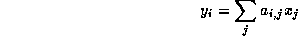
since this traverses the rows of the matrix
.
For an
matrix A, the
matrix-vector multiplication is given by
for i = 1, n
y(i) = 0
for j = row_ptr(i), row_ptr(i+1) - 1
y(i) = y(i) + val(j) * x(col_ind(j))
end;
end;
Since this method only multiplies nonzero matrix entries, the
operation count is
times the number of nonzero elements in
,
which is a significant savings over the dense operation requirement
of  .
.
For the transpose product  we cannot use the equation
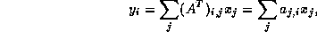
since this implies
traversing columns of the matrix, an extremely inefficient operation
for matrices stored in CRS format. Hence, we switch indices to

The matrix-vector multiplication involving
is then given by
for i = 1, n
y(i) = 0
end;
for j = 1, n
for i = row_ptr(j), row_ptr(j+1)-1
y(col_ind(i)) = y(col_ind(i)) + val(i) * x(j)
end;
end;
Both matrix-vector products above have largely the same structure, and
both use indirect addressing. Hence, their vectorizability properties
are the same on any given computer. However, the first product
(
) has a more favorable memory access pattern in that (per
iteration of the outer loop) it reads two vectors of data (a row of
matrix
and the input vector
) and writes one scalar. The
transpose product (
) on the other hand reads one element of
the input vector, one row of matrix
, and both reads and writes the
result vector
. Unless the machine on which these methods are
implemented has three separate memory paths (e.g., Cray Y-MP), the
memory traffic will then limit the performance. This is an
important consideration for RISC-based architectures.
Jack Dongarra
Mon Nov 20 08:52:54 EST 1995
CDS Matrix-Vector Product
Next:
Sparse Incomplete Factorizations
Up:
Matrix vector products
Previous:
CRS Matrix-Vector Product
If the
matrix
is
stored in CDS format, it is still possible to
perform a matrix-vector product
by either rows or columns, but this
does not take advantage of the CDS format. The idea
is to make a change in coordinates in the doubly-nested loop. Replacing
 we get

With the index
in the inner loop we see that the
expression  accesses the
th diagonal of the matrix
(where the main diagonal has number 0).
accesses the
th diagonal of the matrix
(where the main diagonal has number 0).
The algorithm will now have a doubly-nested loop with the outer loop
enumerating the diagonals diag=-p,q with
and
the
(nonnegative) numbers of diagonals to the left and right of the main
diagonal. The bounds for the inner loop follow from the requirement
that

The algorithm becomes
for i = 1, n
y(i) = 0
end;
for diag = -diag_left, diag_right
for loc = max(1,1-diag), min(n,n-diag)
y(loc) = y(loc) + val(loc,diag) * x(loc+diag)
end;
end;
The transpose matrix-vector product
is a minor variation of the
algorithm above. Using the update formula

we obtain
for i = 1, n
y(i) = 0
end;
for diag = -diag_right, diag_left
for loc = max(1,1-diag), min(n,n-diag)
y(loc) = y(loc) + val(loc+diag, -diag) * x(loc+diag)
end;
end;
The memory access for the CDS-based matrix-vector product
(or
) is
three vectors per inner iteration. On the other hand, there is no
indirect addressing, and the algorithm is vectorizable with vector
lengths of essentially the matrix order
. Because of the regular data
access, most machines can perform this algorithm
efficiently by keeping three base registers and using simple offset
addressing.
Jack Dongarra
Mon Nov 20 08:52:54 EST 1995
Templates for the Solution of Linear Systems: <BR>Building Blocks for Iterative Methods<A NAME=tex2html1 HREF="http://www.netlib.org/utk/papers/templates/footnode.html#22">
<IMG ALIGN=BOTTOM ALT="gif" SRC="http://www.netlib.org/utk/icons/foot_motif.gif">
</A>

Next:
How to Use
=25pt
-8pt
Eijk-hout
Templates for the Solution of Linear Systems:
Building Blocks for Iterative Methods
Richard Barrett
,Michael Berry
,
Tony F. Chan
,
James Demmel
,
June M. Donato
,
Jack Dongarra  ,
,
Victor Eijkhout ,
Roldan Pozo
Charles Romine ,
and
Henk Van der Vorst
This book is also available in Postscript from over the Internet.
To retrieve the postscript file you can use one of the following methods:
-
anonymous ftp to www.netlib.org
cd templates
get templates.ps
quit
-
from any machine on the Internet type:
rcp anon@www.netlib.org:templates/templates.ps templates.ps
-
send email to netlib@ornl.gov and in the message type:
send templates.ps from templates
The url for this book is
http://www.netlib.org/templates/Templates.html .
A bibtex reference for this book follows:
@BOOK{templates,
AUTHOR = {R. Barrett and M. Berry and T. F. Chan and J. Demmel and
J. Donato and J. Dongarra and V. Eijkhout and R. Pozo and
C. Romine, and H. Van der Vorst },
TITLE = {Templates for the Solution of Linear Systems:
Building Blocks for Iterative Methods},
PUBLISHER = {SIAM},
YEAR = {1994},
ADDRESS = {Philadelphia, PA} }
Jack Dongarra
Mon Nov 20 08:52:54 EST 1995
Contents


Next:
Foreword
Up:
Parallel Computing Works
Previous:
Parallel Computing Works
Guy Robinson
Wed Mar 1 10:19:35 EST 1995
Foreword

Next:
1 Introduction
Up:
Parallel Computing Works
Previous:
Contents
This book describes a set of application and systems software
research projects undertaken by the Caltech Concurrent
Computation Program (C P) from 1983-1990. This parallel
computing activity is organized so that applications with similar
algorithmic and software challenges are grouped together. Thus,
one can not only learn that parallel computing is effective on a
broad range of problems but also why it works, what algorithms
are needed, and what features the software should support. The
description of the software has been updated through 1993 to
reflect the current interests of Geoffrey Fox, now at Syracuse
University but still working with many C
P) from 1983-1990. This parallel
computing activity is organized so that applications with similar
algorithmic and software challenges are grouped together. Thus,
one can not only learn that parallel computing is effective on a
broad range of problems but also why it works, what algorithms
are needed, and what features the software should support. The
description of the software has been updated through 1993 to
reflect the current interests of Geoffrey Fox, now at Syracuse
University but still working with many C P collaborators
through the auspices of the NSF Center for Research in Parallel
Computation (CRPC).
P collaborators
through the auspices of the NSF Center for Research in Parallel
Computation (CRPC).
Many C P members wrote sections of this book. John
Apostolakis wrote Section 7.4; Clive Baillie, Sections 4.3, 4.4, 7.2
and 12.6; Vas Bala, Section 13.2; Ted Barnes, Section 7.3; Roberto
Battitti, Sections 6.5, 6.7, 6.8 and 9.9; Rob Clayton, Section 18.2;
Dave Curkendall, Section 18.3; Hong Ding, Sections 6.3 and 6.4;
David Edelsohn, Section 12.8; Jon Flower, Sections 5.2, 5.3, 5.4
and 13.5; Tom Gottschalk, Sections 9.8 and 18.4; Gary Gutt,
Section 4.5; Wojtek Furmanski, Chapter 17; Mark Johnson,
Section 14.2; Jeff Koller, Sections 13.4 and 15.2; Aron
Kuppermann, Section 8.2; Paulette Liewer, Section 9.3; Vince
McKoy, Section 8.3; Paul Messina, Chapter 2; Steve Otto, Sections
6.6, 11.4, 12.7, 13.6 and 14.3; Jean Patterson, Section 9.4; Francois
Pepin, Section 12.5; Peter Reiher, Section 15.3; John Salmon,
Section 12.4; Tony Skjellum, Sections 9.5, 9.6 and Chapter 16;
Michael Speight, Section 7.6; Eric Van de Velde, Section 9.7;
David Walker, Sections 6.2 and 8.1; Brad Werner, Section 9.2;
Roy Williams, Sections 11.1, 12.2, 12.3 and Chapter 10. Geoffrey
Fox wrote the remaining text. Appendix B describes many of the key
C
P members wrote sections of this book. John
Apostolakis wrote Section 7.4; Clive Baillie, Sections 4.3, 4.4, 7.2
and 12.6; Vas Bala, Section 13.2; Ted Barnes, Section 7.3; Roberto
Battitti, Sections 6.5, 6.7, 6.8 and 9.9; Rob Clayton, Section 18.2;
Dave Curkendall, Section 18.3; Hong Ding, Sections 6.3 and 6.4;
David Edelsohn, Section 12.8; Jon Flower, Sections 5.2, 5.3, 5.4
and 13.5; Tom Gottschalk, Sections 9.8 and 18.4; Gary Gutt,
Section 4.5; Wojtek Furmanski, Chapter 17; Mark Johnson,
Section 14.2; Jeff Koller, Sections 13.4 and 15.2; Aron
Kuppermann, Section 8.2; Paulette Liewer, Section 9.3; Vince
McKoy, Section 8.3; Paul Messina, Chapter 2; Steve Otto, Sections
6.6, 11.4, 12.7, 13.6 and 14.3; Jean Patterson, Section 9.4; Francois
Pepin, Section 12.5; Peter Reiher, Section 15.3; John Salmon,
Section 12.4; Tony Skjellum, Sections 9.5, 9.6 and Chapter 16;
Michael Speight, Section 7.6; Eric Van de Velde, Section 9.7;
David Walker, Sections 6.2 and 8.1; Brad Werner, Section 9.2;
Roy Williams, Sections 11.1, 12.2, 12.3 and Chapter 10. Geoffrey
Fox wrote the remaining text. Appendix B describes many of the key
C P contributors, with brief biographies.
C P's research depended on the support of many sponsors;
central support for major projects was given by the Department
of Energy and the Electronic Systems Division of the USAF.
Other federal sponsors were the Joint Tactical Fusion office,
NASA, NSF and the National Security Agency. C
P's research depended on the support of many sponsors;
central support for major projects was given by the Department
of Energy and the Electronic Systems Division of the USAF.
Other federal sponsors were the Joint Tactical Fusion office,
NASA, NSF and the National Security Agency. C P's start up
was only possible due to two private donations from the Parsons
and System Development Foundations. Generous corporate
support came from ALCOA, Digital Equipment, General
Dynamics, General Motors, Hitachi, Hughes, IBM, INTEL,
Lockheed, McDonnell Douglas, MOTOROLA, Nippon Steel,
nCUBE, Sandia National Laboratories, and Shell.
P's start up
was only possible due to two private donations from the Parsons
and System Development Foundations. Generous corporate
support came from ALCOA, Digital Equipment, General
Dynamics, General Motors, Hitachi, Hughes, IBM, INTEL,
Lockheed, McDonnell Douglas, MOTOROLA, Nippon Steel,
nCUBE, Sandia National Laboratories, and Shell.
Production of this book would have been impossible without
the dedicated help of Richard Alonso, Lisa Deyo, Keri Arnold, Blaise
Canzian and especially Terri Canzian.
Next:
1 Introduction
Up:
Parallel Computing Works
Previous:
Contents
Guy Robinson
Wed Mar 1 10:19:35 EST 1995
1 Introduction
Next:
1.1 Introduction
Up:
Parallel Computing Works
Previous:
Foreword
Guy Robinson
Wed Mar 1 10:19:35 EST 1995
1.1 Introduction
Next:
1.2 The National Vision
Up:
1 Introduction
Previous:
1 Introduction
This book describes the activities of the Caltech Concurrent Computation
Program (C P). This was a seven-year project (1983-1990), focussed
on the question, ``Can parallel computers be used effectively for large
scale scientific computation?'' The title of the book, ``Parallel
Computing Works,'' reveals our belief that we answered the question in
the affirmative, by implementing numerous scientific applications on
real parallel computers and doing computations that produced new
scientific results. In the process of doing so, C
P). This was a seven-year project (1983-1990), focussed
on the question, ``Can parallel computers be used effectively for large
scale scientific computation?'' The title of the book, ``Parallel
Computing Works,'' reveals our belief that we answered the question in
the affirmative, by implementing numerous scientific applications on
real parallel computers and doing computations that produced new
scientific results. In the process of doing so, C P helped design
and build several new computers, designed and implemented basic system
software, developed algorithms for frequently used mathematical
computations on massively parallel machines, devised performance models
and measured the performance of many computers, and created a
high-performance computing facility based exclusively on parallel computers.
While the initial focus of C
P helped design
and build several new computers, designed and implemented basic system
software, developed algorithms for frequently used mathematical
computations on massively parallel machines, devised performance models
and measured the performance of many computers, and created a
high-performance computing facility based exclusively on parallel computers.
While the initial focus of C P was the hypercube architecture
developed by C. Seitz at Caltech, many of the methods developed and
lessons learned have been applied successfully on other massively
parallel architectures.
P was the hypercube architecture
developed by C. Seitz at Caltech, many of the methods developed and
lessons learned have been applied successfully on other massively
parallel architectures.
Of course, C P was only one of many projects contributing to this
field and so the contents of this book are only representative of the
important activities in parallel computing during the last ten years.
However, we believe that the project did address a wide range of issues
and applications areas. Thus, a book focussed on C
P was only one of many projects contributing to this
field and so the contents of this book are only representative of the
important activities in parallel computing during the last ten years.
However, we believe that the project did address a wide range of issues
and applications areas. Thus, a book focussed on C P has some general
interest. We do, of course, cite other activities but surely not
completely. Other general references which the reader will find
valuable are [
Almasi:89a
], [
Andrews:91a
], [
Arbib:90a
],
[
Blelloch:90a
], [
Brawer:89a
], [
Doyle:91a
], [
Duncan:90a
],
[
Fox:88a
], [
Golub:89a
], [
Hayes:89a
], [
Hennessy:91a
],
[
Hillis:85a
], [
Hockney:81a
], [
Hord:90a
], [
Hwang:89a
],
[
IEEE:91a
], [
Laksh:90a
], [
Lazou:87a
], [Messina:87a;91d],
[
Schneck:87a
], [
Skerrett:92a
], [
Stone:91a
], [
Trew:91a
],
[
Zima:91a
].
P has some general
interest. We do, of course, cite other activities but surely not
completely. Other general references which the reader will find
valuable are [
Almasi:89a
], [
Andrews:91a
], [
Arbib:90a
],
[
Blelloch:90a
], [
Brawer:89a
], [
Doyle:91a
], [
Duncan:90a
],
[
Fox:88a
], [
Golub:89a
], [
Hayes:89a
], [
Hennessy:91a
],
[
Hillis:85a
], [
Hockney:81a
], [
Hord:90a
], [
Hwang:89a
],
[
IEEE:91a
], [
Laksh:90a
], [
Lazou:87a
], [Messina:87a;91d],
[
Schneck:87a
], [
Skerrett:92a
], [
Stone:91a
], [
Trew:91a
],
[
Zima:91a
].
C P was both a technical and social experiment. It involved a wide
range of disciplines working together to understand the hardware,
software, and algorithmic (applications) issues in parallel computing.
Such multidisciplinary
activities are
generally considered of growing relevance to many new academic and
research activities-including the federal high-performance computing
and communication initiative. Many of the participants of C
P was both a technical and social experiment. It involved a wide
range of disciplines working together to understand the hardware,
software, and algorithmic (applications) issues in parallel computing.
Such multidisciplinary
activities are
generally considered of growing relevance to many new academic and
research activities-including the federal high-performance computing
and communication initiative. Many of the participants of C P are
no longer at Caltech, and this has positive and negative messages.
C
P are
no longer at Caltech, and this has positive and negative messages.
C P was not set up in a traditional academic fashion since its core
interdisciplinary field, computational science, is not well understood
or implemented either nationally or in specific universities. This is
explored further in Chapter
20
. C
P was not set up in a traditional academic fashion since its core
interdisciplinary field, computational science, is not well understood
or implemented either nationally or in specific universities. This is
explored further in Chapter
20
. C P has led to flourishing
follow-on projects at Caltech, Syracuse University, and elsewhere.
These differ from C
P has led to flourishing
follow-on projects at Caltech, Syracuse University, and elsewhere.
These differ from C P just as parallel computing has changed from an
exploratory field to one that is in a transitional stage into
development, production, and exploitation.
P just as parallel computing has changed from an
exploratory field to one that is in a transitional stage into
development, production, and exploitation.
Next:
1.2 The National Vision
Up:
1 Introduction
Previous:
1 Introduction
Guy Robinson
Wed Mar 1 10:19:35 EST 1995
1.2 The National Vision
for ParallelComputation
Next:
1.3 Caltech Concurrent Computation
Up:
1 Introduction
Previous:
1.1 Introduction
The technological driving force behind parallel computing is
VLSI,
or very large scale integration-the same technology
that created the personal computer and workstation market over the last
decade. In 1980, the Intel 8086 used 50,000 transistors; in 1992,
the latest Digital alpha RISC chip contains 1,680,000 transistors-a
factor of 30 increase. The dramatic improvement in chip density comes
together with an increase in clock speed and improved design so that
the alpha performs better by a factor of over one thousand on
scientific problems than the 8086-8087 chip pair of the early 1980s.
The increasing density of transistors on a chip follows directly from a
decreasing feature size which is now  for the alpha. Feature
size will continue to decrease and by the year 2000, chips with
50 million transistors are expected to be available. What can we do
with all these transistors?
for the alpha. Feature
size will continue to decrease and by the year 2000, chips with
50 million transistors are expected to be available. What can we do
with all these transistors?
With around a million transistors on a chip, designers were able to move
full mainframe functionality to about  of a chip. This
enabled the personal computing and workstation revolutions. The next
factors of ten increase in transistor density must go into some form of
parallelism by replicating several CPUs on a single chip.
of a chip. This
enabled the personal computing and workstation revolutions. The next
factors of ten increase in transistor density must go into some form of
parallelism by replicating several CPUs on a single chip.
By the year 2000, parallelism is thus inevitable to all computers, from
your children's video game to personal computers, workstations, and
supercomputers. Today we see it in the larger machines as we replicate many
chips and printed circuit boards to build systems as arrays of
nodes, each unit of which is some variant of the microprocessor. This
is illustrated in Figure 1.1 (Color Plate), which shows an
nCUBE
parallel supercomputer with 64 identical nodes on
each board-each node is a single-chip CPU with additional memory
chips. To be useful, these nodes must be linked in some way and this
is still a matter of much research and experimentation. Further, we
can argue as to the most appropriate node to replicate; is it a
``small'' node as in the nCUBE of Figure 1.1 (Color Plate), or more
powerful ``fat'' nodes such as those offered in CM-5 and Intel
Touchstone shown in Figures 1.2 and 1.3 (Color Plates) where each node
is a sophisticated multichip printed circuit board? However, these
details should not obscure the basic point: Parallelism allows one to
build the world's fastest and most cost-effective supercomputers.
Figure 1.1 :
The nCUBE-2 node and its integration into
a board. Upto 128 of these boards can be combined into a single
supercomputer.
Figure 1.2 :
The CM-5 produced by Thinking Machines.
Figure 1.3 :
The DELTA Touchstone parallel
supercomputer produced by Intel and installed at Caltech.
Parallelism may only be critical today for supercomputer vendors and
users. By the year 2000, all computers will have to address the
hardware, algorithmic, and software issues implied by parallelism. The
reward will be amazing performance and the opening up of new fields;
the price will be a major rethinking and reimplementation of software,
algorithms, and applications.
This vision and its consequent issues are now well understood and
generally agreed. They provided the motivation in 1981 when
C P's first roots were formed. In those days, the vision was blurred
and controversial. Many believed that parallel computing would not
work.
P's first roots were formed. In those days, the vision was blurred
and controversial. Many believed that parallel computing would not
work.
President Bush instituted, in 1992, the five-year federal High
Performance Computing and Communications (HPCC) Program. This will spur the
development of the technology described above and is focussed on the
solution of grand challenges shown in Figure 1.4 (Color Plate). These
are fundamental problems in science and engineering, with broad economic
and scientific impact, whose solution could be advanced by applying
high-performance computing techniques and resources.
Figure 1.4:
Grand Challenge Appications. Some major
applications which will be enabled by parallel supercomputers. The computer
performance numbers are given in more detail in color figure 2.1.
The activities of several federal agencies have been coordinated in
this program. The Advanced Research Projects Agency (ARPA) is developing
the basic technologies which is applied to the grand challenges by
the Department of Energy (DOE), the National Aeronautics and Space Agency
(NASA), the National Science Foundation (NSF), the National Institute of Health
(NIH), the Environmental Protection Agency (EPA), and the National
Oceanographic and Atmospheric Agency (NOAA). Selected activities
include the mapping of the human genome in DOE, climate modelling in
DOE and NOAA, coupled structural and airflow simulations of advanced
powered lift and a high-speed civil transport by NASA.
More generally, it is clear that parallel computing can only realize its
full potential and be commercially successful if it is accepted in the
real world of industry and government applications. The clear U.S.
leadership over Europe and Japan in high-performance computing offers
the rest of the U.S. industry the opportunity of gaining global
competitive advantage.
Some of these industrial opportunities are discussed in
Chapter
19
. Here we note some interesting possibilities which
include
-
use in the oil industry for both seismic
analysis of new
oil fields and the reservoir simulation of existing fields;
-
environmental modelling of past and potential pollution in air
and ground;
-
fluid flow simulations of aircraft, and general vehicles, engines,
air-conditioners, and other turbomachinery; integration of structural
analysis with the computational fluid dynamics
of airflow; car crash simulation;
-
integrated design and manufacturing systems;
-
design of new drugs for the pharmaceutical industry by modelling
new compounds;
-
simulation of electromagnetic
and network
properties of electronic systems-from new components to full printed
circuit boards;
-
identification of new materials with interesting
properties such as superconductivity;
-
simulation of electrical and gas distribution systems to optimize
production and response to failures;
-
production of animated films and educational and entertainment
uses such as simulation of virtual worlds in theme parks and other
virtual reality applications;
-
support of geographic information systems including real-time
analysis of data from satellite sensors in NASA's ``Mission to Planet
Earth.''
-
A relatively unexplored area is known as ``command and control''
in the military area and ``decision support'' or ``information
processing'' in the civilian applications. These combine large
databases
with extensive computation. In the
military, the database could be sensor information and the processing a
multitrack Kalman filter.
Commercially, the database
could be the nation's medicaid records and the processing would aim at cost
containment by identifying anomalies and inconsistencies.
-
servers in multimedia networks set up by cable and telecommunication
companies. These servers will provide video, information, and
simulation on demand to home, education, and industrial users.
C P did not address such large-scale problems. Rather, we
concentrated on major academic applications. This fit the
experience of the Caltech faculty who led most of the C
P did not address such large-scale problems. Rather, we
concentrated on major academic applications. This fit the
experience of the Caltech faculty who led most of the C P teams, and
further academic applications are smaller and cleaner than large-scale
industrial problems. One important large-scale C
P teams, and
further academic applications are smaller and cleaner than large-scale
industrial problems. One important large-scale C P application was
a military simulation described in Chapter
18
and produced
by Caltech's Jet Propulsion Laboratory. C
P application was
a military simulation described in Chapter
18
and produced
by Caltech's Jet Propulsion Laboratory. C P chose the correct and
only computations on which to cut its parallel computing teeth. In
spite of the focus on different applications, there are many
similarities between the vision and structure of C
P chose the correct and
only computations on which to cut its parallel computing teeth. In
spite of the focus on different applications, there are many
similarities between the vision and structure of C P and today's
national effort. It may even be that today's grand challenge teams can
learn from C
P and today's
national effort. It may even be that today's grand challenge teams can
learn from C P's experience.
Next:
1.3 Caltech Concurrent Computation
Up:
1 Introduction
Previous:
1.1 Introduction
Guy Robinson
Wed Mar 1 10:19:35 EST 1995
1.3 Caltech Concurrent Computation Program
Next:
1.4 How Parallel Computing
Up:
1 Introduction
Previous:
1.2 The National Vision
C P's origins dated to an early collaboration between the physics and
computer science departments at Caltech in bringing up UNIX on the physics
department's VAX 11/780. As an aside, we note this was motivated by the
development of the Symbolic Manipulation Program (SMP) by Wolfram and
collaborators; this project has now grown into the well-known system
Mathematica. Carver Mead from computer science urged physics to get
back to them if we had insoluble large scale computational needs. This
comment was reinforced in May, 1981 when Mead gave a physics
colloquium on VLSI, Very Large Scale Integration, and the opportunities
it opened up. Fox, in the audience, realized that quantum
chromodynamics (QCD, Section
4.3
), now using up all free cycles on
the VAX 11/780, was naturally parallelizable and could take advantage of
the parallel machines promised by VLSI. Thus, a seemingly modest
interdisciplinary interaction-a computer scientist lecturing to
physicists-gave birth to a large interdisciplinary project, C
P's origins dated to an early collaboration between the physics and
computer science departments at Caltech in bringing up UNIX on the physics
department's VAX 11/780. As an aside, we note this was motivated by the
development of the Symbolic Manipulation Program (SMP) by Wolfram and
collaborators; this project has now grown into the well-known system
Mathematica. Carver Mead from computer science urged physics to get
back to them if we had insoluble large scale computational needs. This
comment was reinforced in May, 1981 when Mead gave a physics
colloquium on VLSI, Very Large Scale Integration, and the opportunities
it opened up. Fox, in the audience, realized that quantum
chromodynamics (QCD, Section
4.3
), now using up all free cycles on
the VAX 11/780, was naturally parallelizable and could take advantage of
the parallel machines promised by VLSI. Thus, a seemingly modest
interdisciplinary interaction-a computer scientist lecturing to
physicists-gave birth to a large interdisciplinary project, C P.
Further, our interest in QCD stemmed from the installation of the
VAX 11/780 to replace our previous batch computing using a remote
CDC7600
. This more attractive computing environment, UNIX
on a VAX 11/780, encouraged theoretical physics graduate students to
explore computation.
P.
Further, our interest in QCD stemmed from the installation of the
VAX 11/780 to replace our previous batch computing using a remote
CDC7600
. This more attractive computing environment, UNIX
on a VAX 11/780, encouraged theoretical physics graduate students to
explore computation.
During the summer of 1981, Fox's research group, especially
Eugene Brooks and Steve Otto, showed that effective concurrent
algorithms could be developed, and we presented our conclusion to the
Caltech computer scientists. This presentation led to the plans,
described in a national context in Chapter
2
, to produce the first
hypercube, with Chuck Seitz and his student Erik DeBenedictis
developing the hardware and Fox's group the QCD applications and
systems software. The physics group did not understand what a
hypercube was at that stage, but agreed with the computer scientists
because the planned six-dimensional hypercube was isomorphic to a
 three-dimensional mesh,
a topology
whose relevance a physicist could appreciate. With the generous help
of the computer scientists, we gradually came to understand the
hypercube topology with its general advantage (maximum distance between
nodes is
three-dimensional mesh,
a topology
whose relevance a physicist could appreciate. With the generous help
of the computer scientists, we gradually came to understand the
hypercube topology with its general advantage (maximum distance between
nodes is  ) and its specific feature of including a rich
variety of mesh topologies. Here
N
is the total number of nodes in
the concurrent computer. We should emphasize that this understanding
of the relevance of concurrency to QCD was not particularly novel; it
followed from ideas already known from earlier concurrent machines such
as the Illiac IV. We were, however, fortunate to investigate the
issues at a time when microprocessor technology (in particular the
Intel 8086/8087) allowed one to build large (in terms of number of
nodes) cost-effective concurrent computers with interesting performance
levels. The QCD problem was also important in helping ensure that the
initial Cosmic Cube
was built with sensible design
choices; we were fortunate that in choosing parameters, such as
memory size, appropriate for QCD, we also realized a machine of general
capability.
) and its specific feature of including a rich
variety of mesh topologies. Here
N
is the total number of nodes in
the concurrent computer. We should emphasize that this understanding
of the relevance of concurrency to QCD was not particularly novel; it
followed from ideas already known from earlier concurrent machines such
as the Illiac IV. We were, however, fortunate to investigate the
issues at a time when microprocessor technology (in particular the
Intel 8086/8087) allowed one to build large (in terms of number of
nodes) cost-effective concurrent computers with interesting performance
levels. The QCD problem was also important in helping ensure that the
initial Cosmic Cube
was built with sensible design
choices; we were fortunate that in choosing parameters, such as
memory size, appropriate for QCD, we also realized a machine of general
capability.
While the 64-node Cosmic Cube was under construction, Fox wandered
around Caltech and the associated Jet Propulsion Laboratory explaining
parallel computing and, in particular, the Cosmic Cube to scientists in
various disciplines who were using ``large'' (by the standards of 1981)
scale computers. To his surprise, all the problems being tackled on
conventional machines by these scientists seemed to be implementable on
the Cosmic Cube. This was the origin of C P, which identified the
Caltech-JPL applications team, whose initial participants are noted in
Table
4.2
. Fox, Seitz, and these scientists prepared the
initial proposals which established and funded C
P, which identified the
Caltech-JPL applications team, whose initial participants are noted in
Table
4.2
. Fox, Seitz, and these scientists prepared the
initial proposals which established and funded C P in the summer of
1983. Major support was obtained from the Department of Energy and the
Parsons and System Development Foundation. Intel made key initial
contributions of chips to the Cosmic Cube and follow-on machines. The
Department of Energy remained the central funding support for C
P in the summer of
1983. Major support was obtained from the Department of Energy and the
Parsons and System Development Foundation. Intel made key initial
contributions of chips to the Cosmic Cube and follow-on machines. The
Department of Energy remained the central funding support for C P
throughout its seven years, 1983 to 1990.
P
throughout its seven years, 1983 to 1990.
The initial C P proposals were focussed on the question:
``Is the hypercube an effective computer for large-scale scientific
computing?''
Our approach was simple: Build or acquire interesting
hardware and provide the intellectual and physical infrastructure to
allow leading application scientists and engineers to both develop
parallel algorithms and codes, and use them to address important
problems. Often we liked to say that C P
P
``used real hardware and real software to solve real problems.''
Our project showed initial success, with the approximately ten
applications of Table
4.2
developed in the first year. We both
showed good performance on the hypercube and developed a performance
model which is elaborated in Chapter
3
. A major
activity at this time was the design and development of the necessary
support software, termed CrOS and later developed into the
commercial software Express described in Chapter
5
.
Not only was the initial hardware applicable to a wide range of
problems, but our software model proved surprisingly useful. CrOS was
originally designed by Brooks as the ``mailbox communication system''
and we initially targeted the regular synchronous problems typified in
Chapter
4
. Only later did we realize that it supported quite
efficiently the irregular and non-local communication needs of more
general problems. This generalization is represented as an evolutionary
track of Express in Chapter
5
and for a new
communication system Zipcode in Section
16.1
developed from
scratch for general asynchronous irregular problems.
Although successful, we found many challenges and intriguing questions
opened up by C P's initial investigation into parallel computing.
Further, around 1985, the DOE and later the NSF made substantial
conventional supercomputer
(Cray, Cyber, ETA) time available to
applications scientists. Our Cosmic Cube
and the
follow-on Mark II machines were very competitive with the VAX 11/780,
but not with the performance offered by the CRAY X-MP. Thus, internal
curiosity and external pressures moved C
P's initial investigation into parallel computing.
Further, around 1985, the DOE and later the NSF made substantial
conventional supercomputer
(Cray, Cyber, ETA) time available to
applications scientists. Our Cosmic Cube
and the
follow-on Mark II machines were very competitive with the VAX 11/780,
but not with the performance offered by the CRAY X-MP. Thus, internal
curiosity and external pressures moved C P in the direction of
computer science: still developing real software but addressing new
parallel algorithms and load-balancing techniques rather than a
production application. This phase of C
P in the direction of
computer science: still developing real software but addressing new
parallel algorithms and load-balancing techniques rather than a
production application. This phase of C P is summarized in
[
Angus:90a
], [Fox:88a;88b].
P is summarized in
[
Angus:90a
], [Fox:88a;88b].
Around 1988, we returned to our original goal with a focus on parallel
supercomputers. We no longer concentrated on the hypercube, but rather
asked such questions as [
Fox:88v
],
``What are the cost, technology, and software trade-offs that will drive
the design of future parallel supercomputers?''
and as a crucial (and harder) question:
``What is the appropriate software environment for parallel machines and
how should one develop it?''
We evolved from the initial 8086/8087, 80286/80287 machines to the
internal JPL Mark IIIfp and commercial nCUBE-1
and CM-2
described in Chapter
2
. These were still ``rough, difficult
to use machines'' but had performance capabilities competitive with
conventional supercomputers.
This book largely describes work in the last three years of C P when
we developed a series of large scale applications on these parallel
supercomputers. Further, as described in Chapters
15
,
16
, and
17
, we developed prototypes and ideas for
higher level software environments which could accelerate and ease the
production of parallel software. This period also saw an explosion of
interest in the use of parallel computing outside Caltech. Much of
this research used commercial hypercubes which partly motivated our
initial discoveries and successes on the in-house machines at Caltech.
This rapid technology transfer was in one sense gratifying, but it also
put pressure on C
P when
we developed a series of large scale applications on these parallel
supercomputers. Further, as described in Chapters
15
,
16
, and
17
, we developed prototypes and ideas for
higher level software environments which could accelerate and ease the
production of parallel software. This period also saw an explosion of
interest in the use of parallel computing outside Caltech. Much of
this research used commercial hypercubes which partly motivated our
initial discoveries and successes on the in-house machines at Caltech.
This rapid technology transfer was in one sense gratifying, but it also
put pressure on C P which was better placed to blaze new trails than
to perform the more programmatic research which was now appropriate.
P which was better placed to blaze new trails than
to perform the more programmatic research which was now appropriate.
An important and unexpected discovery in C P was in the education and
the academic support for interdisciplinary research. Many of the
researchers, especially graduate students in C
P was in the education and
the academic support for interdisciplinary research. Many of the
researchers, especially graduate students in C P, evolved to be
``computational scientists.'' Not traditional physicists, chemists, or
computer scientists but rather something in between. We believe that
this interdisciplinary education and expertise was critical for C
P, evolved to be
``computational scientists.'' Not traditional physicists, chemists, or
computer scientists but rather something in between. We believe that
this interdisciplinary education and expertise was critical for C P's
success and, as discussed in Chapter
20
, it should be encouraged in
more universities [Fox:91f;92d].
P's
success and, as discussed in Chapter
20
, it should be encouraged in
more universities [Fox:91f;92d].
Further information about C P can be found in our annual reports and two
reviews.
P can be found in our annual reports and two
reviews.
[Fox:84j;84k;85c;85e;85i;86f;87c;87d;88v;88oo;89i;89n;89cc;89dd;90o]
Next:
1.4 How Parallel Computing
Up:
1 Introduction
Previous:
1.2 The National Vision
Guy Robinson
Wed Mar 1 10:19:35 EST 1995
1.4 How Parallel Computing Works
Next:
2 Technical Backdrop
Up:
1 Introduction
Previous:
1.3 Caltech Concurrent Computation
C P's research showed that
-
PCW:
-
Parallel Computers work in a large class of scientific
and engineering computations.
The book quantifies and exemplifies this assertion.
In Chapter
2
, we provide the national overview of parallel
computing activities during the last decade. Chapter
3
is somewhat speculative as it attempts to provide a framework to quantify
the previous
PCW
statement.
We will show that, more precisely, parallel computing only works in a
``scaling'' fashion in a special class of problems which we call
synchronous and loosely synchronous.
By scaling, we mean that the parallel implementation will efficiently
extend to systems with large numbers of nodes without levelling off of
the speedup obtained. These concepts are quantified in
Chapter
3
with a simple performance model described in
detail in [
Fox:88a
].
The book is organized with applications and software issues growing in
complexity in later chapters. Chapter
4
describes the cleanest
regular synchronous applications which included many of our initial
successes. However, we already see the essential points:
-
DD:
-
Domain decomposition (or data parallelism) is a
universal source of scalable parallelism
-
MP:
-
 software model was a simple explicit
message passing with each node of a parallel processor running conventional
sequential code communicating via subroutine call with other nodes.
software model was a simple explicit
message passing with each node of a parallel processor running conventional
sequential code communicating via subroutine call with other nodes.
CrOS and its follow-on Express, described in Chapter
5
,
support this software paradigm. Explicit message passing is still an
important software model and in many cases, the only viable approach to
high-performance parallel implementations on MIMD machines.
Chapters
6
through
9
confirm these lessons
with an extension to more irregular problems. Loosely synchronous
problem classes are harder to parallelize, but still use the basic
principles
DD
and
MP
. Chapter
7
describes a special
class,
embarrassingly parallel
, of applications where scaling
parallelism is guaranteed by the independence of separate components of
the problem.
Chapters
10
and
11
describe parallel computing tools
developed within C P. DIME supports parallel mesh generation and
adaptation, and its use in general finite element codes. Initially, we
thought load balancing would be a major stumbling block for parallel computing
because formally it is an NP-complete
(intractable)
optimization
problem. However, effective
heuristic
methods were developed which avoid the
exponential time complexity of NP-complete
problems
by searching for good but not exact minima.
P. DIME supports parallel mesh generation and
adaptation, and its use in general finite element codes. Initially, we
thought load balancing would be a major stumbling block for parallel computing
because formally it is an NP-complete
(intractable)
optimization
problem. However, effective
heuristic
methods were developed which avoid the
exponential time complexity of NP-complete
problems
by searching for good but not exact minima.
In Chapter
12
, we describe the most complex irregular loosely
synchronous problems which include some of the hardest problems tackled
in C P.
P.
As described earlier, we implemented essentially all the applications
described in the book using explicit user-generated message passing.
In Chapter
13
, we describe our initial efforts to produce
a higher level data-parallel Fortran environment, which should be able to
provide a more attractive software environment for the user. High
Performance Fortran has been adopted as an informal industry standard
for this language.
In Chapter
14
, we describe the very difficult asynchronous
problem class for which scaling parallel algorithms and the correct
software model are less clear. Chapters
15
,
16
, and
17
describe four software models, Zipcode, MOOSE, Time Warp, and
MOVIE which tackle asynchronous and the mixture of asynchronous and
loosely synchronous problems one finds in the complex system
simulations and analysis typical of many real-world
problems. Applications of this class are described in
Chapter
18
, with the application of
Section
18.3
being an event-driven simulation-an
important class of difficult-to-parallelize asynchronous applications.
In Chapter
19
we look to the future and describe some
possibilities for the use of parallel computers in industry. Here we
note that C P, and much of the national enterprise, concentrated on
scientific and engineering computations. The examples and ``proof''
that parallel computing works are focussed in this book on such
problems. However, this will
not
be the dominant industrial
use of parallel computers where information processing is most
important. This will be used for decision support in the military and
large corporations, and to supply video, information and simulation
``on demand'' for homes, schools, and other institutions. Such
applications have recently been termed
national challenges
to
distinguish them from the large scale
grand challenges
, which
underpinned the initial HPCC initiative [
FCCSET:94a
]. The lessons
C
P, and much of the national enterprise, concentrated on
scientific and engineering computations. The examples and ``proof''
that parallel computing works are focussed in this book on such
problems. However, this will
not
be the dominant industrial
use of parallel computers where information processing is most
important. This will be used for decision support in the military and
large corporations, and to supply video, information and simulation
``on demand'' for homes, schools, and other institutions. Such
applications have recently been termed
national challenges
to
distinguish them from the large scale
grand challenges
, which
underpinned the initial HPCC initiative [
FCCSET:94a
]. The lessons
C P and others have learnt from scientific computations will have
general applicability across the wide range of industrial problems.
P and others have learnt from scientific computations will have
general applicability across the wide range of industrial problems.
Chapter
20
includes a discussion of education in computational
science-an unexpected byproduct of C P-and other retrospective
remarks. The appendices list the C
P-and other retrospective
remarks. The appendices list the C P reports including those not
cited directly in this book. Some information is available
electronically by mailing citlib@caltech.edu.
P reports including those not
cited directly in this book. Some information is available
electronically by mailing citlib@caltech.edu.
Next:
2 Technical Backdrop
Up:
1 Introduction
Previous:
1.3 Caltech Concurrent Computation
Guy Robinson
Wed Mar 1 10:19:35 EST 1995
2 Technical Backdrop
Next:
2.1 Introduction
Up:
Parallel Computing Works
Previous:
1.4 How Parallel Computing
Guy Robinson
Wed Mar 1 10:19:35 EST 1995
2.1 Introduction
Next:
2.2 Hardware Trends
Up:
2 Technical Backdrop
Previous:
2 Technical Backdrop
This chapter surveys activities related to parallel computing that took place
around the time that C P was an active project, primarily during the
1980s. The major areas that are covered are hardware, software, research
projects, and production uses of parallel computers. In each case, there is
no attempt to present a comprehensive list or survey of all the work that was
done in that area. Rather, the attempt is to identify some of the major
events during the period.
P was an active project, primarily during the
1980s. The major areas that are covered are hardware, software, research
projects, and production uses of parallel computers. In each case, there is
no attempt to present a comprehensive list or survey of all the work that was
done in that area. Rather, the attempt is to identify some of the major
events during the period.
There are two major motivations for creating and using parallel computer
architectures. The first is that, as surveyed in Section
1.2
parallelism is the only avenue to achieve vastly higher speeds than are
possible now from a single processor. This was the primary motivation for
initiating C P. Table
2.1
demonstrates dramatically the
rather slow increase in speed of single-processor systems for one particular
brand of supercomputer, CRAYs,
the most popular
supercomputer in the world. Figure 2.1 (Color Plate) shows a more
comprehensive sample of computer performance, measured in operations
per second, from the 1940s extrapolated through the year 2000.
P. Table
2.1
demonstrates dramatically the
rather slow increase in speed of single-processor systems for one particular
brand of supercomputer, CRAYs,
the most popular
supercomputer in the world. Figure 2.1 (Color Plate) shows a more
comprehensive sample of computer performance, measured in operations
per second, from the 1940s extrapolated through the year 2000.
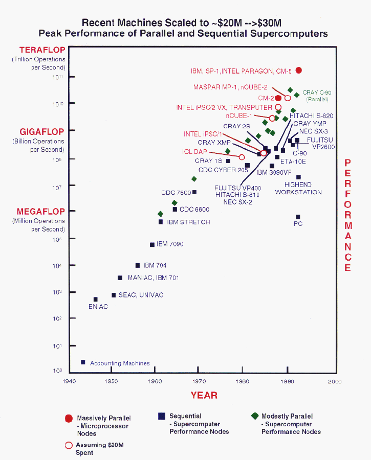
Figure 2.1:
Historical trends of peak computer
performance. In some cases, we have scaled up parallel performance to
correspond to a configuration that would cost approximately $20 million.
A second motivation for the use of parallel architectures is that they should
be considerably cheaper than sequential machines for systems of moderate
speeds; that is, not necessarily supercomputers but instead minicomputers or
mini-supercomputers would be cheaper to produce for a given performance level
than the equivalent sequential system.
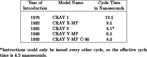
Table 2.1:
Cycle Times
At the beginning of the 1980s, the goals of research in parallel computer
architectures were to achieve much higher speeds than could be obtained from
sequential architectures and to get much better price performance through
the use of parallelism than would be possible from sequential machines.
Guy Robinson
Wed Mar 1 10:19:35 EST 1995
2.2 Hardware Trends
Next:
2.2.1 Parallel Scientific Computers
Up:
2 Technical Backdrop
Previous:
2.1 Introduction
Guy Robinson
Wed Mar 1 10:19:35 EST 1995
2.2.1 Parallel Scientific Computers Before 1980
Next:
2.2.2 Early 1980s
Up:
2.2 Hardware Trends
Previous:
2.2 Hardware Trends
There were parallel computers before 1980, but they did not have a
widespread impact on scientific computing. The activities of the 1980s
had a much more dramatic effect. Still, a few systems stand out as
having made significant contributions that were taken advantage of in
the 1980s. The first is the Illiac IV
[
Hockney:81b
]. It did not seem like a significant advance to many
people at the time, perhaps because its performance was only moderate,
it was difficult to program, and had low reliability. The best
performance achieved was two to six times the speed of a
CDC 7600
. This was obtained on various computational fluid
dynamics codes. For many other programs, however, the performance was
lower than that of a CDC 7600,
which was the supercomputer of
choice during the early and mid-1970s. The Illiac was a research
project, not a commercial product, and it was reputed to be
so expensive that it was not realistic for others to replicate it.
While the Illiac IV did not inspire the masses to become interested in
parallel computing, hundreds of people were involved in its use and in
projects related to providing better software tools and better
programming languages for it. They first learned how to do parallel
computing on the Illiac IV and many of them went on to make
significant contributions to parallel computing in the 1980s.
The Illiac was an SIMD
computer-single-instruction,
multiple-data architecture. It had 32 processing elements, each of
which was a processor with its own local memory; the processors were
connected in a ring. High-level languages such as Glypnyr and Fortran
were available for the Illiac IV. Glypnyr was reminiscent of Fortran
and had extensions for parallel and array processing.
The ICL Distributed Array Processor (DAP)
[
DAP:79a
] was
a commercial product; a handful of machines were sold, mainly in
England where it was designed and built. Its characteristics were that
it had either 1K or 4K one-bit processors arranged in a square plane,
each connected in rectangular fashion to its nearest neighbors. Like
the Illiac IV, it was an SIMD
system. It required an ICL
mainframe as a front end. The ICL DAP was used for many university
science applications. The University of Edinburgh, in particular, used
it for a number of real computations in physics, chemistry,
and other fields [Wallace:84a;87a].
The ICL DAP had a substantial impact on
scientific computing culture, primarily in Europe. ICL did try to
market it in the United States, but was never effective in doing so;
the requirement for an expensive ICL mainframe as a host was a
substantial negative factor.
A third important commercial parallel computer in the 1970s was the
Goodyear Massively Parallel Processor (MPP)
[
Batcher:85a
], [Karplus:87a, pp. 157-166].
Goodyear started building SIMD computers in 1969, but all except the
MPP were sold to the military and to the Federal Aviation
Administration for air traffic control. In the late 1970s, Goodyear
produced the MPP which was installed at Goddard Space Flight Center, a
NASA research center, and used for a variety of scientific
applications. The MPP attracted attention because it did achieve high
speeds on a few applications, speeds that, in the late 1970s and early
1980s, were remarkable-measured in the hundreds of MFLOPS in a few
cases. The MPP had 16K one-bit processors, each with local memory, and
was programmed in Pascal and Assembler.
In summary, the three significant scientific parallel computers of the
1970s were the Illiac IV, the ICL DAP, and the Goodyear MPP. All were
SIMD computers. The DAP and the MPP were fine-grain systems based on
single-bit processors, whereas the Illiac IV was a large-grain SIMD
system. The other truly significant high-performance (but not
parallel) computer of the 1970s was the CRAY 1, which was introduced in
1976. The CRAY 1 was a single-processor vector computer and as such it
can also be classified as a special kind of SIMD computer because it
had vector instructions. With a single vector instruction, one causes
up to 64 data pairs to be operated on.
There were significant and seminal activities in parallel
computing in the 1970s both from the standpoint of design and construction of
systems and in the actual scientific use of the systems. However, the level
of activity of parallel computing in the 1970s was modest compared to what
followed in the 1980s.
Next:
2.2.2 Early 1980s
Up:
2.2 Hardware Trends
Previous:
2.2 Hardware Trends
Guy Robinson
Wed Mar 1 10:19:35 EST 1995
2.2.2 Early 1980s
Next:
2.2.3 Birth of the
Up:
2.2 Hardware Trends
Previous:
2.2.1 Parallel Scientific Computers
In contrast to the 1970s, in the early 1980s it was MIMD
(multiple
instruction, multiple data) computers that dominated the activity in parallel
computing. The first of these was the Denelcor Heterogeneous Element
Processor (HEP).
The HEP attracted widespread attention
despite its terrible cost performance because of its many interesting
hardware features that facilitated programming. The Denelcor HEP was
acquired by several institutions, including Los Alamos, Argonne
National Laboratory, Ballistic Research Laboratory, and Messerschmidt
in Germany. Messerschmidt was the only installation that used it for
real applications. The others, however, used it extensively for
research on parallel algorithms. The HEP hardware supported both
fine-grain and large-grain parallelism. Any one processor had an
instruction pipeline that provided parallelism at the single
instruction level. Instructions from separate processes (associated
with separate user programs or tasks) were put into hardware queues and
scheduled for execution once the required operands had been fetched
from memory into registers, again under hardware control. Instructions
from up to 128 processes could share the instruction execution
pipeline. The latter had eight stages; all instructions except
floating-point divide took eight machine cycles to execute. Up to 16
processors could be linked to perform large-grain MIMD computations.
The HEP had an extremely efficient synchronization mechanism through a
full-empty bit associated with every word of memory. The bit was
automatically set to indicate whether the word had been rewritten since
it had last been written into and could be set to indicate that the
memory location had been read. The value of the full-empty bit could
be checked in one machine cycle. Fortran, C, and Assembler could be
used to program the HEP. It had a UNIX environment and was front-ended
by a minicomputer. Because Los Alamos and Argonne made their HEPs
available for research purposes to people who were interested in
learning how to program parallel machines or who were involved in
parallel algorithm research, hundreds of people became familiar with
parallel computing through the Denelcor HEP [
Laksh:85a
].
A second computer that was important in the early 1980s, primarily
because it exposed a large number of computational scientists to
parallelism, was the CRAY X-MP/22, which was introduced in 1982.
Certainly, it had limited parallelism, namely only two processors;
still, it was a parallel computer. Since it was at the very high end
of performance, it exposed the hardcore scientific users to
parallelism, although initially mostly in a negative way. There was
not enough payoff in speed or cost to compensate for the effort that
was required to parallelize a program so that it would use both
processors: the maximum speedup would, of course, only be two.
Typically, it was less than two and the charging algorithms of most
computer centers generated higher charges for a program when it used
both processors than when it used only one. In a way, though, the
CRAY X-MP multiprocessor legitimized parallel processing, although
restricted to very large grain, very small numbers of processors. A
few years later, the IBM 3090 series had the same effect; the 3090 can
have up to six vector and scalar processors in one system. Memory is
shared among all processors.
Another MIMD system that was influential during the early 1980s was the
New York University Ultracomputer
[
Gottlieb:86a
] and a related system, the IBM RP3
[
Brochard:92a
], [
Brochard:92b
], [
Darema:87a
],
[
Pfister:85a
]. These systems were serious attempts to design and
demonstrate a shared-memory architecture that was scalable to very
large numbers of processors. They featured an interconnection network
between processors and memories that would avoid hot spots and
congestion. The fetch-and-add instruction that was invented by
Jacob Schwartz [
Schwartz:80a
] would avoid some of the congestion
problems in omega networks. Unfortunately, these systems took a great
deal of time to construct and it was the late 1980s before the IBM RP3
existed in a usable fashion. At that time, it had 64 processors but
each was so slow that it attracted comparatively little attention. The
architecture is certainly still considered to be an interesting one,
but far fewer users were exposed to these systems than to other designs
that were constructed more quickly and put in places that allowed a
large number of users to have at least limited access to the systems
for experimentation. Thus, the importance of the Ultracomputer and RP3
projects lay mainly in the concepts.
Next:
2.2.3 Birth of the
Up:
2.2 Hardware Trends
Previous:
2.2.1 Parallel Scientific Computers
Guy Robinson
Wed Mar 1 10:19:35 EST 1995
2.2.3 Birth of the Hypercube
Next:
2.2.4 Mid-1980s
Up:
2.2 Hardware Trends
Previous:
2.2.2 Early 1980s
Perhaps the most significant and influential parallel computer system
of the early 1980s was the Caltech Cosmic Cube
[
Seitz:85a
], developed by Charles Seitz and Geoffrey Fox. Since
it was the inspiration for the C P project, we describe it and its
immediate successors in some detail
[Fox:87d;88oo], [
Seitz:85a
].
P project, we describe it and its
immediate successors in some detail
[Fox:87d;88oo], [
Seitz:85a
].
The hypercube work at Caltech originated in May 1981 when, as
described in Chapter
1
, Fox attended a seminar by Carver Mead
on VLSI
and its implications for concurrency. As described
in more detail in Sections
4.1
and
4.3
, Fox realized that
he could use parallel computers for the lattice gauge
computations that were central to his research at the time and
that his group was running on a VAX 11/780. During the summer of 1981,
he and his students worked out an algorithm that he thought would be
parallel and tried it out on his VAX (simulating parallelism). The
natural architecture for the problems he wanted to compute was
determined to be a  three-dimensional grid, which
happens to be 64 processors (Figure
4.3
).
three-dimensional grid, which
happens to be 64 processors (Figure
4.3
).
In the fall of 1981 Fox approached Chuck Seitz about building a
suitable computer. After an exchange of seminars, Seitz showed great
interest in doing so and had funds to build a hypercube. Given Fox's
problem, a six-dimensional hypercube (64 processors) was set as the
target. Memory size of 128K was chosen after some debate;
applications people (chiefly Fox) wanted at least that much. A
trade-off was made between the number of processors and memory size. A
smaller cube would been built if larger memory had been chosen.
From the outset a key goal was to produce an architecture with
interprocessor communications that would scale well to a very large number
of processors. The features that led to the choice of the hypercube
topology specifically were the moderate growth in the number of
channels required as the number of processors increases, and the good
match between processor and memory speeds because memory is local.
The Intel 8086 was chosen because it was the only microprocessor available
at the time with a floating-point co-processor, the 8087. First, a
prototype 4-node system was built with wirewrap boards. It was
designed, assembled, and tested during the winter of 1981-82. In the
spring of 1982, message-passing software was designed and implemented on
the 4-node. Eugene Brooks' proposal of simple send/receive routines
was chosen and came to be known as the Crystalline Operating System
(CrOS), although it was never really an operating system.
In autumn of 1982, simple lattice problems were implemented on the
4-node by Steve Otto and others. CrOS and the computational algorithm
worked satisfactorily. By January 1983, Otto had the lattice gauge
applications program running on the 4-node. Table
4.2
details the many projects and publications stemming from this pioneering
work.
With the successful experience on the 4-node, Seitz proceeded to have
printed circuit boards designed and built. The 64-node Cosmic Cube was
assembled over the summer of 1983 and began operation in October 1983.
It has been in use ever since, although currently it is lightly
used.
The key characteristics of the Cosmic Cube are that it has 64 nodes,
each with an 8086/8087,  of memory, and communication
channels with 2 Mbits/sec peak speed between nodes (about 0.8 Mbits/sec
sustained in one direction). It is five feet long, six cubic feet in volume,
and draws 700 watts.
of memory, and communication
channels with 2 Mbits/sec peak speed between nodes (about 0.8 Mbits/sec
sustained in one direction). It is five feet long, six cubic feet in volume,
and draws 700 watts.
The Cosmic Cube provided a dramatic demonstration that multicomputers
could be built quickly, cheaply, and reliably. In terms of
reliability, for example, there were two hard failures in the first
560,000 node hours of operation-that is, during the first year of
operation. Its performance was low by today's standards, but it was
still between five and ten times the performance of a DEC VAX 11/780,
which was the system of choice for academic computer departments and
research groups in that time period. The manufacturing cost of the
system was $80,000, which at that time was about half the cost of a
VAX with a modest configuration. Therefore, the price performance was
on the order of 10 to 20 times better than a VAX 780. This estimate
does not take into account design and software development costs; on
the other hand, it was a one-of-a-kind system, so manufacturing costs
were higher than for a commercial product. Furthermore, it was clearly
a scalable architecture, and that is perhaps the most important feature
of that particular project.
In the period from October, 1983 to April, 1984 a 2500-hour run of a QCD
problem (Table
4.1
) was completed, achieved 95% efficiency, and
produced new scientific
results. This demonstrated that hypercubes are well-suited for QCD (as
are other architectures).
As described in Section
1.3
, during the fall of 1982 Fox surveyed many
colleagues at Caltech to determine whether they needed large-scale
computation in their research and began to examine those applications for
suitability to run on parallel computers. Note that this was before the
64-node Cosmic Cube was finished, but after the 4-node gave evidence that
approach was sound. The Caltech Concurrent Computation Program (C P) was
formed in Autumn of 1982. A decision was made to develop big, fast hypercubes
rather than rely on Crays. By the summer of 1984, the ten applications
of Table
4.2
were running on the Cosmic Cube [
Fox:87d
].
P) was
formed in Autumn of 1982. A decision was made to develop big, fast hypercubes
rather than rely on Crays. By the summer of 1984, the ten applications
of Table
4.2
were running on the Cosmic Cube [
Fox:87d
].
Two key shortcomings that were soon noticed were that too much time was
spent in communications and that high-speed external I/O
was not
available. The first was thought to be addressable with custom
communication chips.
In the summer of 1983, Fox teamed with Caltech's Jet Propulsion
Laboratory (JPL) to build bigger and better hypercubes. The first was
the Mark II, still based on 8086/8087 (no co-processor faster than 8087
was yet available), but with  memory, faster communications, and
twice as many nodes. The first 32 nodes began operating in September,
1984. Four 32-node systems and one 128-node were built. The latter
was completed in June, 1985 [
Fox:88oo
].
memory, faster communications, and
twice as many nodes. The first 32 nodes began operating in September,
1984. Four 32-node systems and one 128-node were built. The latter
was completed in June, 1985 [
Fox:88oo
].
The Caltech project inspired several industrial companies to build commercial
hypercubes. These included Intel, nCUBE
[
Karplus:87a
], Ametek
[
Seitz:88b
], and Floating Point Systems Corporation. Only two years
after the 64-node Caltech Cosmic Cube
was
operational, there were commercial products on the market and installed
at user sites.
With the next Caltech-JPL system, the Mark III, there was a switch to the
Motorola family of microprocessors. On each node the Mark III had
one Motorola 68020/68881 for computation and another 68020 for
communications. The two processors shared the  of node
memory. The first 32-node Mark III was operational in April, 1986.
The concept of dedicating a processor to communications
has influenced commercial product design, including recently introduced
systems.
of node
memory. The first 32-node Mark III was operational in April, 1986.
The concept of dedicating a processor to communications
has influenced commercial product design, including recently introduced
systems.
In the spring of 1986, a decision was made to build a variant of the
Mark III, the Mark IIIfp (originally dubbed the Mark IIIe). It was
designed to compete head-on with ``real'' supercomputers. The Mark IIIfp
has a daughter board at each node with the Weitek XL floating-point
chip set running at  , which gives a peak speed of
 . By January 1987, an 8-node Mark IIIfp was
operational. A 128-node system was built and in the spring of 1989 achieved
. By January 1987, an 8-node Mark IIIfp was
operational. A 128-node system was built and in the spring of 1989 achieved
 on two applications.
In summary, the hypercube family of computers enjoyed rapid development
and was used for scientific applications from the beginning. In the
period from 1982 to 1987, three generations of the family were designed, built,
and put into use at Caltech. The third generation (the Mark III) even
included a switch of microprocessor families. Within the same five
years, four commercial vendors produced and delivered computers with
hypercube architectures. By 1987, approximately 50 major applications
had been completed on Caltech hypercubes. Such rapid development and
adaption has few if any parallels. The remaining chapters of this book
are largely devoted to lessons from these applications and their
followers.
Next:
2.2.4 Mid-1980s
Up:
2.2 Hardware Trends
Previous:
2.2.2 Early 1980s
Guy Robinson
Wed Mar 1 10:19:35 EST 1995
2.2.4 Mid-1980s
Next:
2.2.5 Late 1980s
Up:
2.2 Hardware Trends
Previous:
2.2.3 Birth of the
During this period, many new systems were launched by commercial
companies, and several were quite successful in terms of sales. The
two most successful were the Sequent and the Encore
[Karplus:87a, pp. 111-126] products. Both were
shared-memory, bus-connected multiprocessors of moderate parallelism.
The maximum number of processors on the Encore product was 20; on the
Sequent machine initially 16 and later 30. Both provided an extremely
stable UNIX environment and were excellent for time-sharing. As such,
they could be considered VAX killers since VAXes were the time-sharing
system of choice in research groups in those days. The Sequent and the
Encore provided perhaps a cost performance better by a factor of 10, as
well as considerably higher total performance than could be obtained on
a VAX at that time. These systems were particularly useful for smaller
jobs, for time-sharing, and for learning to do parallel computing.
Perhaps their most impressive aspect was the reliability of both
hardware and software. They operated without interruption for months
at a time, just as conventional mini-supercomputers did. Their UNIX
operating system software was familiar to many users and, as mentioned
before, very stable. Unlike most parallel computers whose system
software requires years to mature, these systems had very stable and
responsive system software from the beginning.
Another important system during this period was the Alliant
[Karplus:87a, pp. 35-44]. The initial model
featured up to eight vector processors, each of moderate performance.
But when used simultaneously, they provided performance equivalent to a
sizable fraction of a CRAY processor. A unique feature at the time was
a Fortran compiler
that was quite good at automatic
vectorization and also reasonably good at parallelization. These
compiler features, coupled with its shared memory,
made this system relatively easy to use and to achieve reasonably good
performance. The Alliant also supported the C language, although
initially there was no vectorization or parallelization available in
C. The operating system was UNIX-based. Because of its reasonably
high floating-point performance and ease of use, the Alliant was one of
the first parallel computers that was used for real applications. The
Alliant was purchased by groups who wanted to do medium-sized
computations and even computations they would normally do on CRAYs.
This system was also used as a building block of the Cedar
architecture project led by D. Kuck [
Kuck:86a
].
Advances in compiling technology made wide-instruction word machines an
interesting and, for a few years, commercially viable architecture.
The Multiflow and Cydrome systems both had compilers that effectively
exploited very fine-grain parallelism and scheduling of floating-point
pipelines within the processing units. Both these systems attempted to
get parallelism at the instruction level from Fortran programs-the
so-called dusty decks that might have convoluted logic and thus be very
difficult to vectorize or parallelize in a large-grain sense. The
price performance of these systems was their main attraction. On the
other hand, because these systems did not scale to very high levels of
performance, they were relegated to the super-minicomputer arena. An
important contribution they made was to show dramatically how far
compiler technology had come in certain areas.
As was mentioned earlier, hypercubes were produced by Intel,
nCUBE,
Ametek, and Floating Point Systems Corporation in
the mid-1980s. Of these, the most significant product was the
nCUBE
with its high degree of integration and a configuration of up
to 1024 nodes [
Palmer:86a
], [
nCUBE:87a
]. It was pivotal in
demonstrating that massively parallel MIMD medium-grain computers are
practical. The nCUBE featured a complete processor on a single chip,
including all channels for connecting to the other nodes so that one
chip plus six memory chips constituted an entire node. They were
packaged on boards with 64 nodes so that the system was extremely
compact, air-cooled, and reliable. Caltech had an early 512-node
system, which was used in many C P calculations, and soon afterwards
Sandia National Laboratories installed the 1024-node system. A great
deal of scientific work was done on those two machines and they are
still in use. The 1024-node Sandia machine got the world's attention
by demonstrating speedups of 1000 for several applications
[
Gustafson:88a
]. This was particularly significant because it was
done during a period of active debate as to whether MIMD systems could
provide speedups of more than a hundred. Amdahl's law
[
Amdahl:67a
] was cited as a reason why it would not be
possible to get speedups greater than perhaps a hundred, even if one
used 1000 processors.
P calculations, and soon afterwards
Sandia National Laboratories installed the 1024-node system. A great
deal of scientific work was done on those two machines and they are
still in use. The 1024-node Sandia machine got the world's attention
by demonstrating speedups of 1000 for several applications
[
Gustafson:88a
]. This was particularly significant because it was
done during a period of active debate as to whether MIMD systems could
provide speedups of more than a hundred. Amdahl's law
[
Amdahl:67a
] was cited as a reason why it would not be
possible to get speedups greater than perhaps a hundred, even if one
used 1000 processors.
Towards the end of the mid-1980s, transputer-based
systems
[
Barron:83a
], [
Hey:88a
], both large and small, began to
proliferate, especially in Europe but also in the United States. The
T800 transputer was like the nCUBE processor, a single-chip system with
built-in communications channels, and it had respectable floating point
performance-a peak speed of nearly  and frequently
achieved speeds of 1/2 to
and frequently
achieved speeds of 1/2 to  . They provided a convenient
building block for parallel systems and were quite cost-effective.
Their prevalent use at the time was in boards with four or eight
transputers that were attached to IBM PCs, VAXes, or other workstations.
. They provided a convenient
building block for parallel systems and were quite cost-effective.
Their prevalent use at the time was in boards with four or eight
transputers that were attached to IBM PCs, VAXes, or other workstations.
Next:
2.2.5 Late 1980s
Up:
2.2 Hardware Trends
Previous:
2.2.3 Birth of the
Guy Robinson
Wed Mar 1 10:19:35 EST 1995
2.2.5 Late 1980s
Next:
2.2.6 Parallel Systems-1992
Up:
2.2 Hardware Trends
Previous:
2.2.4 Mid-1980s
By the late 1980s, truly powerful parallel systems began to
appear. The Meiko
system at Edinburgh University, is an
example; by 1989, that computer had 400 T800s [
Wallace:88a
]. The
system was being used for a number of traditional scientific
computations in physics, chemistry,
engineering, and
other areas [
Wexler:89a
]. The system software for
transputer-based systems had evolved to resemble the message-passing
system software available on hypercubes. Although the transputer's
two-dimensional mesh connection is in principle less efficient than
hypercube connections, for systems of moderate size (only a few hundred
processors), the difference is not significant for most applications.
Further, any parallel architecture deficiencies were counterbalanced by
the transputer's excellent communication channel performance.
Three new SIMD
fine-grain systems were introduced in the
late 1980s: the CM-2, the MasPar,
and a new version of
the DAP. The
CM-2
is a version of the original Connection
Machine
[Hillis:85a;87a]
that has been enhanced with
Weitek floating-point units, one for each 32 single-bit processors, and
optional large memory. In its largest configuration, such as is
installed at Los Alamos National Laboratory, there are 64K single-bit
processors, 2048 64-bit floating-point processors, and  of memory. The CM-2 has been measured at
  running the
unlimited Linpack benchmark solving a linear system of order 26,624 and
even higher performance on some applications, e.g.,
seismic
data processing [
Myczkowski:91a
] and QCD
[
Brickner:91b
], [
Liu:91a
]. It has attracted widespread
attention both because of its extremely high performance and its
relative ease of use [
Boghosian:90a
], [Hillis:86a;87b].
For problems that are
naturally data parallel, the CM Fortran language and compiler provide a
relatively easy way to implement programs and get high performance.
running the
unlimited Linpack benchmark solving a linear system of order 26,624 and
even higher performance on some applications, e.g.,
seismic
data processing [
Myczkowski:91a
] and QCD
[
Brickner:91b
], [
Liu:91a
]. It has attracted widespread
attention both because of its extremely high performance and its
relative ease of use [
Boghosian:90a
], [Hillis:86a;87b].
For problems that are
naturally data parallel, the CM Fortran language and compiler provide a
relatively easy way to implement programs and get high performance.
The MasPar and the DAP are smaller systems that are aimed more at
excellent price performance than at supercomputer levels of
performance. The new DAP is front-ended by Sun workstations or VAXes.
This makes it much more affordable and compatible with modern computing
environments than when it required an ICL front end. DAPs have been
built in ruggedized versions that can be put into vehicles, flown in
airplanes, and used on ships, and have found many uses in signal
processing and military applications. They are also used for general
scientific work. The MasPar is the newest SIMD system. Its
architecture constitutes an evolutionary approach of fine-grain SIMD
combined with enhanced floating-point performance coming from the use
of 4-bit (Maspar MP-1) or 32-bit (Maspar MP-2) basic SIMD units.
Standard 64-bit floating-point algorithms implemented on a (SIMD)
machine built around an
l
bit CPU take time of order  machine instructions. The DAP and CM-1,2 used
l=1
and here the CM-2
and later DAP models achieve floating-point performance with special
extra hardware rather than by increasing
l
.
machine instructions. The DAP and CM-1,2 used
l=1
and here the CM-2
and later DAP models achieve floating-point performance with special
extra hardware rather than by increasing
l
.
Two hypercubes became available just as the decade ended: the second
generation nCUBE,
popularly known as the nCUBE-2, and the
Intel iPSC/860. The nCUBE-2 can be configured with up to 8K nodes;
that configuration would have a peak speed of  . Each
processor is still on a single chip along with all the communications
channels, but it is about eight times faster than its predecessor-a
little over
. Each
processor is still on a single chip along with all the communications
channels, but it is about eight times faster than its predecessor-a
little over  . Communication bandwidth
is also a factor of eight higher. The result is a potentially very
powerful system. The nCUBE-2 has a custom microprocessor that is
instruction-compatible with the first-generation system. The largest
system known to have been built to date is a 1024 system installed at
Sandia National Laboratories. The unlimited size Linpack benchmark for
this system yielded a performance of
. Communication bandwidth
is also a factor of eight higher. The result is a potentially very
powerful system. The nCUBE-2 has a custom microprocessor that is
instruction-compatible with the first-generation system. The largest
system known to have been built to date is a 1024 system installed at
Sandia National Laboratories. The unlimited size Linpack benchmark for
this system yielded a performance of  solving a linear
system of order 21,376.
solving a linear
system of order 21,376.
The second hypercube introduced in 1989 (and first shipped to a customer,
Oak Ridge, in January 1990), the Intel iPSC/860,
has a
peak speed of over  . While the communication speed
between nodes is very low compared to the speed of the i860 processor,
high speeds can be achieved for problems that do not require extensive
communication or when the data movement is planned carefully. For
example, the unlimited size Linpack benchmark on the largest
configuration iPSC/860, 128 processors, ran at
. While the communication speed
between nodes is very low compared to the speed of the i860 processor,
high speeds can be achieved for problems that do not require extensive
communication or when the data movement is planned carefully. For
example, the unlimited size Linpack benchmark on the largest
configuration iPSC/860, 128 processors, ran at  when
solving a system of order 8,600.
when
solving a system of order 8,600.
The iPSC/860 uses the Intel i860 microprocessor, which has a peak speed
of  full precision and
  with 32-bit precision.
In mid-1991, a follow-on to Intel iPSC/860, the Intel Touchstone
Delta
System, reached a Linpack speed of
with 32-bit precision.
In mid-1991, a follow-on to Intel iPSC/860, the Intel Touchstone
Delta
System, reached a Linpack speed of  for a system of order 25,000. This was done on 512 i860 nodes of the
Delta System. This machine has a peak speed of
for a system of order 25,000. This was done on 512 i860 nodes of the
Delta System. This machine has a peak speed of  and
and
 of memory and is a one-of-a-kind system built for a
consortium of institutions and installed at California Institute of
Technology. Although the C
of memory and is a one-of-a-kind system built for a
consortium of institutions and installed at California Institute of
Technology. Although the C P project is finished at Caltech, many
C
P project is finished at Caltech, many
C P applications have very successfully used the Delta. The Delta
uses a two-dimensional mesh connection scheme with mesh routing chips
instead of a hypercube connection scheme. The Intel
Paragon,
a commercial product that is the successor to
the iPSC/860 and the Touchstone Delta, became available in the fall of
1992. The Paragon has the same connection scheme as the Delta. Its
maximum configuration is 4096 nodes. It uses a second generation
version of the i860 microprocessor and has a peak speed of
P applications have very successfully used the Delta. The Delta
uses a two-dimensional mesh connection scheme with mesh routing chips
instead of a hypercube connection scheme. The Intel
Paragon,
a commercial product that is the successor to
the iPSC/860 and the Touchstone Delta, became available in the fall of
1992. The Paragon has the same connection scheme as the Delta. Its
maximum configuration is 4096 nodes. It uses a second generation
version of the i860 microprocessor and has a peak speed of  .
.
The BBN TC2000
is another important system introduced
in the late 1980s. It provides a shared-memory programming environment
supported by hardware. It uses a multistage switch based on crossbars
that connect processor memory pairs to each other
[Karplus:87a, pp. 137-146], [
BBN:87a
]. The BBN TC2000 uses
Motorola 88000 Series processors. The ratio of speeds between access
to data in cache, to data respectively in the memory local to a
processor, and to data in some other processor's memory, is
approximately one, three and seven. Therefore, there is a noticeable
but not prohibitive penalty for using another processor's memory. The
architecture is scalable to over 500 processors, although none was
built of that size. Each processor can have a substantial amount of
memory, and the operating system environment is considered attractive.
This system is one of the few commercial shared-memory MIMD computers
that can scale to large numbers of nodes. It is no longer in
production; the BBN Corporation terminated its parallel computer
activities in 1991.
Next:
2.2.6 Parallel Systems-1992
Up:
2.2 Hardware Trends
Previous:
2.2.4 Mid-1980s
Guy Robinson
Wed Mar 1 10:19:35 EST 1995
2.2.6 Parallel Systems-1992
Next:
2.3 Software
Up:
2.2 Hardware Trends
Previous:
2.2.5 Late 1980s
By the late 1980s, several highly parallel systems were able to achieve
high levels of performance-the Connection Machine Model CM-2, the
Intel iPSC/860, the nCUBE-2, and, early in the decade of the '90s, the
Intel Touchstone Delta System. The peak speeds of these systems are
quite high and, at least for some applications, the speeds achieved are
also high, exceeding those achieved on vector supercomputers. The
fastest CRAY system until 1992 was a CRAY Y-MP with eight processors, a
peak speed of  , and a maximum speed observed for
applications of
, and a maximum speed observed for
applications of  . In contrast, the Connection Machine
Model CM-2 and the Intel Delta have achieved over
. In contrast, the Connection Machine
Model CM-2 and the Intel Delta have achieved over  for
some real applications [
Brickner:89b
], [
Messina:92a
],
[Mihaly:92a;92b]. There are
some new Japanese vector supercomputers with a small number of
processors (but a large number of instruction pipelines) that have peak
speeds of over
for
some real applications [
Brickner:89b
], [
Messina:92a
],
[Mihaly:92a;92b]. There are
some new Japanese vector supercomputers with a small number of
processors (but a large number of instruction pipelines) that have peak
speeds of over  .
.
Finally, the vector computers continued to become faster and to have
more processors. For example, the CRAY Y-MP
C-90 that
was introduced in 1992 has sixteen processors and a peak speed of  .
.
By 1992, parallel computers were substantially faster. As was noted
above, the Intel Paragon has a peak speed of  . The CM-5,
an MIMD computer introduced by Thinking Machines Corporation in 1992
has a maximum configuration of 16K processors, each with a peak speed
of
. The CM-5,
an MIMD computer introduced by Thinking Machines Corporation in 1992
has a maximum configuration of 16K processors, each with a peak speed
of  . The largest system at this writing is a 1024-node
configuration in use at Los Alamos National Laboratory.
. The largest system at this writing is a 1024-node
configuration in use at Los Alamos National Laboratory.
New introductions continue with Fall, 1992 seeing Fujitsu
(Japan) and Meiko
(U. K.) introducing distributed-memory
parallel machines with a high-performance node featuring a vector unit
using, in each case, a different VLSI
implementation of the
node of Fujitsu's high-end vector supercomputer. 1993 saw major Cray
and Convex systems built around Digital and HP RISC microprocessor
nodes.
Recently, there has been an interesting new architecture with a
distributed-memory design supported by special hardware to build an
appearance of shared memory
to the user. The goal
is to continue the cost effectiveness of distributed memory with the
programmability of a shared-memory architecture. There are two major
university projects: DASH at Stanford [
Hennessy:93a
],
[
Lenoski:89a
] and Alewife [
Agarwal:91a
] at MIT. The first
commercial machine, the Kendall Square KSR-1,
was
delivered to customers in Fall, 1991. A high-performance ring supports
the apparent shared memory, which is essentially a distributed dynamic
cache. The ring can be scaled up to 32 nodes that can be joined
hierarchically to a full-size, 1024-node system that could have a
performance of approximately  . Burton Smith, the
architect of the pioneering Denelcor HEP-1, has formed Teracomputer,
whose machine has a virtual shared memory and other innovative
features. The direction of parallel computing research could be
profoundly affected if this architecture proves successful.
. Burton Smith, the
architect of the pioneering Denelcor HEP-1, has formed Teracomputer,
whose machine has a virtual shared memory and other innovative
features. The direction of parallel computing research could be
profoundly affected if this architecture proves successful.
In summary, the 1980s saw an incredible level of activity in parallel
computing, much greater than most people would have predicted. Even
those projects that in a sense failed-that is, that were not
commercially successful or, in the case of research projects, failed to
produce an interesting prototype in a timely fashion-were nonetheless
useful in that they exposed many people to parallel computing at
universities, computer vendors, and (as outlined in Chapter
19
)
commercial companies such as Xerox, DuPont, General Motors, United
Technologies, and aerospace and oil companies.
Next:
2.3 Software
Up:
2.2 Hardware Trends
Previous:
2.2.5 Late 1980s
Guy Robinson
Wed Mar 1 10:19:35 EST 1995
2.3 Software
Next:
2.3.1 Languages and Compilers
Up:
2 Technical Backdrop
Previous:
2.2.6 Parallel Systems-1992
A gross generalization of the situation in the 1980s can be made that
there was good software on low- and medium-performance systems such as
Alliant, Sequent,
Encore, and Multiflow systems
(uninteresting to those preoccupied with the highest performance
levels), while there was poor quality software in the highest
performance systems. In addition, there is little or no software aimed
at managing the system and providing a service to a diverse user
community. There is typically no software that provides information on
who uses the system and how much, that is, accounting and reporting
software. Batch schedulers are typically not available. Controls for
limiting the amount of time interactive users can take on the system at
any one time also are missing. Ways of managing the on-line disks are
non-existent. In short, the system software provided with the
high-performance parallel computers is at best suitable for systems
used by a single person or a small tightly-knit group of people.
Guy Robinson
Wed Mar 1 10:19:35 EST 1995
2.3.1 Languages and Compilers
Next:
2.3.2 Tools
Up:
2.3 Software
Previous:
2.3 Software
In contrast, in the area of computer languages and compilers for those
languages for parallel machines, there has been a significant amount of
progress, especially in the late 1980s, for example [
AMT:87a
]. In
February of 1984, the Argonne Workshop on Programming the Next Generation of
Supercomputers was held in Albuquerque, New Mexico [
Smith:84a
]. It
addressed topics such as:
-
data versus control synchronization;
-
whether minor extensions to existing languages, such as C
and Fortran, are adequate or should new languages be designed and adopted;
-
whether some minimal parallel oriented capabilities should be
added to Fortran (even then, in early 1984, it was thought that
Fortran 8X was about to be frozen into a standard).
Many people came to the workshop and showed high levels of interest,
including leading computer vendors, but not very much happened in terms
of real actions by compiler writers or standards-making groups. By the
late 1980s, the situation had changed. Now the Parallel Computing
Forum is healthy and well attended by vendor representatives. The
Parallel Computing Forum was formed to develop a shared-memory
multiprocessor model for parallel processing and to establish language
standards for that model beginning with Fortran and C. In addition,
the ANSI Standards Committee X3 formed a new technical committee, X3H5,
named Parallel Processing Constructs for High Level Programming
Languages. This technical committee will work on a model based upon
standard practice in shared memory parallel processing. Extensions for
message-passing-based parallel processing are outside the scope of the
model under consideration at this time. The first meeting of X3H5 was
held March 23, 1990.
Finally there are efforts under way to standardize language issues for
parallel computing, at least for certain programming models. In the
meantime, there has been progress in compiler technology. Compilers
provided with Alliant and Multiflow machines before they went out of
business, can be quite good at producing efficient code for each
processor and relatively good at automatically parallelizing. On the
other hand, compilers for the processors that are used on
multicomputers generally produce inefficient code for the
floating-point hardware. Generally, these compilers do not perform
even the standard optimizations
that have nothing
to do with fancy instruction scheduling, nor do they do any automatic
parallelization for the distributed-memory computers. While automatic
parallelization for distributed-memory, as well as shared-memory
systems, is a difficult task, and it is clear that it will be a few
more years before good compilers exist for that task, it is a shame
that so little effort is invested in producing efficient code for
single processors. There are known compilation techniques that would
provide a much greater percentage of the peak speed on commonly used
microprocessors than is currently produced by the existing compilers.
As for languages, despite much work and interest in new languages, in
most cases people still use Fortran or C with minor additions or calls
to system subroutines. The language known as Connection
Machine
Fortran or
CM-Fortran
is, as discussed in Section
13.1
, an
important exception. It is, of course, based largely on the array
extensions of Fortran 90, but is not identical to that. One might note
that CM-Fortran array extensions are also remarkably similar to those
defined in the Department of Energy Language Working Group Fortran
effort of the early 1980s [
Wetherell:82a
]. Fortran 90 itself was
influenced by the LWG Fortran; in the early and mid-1980s, there were
regular and frequent interactions between the DOE Language Working
Group and the Fortran Standards Committee. A recent variant of
Fortran 90 designed for distributed-memory systems is Fortran 90D
[
Fox:91e
], which, as described in Chapter
13
, is the basis
of an informal industry standard for data-parallel Fortran-High
Performance Fortran
(HPF)
[
Kennedy:93a
]. HPF has attracted a great deal of attention from
both users and computer vendors and it is likely to become a de facto
standard in one or two years. The time for such a language must have
finally come. The Fortran developments are mirrored by those in other
languages, with C and, in particular, C++ receiving the most
attention. Among many important projects, we select pC++ at Indiana
University [
Bodin:91a
], which extends C++ so that it incorporates
essentially the HPF parallel constructs. Further, C++ allows one to
define more general data structures than the Fortran array;
correspondingly pC++ supports general parallel collections.
Other languages that have seen some use include Linda
[
Gelertner:89a
], [
Ahuja:86a
], and Strand [
Foster:90a
].
Linda has been particularly successful especially as a
coordination language
allowing one to link the many individual
components of what we term
metaproblems
-a
concept developed throughout this book and
particularly in Chapters
3
and
18
. A more
recent language effort is Program Composition Notation (PCN) that is
being developed at the Center for Research on Parallel Computation (an
NSF Science and Technology Center) [
Chandy:90a
]. PCN is a
parallel programming language in its own right, but additionally has
the feature that one can take existing Fortran and C functions and
subprograms and use them through PCN as part of a PCN parallel
program. PCN is in some ways similar to Strand, which is a
dataflow-oriented
logic language in the flavor of
Prolog. PCN has been extended to CC++ [
Chandy:92a
] (Compositional
C++), supporting general functional parallelism. Chandy reports that
users found the novel syntax in PCN uncomfortable for users familiar
with existing languages. This motivated his group to embody the PCN
ideas in widely used languages with CC++ for C and C++ (sequential)
users, and Fortran-M for Fortran users. The combination of CC++ and
data parallel pC++ is termed HPC++ and this is an attractive candidate
for the software model that could support general
metaproblems
.
The requirements and needs for such software models will become clear
from the discussion in this book, and are summarized in
Section
18.1.3
.
Next:
2.3.2 Tools
Up:
2.3 Software
Previous:
2.3 Software
Guy Robinson
Wed Mar 1 10:19:35 EST 1995
2.3.2 Tools
Next:
2.4 Summary
Up:
2.3 Software
Previous:
2.3.1 Languages and Compilers
Substantial efforts have been put into developing tools that facilitate
parallel programming, both in shared-memory and distributed-memory
systems, e.g., [
Clarke:91a
], [
Sunderam:90a
],
[
Whiteside:88a
]. For shared-memory systems, for example, there
are SCHEDULE [
Hanson:90a
], MONMACS, and FORCE. MONMACS and FORCE
both provide higher level parallel programming constructs such as
barrier synchronization and DO ALL that are useful for shared-memory
environments. SCHEDULE provides a graphical interface to producing
functionally decomposed programs for shared-memory systems. With
SCHEDULE, one specifies a tree of calls to subroutines, and SCHEDULE
facilitates and partially automates the creation of Fortran or C
programs (augmented by appropriate system calls) that implement the
call graphs. For distributed-memory environments, there are also
several libraries or small operating systems that provide extensions to
Fortran and C for programming on such architectures. A subset of
MONMACS falls into that camp. More widely used systems in this area
include Cosmic Environment Reactive Kernel [
Seitz:88a
] (see
Chapter
16
), Express [
ParaSoft:88a
] (discussed in
detail in Chapter
5
), and PICL [
Sunderam:90a
]. These
systems provide message-passing routines in some cases, including those
that do global operations on data such as Broadcast. They may also
provide facilities for measuring performance or collecting data about
message traffic, CPU utilization, and so on. Some debugging
capabilities may also be provided. These are all general purpose tools
and programming environments, and had been used for a wide variety of
applications, chiefly scientific and engineering, but also
non-numerical ones.
In addition, there are many tools that are domain-specific in some
sense. Examples of these would be the Distributed Irregular Mesh
Environment (DIME) by Roy Williams [Williams:88a;89b]
(described in
Chapter
10
), and the parallel ELLPACK [
Houstis:90a
] partial
differential equation solver and domain decomposer
[Chrisochoides:91b:93a]
developed by John Rice and his research
group at Purdue. DIME is a programming environment for calculations
with irregular meshes; it provides adaptive mesh
refinement and dynamic load balancing. There are also some general
purpose tools and programming systems, such as Sisal from Livermore,
that provide a dataflow-oriented
language capability;
and Parti [Saltz:87a;91b],
[
Berryman:91a
], which facilitates, for example, array mappings on
distributed-memory machines. Load-balancing tools are described in
Chapter
11
and, although they look very promising, they have yet
to be packaged in a robust form for general users.
None of the general-purpose tools has emerged as a clear leader.
Perhaps there is still a need for more research and experimentation with
such systems.
Next:
2.4 Summary
Up:
2.3 Software
Previous:
2.3.1 Languages and Compilers
Guy Robinson
Wed Mar 1 10:19:35 EST 1995
2.4 Summary
Next:
3 A Methodology for
Up:
2 Technical Backdrop
Previous:
2.3.2 Tools
There was remarkable progress during the 1980s in most areas related to
high-performance computing in general and parallel computing in
particular. There are now substantial numbers of people who use
parallel computers to get real applications work done, in addition to
many people who have developed and are developing new algorithms, new
operating systems, new languages, and new programming paradigms and
software tools for massively parallel and other high-performance
computer systems. It was during this decade, especially in the last
half, that there was a very quick transition towards identifying
high-performance computing strongly with massively parallel computing.
In the early part of the decade, only large, vector-oriented systems
were used for high-performance computing. By the end of the decade,
while most such work was still being done on vector systems, some of
the leading-edge work was already being done on parallel systems. This
includes work at universities and research laboratories, as well as in
industrial applications. By the end of the decade, oil companies,
brokerage companies on Wall Street, and database users were all taking
advantage of parallelism in addition to the traditional scientific and
engineering fields. The C P efforts played an important role in
advancing parallel hardware, software, and applications. As this
chapter indicates, many other projects contributed to this advance as well.
P efforts played an important role in
advancing parallel hardware, software, and applications. As this
chapter indicates, many other projects contributed to this advance as well.
There is still a frustrating phenomenon of neglect of certain areas in
the design of parallel computer systems, including ratios of internal
computational speed versus input and output speed, and speed of
communication between the processors in distributed-memory systems.
Latency
for both I/O
and communication is
still very high. Compilers
are often still crude.
Operating systems still lack stability and even the most fundamental
system management tools. Nevertheless, much progress was made.
By the end of the 1980s, higher speeds than on any sequential computer
were indeed achieved on the parallel computer systems, and this was
done for a few real applications. In a few cases, the parallel systems
even proved to be cheaper, that is, more cost-effective than sequential
computers of equivalent power. This despite a truly dramatic increase
in performance of sequential microprocessors, especially floating-point
units, in the late 1980s. So, both key objectives of parallel
computing-the highest achievable speed and more cost-effective
performance-were achieved and demonstrated in the 1980s.
Next:
3 A Methodology for
Up:
2 Technical Backdrop
Previous:
2.3.2 Tools
Guy Robinson
Wed Mar 1 10:19:35 EST 1995
3 A Methodology for Computation
Next:
3.1 Introduction
Up:
Parallel Computing Works
Previous:
2.4 Summary
Guy Robinson
Wed Mar 1 10:19:35 EST 1995
3.1 Introduction
Next:
The Process of
Up:
3 A Methodology for
Previous:
3 A Methodology for
Computing is a controversial field. In more traditional fields, such as
mathematics and physics, there is usually general agreement on the key
issues-which ideas and research projects are ``good,'' what are the
critical questions for the future, and so on. There is no such agreement in
computing on either the academic or industrial sides. One simple reason is
that the field is young-roughly forty years old. However, another
important aspect is the multidisciplinary nature of the field. Hardware,
software, and applications involve practitioners from very different academic
fields with different training, prejudices, and goals. Answering the
question,
``Does and How Does Parallel Computing Work?''
requires
``Solving real problems with real software on real hardware''
and so certainly involves aspects of hardware, software, and
applications. Thus, some sort of mix of disciplines seems essential in spite
of the difficulties in combining several disciplines.
The Caltech Concurrent Computation program attempted to cut through some of
the controversy by adopting an interdisciplinary rather than
multidisciplinary methodology. We can consider the latter as separate
teams of experts as shown in Figures
3.1
and
3.2
, which tackle each component of the total project.
In  , we tried an integrated approach illustrated in
Figure
3.3
. This did not supplant the traditional fields
but rather augmented them with a group of researchers with a broad
range of skills that to a greater or lesser degree spanned those of the
core areas underlying computing. We will return to these discipline
issues in Chapter
20
, but note here that this current discussion
is simplistic and just designed to give context to the following
analysis. The assignment
of hardware to
electrical engineering and software to computer science (with an
underlying discipline of mathematics) is particularly idealized.
Indeed, in many schools, these components are integrated. However, it
is perhaps fair to say that experts in computer hardware have
significantly different training and background from experts in
computer software.
, we tried an integrated approach illustrated in
Figure
3.3
. This did not supplant the traditional fields
but rather augmented them with a group of researchers with a broad
range of skills that to a greater or lesser degree spanned those of the
core areas underlying computing. We will return to these discipline
issues in Chapter
20
, but note here that this current discussion
is simplistic and just designed to give context to the following
analysis. The assignment
of hardware to
electrical engineering and software to computer science (with an
underlying discipline of mathematics) is particularly idealized.
Indeed, in many schools, these components are integrated. However, it
is perhaps fair to say that experts in computer hardware have
significantly different training and background from experts in
computer software.
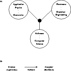
Figure 3.1:
The Multi-Disciplinary (Three-Team) Approach to Computing
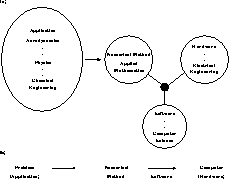
Figure 3.2:
An Alternative (Four-Team) Multi-Disciplinary Approach to Computing
We believe that much of the success (and perhaps also the failures) of
 can be traced to its interdisciplinary nature. In this
spirit, we will provide here a partial integration of the disparate
contributions in this volume with a mathematical framework that links
hardware, software, and applications. In this chapter, we will
describe the principles behind this integration which will then be
amplified and exemplified in the following chapters. This integration
is usually contained in the first introductory section of each
chapter. In Section
3.2
, we define a general methodology for
computation and propose that it be described as mappings between
complex systems. The latter are only loosely
defined but several examples are given in Section
3.3
, while
relevant properties of complex systems are given in
Sections
3.4
through Section
3.6
. Section
3.7
describes mappings between different complex systems and how this
allows one to classify software approaches. Section
3.8
uses
this formalism to state our results and what we mean by ``parallel
computing works.'' In particular, it offers the possibility of a
quantitative approach to such questions as,
can be traced to its interdisciplinary nature. In this
spirit, we will provide here a partial integration of the disparate
contributions in this volume with a mathematical framework that links
hardware, software, and applications. In this chapter, we will
describe the principles behind this integration which will then be
amplified and exemplified in the following chapters. This integration
is usually contained in the first introductory section of each
chapter. In Section
3.2
, we define a general methodology for
computation and propose that it be described as mappings between
complex systems. The latter are only loosely
defined but several examples are given in Section
3.3
, while
relevant properties of complex systems are given in
Sections
3.4
through Section
3.6
. Section
3.7
describes mappings between different complex systems and how this
allows one to classify software approaches. Section
3.8
uses
this formalism to state our results and what we mean by ``parallel
computing works.'' In particular, it offers the possibility of a
quantitative approach to such questions as,
``Which parallel machine is suitable for which problems?''
and
``What software models are suitable for what problems on what machines?''
Next:
The Process of
Up:
3 A Methodology for
Previous:
3 A Methodology for
Guy Robinson
Wed Mar 1 10:19:35 EST 1995
The Process of Computation and ComplexSystems
Next:
Examples of Complex
Up:
3 A Methodology for
Previous:
3.1 Introduction
There is no agreed-upon process behind computation, that is, behind the use of
a computer to solve a particular problem. We have tried to quantify this in
Figures
3.1
(b),
3.2
(b), and
3.3
which show a problem being first numerically formulated and then mapped by
software onto a computer.
Figure 3.3:
An Interdisciplinary Approach to Computing with Computational
Science Shown Shaded
Even if we could get agreement on such an ``underlying'' process, the
definitions of the parts of the process are not precise and correspondingly
the roles of the ``experts'' are poorly defined. This underlies much of the
controversy, and in particular, why we cannot at present or probably ever
be able to define
``The best software methodology for parallel computing.''
How can we agree on a solution (What is the appropriate software?) unless we
can agree on the task it solves?
``What is computation and how can it be broken up into components?''
In other words, what is the underlying process?
In spite of our pessimism that there is any clean, precise answer to
this question, progress can be made with an imperfect process defined
for computation. In the earlier figures, it was stressed that software
could be viewed as mapping problems onto computers. We can elaborate
this as shown in Figure
3.4
, with the solution to a
question pictured as a sequence of idealizations or simplifications
which are finally mapped onto the computer. This process is spelled
out for four examples in Figures
3.5
and
3.6
. In each case, we have tried to indicate possible
labels for components of the process. However, this can only be
approximate. We are not aware of an accepted definition for the
theoretical or computational parts of the process. Again, which parts
are modelling
or simulation? Further, there is only
an approximate division of responsibility among the various
``experts''; for example, between the theoretical physicist and the
computational physicist, or among aerodynamics,
applied mathematics, and computer science. We have also not
illustrated that, in each case, the numerical algorithm is dependent on
the final computer architecture targeted; in particular, the best
parallel algorithm is often different from the best conventional
sequential algorithm.
Figure 3.4:
An Idealized Process of Computation
Figure 3.5:
A Process for Computation in Two Examples in Basic Physics
Simulations
Figure 3.6:
A Process for Computation in Two Examples from Large Scale
System Simulations
We can abstract Figures
3.5
and
3.6
into a sequence
of maps between complex systems  ,
,  .
.
We have anticipated (Chapter
5
) and broken the software into a
high level component (such as a compiler)
and a lower
level one (such as an assembler) which maps a ``virtual computer'' into
the particular machine under consideration. In fact, the software
could have more stages, but two is the most common case for simple
(sequential) computers.
A complex system, as used here, is defined as a collection of fundamental
entities whose static or dynamic properties define a connection scheme
between the entities. Complex systems have a structure or architecture.
For instance, a binary hypercube parallel computer of dimension
d
is
a complex system with  members connected in a hypercube
topology. We can focus in on the node of the hypercube and expand the
node, viewed itself as a complex system, into a collection of memory
hierarchies, caches, registers, CPU., and communication channels. Even
here, we find another ill-defined point with the complex system representing
the computer dependent on the resolution or granularity with which you
view the system. The importance of the architecture of a computer
system
members connected in a hypercube
topology. We can focus in on the node of the hypercube and expand the
node, viewed itself as a complex system, into a collection of memory
hierarchies, caches, registers, CPU., and communication channels. Even
here, we find another ill-defined point with the complex system representing
the computer dependent on the resolution or granularity with which you
view the system. The importance of the architecture of a computer
system  has been recognized for many years. We suggest
that the architecture or structure of the problem is comparably
interesting. Later, we will find that the performance of a particular
problem or machine can be studied in terms of the match (similarity)
between the architectures of the complex systems
has been recognized for many years. We suggest
that the architecture or structure of the problem is comparably
interesting. Later, we will find that the performance of a particular
problem or machine can be studied in terms of the match (similarity)
between the architectures of the complex systems  and
and
 defined in Equation
3.1
. We will find
that the structure of the appropriate parallel software will depend on
the broad features of the (similar) architecture of
defined in Equation
3.1
. We will find
that the structure of the appropriate parallel software will depend on
the broad features of the (similar) architecture of  and
and
 . This can be expected as software maps the two
complex systems into each other.
. This can be expected as software maps the two
complex systems into each other.
At times, we have talked in terms of problem architecture,
but this is ambiguous since it could refer to any of the
complex systems  which can and usually do have
different architectures. Consider the second example of
Figure
3.5
with the computational fluid
dynamics
study of airflow. In the
language of Equation
3.1
:
which can and usually do have
different architectures. Consider the second example of
Figure
3.5
with the computational fluid
dynamics
study of airflow. In the
language of Equation
3.1
:
-
-
 is a (finite) collection of molecules interacting with
long-range Van der Waals and other forces. This interaction defines a
complete interconnect between all members of the complex system
is a (finite) collection of molecules interacting with
long-range Van der Waals and other forces. This interaction defines a
complete interconnect between all members of the complex system  .
.
-
-
 is the infinite degree of freedom continuum with the fundamental
entities as infinitesimal volumes of air connected locally by the partial
differential operator of the Navier Stokes
equation.
is the infinite degree of freedom continuum with the fundamental
entities as infinitesimal volumes of air connected locally by the partial
differential operator of the Navier Stokes
equation.
-
-
 could depend on the particular numerical
formulation used. Multigrid, conjugate gradient
, direct matrix inversion and alternating gradient would have
very different structures in the direct numerical solution of the
Navier Stokes equations. The more radical cellular
automata
approach would be quite different
again.
could depend on the particular numerical
formulation used. Multigrid, conjugate gradient
, direct matrix inversion and alternating gradient would have
very different structures in the direct numerical solution of the
Navier Stokes equations. The more radical cellular
automata
approach would be quite different
again.
-
-
 would depend on the final computer being used
and division between high and low level in software. In the applications
described in this book,
would depend on the final computer being used
and division between high and low level in software. In the applications
described in this book,  would typically be a simple binary hypercube
with
would typically be a simple binary hypercube
with  nodes.
-
-
 would be
  embroidered by the
details of the hardware communication (circuit or packet switching, wormhole
or other routing). Further, as described above, in some analyses we could
look at this complex system in greater resolution and expose the details of
the processor node architecture.
embroidered by the
details of the hardware communication (circuit or packet switching, wormhole
or other routing). Further, as described above, in some analyses we could
look at this complex system in greater resolution and expose the details of
the processor node architecture.
Next:
Examples of Complex
Up:
3 A Methodology for
Previous:
3.1 Introduction
Guy Robinson
Wed Mar 1 10:19:35 EST 1995
Examples of Complex
Systems and TheirSpace-Time Structure
Next:
3.4 The Temporal Properties
Up:
3 A Methodology for
Previous:
The Process of
In the previous section, we showed how the process of computation could be
viewed as mappings between complex systems. As the book progresses, we will
quantify this by providing examples that cover a range of problem
architectures. In the next three sections, we will set up the general
framework and define terms which will be made clearer later on as we see the
explicit problems with their different architectures. The concept of complex
systems may have very general applicability to a
wide range of fields but here we will focus solely on their application to
computation. Thus, our discussion of their properties will only cover
what we have found useful for the task at hand. These properties
are surely more generally applicable, and one can expect that other
ideas will be needed in a general discussion. Section
3.3
gives examples and a basic definition of a complex system and its
associated space-time structure. Section
3.4
defines temporal
properties and, finally, Section
3.5
spatial
structures.
We wish to understand the interesting characteristics or structure of a
complex system. We first introduce the concept of space-time into a general
complex system. As shown in Figure
3.7
, we consider a general
complex system as a
space
, or data domain, that evolves
deterministically or probabilistically with time. Often, the space-time
associated with a given complex system is identical with physical space-time
but sometimes it is not. Let us give some examples.
Figure 3.7:
(a) Synchronous, Loosely Synchronous (Static), and (b)
Asynchronous (Dynamic) Complex Systems with their Space-Time Structure
-
For a computer considered as a complex system, the
space
is the
collection of processing nodes, communication channels and peripherals as
illustrated in Figures 1.1 and 1.2.
Time
is the physical time, but it is
usually quantized, with for instance a unit of
 seconds
for a
seconds
for a  node.
node.
-
An earthquake
can be considered as a physical
complex system (
 ) which is first mapped, by the theoretical
geophysicist who is modelling it, into displacements measured by the
amplitudes of waves as a function of space and time. Here again, the
complex system (
) which is first mapped, by the theoretical
geophysicist who is modelling it, into displacements measured by the
amplitudes of waves as a function of space and time. Here again, the
complex system ( )
space-time
is mapped into physical
space-time. One might Fourier-Transform this picture to obtain a third
complex system (
)
space-time
is mapped into physical
space-time. One might Fourier-Transform this picture to obtain a third
complex system ( ) whose space is now labelled by wave numbers.
-
One might record this earthquake on a collection of
N
strip
recorders. Now the resultant complex system (
 ) is a collection of
N
sheets of paper. The space of
) is a collection of
N
sheets of paper. The space of  consists of the set of sheets and has
N
discrete members. The
time
associated with
consists of the set of sheets and has
N
discrete members. The
time
associated with  is the
extension along the ``long'' (say
x
) direction of each sheet. This complex
system is specified by the recording on the other (
y
) direction as a
function of the
time
defined above. This example illustrates how
mappings between complex systems can mix space and time. This is further
illustrated by the next example, which completes the sequence of complex
systems related to earthquakes.
is the
extension along the ``long'' (say
x
) direction of each sheet. This complex
system is specified by the recording on the other (
y
) direction as a
function of the
time
defined above. This example illustrates how
mappings between complex systems can mix space and time. This is further
illustrated by the next example, which completes the sequence of complex
systems related to earthquakes.
-
Suppose one writes a Fortran program to simulate such an earthquake and
runs it on a conventional single processor workstation. This von Neumann
model of computation has mapped the original complex system
 into one
(
into one
( ) with perhaps one or at best a few elements in its spatial domain
corresponding to the independent functional units on the workstation.
) with perhaps one or at best a few elements in its spatial domain
corresponding to the independent functional units on the workstation.  has mapped the original space-time into a totally temporal complex
system. This could be viewed either as an example of the richness of mappings
allowed between complex systems or as an illustration of the artificial nature
of the sequential computing! Simulation of an earthquake on a parallel
computer more faithfully links the space-time of the problem (
has mapped the original space-time into a totally temporal complex
system. This could be viewed either as an example of the richness of mappings
allowed between complex systems or as an illustration of the artificial nature
of the sequential computing! Simulation of an earthquake on a parallel
computer more faithfully links the space-time of the problem ( ) with that
of the simulation (
) with that
of the simulation ( ).
).
-
The seismic
simulation, mentioned above, could involve
solution of the wave equation

Consider instead the solution of the elliptic partial differential equation

for the electrostatic potential  in the presence of a charge density
 . A simple, albeit usually non-optimal approach to solving
Equation
3.4
, is a Jacobi iteration, which in the special case
of two dimensions and
. A simple, albeit usually non-optimal approach to solving
Equation
3.4
, is a Jacobi iteration, which in the special case
of two dimensions and  involves the iterative procedure

where we assume that integer values of the indices
x
and
y
label the
two-dimensional grid on which Laplace's
equation is to
be solved. The complex system defined by Equation
3.5
has
spatial
domain defined by the  grid and a
temporal
dimension defined by the iteration index
n
. Indeed, the
Jacobi iteration is mathematically related to solving the parabolic
partial differential equation
grid and a
temporal
dimension defined by the iteration index
n
. Indeed, the
Jacobi iteration is mathematically related to solving the parabolic
partial differential equation

where one relates the discretized time
t
to the iteration index
n
. This
equivalence between Equations
3.5
and
3.6
is qualitatively preserved when one compares the solution of
Equations
3.3
and
3.5
. As long as one
views iteration as a temporal structure,
Equations
3.3
and
3.4
can be formulated
numerically with isomorphic complex systems  . This implies
that parallelization issues, both hardware and software, are
essentially identical for both equations.
. This implies
that parallelization issues, both hardware and software, are
essentially identical for both equations.
The above example illustrates the most important form of
parallelism-namely,
data parallelism
. This is produced by
parallel execution of a computational (temporal) algorithm on each
member of a
space
or
data domain
. Data parallelism is
essentially synonymous with either
massive parallelism
or
massive data parallelism
. Spatial domains are usually very large,
with from  to
to  members today; thus exploiting this data
parallelism does lead to massive parallelism.
members today; thus exploiting this data
parallelism does lead to massive parallelism.
-
As a final example, consider a particular simple formulation of the
solution of linear equations,
 with a dense (few zero
elements) matrix
A
.
with a dense (few zero
elements) matrix
A
.

Parallelization of this is covered fully in [
Fox:88a
] and
Chapter
8
of this book. Gaussian elimination
(LU decomposition)
for solving Equation
3.7
involves successive steps where
in the simplest formulation without pivoting,
at step
k
one ``eliminates'' a single variable  where the index
  . At each step
k
, one modifies both
. At each step
k
, one modifies both  and
and 

and  ,
,  are formed from
  ,
,

where one ensures (if no pivoting is employed) that
 when
j>k
. Consider the above procedure as a
complex system. The
spatial
domain is formed by the matrix
A
with a two-dimensional array of values
when
j>k
. Consider the above procedure as a
complex system. The
spatial
domain is formed by the matrix
A
with a two-dimensional array of values  . The time domain
is labelled by the index
k
and so is a discrete space with
n
(number of rows or columns of
A
) members. The space is also discrete
with
. The time domain
is labelled by the index
k
and so is a discrete space with
n
(number of rows or columns of
A
) members. The space is also discrete
with  members.
Next:
3.4 The Temporal Properties
Up:
3 A Methodology for
Previous:
The Process of
Guy Robinson
Wed Mar 1 10:19:35 EST 1995
3.4 The Temporal Properties
of ComplexSystems
Next:
3.5 Spatial Properties of
Up:
3 A Methodology for
Previous:
Examples of Complex
As shown in Equation
3.1
, we will use complex systems to unify
a variety of different concepts including nature and an underlying theory
such as Quantum Chromodynamics;
the
numerical formulation of the theory; the result of expressing this
with various software paradigms and the final computer used in its
simulation. Different disciplines have correctly been built up around
these different complex systems. Correspondingly different terminology
is often used to describe related issues. This is certainly reasonable
for both historical and technical reasons. However, we argue that
understanding the process of computation and answering questions such
as, ``Which parallel computers are good for which problems?''; ``What
problems parallelize?''; and ``What are productive parallel software
paradigms?'' is helped by a terminology which bridges the different
complex systems. We can illustrate this with an anecdote. In a recent
paper, an illustration of particles in the universe was augmented with
a hierarchical set of clusters produced with the algorithm of
Section
12.4
. These clusters are designed to accurately
represent the different length scales and physical clustering of the
clouds of particles. This picture was labelled ``data structure'' but
one computer science referee noted that this was not appropriate.
Indeed, the referee was in one sense correct-we had not displayed a
computer science data structure such as a Fortran array or C structure
defining the linked list
of particles. However,
taking the point of view of the physicist, this picture was precisely
showing the structure of the data and so, the caption was in one
discipline (physics) correct and in another (computer science) false!
We will now define and discuss some general properties and parameters of
complex systems which span the various disciplines involved.
-
For completeness, we define a
complex system
as a collection of members whose extent defines the associated
space
and whose evolution defines the associated
time
. Many
examples of these definitions were given in Section
3.3
.
We will first discuss possible temporal structures for a complex
system. Here, we draw on a computer science classification of computer
architecture. In this context, aspects such as internode topology
refer to the spatial structure of the computer viewed as a complex
system. The control structure of the computer refers to the temporal
behavior of its complex system. In our review of parallel computer
hardware, we have already introduced the concepts of SIMD and MIMD, two
important temporal classes which carry over to general complex
systems. Returning to Figures
3.7
(a) and
3.7
(b), we see complex systems which are
MIMD
(or asynchronous as defined below) in
Figure
3.7
(b) and either SIMD or a restricted form of
MIMD in Figure
3.7
(a) (synchronous or loosely synchronous
in language below). In fact, when we consider the temporal structure
of problems ( in Equation
3.1
), software
(
in Equation
3.1
), software
( ), and hardware (
 in
Equation
3.1
), we will need to further extend this
classification. Here we will briefly define concepts and give the
section number where we discuss and illustrate it more fully.
in
Equation
3.1
), we will need to further extend this
classification. Here we will briefly define concepts and give the
section number where we discuss and illustrate it more fully.
When we consider computer hardware and software systems, we will need to
consider other temporal classes which can be thought of as further
subdivisions of the asynchronous class.
-
Static asynchronous
(or
static
MIMD) systems
consist of fixed members whose interconnect-or in the application to
parallel computers, message traffic-is varying. This translates into
a MIMD software model of static processes interacting with a general
dynamic message-passing system. We have a fixed number of processes
which are spawned and then execute a particular program which remains
unchanged. This leads to the important SPMD (Single Program Multiple
Data) model of computation [Darema:85a;88a].
This is used in all the applications of this book
except those in Chapters
14
,
17
and
18
.
SPMD is the natural implementation of synchronous or loosely
synchronous problems on MIMD distributed-memory parallel computers. In
SPMD, each process runs the same program but operates on different data
sets. In synchronous implementations, the different processes execute
the same instructions at each computer cycle. In loosely synchronous
problems, the processes are at different points of the same program at
each time.
-
Dynamic asynchronous
systems generalize the above example
with processes and messages able to spawn new processes dynamically.
For instance,
reactive
systems are dynamic asynchronous systems
that spawn services as needed in a distributed operating system.
Generally, we define such systems to have both an irregular
time-dependent interconnect and members which can be created and destroyed
at any time.
-
Shared-memory
MIMD complex systems are defined to
represent this model of parallel computer. This special case of an
asynchronous complex system can only be properly described in
Section
13.1
, when we study software and the associated complex
system
 in the notation of Equation
3.1
.
One could include shared-memory systems as examples of
static
MIMD
or
dynamic asynchronous
systems with a particular form
for information to be transferred between processes or processors. In
distributed-memory machines, information is transferred via the
construction of messages; in shared memory
by
memory access instructions. Indeed, the so-called NUMA (non-uniform
memory access) shared-memory machines are implemented in machines like
the Kendall Square as distributed-memory hardware with (from the point
of view of the user) memory access as the communication mechanism.
Uniform memory access (UMA) shared memory machines, such as the
Sequent, do present a rather different computational model. However,
most believe that NUMA machines are the only shared-memory
architectures that scale to large systems, and so in practice scalable
shared-memory architectures are only distinguished from
distributed-memory machines in their mechanism for information
transfer.
in the notation of Equation
3.1
.
One could include shared-memory systems as examples of
static
MIMD
or
dynamic asynchronous
systems with a particular form
for information to be transferred between processes or processors. In
distributed-memory machines, information is transferred via the
construction of messages; in shared memory
by
memory access instructions. Indeed, the so-called NUMA (non-uniform
memory access) shared-memory machines are implemented in machines like
the Kendall Square as distributed-memory hardware with (from the point
of view of the user) memory access as the communication mechanism.
Uniform memory access (UMA) shared memory machines, such as the
Sequent, do present a rather different computational model. However,
most believe that NUMA machines are the only shared-memory
architectures that scale to large systems, and so in practice scalable
shared-memory architectures are only distinguished from
distributed-memory machines in their mechanism for information
transfer.
-
Dataflow
can be considered as a special dynamic
asynchronous complex system describing the dataflow
hardware and/or software model of
 or
or  in
Equation
3.1
. Here, members of the complex system are
dormant until all data needed for their definition is received when
they ``fire'' and evolve according to a predetermined algorithm.
in
Equation
3.1
. Here, members of the complex system are
dormant until all data needed for their definition is received when
they ``fire'' and evolve according to a predetermined algorithm.
In Figure
3.8
, we summarize these temporal classifications
for complex systems, indicating a partial ordering with arrows pointing
to more general architectures. This will become clearer in
Section
3.5
when we discuss software and the relation between
problem and computer. Note that although the language is drawn from
the point of view of computer architecture, the classifications are
important at the problem, software, and hardware level.
Figure 3.8:
Partial Ordering of Temporal (Control) Architectures for a Complex
System
The hardware (computer) architecture naturally divides into SIMD
(synchronous), MIMD (asynchronous), and von Neumann classes. The problem
structures are synchronous, loosely synchronous, or asynchronous. One can
argue that the shared-memory asynchronous architecture is naturally suggested
by software ( ) considerations and in particular by the goal of
efficient parallel execution for sequential software models. For this reason
it becomes an important computer architecture even though it is not a natural
problem (
) considerations and in particular by the goal of
efficient parallel execution for sequential software models. For this reason
it becomes an important computer architecture even though it is not a natural
problem ( ) architecture.
Next:
3.5 Spatial Properties of
Up:
3 A Methodology for
Previous:
Examples of Complex
Guy Robinson
Wed Mar 1 10:19:35 EST 1995
3.5 Spatial Properties of Complex Systems
Next:
3.6 Compound Complex Systems
Up:
3 A Methodology for
Previous:
3.4 The Temporal Properties
Now we switch topics and consider the spatial properties of complex systems.
The
size
N
of the complex system is obviously an important
property. Note that we think of a complex system as a set of
members
with their spatial structure evolving with time. Sometimes,
the time domain has a definite ``size'' but often one can evolve the
system indefinitely in time. However, most complex systems have a
natural spatial size with the spatial domain consisting of
N
members. In the examples of Section
3.3
, the seismic example
had a definite spatial extent and unlimited time domain; on the other
hand, Gaussian elimination
had  spatial members evolving for a fixed number of
n
``time'' steps. As
usual, the value of spatial size
N
will depend on the granularity or
detail with which one looks at the complex system. One could consider
a parallel computer as a complex system constructed as a collection of
transistors with a correspondingly very large value of
spatial members evolving for a fixed number of
n
``time'' steps. As
usual, the value of spatial size
N
will depend on the granularity or
detail with which one looks at the complex system. One could consider
a parallel computer as a complex system constructed as a collection of
transistors with a correspondingly very large value of  but here we will view the processor node as the fundamental entity and
define the spatial size of a parallel computer viewed as a complex
system, by the number
but here we will view the processor node as the fundamental entity and
define the spatial size of a parallel computer viewed as a complex
system, by the number  of processing nodes.
Now is a natural time to define the von Neumann complex system
spatial structure which is relevant, of course, for computer architecture. We
will formally define this to be a system with no spatial extent, i.e.
size  . Of course, a von Neumann node can have a
sophisticated structure if we look at fine enough resolution with multiple
functional units. More precisely, perhaps, we can generalize this complex
system to one where
. Of course, a von Neumann node can have a
sophisticated structure if we look at fine enough resolution with multiple
functional units. More precisely, perhaps, we can generalize this complex
system to one where  is small and will not scale up to large
values.
is small and will not scale up to large
values.
Consider mapping a seismic
simulation with  grid
points onto a parallel machine with
grid
points onto a parallel machine with  processors. An important
parameter is the
grain size
n
of the resultant decomposition. We
can introduce the problem
grain size
processors. An important
parameter is the
grain size
n
of the resultant decomposition. We
can introduce the problem
grain size
 and the computer
grain size
and the computer
grain size
 as the memory contained in each node of the parallel computer. Clearly we
must have,
as the memory contained in each node of the parallel computer. Clearly we
must have,

if we measure memory size in units of seismic grid points. More
interestingly, in Equation
3.10
we will relate the
performance of the parallel implementation of the seismic simulation to
 and other problem and computer characteristics. We find that,
in many cases, the parallel performance only depends on
and other problem and computer characteristics. We find that,
in many cases, the parallel performance only depends on  and
and
 in the combination
  and so
grain size
is a critical parameter in determining the effectiveness
of parallel computers for a particular application.
and so
grain size
is a critical parameter in determining the effectiveness
of parallel computers for a particular application.
The next set of parameters describe the topology or structure of the
spatial domain associated with the complex system. The simplest parameter
of this type is the geometric dimension  of the space. As
reviewed in Chapter
2
, the original hardware and, in fact, software
(see Chapter
5
) exhibited a clear geometric structure for
of the space. As
reviewed in Chapter
2
, the original hardware and, in fact, software
(see Chapter
5
) exhibited a clear geometric structure for
 or
or  . The binary hypercube of dimension
d
had this as its geometric dimension. This was an effective architecture
because it was richer than the topologies of most problems. Thus, consider
mapping a problem of dimension
. The binary hypercube of dimension
d
had this as its geometric dimension. This was an effective architecture
because it was richer than the topologies of most problems. Thus, consider
mapping a problem of dimension  onto a computer of dimension
 . Suppose the software system preserves the spatial structure
of the problem and that
. Suppose the software system preserves the spatial structure
of the problem and that  . Then, one can show
that the parallel computing overhead
f
has a term due to internode
communication that has the form,
. Then, one can show
that the parallel computing overhead
f
has a term due to internode
communication that has the form,

with parallel speedup
S
given by

The communication overhead  depends on the problem
grain size
depends on the problem
grain size
 and computer complex system
  . It also involves
two parameters specifying the parallel hardware performance.
. It also involves
two parameters specifying the parallel hardware performance.
-
 : The typical time required to perform a
generic calculation. For scientific problems, this can be taken as a
floating-point calculation
: The typical time required to perform a
generic calculation. For scientific problems, this can be taken as a
floating-point calculation

-
 : The typical time taken to communicate
a single word between two nodes connected in the hardware topology.
: The typical time taken to communicate
a single word between two nodes connected in the hardware topology.
The definitions of  and
and  are imprecise
above. In particular,
are imprecise
above. In particular,  depends on the nature of node and
can take on very different values depending on the details of the
implementation; floating-point operations are much faster when the
operands are taken from registers than from slower parts of the memory
hierarchy. On systems built from processors like the Intel i860 chip,
these effects can be large;
depends on the nature of node and
can take on very different values depending on the details of the
implementation; floating-point operations are much faster when the
operands are taken from registers than from slower parts of the memory
hierarchy. On systems built from processors like the Intel i860 chip,
these effects can be large;  could be
  from registers (50 MFLOPS) and larger by a factor of ten when the
variables
a,b
are fetched from dynamic RAM. Again, communication
speed
from registers (50 MFLOPS) and larger by a factor of ten when the
variables
a,b
are fetched from dynamic RAM. Again, communication
speed  depends on internode message size (a software
characteristic) and the latency
(startup time) and
bandwidth
of the computer communication subsystem.
depends on internode message size (a software
characteristic) and the latency
(startup time) and
bandwidth
of the computer communication subsystem.
Returning to Equation
3.10
, we really only need to understand
here that the term  indicates that communication
overhead depends on relative performance of the internode communication
system and node (floating-point) processing unit. A real study of
parallel computer performance would require a deeper discussion of the
exact values of
indicates that communication
overhead depends on relative performance of the internode communication
system and node (floating-point) processing unit. A real study of
parallel computer performance would require a deeper discussion of the
exact values of  and
and  . More interesting here is
the dependence
. More interesting here is
the dependence  on the number of
processors
on the number of
processors  and problem
grain size
and problem
grain size
 . As
described above,
grain size
. As
described above,
grain size
 depends on both the problem and the computer. The values of
  and
and  are given by

independent of computer parameters, while if

The results in Equation
3.13
quantify the penalty, in
terms of a value of  that increases with
  , for a
computer architecture that is less rich than the problem
architecture.
An attractive feature of the
hypercube architecture is that
, for a
computer architecture that is less rich than the problem
architecture.
An attractive feature of the
hypercube architecture is that  is large and one is
essentially always in the regime governed by the top line in
Equation
3.13
. Recently, there has been a trend away
from rich topologies like the hypercube towards the view that the node
interconnect should be considered as a routing network or switch to be
implemented in the very best technology. The original MIMD machines
from Intel, nCUBE,
and AMETEK
all used
hypercube topologies, as did the SIMD Connection
Machines
CM-1 and CM-2. The nCUBE-2,
introduced in 1990, still uses a hypercube topology but both it and the
second generation Intel iPSC/2 used a hardware routing that ``hides''
the hypercube connectivity. The latest Intel Paragon and Touchstone
Delta and Symult (ex-Ametek) 2010 use a two-dimensional mesh with
wormhole routing. It is not clear how to incorporate these new node
interconnects into the above picture and further research is needed.
Presumably, we would need to add new complex system properties and
perhaps generalize the definition of dimension
is large and one is
essentially always in the regime governed by the top line in
Equation
3.13
. Recently, there has been a trend away
from rich topologies like the hypercube towards the view that the node
interconnect should be considered as a routing network or switch to be
implemented in the very best technology. The original MIMD machines
from Intel, nCUBE,
and AMETEK
all used
hypercube topologies, as did the SIMD Connection
Machines
CM-1 and CM-2. The nCUBE-2,
introduced in 1990, still uses a hypercube topology but both it and the
second generation Intel iPSC/2 used a hardware routing that ``hides''
the hypercube connectivity. The latest Intel Paragon and Touchstone
Delta and Symult (ex-Ametek) 2010 use a two-dimensional mesh with
wormhole routing. It is not clear how to incorporate these new node
interconnects into the above picture and further research is needed.
Presumably, we would need to add new complex system properties and
perhaps generalize the definition of dimension  as we
will see below is in fact necessary for Equation
3.10
to
be valid for problems whose structure is not geometrically based.
as we
will see below is in fact necessary for Equation
3.10
to
be valid for problems whose structure is not geometrically based.
Returning to Equations
3.10
through
3.12
,
we note that we have not properly defined the correct dimension
 or
or  to use. We have implicitly equated
this with the natural
geometric dimension
but this is not
always correct. This is illustrated by the complex system
to use. We have implicitly equated
this with the natural
geometric dimension
but this is not
always correct. This is illustrated by the complex system  consisting of a set of particles in three dimensions interacting
with a long range force such as gravity or electrostatic charge. The
geometric structure is local with
consisting of a set of particles in three dimensions interacting
with a long range force such as gravity or electrostatic charge. The
geometric structure is local with  but
the complex system structure is quite different; all particles are
connected to all others. As described in Chapter 3 of [
Fox:88a
],
this implies that
but
the complex system structure is quite different; all particles are
connected to all others. As described in Chapter 3 of [
Fox:88a
],
this implies that  whatever the
underlying geometric structure. We define the
system
dimension
whatever the
underlying geometric structure. We define the
system
dimension
 for a general complex
system to reflect the system connectivity. Consider Figure
3.9
which shows a general domain
D
in a complex system. We define the
volume
for a general complex
system to reflect the system connectivity. Consider Figure
3.9
which shows a general domain
D
in a complex system. We define the
volume
 of this domain by the information in it. Mathematically,
 is the computational complexity needed to simulate
D
in isolation.
In a geometric system
is the computational complexity needed to simulate
D
in isolation.
In a geometric system

where
L
is a geometric length scale. The domain
D
is not in general
isolated and is connected to the rest of the complex system. Information
 flows in
D
and again in a geometric system.
flows in
D
and again in a geometric system.  is a surface
effect with
is a surface
effect with

Figure 3.9:
The Information Density and Flow in a General Complex System
with Length Scale
L
If we view the complex system as a graph,  is related to the
number of links of the graph inside
D
and
is related to the
number of links of the graph inside
D
and  is related to the
number of links cut by the surface of
D
. Equations
3.14
and
3.15
are altered in cases like the long-range
force
problem where the complex system
connectivity is no longer geometric. We define the system dimension to
preserve the surface versus volume interpretation of
Equation
3.15
compared to Equation
3.14
.
Thus, generally we define
is related to the
number of links cut by the surface of
D
. Equations
3.14
and
3.15
are altered in cases like the long-range
force
problem where the complex system
connectivity is no longer geometric. We define the system dimension to
preserve the surface versus volume interpretation of
Equation
3.15
compared to Equation
3.14
.
Thus, generally we define

With this definition of
system dimension
 , we will
find that Equations
3.10
through
3.12
essentially hold in general. In particular for the long range force problem,
one finds
, we will
find that Equations
3.10
through
3.12
essentially hold in general. In particular for the long range force problem,
one finds  independent of
  .
.
A very important special type of spatial structure is the case
 when we find the
embarrassingly
parallel
or
spatially
disconnected
complex system. Here there is no connection between
the different members in the spatial domain. Applying this to parallel
computing, we see that if
when we find the
embarrassingly
parallel
or
spatially
disconnected
complex system. Here there is no connection between
the different members in the spatial domain. Applying this to parallel
computing, we see that if  or
or  is
spatially disconnected, then it can be parallelized very straightforwardly.
In particular, any MIMD machine can be used whatever the temporal
structure of the complex system. SIMD machines can only be used to
simulate embarrassingly parallel complex systems which have spatially
disconnected members with
identical
structure.
is
spatially disconnected, then it can be parallelized very straightforwardly.
In particular, any MIMD machine can be used whatever the temporal
structure of the complex system. SIMD machines can only be used to
simulate embarrassingly parallel complex systems which have spatially
disconnected members with
identical
structure.
In Section
13.7
, we extend the analysis of this section to cover
the performance of hierarchical memory
machines. We find that one needs to replace subdomains in space with
those in space-time.
In Chapter
11
, we describe other interesting spatial properties
in terms of a particle analogy. We find system temperature and phase
transitions as one heats and cools the complex system.
Next:
3.6 Compound Complex Systems
Up:
3 A Methodology for
Previous:
3.4 The Temporal Properties
Guy Robinson
Wed Mar 1 10:19:35 EST 1995
3.6 Compound Complex Systems
Next:
3.7 Mapping Complex Systems
Up:
3 A Methodology for
Previous:
3.5 Spatial Properties of
In Sections
3.4
and
3.5
, we discussed basic
characteristics of complex systems. In fact, many ``real world examples''
are a mixture of these fundamental architectures. This is illustrated by
Figure
3.10
, which shows a very conventional computer network
with several different architectures. We cannot only regard each individual
computer as a complex system but the whole network is, of course, a single
complex system as we have defined it. We will term such complex systems
compound
. Note that one often puts together a network of resources to
solve a ``single problem'' and so an analysis of the structure of compound
complex systems is not an academic issue, but of practical importance.
Figure 3.10:
A Heterogeneous Compound Complex System  Corresponding
to a Network of Computers of Disparate Architectures
Corresponding
to a Network of Computers of Disparate Architectures
Figure
3.10
shows a mixture of temporal, synchronous and
asynchronous, and spatial, hypercube, and von Neumann architectures.
We can look at both the architecture of the individual network
components or, taking a higher level view, look at the network itself
with member computers, such as the hypercube in Figure
3.10
,
viewed as ``black boxes.'' In this example, the network is an
asynchronous complex system and this seems quite a common circumstance.
Figure
3.11
shows two compound problems
 coming from the aerospace and battle management fields,
respectively. In each case we link asynchronously problem modules
which are synchronous, loosely synchronous, or asynchronous. We have
found this very common. In scientific and engineering computations,
the basic modules are usually synchronous or loosely synchronous.
These modules have large spatial size and naturally support ``massive
data parallelism.'' Rarely do we find large asynchronous modules;
this is fortunate as such complex systems are difficult to
parallelize. However, in many cases the synchronous or loosely
synchronous program modules are hierarchically combined with an
asynchronous architecture. This is an important way in which the
asynchronous problem architecture
is used
in large scale computations. This is explored in detail in
Chapter
18
. One has come to refer to systems such as those
in Figure
3.10
as
metacomputers
.
Correspondingly, we designate the applications in
Figure
3.11
metaproblems
.
coming from the aerospace and battle management fields,
respectively. In each case we link asynchronously problem modules
which are synchronous, loosely synchronous, or asynchronous. We have
found this very common. In scientific and engineering computations,
the basic modules are usually synchronous or loosely synchronous.
These modules have large spatial size and naturally support ``massive
data parallelism.'' Rarely do we find large asynchronous modules;
this is fortunate as such complex systems are difficult to
parallelize. However, in many cases the synchronous or loosely
synchronous program modules are hierarchically combined with an
asynchronous architecture. This is an important way in which the
asynchronous problem architecture
is used
in large scale computations. This is explored in detail in
Chapter
18
. One has come to refer to systems such as those
in Figure
3.10
as
metacomputers
.
Correspondingly, we designate the applications in
Figure
3.11
metaproblems
.
Figure:
Two Heterogeneous Complex Systems  Corresponding
to: a) the Integrated Design of a New Aircraft, and b) the Integrated
Battle Management Problem Discussed in Chapter
18
Corresponding
to: a) the Integrated Design of a New Aircraft, and b) the Integrated
Battle Management Problem Discussed in Chapter
18
If we combine Figures
3.10
and
3.11
, we can
formulate the process of computation in its most general complicated fashion.
``Map a compound heterogeneous problem onto a compound heterogeneous
computer.''
Next:
3.7 Mapping Complex Systems
Up:
3 A Methodology for
Previous:
3.5 Spatial Properties of
Guy Robinson
Wed Mar 1 10:19:35 EST 1995
3.7 Mapping Complex Systems
Next:
3.8 Parallel Computing Works?
Up:
3 A Methodology for
Previous:
3.6 Compound Complex Systems
Equation
3.1
first stated our approach to computation as a map
between different complex systems. We can quantify this by defining a
partial order on complex systems written

Equation
3.17
states that a complex system
A
can be
mapped to complex system
B
, that is, that
B
has a more general
architecture than
A
. This was already seen in Figure
3.8
and is given in more detail in Figure
3.12
, where we have
represented complex systems in a two-dimensional space labelled by
their spatial and temporal properties. In this notation, we require:

Figure 3.12:
An Illustration of Problem or Computer Architecture Represented
in a Two-dimensional Space. The spatial structure only gives a few
examples.
The requirement that a particular problem parallelize is that

which is shown in Figure
3.13
. We have drawn our space
labelled by complex system properties so that the partial ordering of
Figures
3.8
and
3.12
``flows'' towards the
origin. Roughly, complex systems get more specialized as one either moves
upwards or to the right. We view the three key complex systems,
 ,
,  , and
, and  , as points in the space
represented in Figures
3.12
and
3.13
.
Then Figure
3.13
shows that the computer complex system
, as points in the space
represented in Figures
3.12
and
3.13
.
Then Figure
3.13
shows that the computer complex system
 lies below and to the left of those representing
  and
and  .
.
Let us consider an example. Suppose  (the computer) is a
hypercube of dimension
(the computer) is a
hypercube of dimension  with a MIMD temporal
structure.
Synchronous, loosely
synchronous, or asynchronous problems can be mapped onto this computer
as long as the problem's spatial structure is contained in the
hypercube topology. Thus, we will successfully map a
with a MIMD temporal
structure.
Synchronous, loosely
synchronous, or asynchronous problems can be mapped onto this computer
as long as the problem's spatial structure is contained in the
hypercube topology. Thus, we will successfully map a  two-dimensional mesh.
But what about a
two-dimensional mesh.
But what about a  mesh or
 irregular lattice? The
  mesh only
has nine (spatial) components and insufficient parallelism to exploit
the 64-node computer. The large irregular mesh can be efficiently
mapped onto the hypercube as shown in Chapter
12
. However, one
could support this with a more general computer architecture where
hardware or software routing essentially gives the general node-to-node
communication shown in the bottom left corner of
Figure
3.12
. The hypercube work at Caltech and elsewhere
always used this strategy in mapping complex spatial topologies; the
crystal-router
mechanism in CrOS or Express was a powerful and
efficient software strategy. Some of the early work using
transputers
found difficulties with some spatial
structures
since the language
Occam
only directly supported process-to-process
communication over the physical hardware channels. However, later
general Occam subroutine libraries (communication ``harnesses'')
callable from FORTRAN or C allowed the general point-to-point
(process-to-process) communication model for transputer systems.
mesh only
has nine (spatial) components and insufficient parallelism to exploit
the 64-node computer. The large irregular mesh can be efficiently
mapped onto the hypercube as shown in Chapter
12
. However, one
could support this with a more general computer architecture where
hardware or software routing essentially gives the general node-to-node
communication shown in the bottom left corner of
Figure
3.12
. The hypercube work at Caltech and elsewhere
always used this strategy in mapping complex spatial topologies; the
crystal-router
mechanism in CrOS or Express was a powerful and
efficient software strategy. Some of the early work using
transputers
found difficulties with some spatial
structures
since the language
Occam
only directly supported process-to-process
communication over the physical hardware channels. However, later
general Occam subroutine libraries (communication ``harnesses'')
callable from FORTRAN or C allowed the general point-to-point
(process-to-process) communication model for transputer systems.
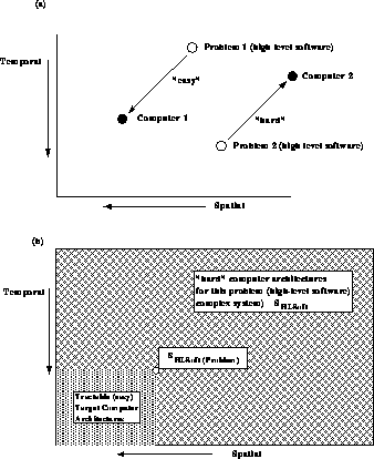
Figure:
Easy and Hard Mappings of Complex Systems  or
or  . We show
complex systems for problems and computers in a space labelled by
spatial and temporal complex system (computer architectures).
Figure
3.12
illustrates possible ordering of
these structures.
. We show
complex systems for problems and computers in a space labelled by
spatial and temporal complex system (computer architectures).
Figure
3.12
illustrates possible ordering of
these structures.
Next:
3.8 Parallel Computing Works?
Up:
3 A Methodology for
Previous:
3.6 Compound Complex Systems
Guy Robinson
Wed Mar 1 10:19:35 EST 1995
3.8 Parallel Computing Works?
Next:
4 Synchronous Applications I
Up:
3 A Methodology for
Previous:
3.7 Mapping Complex Systems
The complex system classification introduced in this chapter allows a
precise formulation of the lessons of current research.
The majority of large scale scientific and engineering computations have
synchronous or loosely synchronous character. Detailed statistics are
given in Section
14.1
but we note that our survey suggests that at
most 10% of applications are asynchronous. The microscopic or macroscopic
temporal synchronization in the synchronous or loosely synchronous problems
ensures natural parallelism without difficult computer hardware or software
synchronization. Thus, we can boldly state that

for these problems. This quantifies our statement that
``Parallel Computing Works,''
where Equation
3.20
should be interpreted in the sense shown in
Figure
3.13
(b).
Roughly, loosely synchronous problems are suitable for MIMD and synchronous
problems for SIMD computers. We can expand Equation
3.20
and
write
The results in Equation
3.21
are given with more details
in Tables
14.1
and
14.2
. The text of this
book is organized so that we begin by studying the simpler synchronous
applications, then give examples first of loosely synchronous and
finally asynchronous and compound problems.
The bold statements in Equations
3.20
and
3.21
become less clear when one considers software and the associated
software complex system  . The parallel software
systems CrOS and its follow-on Express were used in nearly all
our applications. These required explicit user insertion of message
passing, which in many cases is tiresome and unfamiliar. One can argue
that, as shown in Figure
3.14
, we supported a high-level
software environment that reflected the target machine and so could be
effectively mapped on it. Thus, we show
. The parallel software
systems CrOS and its follow-on Express were used in nearly all
our applications. These required explicit user insertion of message
passing, which in many cases is tiresome and unfamiliar. One can argue
that, as shown in Figure
3.14
, we supported a high-level
software environment that reflected the target machine and so could be
effectively mapped on it. Thus, we show  (CrOS) and
 (MIMD) close together on Figure
3.14
. A
more familiar and attractive environment to most users would be a
traditional sequential language like Fortran77. Unfortunately,
(MIMD) close together on Figure
3.14
. A
more familiar and attractive environment to most users would be a
traditional sequential language like Fortran77. Unfortunately,

and so, as shown in Figures
3.13
(a) and
3.14
, it
is highly non-trivial to effectively map existing or new Fortran77
codes onto MIMD or SIMD parallel machines-at least those with
distributed memory. We will touch on this issue in this book in
Sections
13.1
and
13.2
, but it remains an active
research area.
We also discuss
data parallel
languages, such as High Performance
Fortran, in Chapter
13
[
Kennedy:93a
]. This is designed so that

Figure 3.14:
The Dusty Deck Issue in Terms of the Architectures of Problem,
Software, and Computer Complex Systems
We can show this point more graphically if we introduce a quantitative
measure
M
of the difficulty of mapping  . We represent
M
as the difference in heights
h
,
. We represent
M
as the difference in heights
h
,

where we can only perform the map if
M
is positive

Negative values of
M
correspond to difficult cases such as
Equation
3.22
while large positive values of
M
imply a
possible but hard map. Figure
3.15
shows how one can now
picture the process of computation as moving ``downhill'' in the complex
system architecture space.
Figure 3.15:
Two Problems  and Five Computer Architectures
  in the Space-Time Architecture Classification of Complex Systems. An arrow
represents a successful mapping and an ``X'' a mapping that will fail without a
sophisticated compiler.
in the Space-Time Architecture Classification of Complex Systems. An arrow
represents a successful mapping and an ``X'' a mapping that will fail without a
sophisticated compiler.
This formal discussion is illustrated throughout the book by numerous
examples, which show that a wide variety of applications parallelize.
Most of the applications chapters start with a computational analysis
that refers back to the general concepts developed. This is finally
summarized in Chapter
14
, which exemplifies the asynchronous
applications and starts with an overview of the different temporal
problem classes. We build up to this by discussing synchronous
problems in Chapters
4
and
6
; embarrassingly
parallel problems in Chapter
7
; loosely synchronous
problem with increasing degrees of irregularity in Chapters
8
,
9
, and
12
. Compound problem classes-an asynchronous
mixture of loosely synchronous components-are described in
Chapters
17
and
18
. The large missile tracking and
battle management simulation built at JPL (Figure
3.11
b)
and described briefly in Chapter
18
was the major example of
a compound problem
class within C P.
Chapters
17
and
19
indicate that we believe that this
class is extremely important in many ``real-world'' applications that
integrate many diverse functions.
P.
Chapters
17
and
19
indicate that we believe that this
class is extremely important in many ``real-world'' applications that
integrate many diverse functions.
Next:
4 Synchronous Applications I
Up:
3 A Methodology for
Previous:
3.7 Mapping Complex Systems
Guy Robinson
Wed Mar 1 10:19:35 EST 1995
4 Synchronous Applications I
Next:
4.1 QCD and the
Up:
Parallel Computing Works
Previous:
3.8 Parallel Computing Works?
Guy Robinson
Wed Mar 1 10:19:35 EST 1995
4.1 QCD and the Beginning of CP
Next:
4.2 Synchronous Applications
Up:
4 Synchronous Applications I
Previous:
4 Synchronous Applications I
The Caltech Concurrent Computation Project started with QCD,
or
Quantum Chromodynamics,
as its first
application. QCD is discussed in more detail in Sections
4.2
and
4.3
, but here we will put in the historical perspective.
This nostalgic approach is developed in [
Fox:87d
], [
Fox:88oo
]
as well as Chapters
1
and
2
of this book.
We show, in Table
4.1
, fourteen QCD simulations, labelled by
representative physics publications, performed within C P using
parallel machines. This activity started in 1981 with simulations,
using the first four-node 8086-8087-based prototypes of the Cosmic
Cube. These prototypes were quite competitive in performance with the
VAX 11/780 on which we had started (in 1980) our computational physics
program within high energy physics
at
Caltech. The 64-node Cosmic Cube
was used more or
less continuously from October, 1983 to mid-1984 on what was termed by
Caltech, a ``mammoth calculation'' in the press release shown in
Figure
4.2
. This is the modest,
P using
parallel machines. This activity started in 1981 with simulations,
using the first four-node 8086-8087-based prototypes of the Cosmic
Cube. These prototypes were quite competitive in performance with the
VAX 11/780 on which we had started (in 1980) our computational physics
program within high energy physics
at
Caltech. The 64-node Cosmic Cube
was used more or
less continuously from October, 1983 to mid-1984 on what was termed by
Caltech, a ``mammoth calculation'' in the press release shown in
Figure
4.2
. This is the modest,  four-dimensional lattice calculation reported in line 3 of
Table
4.1
. As trumpeted in Figures
4.1
and
4.2
, this was our first major use of parallel machines and
a critical success on which we built our program.
four-dimensional lattice calculation reported in line 3 of
Table
4.1
. As trumpeted in Figures
4.1
and
4.2
, this was our first major use of parallel machines and
a critical success on which we built our program.
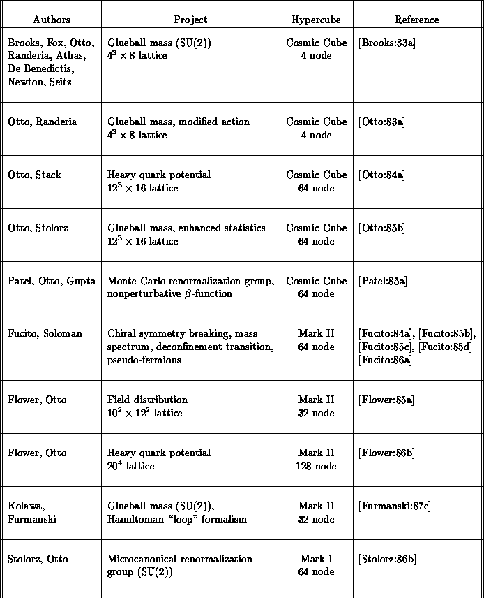
Table 4.1:
Quantum Chromodynamic (QCD) Calculations Within C P
P
Our 1983-1984 calculations totalled some 2,500 hours on the 64-node
Cosmic Cube and successfully competed with 100-hour CDC
Cyber 205 computations that were the state of the art at the time
[
Barkai:84b
], [
Barkai:84c
], [
Bowler:85a
],
[
DeForcrand:85a
]. We used a four-dimensional lattice with  grid points, with eight gluon field values defined on each
of the 110,592 links between grid points. The resultant 884,736
degrees of freedom seem modest today as QCD practitioners contemplate
lattices of order
grid points, with eight gluon field values defined on each
of the 110,592 links between grid points. The resultant 884,736
degrees of freedom seem modest today as QCD practitioners contemplate
lattices of order  simulated on machines of
teraFLOP
performance [
Aoki:91a
]. However, this
lattice was comparable to those used on vector supercomputers at the
time.
simulated on machines of
teraFLOP
performance [
Aoki:91a
]. However, this
lattice was comparable to those used on vector supercomputers at the
time.
A hallmark of this work was the interdisciplinary team building hardware,
software, and parallel application. Further, from the start we stressed
large supercomputer-level simulations where parallelism would make the
greatest initial impact. It was also worth noting that our use of
comparatively high-level software paid off-Otto and Stack were able to
code better algorithms [
Parisi:83a
] than the competing vector
supercomputer teams. The hypercube could be programmed conveniently
without use of microcode or other unproductive environments needed on
some of the other high-performance machines of the time.
Our hypercube calculations used an early C plus message-passing
programming approach which later evolved into the
Express
system
described in the next chapter. Although not as elegant as data-parallel
C and Fortran (discussed in Chapter
13
), our approach was easier
than hand-coded assembly, which was quite common for alternative
high-performance systems of the time.
Figures
4.1
and
4.2
show extracts from
Caltech and newspaper publicity of the time. We were essentially only
a collection of 64 IBM PCs. Was that a good thing (as we thought) or
an indication of our triviality (as a skeptical observer commenting in
Figure
4.1
thought)? 1985 saw the start of a new phase as
conventional supercomputers and availability increased in power and NSF
and DOE allocated many tens of thousands of hours on the
CRAY X-MP
(2, Y-MP) and ETA-10 to QCD simulations. Our
final QCD hypercube calculations in 1989 within C P used a 64-node
JPL Mark IIIfp with approximately
P used a 64-node
JPL Mark IIIfp with approximately  performance. Since
this work, we switched to using the Connection Machine
CM-2, which by 1990 was the commercial standard in the field.
C
performance. Since
this work, we switched to using the Connection Machine
CM-2, which by 1990 was the commercial standard in the field.
C P helped the Los Alamos group of Brickner and Gupta (one of our
early graduates!) to develop the first CM-2 QCD codes, which in 1991
performed at
P helped the Los Alamos group of Brickner and Gupta (one of our
early graduates!) to develop the first CM-2 QCD codes, which in 1991
performed at  on the full size
  CM-2
[
Brickner:91a
], [
Liu:91a
].
CM-2
[
Brickner:91a
], [
Liu:91a
].
Caltech Scientists Develop `Parallel' Computer Model
By LEE DEMBART
Times Science Writer
Caltech scientists have developed a working prototype for a new super
computer that can perform many tasks at once, making possible the
solution of important science and engineering problems that have so
far resisted attack.
The machine is one of the first to make extensive use of parallel
processing, which has been both the dream and the bane of computer
designers for years.
Unlike conventional computers, which perform one step at a time while
the rest of the machine lies idle, parallel computers can do many
things at the same time, holding out the prospect of much greater
computing speed than currently available-at much less cost.
If its designers are right, their experimental device, called the
Cosmic Cube, will open the way for solving problems in
meteorology,
aerodynamics,
high-energy physics, seismic
analysis,
astrophysics
and oil exploration, to name a few.
These problems have been intractable because even the fastest of
today's computers are too slow to process the mountains of data in a
reasonable amount of time.
One of today's fastest computers is the Cray 1, which can do 20
million to 80 million operations a second. But at $5 million, they
are expensive and few scientists have the resources to tie one up
for days or weeks to solve a problem.
``Science and engineering are held up by the lack of super
computers,'' says one of the Caltech inventors, Geoffrey C. Fox, a
theoretical physicist. ``They know how to solve problems that are
larger than current computers allow.''
The experimental device, 5 feet long by 8 inches high by 14 inches
deep, fits on a desk top in a basement laboratory, but it is already
the most powerful computer at Caltech. It cost $80,000 and can do
three million operations a second-about one-tenth the power of a
Cray 1.
Fox and his colleague, Charles L. Seitz, a computer scientist, say
they can expand their device in coming years so that it has 1,000
times the computing power of a Cray.
``Poor old Cray and Cyber (another super computer) don't have much of
a chance of getting any significant increase in speed,'' Fox said.
``Our ultimate machines are expected to be at least 1,000 times faster
than the current fastest computers.''
``We are getting to the point where we are not going to be talking
about these things as fractions of a Cray but as multiples of them,''
Seitz said.
But not everyone in the field is as impressed with Caltech's Cosmic
Cube as its inventors are. The machine is nothing more nor less than
64 standard, off-the-shelf microprocessors wired together, not much
different than the innards of 64 IBM personal computers working as a
unit.
``We are using the same technology used in PCs (personal computers)
and Pacmans,'' Seitz said. The technology is an 8086 microprocessor
capable of doing 1/20th of a million operations a second with 1/8th of
a megabyte of primary storage. Sixty-four of them together will do 3
million operations a second with 8 megabytes of storage.
Currently under development is a single chip that will replace each of
the 64 8-inch-by-14-inch boards. When the chip is ready, Seitz and
Fox say they will be able to string together 10,000 or even 100,000 of
them.
Computer scientists have known how to make such a computer for years
but have thought it too pedestrian to bother with.
``It could have been done many years ago,'' said Jack B. Dennis, a
computer scientist at the Massachusetts Institute of Technology who is
working on a more radical and ambitious approach to parallel
processing than Seitz and Fox. He thinks his approach, called
``dataflow,''
will both speed up computers and expand
their horizons, particularly in the direction of artificial
intelligence
.
Computer scientists dream of getting parallel processors to mimic the
human brain
, which can also do things concurrently.
``There's nothing particularly difficult about putting together 64 of
these processors,'' he said. ``But many people don't see that sort of
machine as on the path to a profitable result.''
What's more, Dennis says, organizing these machines and writing
programs for them have turned out to be sticky problems that have
resisted solution and divided the experts.
``There is considerable debate as to exactly how these large parallel
machines should be programmed,'' Dennis said by telephone from
Cambridge, Mass. ``The 64-processor machine (at Caltech) is, in terms
of cost-performance, far superior to what exists in a Cray 1 or a
Cyber 205 or whatever. The problem is in the programming.''
Fox responds that he has ``an existence proof'' for his machine and
its programs, which is more than Dennis and his colleagues have to
show for their efforts.
The Caltech device is a real, working computer, up and running and
chewing on a real problem in high-energy physics. The ideas on which
it was built may have been around for a while, he agreed, but the
Caltech experiment demonstrates that there is something to be gained
by implementing them.
For all his hopes, Dennis and his colleagues have not yet built a
machine to their specifications. Others who have built parallel
computers have done so on a more modest scale than Caltech's 64
processors. A spokesman for IBM said that the giant computer company
had built a 16-processor machine, and is continuing to explore
parallel processing.
The key insight that made the development of the Caltech computer
possible, Fox said, was that many problems in science are
computationally difficult because they are big, not because they are
necessarily complex.
Because these problems are so large, they can profitably be divided
into 64 parts. Each of the processors in the Caltech machine works on
1/64th of the problem.
Scientists studying the evolution of the universe have to deal with 1
million galaxies. Scientists studying aerodynamics
get
information from thousands of data points in three dimensions.
To hunt for undersea oil, ships tow instruments through the oceans,
gathering data in three dimensions that is then analyzed in two
dimensions because of computer limitations. The Caltech computer
would permit three-dimensional analysis.
``It has to be problems with a lot of concurrency in them,'' Seitz
said. That is, the problem has to be split into parts, and all the
parts have to be analyzed simultaneously.
So the applications of the Caltech computer for commercial uses such
as an airline reservation system would be limited, its inventors
agree.

Figure 4.1:
Caltech Scientists Develop ``Parallel'' Computer Model
[
Dembart:84a
]
CALTECH'S COSMIC CUBE
PERFORMING MAMMOTH CALCULATIONS
Large-scale calculations in basic physics have been successfully run
on the Cosmic Cube, an experimental computer at Caltech that its
developers and users see as the forerunner of supercomputers of the
future. The calculations, whose results are now being published in
articles in scientific journals, show that such computers can deliver
useful computing power at a far lower cost than today's machines.
The first of the calculations was reported in two articles in the June
25 issue of  . In addition,
a second set of calculations related to the first has been submitted
to
. In addition,
a second set of calculations related to the first has been submitted
to  for publication.
The June  articles were:
-``Pure Gauge SU(3) Lattice Theory on an Array of Computers,'' by
Eugene Brooks, Geoffrey Fox, Steve Otto, Paul Stolorz, William Athas,
Erik DeBenedictis, Reese Faucette, and Charles Seitz, all of
Caltech; and John Stack of the University of Illinois at
Urbana-Champaign, and
-``The SU(3) Heavy Quark Potential with High Statistics,'' by Steve
Otto and John Stack.
The Cosmic Cube consists of 64 computer elements, called nodes, that
operate on parts of a problem concurrently. In contrast, most
computers today are so-called von Neumann machines, consisting of a
single processor that operates on a problem sequentially, making
calculations serially.
The calculation reported in the June  took 2,500 hours of the computation time on the
Cosmic Cube. The calculation represents a contribution to the test of
a set of theories called the Quantum Field Theories, which are
mathematical attempts to explain the physical properties of subatomic
particles known as hadrons, which include protons and neutrons.
took 2,500 hours of the computation time on the
Cosmic Cube. The calculation represents a contribution to the test of
a set of theories called the Quantum Field Theories, which are
mathematical attempts to explain the physical properties of subatomic
particles known as hadrons, which include protons and neutrons.
These basic theories represent in a series of equations the behavior
of quarks, the basic constituents of hadrons. Although theorists
believe these equations to be valid, they have never been directly
tested by comparing their predictions with the known properties of
subatomic particles as observed in experiments with particle
accelerators.
The calculations to be published in  probe the properties, such as mass, of the glueballs that are
predicted by theory.
probe the properties, such as mass, of the glueballs that are
predicted by theory.
``The calculations we are reporting are not earth-shaking,'' said Dr.
Fox. ``While they are the best of their type yet done, they represent
but a steppingstone to better calculations of this type.'' According
to Dr. Fox, the scientists calculated the force that exists between
two quarks. This force is carried by gluons, the particles that are
theorized to carry the strong force between quarks. The aim of the
calculation was to determine how the attractive force between quarks
varies with distance. Their results showed that the potential depends
linearly on distance.
``These results indicate that it would take an infinite amount of
energy to separate two quarks, which shows why free quarks are not
seen in nature,'' said Dr. Fox. ``These findings represent a
verification of what most people expected.''
The Cosmic Cube has about one-tenth the power of the most widely used
supercomputer, the Cray-1,
but at one hundredth the cost, about
$80,000. It has about eight times the computing power of the widely
used minicomputer, the VAX 11/780. Physically, the machine occupies
about six cubic feet, making it fit on the average desk, and uses 700
watts of power.
Each of the 64 nodes of the Cosmic Cube has approximately the same
power as a typical microcomputer, consisting of 16-bit Intel 8086 and
8087 processors, with 136K bytes of memory storage. For comparison,
the IBM Personal Computer uses the same family of chips and typically
possesses a similar amount of memory. Each of the Cosmic Cube nodes
executes programs concurrently, and each can send messages to six
other nodes in a communication network based on a six-dimensional
cube, or hypercube. The chips for the Cosmic Cube were donated by
Intel Corporation, and Digital Equipment Corporation contributed
supporting computer hardware. According to Dr. Fox, a full-scale
extension of the Quantum Field Theories to yield the properties of
hadrons would require a computer 1,000 times more powerful than the
Cosmic Cube-or 100 computer projects at Caltech are developing
hardware and software for such advanced machines.

Figure 4.2:
Caltech's Cosmic Cube Performing Mammoth Calculations
[
Meredith:84a
]
It is not surprising that our first hypercube calculations in C P did
not need the full MIMD structure of the machine. This was also a
characteristic of Sandia's pioneering use of the 1024-node nCUBE-[
Gustafson:88a
]. Synchronous applications like QCD are
computationally important and have a simplicity that made them the
natural starting point for our project.
P did
not need the full MIMD structure of the machine. This was also a
characteristic of Sandia's pioneering use of the 1024-node nCUBE-[
Gustafson:88a
]. Synchronous applications like QCD are
computationally important and have a simplicity that made them the
natural starting point for our project.
Next:
4.2 Synchronous Applications
Up:
4 Synchronous Applications I
Previous:
4 Synchronous Applications I
Guy Robinson
Wed Mar 1 10:19:35 EST 1995
4.2 Synchronous Applications
Next:
4.3 Quantum Chromodynamics
Up:
4 Synchronous Applications I
Previous:
4.1 QCD and the
Table
4.2
indicates that 70 percent of our first set of
applications were of the class we call synchronous. As remarked above,
this could be expected in any such early work as these are the problems
with the cleanest structure that are, in general, the simplest to code
and, in particular, the simplest to parallelize. As already defined in
Section
3.4
, synchronous applications
are
characterized by a basic algorithm that consists of a set of operations
which are applied identically in every point in a data set. The
structure of the problem is typically very clear in such applications,
and so the parallel implementation is easier than for the irregular
loosely synchronous and asynchronous cases. Nevertheless, as we will
see, there are many interesting issues in these problems and they
include many very important applications. This is especially true for
academic computations that address fundamental science. These are
often formulated as studies of fundamental microscopic quantities such
as the quark and gluon fundamental particles seen in QCD of
Section
4.3
. Fundamental microscopic entities naturally obey
identical evolution laws and so lead to synchronous problem
architectures. ``Real world problems''-perhaps most extremely
represented by the battle simulations of Chapter
18
in this
book-typically do not involve arrays of identical objects, but rather
the irregular dynamics of several different entities. Thus, we will
find more loosely synchronous and asynchronous problems as we turn from
fundamental science to engineering and industrial or government
applications. We will now discuss the structure of QCD in more detail
to illustrate some general computational features of synchronous
problems.
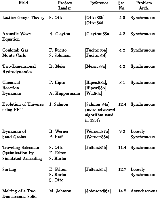
Table 4.2:
The Ten Pioneer Hypercube Applications within C P
P
The applications using the Cosmic Cube
were well
established by 1984 and Table
4.2
lists the ten projects
which were completed in the first year after we started our
interdisciplinary project in the summer of 1983. All but one of these
projects are more or less described in this book, while the other will
be found in [
Fox:88a
]. They covered a reasonable range of
application areas and formed the base on which we first started to
believe that parallel computing works! Figure
4.3
illustrates the regular lattice used in QCD and its decomposition onto
64 nodes. QCD is a four-dimensional theory and all four dimensions can
be decomposed. In our initial 64-node Cosmic Cube calculations, we
used the three-dimensional decompositions shown in
Figure
4.3
with the fourth dimension, as shown in
Figure
4.4
, and internal degrees of freedom stored
sequentially in each node. Figure
4.3
also indicates one
subtlety needed in the parallelization; namely, one needs a so-called
red-black strategy with only half the lattice points updated in each of
the two (``red'' and ``black'') phases. Synchronous applications are
characterized by such a regular spatial domain as shown in
Figure
4.3
and an identical update algorithm for each
lattice point. The update makes use of a Monte Carlo procedure
described in Section
4.3
and in more detail in Chapter 12 of
[
Fox:88a
]. This procedure is not totally synchronous since the
``accept-reject'' mechanism used in the Monte Carlo procedure does not
always terminate at the same step. This is no problem on an MIMD
machine and even makes the problem ``slightly loosely synchronous.''
However, SIMD
machines can also cope with this issue as all
systems (DAP, CM-2, Maspar)
have a feature that allows
processors to either execute the common instruction or ignore it.
Figure 4.3:
A  Problem Lattice Decomposed onto a 64-node Machine
Arranged as a
Problem Lattice Decomposed onto a 64-node Machine
Arranged as a  Machine Lattice. Points labeled X (``red'') or
 (``black'') can be updated at the same time.
Figure:
The 16 time and eight internal gluon degrees of freedom stored
at each point shown in Figure
4.3
Figure
4.5
illustrates the nearest neighbor algorithm used
in QCD and very many problems described by local interactions. We see
that some updates require communication and some don't. In the
message-passing software model used in our hypercube work described in
Chapter
5
, the user is responsible for organizing this
communication with an explicit subroutine call. Our later QCD
calculations and the
spin simulations
of Section
4.4
use the
data-parallel software model on SIMD machines where a compiler
can generate their messaging. Chapter
13
will mention later
projects which are aimed at producing a uniform data parallel Fortran
or C compiler which will generate the correct message structure for
either SIMD or MIMD machines on such regular problems as QCD.
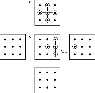
Figure 4.5:
Template of a Local Update Involving No Communication in a) and
the Value to be Communicated in b).
The calculations in Sections
4.3
and
4.4
used a
wide variety of machines, in-house and commercial multicomputers, as well
as the SIMD DAP and CM-2. The spin calculations in Section
4.4
can have very simple degrees of freedom, including that of the binary
``spin'' of the Ising model. These are naturally suited to the
single-bit arithmetic available on the AMT DAP and CM-2. Some of the latest
Monte Carlo algorithms do not use the local algorithms of
Figure
4.4
but exploit the irregular domain structure seen
in materials near a critical point. These new algorithms are much more
efficient but very much more difficult to parallelize-especially on
SIMD machines. They are discussed in Section
12.8
. We also see
a taste of the ``embarrassingly parallel'' problem structure of
Chapter
7
in Section
4.4
. For the Potts
simulation,
we obtained parallelism not from
the data domain (lattice of spins) but from different starting points
for the evolution. This approach, described in more detail in
Section
7.2
, would not be practical for QCD with many degrees
of freedom as one must have enough memory to store the full lattice in
each node of the multicomputer.
Table
4.2
lists the early seismic simulations of the group
led by Clayton, whose C P work is reviewed in Section
18.1
.
These solved the elastic wave equations
using finite
difference
methods as discussed in
Section
3.5
. The equations are iterated with time steps
replacing the Monte Carlo iterations used above. This work is
described in Chapters
5
and
7
of [
Fox:88a
]
and represents methods that can tackle quite practical problems, for
example, predicting the response of complicated geological structures
such as the Los Angeles basin. The two-dimensional hydrodynamics work
of Meier [
Meier:88a
] is computationally similar, using the regular
decomposition and local update of Figures
4.3
and
4.5
. These techniques are now very familiar and may seem
``old-hat.'' However, it is worth noting that, as described in
Chapter
13
, we are only now in 1992 developing the
compiler
technology that will automate these methods
developed ``by-hand'' by our early users. A much more sophisticated
follow-on to these early seismic wave simulations is the ISIS
interactive seismic imaging system described in Chapter
18
.
P work is reviewed in Section
18.1
.
These solved the elastic wave equations
using finite
difference
methods as discussed in
Section
3.5
. The equations are iterated with time steps
replacing the Monte Carlo iterations used above. This work is
described in Chapters
5
and
7
of [
Fox:88a
]
and represents methods that can tackle quite practical problems, for
example, predicting the response of complicated geological structures
such as the Los Angeles basin. The two-dimensional hydrodynamics work
of Meier [
Meier:88a
] is computationally similar, using the regular
decomposition and local update of Figures
4.3
and
4.5
. These techniques are now very familiar and may seem
``old-hat.'' However, it is worth noting that, as described in
Chapter
13
, we are only now in 1992 developing the
compiler
technology that will automate these methods
developed ``by-hand'' by our early users. A much more sophisticated
follow-on to these early seismic wave simulations is the ISIS
interactive seismic imaging system described in Chapter
18
.
Chapter 9 of [
Fox:88a
] explains the well-known synchronous
implementation of long-range particle dynamics.
This algorithm was not used directly in any large C P
application as we implemented the much more efficient cluster
algorithms described in Sections
12.4
,
12.5
, and
12.8
. The initial investigation of the vortex method of
Section
12.5
used the
P
application as we implemented the much more efficient cluster
algorithms described in Sections
12.4
,
12.5
, and
12.8
. The initial investigation of the vortex method of
Section
12.5
used the  method [
Harstad:87a
]. We
also showed a parallel database used in Kolawa's thesis on how a
semi-analytic approach to QCD could be analyzed identically with the
long-range force
problem
[Kolawa:86b;88a]. As explained in [
Fox:88a
],
one can use the long-range force algorithm in any case where the
calculation involves a set of
N
points with observables requiring
functions of every pair of which there are
method [
Harstad:87a
]. We
also showed a parallel database used in Kolawa's thesis on how a
semi-analytic approach to QCD could be analyzed identically with the
long-range force
problem
[Kolawa:86b;88a]. As explained in [
Fox:88a
],
one can use the long-range force algorithm in any case where the
calculation involves a set of
N
points with observables requiring
functions of every pair of which there are  . In the language of
Chapter
3
, this problem has a system dimension
of one, whatever its geometrical dimension. This is
illustrated in Figures
4.6
and
4.7
, which
represent
. In the language of
Chapter
3
, this problem has a system dimension
of one, whatever its geometrical dimension. This is
illustrated in Figures
4.6
and
4.7
, which
represent  in the form of Equations
3.10
and
3.13
. We find
in the form of Equations
3.10
and
3.13
. We find 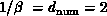 for the
simple two-dimensional decompositions described for the Clayton and
Meier applications for Table
4.2
. We increase range of
R
``interaction'' in Figure
4.7
(a),(b)-defined
formally by
for the
simple two-dimensional decompositions described for the Clayton and
Meier applications for Table
4.2
. We increase range of
R
``interaction'' in Figure
4.7
(a),(b)-defined
formally by

from small (nearest neighbor)
R
to  , the long-range force.
As shown in Figure
4.7
(a),(b),
, the long-range force.
As shown in Figure
4.7
(a),(b),  decreases as
R
increases with the limiting form
decreases as
R
increases with the limiting form  independently of
  for
for  . Noederlinger
[
Lorenz:87a
] and Theiler [Theiler:87a;87b]
used such a ``long-range'' algorithm for
calculating the correlation dimension
of a
chaotic dynamical system. This measures the essential number of
degrees of freedom for a complex system which in this case was a time
series
becoming a plasma. The correction function
involved studying histograms of
. Noederlinger
[
Lorenz:87a
] and Theiler [Theiler:87a;87b]
used such a ``long-range'' algorithm for
calculating the correlation dimension
of a
chaotic dynamical system. This measures the essential number of
degrees of freedom for a complex system which in this case was a time
series
becoming a plasma. The correction function
involved studying histograms of  over the data points
  at time
  .
.
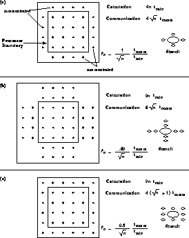
Figure 4.6:
Some Examples of Communication Overhead as a Function of Increasing
Range of Interaction
R
.
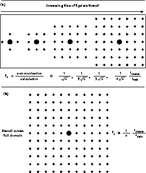
Figure 4.7:
General Form of Communication Overhead for (a) Increasing and
(b) Infinite Range
R
Fucito and Solomon [Fucito:85b;85f]
studied a simple Coulomb gas which naturally had a long-range force.
However, this was a Monte Carlo calculation that was implemented
efficiently by an ingenious algorithm that cannot directly use the
analysis of the particle dynamics (time-stepped) case shown in
Figure
4.7
. Monte Carlo is typically harder to
parallelize than time evolution, where all ``particles'' can be evolved in
time together. However, Monte Carlo updates can only proceed
simultaneously if they involve disjoint particle sets. This implies
the red-black ordering
of
Figure
4.5
and the requiring of a difficult asynchronous
algorithm in the irregular melting problem of Section
14.2
.
Johnson's application was technically the hardest in our list of
pioneers in Table
4.2
.
Finally, Section
4.5
uses cellular automata
ideas that lead to a synchronous architecture to grain
dynamics, which, if implemented directly as in Section
9.2
, would
be naturally loosely synchronous. This illustrates that the problem
architecture depends on the particular numerical approach.
Next:
4.3 Quantum Chromodynamics
Up:
4 Synchronous Applications I
Previous:
4.1 QCD and the
Guy Robinson
Wed Mar 1 10:19:35 EST 1995
4.3 Quantum Chromodynamics
Next:
4.3.1 Introduction
Up:
4 Synchronous Applications I
Previous:
4.2 Synchronous Applications
Other References
HPFA Applications and Paradigms
Guy Robinson
Wed Mar 1 10:19:35 EST 1995
4.3.1 Introduction
Next:
4.3.2 Monte Carlo
Up:
4.3 Quantum Chromodynamics
Previous:
4.3 Quantum Chromodynamics
Quantum chromodynamics
(QCD)
is the proposed theory of the so-called strong
interactions that bind quarks and gluons together to form hadrons-the
constituents of nuclear matter such as the proton and neutron. It also
mediates the forces between hadrons and thus controls the formation of
nuclei. The fundamental properties of QCD cannot be directly tested,
but a wealth of indirect evidence supports this theory. The problem is
that QCD is a nonlinear theory that is not analytically solvable. For
the equivalent quantum field theories of weaker forces such as
electromagnetism, approximations using perturbation expansions in the
interaction strength give very accurate results. However, since the
QCD interaction is so strong, perturbative approximations often fail.
Consequently, few precise predictions can be made from the theory.
This led to the introduction of a non-perturbative approximation based
on discretizing four-dimensional space-time onto a lattice of points,
giving a theory called lattice QCD, which can be simulated on a
computer.
Most of the work on lattice QCD has been directed towards deriving the
masses (and other properties) of the large number of hadrons, which have
been found in experiments using high energy particle accelerators.
This would provide hard evidence for QCD as the theory of the strong
force. Other calculations have also been performed; in particular,
the properties of QCD at finite (i.e., non-zero) temperature and/or
density have been determined. These calculations model the conditions
of matter in the early stages of the evolution of the universe, just
after the Big Bang. Lattice calculations of other quantum field
theories, such as the theory of the weak nuclear force, have also been
performed. For example, numerical calculations have given estimates
for the mass of the Higgs boson, which is currently the Holy Grail of
experimental high energy physics,
and one of
the motivating factors for the construction of the, now cancelled,
$10 billion Superconducting Supercollider.
One of the major problems in solving lattice QCD on a computer is that
the simulation of the quark interactions requires the computation of a
large, highly non-local matrix determinant,
which is
extremely compute-intensive. We will discuss methods for calculating
this determinant later. For the moment, however, we note that, physically,
the determinant arises from the dynamics of the quarks. The simplest
way to proceed is thus to ignore the quark dynamics and work in the
so-called quenched approximation, with only gluonic degrees of
freedom. This should be a reasonable approximation, at least for heavy
quarks. However, even solving this approximate theory requires
enormous computing power. Current state-of-the-art quenched QCD
calculations are performed on lattices of size  , which
involves the numerical solution of a 21,233,664 dimensional integral.
The only way of solving such an integral is by Monte Carlo
methods.
, which
involves the numerical solution of a 21,233,664 dimensional integral.
The only way of solving such an integral is by Monte Carlo
methods.
Next:
4.3.2 Monte Carlo
Up:
4.3 Quantum Chromodynamics
Previous:
4.3 Quantum Chromodynamics
Guy Robinson
Wed Mar 1 10:19:35 EST 1995
4.3.2 Monte Carlo
Next:
4.3.3 QCD
Up:
4.3 Quantum Chromodynamics
Previous:
4.3.1 Introduction
In order to explain the computations for QCD, we use the Feynman path
integral
formalism [
Feynman:65a
]. For any
field theory described by a Lagrangian density  , the dynamics of the
fields
, the dynamics of the
fields  are determined through the action functional

In this language, the measurement of a physical observable represented by an
operator  is given as the expectation value

where the partition function
Z
is

In these expressions, the integral  indicates a sum over all possible
configurations of the field
indicates a sum over all possible
configurations of the field  . A typical observable would be a product
of fields
. A typical observable would be a product
of fields  , which says how the fluctuations in the
field are correlated, and in turn, tells us something about the particles
that can propagate from point
x
to point
y
. The appropriate correlation
functions give us, for example, the masses of the various particles in the
theory. Thus, to evaluate almost any quantity in field theories like QCD,
one must simply evaluate the corresponding path integral. The catch is that
the integrals range are over an infinite-dimensional space.
, which says how the fluctuations in the
field are correlated, and in turn, tells us something about the particles
that can propagate from point
x
to point
y
. The appropriate correlation
functions give us, for example, the masses of the various particles in the
theory. Thus, to evaluate almost any quantity in field theories like QCD,
one must simply evaluate the corresponding path integral. The catch is that
the integrals range are over an infinite-dimensional space.
To put the field theory onto a computer, we begin by discretizing space and
time into a lattice of points. Then the functional
integral is simply defined as the product of the
integrals over the fields at every site of the lattice  :
:

Restricting space and time to a finite box, we end up with a finite (but
very large) number of ordinary integrals, something we might imagine doing
directly on a computer. However, the high dimensionality of these
integrals renders conventional mesh techniques impractical. Fortunately, the
presence of the exponential  means that the integrand is sharply
peaked in one region of configuration space. Hence, we resort to a
statistical treatment and use Monte Carlo type algorithms to sample the
important parts of the integration region [
Binder:86a
].
means that the integrand is sharply
peaked in one region of configuration space. Hence, we resort to a
statistical treatment and use Monte Carlo type algorithms to sample the
important parts of the integration region [
Binder:86a
].
Monte Carlo algorithms typically begin with some initial
configuration of fields, and then make pseudorandom changes on the fields
such that the ultimate probability
P
of generating a particular field
configuration  is proportional to the Boltzmann factor,

where  is the action associated with the given configuration.
There are several ways to implement such a scheme, but for many theories the
simple Metropolis
algorithm [
Metropolis:53a
]
is effective. In this algorithm, a new configuration
is the action associated with the given configuration.
There are several ways to implement such a scheme, but for many theories the
simple Metropolis
algorithm [
Metropolis:53a
]
is effective. In this algorithm, a new configuration  is generated by
updating a single variable in the old configuration
is generated by
updating a single variable in the old configuration  and calculating
the change in action (or energy)
and calculating
the change in action (or energy)

If  , the change is accepted; if
  , the change
is accepted with probability
, the change
is accepted with probability  . In practice, this is done
by generating a pseudorandom number
r
in the
interval [0,1] with uniform probability distribution, and accepting the
change if
. In practice, this is done
by generating a pseudorandom number
r
in the
interval [0,1] with uniform probability distribution, and accepting the
change if  . This is guaranteed to generate the
correct (Boltzmann) distribution of configurations, provided ``detailed
balance''
is satisfied. That condition means
that the probability of proposing the change
. This is guaranteed to generate the
correct (Boltzmann) distribution of configurations, provided ``detailed
balance''
is satisfied. That condition means
that the probability of proposing the change  is
the same as that of proposing the reverse process
is
the same as that of proposing the reverse process
 . In practice, this is true if we never
simultaneously update two fields which interact directly via the
action. Note that this constraint has important ramifications for
parallel computers as we shall see below.
. In practice, this is true if we never
simultaneously update two fields which interact directly via the
action. Note that this constraint has important ramifications for
parallel computers as we shall see below.
Whichever method one chooses to generate field configurations, one updates
the fields for some equilibration time of
E
steps, and then calculates the
expectation value of  in Equation
4.3
from the next
T
configurations as
in Equation
4.3
from the next
T
configurations as

The statistical error in Monte Carlo behaves as  , where
N
is
the number of statistically independent configurations.
, where
N
is
the number of statistically independent configurations.  , where
 is known as the autocorrelation time. This autocorrelation time can
easily be large, and most of the computer time is spent in generating effectively
independent configurations. The operator measurements then become a small
overhead on the whole calculation.
is known as the autocorrelation time. This autocorrelation time can
easily be large, and most of the computer time is spent in generating effectively
independent configurations. The operator measurements then become a small
overhead on the whole calculation.
Next:
4.3.3 QCD
Up:
4.3 Quantum Chromodynamics
Previous:
4.3.1 Introduction
Guy Robinson
Wed Mar 1 10:19:35 EST 1995
4.3.3 QCD
Next:
4.3.4 Lattice QCD
Up:
4.3 Quantum Chromodynamics
Previous:
4.3.2 Monte Carlo
QCD describes the interactions between quarks in high energy physics.
Currently, we know of five types (referred to as ``flavors'') of
quark: up, down, strange, charm, and bottom; and expect one more
(top) to show up soon. In addition to having a ``flavor,'' quarks can
carry one of three possible charges known as ``color'' (this has
nothing to do with color in the macroscopic world!); hence, quantum
chromo
dynamics. The strong color force is mediated by
particles called gluons, just as photons mediate the electromagnetic
force. Unlike photons, though, gluons themselves carry a color charge
and, therefore, interact with one another. This makes QCD a
nonlinear theory, which is impossible to solve analytically.
Therefore, we turn to the computer for numerical solutions.
QCD is an example of a ``gauge theory.'' These are quantum field
theories that have a local symmetry described by a symmetry (or gauge)
group. Gauge theories
are ubiquitous in
elementary particle physics: The electromagnetic interaction
between electrons and photons is described by
quantum electrodynamics
(QED) based on the gauge group U(1); the strong force between quarks
and gluons is believed to be explained by QCD based on the group
SU(3); and there is a unified description of the weak and
electromagnetic
interactions in terms of the
gauge group  . The strength of these interactions
is measured by a coupling constant. This coupling constant is small
for QED, so very precise analytical calculations can be performed using
perturbation theory, and these agree extremely well with experiment.
However, for QCD, the coupling appears to increase with distance (which
is why we never see an isolated quark, since they are always bound
together by the strength of the coupling between them). Perturbative
calculations are therefore only possible at short distances (or large
energies). In order to solve QCD at longer distances, Wilson
[
Wilson:74a
] introduced lattice gauge theory,
in which the space-time continuum is discretized and a discrete version
of the gauge theory is derived which keeps the gauge symmetry intact.
This discretization onto a lattice, which is typically hypercubic,
gives a nonperturbative approximation to the theory that is
successively improvable by increasing the lattice size and decreasing
the lattice spacing, and provides a simple and natural way of
regulating the divergences which plague perturbative approximations.
It also makes the gauge theory amenable to numerical simulation by
computer.
. The strength of these interactions
is measured by a coupling constant. This coupling constant is small
for QED, so very precise analytical calculations can be performed using
perturbation theory, and these agree extremely well with experiment.
However, for QCD, the coupling appears to increase with distance (which
is why we never see an isolated quark, since they are always bound
together by the strength of the coupling between them). Perturbative
calculations are therefore only possible at short distances (or large
energies). In order to solve QCD at longer distances, Wilson
[
Wilson:74a
] introduced lattice gauge theory,
in which the space-time continuum is discretized and a discrete version
of the gauge theory is derived which keeps the gauge symmetry intact.
This discretization onto a lattice, which is typically hypercubic,
gives a nonperturbative approximation to the theory that is
successively improvable by increasing the lattice size and decreasing
the lattice spacing, and provides a simple and natural way of
regulating the divergences which plague perturbative approximations.
It also makes the gauge theory amenable to numerical simulation by
computer.
Next:
4.3.4 Lattice QCD
Up:
4.3 Quantum Chromodynamics
Previous:
4.3.2 Monte Carlo
Guy Robinson
Wed Mar 1 10:19:35 EST 1995
4.3.4 Lattice QCD
Next:
4.3.5 Concurrent QCD Machines
Up:
4.3 Quantum Chromodynamics
Previous:
4.3.3 QCD
To put QCD on a computer, we proceed as follows [
Wilson:74a
],
[
Creutz:83a
]. The four-dimensional
space-time continuum is replaced by a four-dimensional hypercubic periodic
lattice of size  , with the
quarks living on the sites and the gluons living on the links of the lattice.
, with the
quarks living on the sites and the gluons living on the links of the lattice.
 is the spatial and
  is the temporal extent of the lattice. The
lattice has a finite spacing
a
. The gluons are represented by
is the temporal extent of the lattice. The
lattice has a finite spacing
a
. The gluons are represented by
 complex SU(3) matrices associated with each link in the
lattice. The
3
in SU(3) reflects the fact that there are three colors of
quarks, and SU means that the matrices are unitary with unit determinant
(i.e., ``special unitary''). This link matrix describes how the color
of a quark changes as it moves from one site to the next. For example, as a
quark is transported along a link of the lattice it can change its color
from, say, red to green; hence, a red quark at one end of the link can
exchange colors with a green quark at the other end. The action functional
for the purely gluonic part of QCD is
complex SU(3) matrices associated with each link in the
lattice. The
3
in SU(3) reflects the fact that there are three colors of
quarks, and SU means that the matrices are unitary with unit determinant
(i.e., ``special unitary''). This link matrix describes how the color
of a quark changes as it moves from one site to the next. For example, as a
quark is transported along a link of the lattice it can change its color
from, say, red to green; hence, a red quark at one end of the link can
exchange colors with a green quark at the other end. The action functional
for the purely gluonic part of QCD is

where  is a coupling constant and

is the product of link matrices around an elementary square or plaquette on
the lattice-see Figure
4.8
. Essentially all of the time in
QCD simulations of gluons is spent multiplying these SU(3) matrices
together. The main component of this is the  kernel, which
most supercomputers can do very efficiently. As the action involves
interactions around plaquettes, in order to satisfy detailed
balance
we can update only half the links in any one
dimension simultaneously, as shown in Figure
4.9
(in two dimensions
for simplicity). The partition function for full-lattice QCD including quarks
is
kernel, which
most supercomputers can do very efficiently. As the action involves
interactions around plaquettes, in order to satisfy detailed
balance
we can update only half the links in any one
dimension simultaneously, as shown in Figure
4.9
(in two dimensions
for simplicity). The partition function for full-lattice QCD including quarks
is

where  is a large sparse matrix
the
size of the lattice squared. Unfortunately, since the quark or fermion
variables
is a large sparse matrix
the
size of the lattice squared. Unfortunately, since the quark or fermion
variables  are anticommuting Grassmann numbers, there is no
simple representation for them on the computer. Instead, they must be
integrated out, leaving a highly non-local fermion determinant:
are anticommuting Grassmann numbers, there is no
simple representation for them on the computer. Instead, they must be
integrated out, leaving a highly non-local fermion determinant:

This is the basic integral one wants to evaluate numerically.
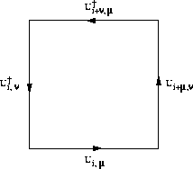
Figure 4.8:
A Lattice Plaquette
Figure 4.9:
Updating the Lattice
The biggest stumbling block preventing large QCD simulations with
quarks is the presence of the determinant  in the
partition function. There have been many proposals for dealing with the
determinant. The first algorithms tried to compute the change in the
determinant when a single link variable was updated [
Weingarten:81a
].
This turned out to be prohibitively expensive. So instead, the approximate
method of pseudo-fermions [
Fucito:81a
] was used.
Today, however, the preferred approach is the so-called Hybrid Monte
Carlo algorithm [
Duane:87a
], which is exact.
The basic idea is to invent some dynamics for the variables in the system in
order to evolve the whole system forward in (simulation) time, and then do a
Metropolis accept/reject for the entire evolution on the basis of the total
energy change. The great advantage is that the whole system is updated in
one fell swoop. The disadvantage is that if the dynamics are not correct,
the acceptance will be very small. Fortunately (and this is one of very few
fortuitous happenings where fermions are concerned), good dynamics can be
found: the Hybrid algorithm [
Duane:85a
]. This is a neat combination
of the deterministic microcanonical method [
Callaway:83a
],
[
Polonyi:83a
] and the stochastic Langevin method [
Parisi:81a
],
[
Batrouni:85a
], which yields a quickly evolving, ergodic algorithm for
both gauge fields and fermions. The computational kernel of this algorithm
is the repeated solution of systems of equations of the form
in the
partition function. There have been many proposals for dealing with the
determinant. The first algorithms tried to compute the change in the
determinant when a single link variable was updated [
Weingarten:81a
].
This turned out to be prohibitively expensive. So instead, the approximate
method of pseudo-fermions [
Fucito:81a
] was used.
Today, however, the preferred approach is the so-called Hybrid Monte
Carlo algorithm [
Duane:87a
], which is exact.
The basic idea is to invent some dynamics for the variables in the system in
order to evolve the whole system forward in (simulation) time, and then do a
Metropolis accept/reject for the entire evolution on the basis of the total
energy change. The great advantage is that the whole system is updated in
one fell swoop. The disadvantage is that if the dynamics are not correct,
the acceptance will be very small. Fortunately (and this is one of very few
fortuitous happenings where fermions are concerned), good dynamics can be
found: the Hybrid algorithm [
Duane:85a
]. This is a neat combination
of the deterministic microcanonical method [
Callaway:83a
],
[
Polonyi:83a
] and the stochastic Langevin method [
Parisi:81a
],
[
Batrouni:85a
], which yields a quickly evolving, ergodic algorithm for
both gauge fields and fermions. The computational kernel of this algorithm
is the repeated solution of systems of equations of the form

where  and
and  are vectors that live on the sites of the
lattice. To solve these equations, one typically uses a conjugate
gradient
algorithm or one of its cousins,
since the fermion matrix
are vectors that live on the sites of the
lattice. To solve these equations, one typically uses a conjugate
gradient
algorithm or one of its cousins,
since the fermion matrix  is sparse. For more
details, see [
Gupta:88a
]. Such iterative matrix algorithms have
as their basic component the
is sparse. For more
details, see [
Gupta:88a
]. Such iterative matrix algorithms have
as their basic component the  kernel, so again
computers which do this efficiently will run QCD well.
kernel, so again
computers which do this efficiently will run QCD well.
Next:
4.3.5 Concurrent QCD Machines
Up:
4.3 Quantum Chromodynamics
Previous:
4.3.3 QCD
Guy Robinson
Wed Mar 1 10:19:35 EST 1995
4.3.5 Concurrent QCD Machines
Next:
4.3.6 QCD on the
Up:
4.3 Quantum Chromodynamics
Previous:
4.3.4 Lattice QCD
Lattice QCD is truly a ``grand challenge'' computing problem. It has
been estimated that it will take on the order of a
TeraFLOP-year
of dedicated computing to obtain
believable results for the hadron mass spectrum in the quenched
approximation, and adding dynamical fermions will involve many orders
of magnitude more operations. Where is the computer power needed for
QCD going to come from? Today, the biggest resources of computer time
for research are the conventional supercomputers at the NSF and DOE
centers. These centers are continually expanding their support for
lattice gauge theory, but it may not be long before they are overtaken
by several dedicated efforts involving concurrent computers. It is a
revealing fact that the development of most high-performance parallel
computers-the Caltech Cosmic Cube,
the Columbia
Machine, IBM's GF11, APE in Rome, the Fermilab Machine and the PAX
machines in Japan-was actually motivated by the desire to simulate
lattice QCD [
Christ:91a
], [
Weingarten:92a
].
As described already, Caltech built the first hypercube computer, the
Cosmic Cube
or Mark I, in 1983. It had 64 nodes,
each of which was an Intel 8086/87 microprocessor with  of
memory, giving a total of about
of
memory, giving a total of about  (measured for QCD).
This was quickly upgraded to the Mark II hypercube with faster chips,
twice the memory per node, and twice the number of nodes in 1984. Then,
QCD was run on the last internal Caltech hypercube, the 128-node
Mark IIIfp
(built by JPL), at
(measured for QCD).
This was quickly upgraded to the Mark II hypercube with faster chips,
twice the memory per node, and twice the number of nodes in 1984. Then,
QCD was run on the last internal Caltech hypercube, the 128-node
Mark IIIfp
(built by JPL), at  sustained [
Ding:90b
]. Each node of the Mark IIIfp hypercube
contains two Motorola 68020 microprocessors, one for communication and
the other for calculation, with the latter supplemented by one 68881
co-processor and a 32-bit Weitek floating point processor.
sustained [
Ding:90b
]. Each node of the Mark IIIfp hypercube
contains two Motorola 68020 microprocessors, one for communication and
the other for calculation, with the latter supplemented by one 68881
co-processor and a 32-bit Weitek floating point processor.
Norman Christ and Anthony Terrano built their first parallel computer
for doing lattice QCD calculations at Columbia in 1984
[
Christ:84a
]. It had 16 nodes, each of which was an Intel
80286/87 microprocessor, plus a TRW 22-bit floating point processor
with  of memory, giving a total peak performance of
  . This was improved in 1987 using Weitek rather than TRW
chips so that 64 nodes gave
. This was improved in 1987 using Weitek rather than TRW
chips so that 64 nodes gave  peak. In 1989, the
Columbia group finished building their third machine: a 256-node,
peak. In 1989, the
Columbia group finished building their third machine: a 256-node,
 , lattice QCD computer [
Christ:90a
].
, lattice QCD computer [
Christ:90a
].
QCDPAX is the latest in the line of PAX (Parallel Array eXperiment)
machines developed at the University of Tsukuba in Japan. The
architecture is very similar to that of the Columbia machine. It is a
MIMD machine configured as a two-dimensional periodic array of nodes,
and each node includes a Motorola 68020 microprocessor and a 32-bit
vector floating-point unit. Its peak performance is similar to that
of the Columbia machine; however, it achieves only half the
floating-point utilization for QCD code [
Iwasaki:91a
].
Don Weingarten initiated the GF11 project in 1984 at IBM. The GF11 is a SIMD
machine comprising 576 Weitek floating point processors, each performing at
 to give the total
  peak implied by the name.
Preliminary results for this project are given in
[Weingarten:90a;92a].
peak implied by the name.
Preliminary results for this project are given in
[Weingarten:90a;92a].
The APE (Array Processor with
Emulator) computer is basically a collection of 3081/E processors (which were
developed by CERN and SLAC for use in high energy experimental physics) with
Weitek floating-point processors attached. However, these floating-point
processors are attached in a special way-each node has four multipliers and
four adders, in order to optimize the  calculations, which
form the major component of all lattice QCD programs. This means that each
node has a peak performance of
calculations, which
form the major component of all lattice QCD programs. This means that each
node has a peak performance of  . The first small
machine-Apetto-was completed in 1986 and had four nodes yielding a peak
performance of
. The first small
machine-Apetto-was completed in 1986 and had four nodes yielding a peak
performance of  . Currently, they have a second generation
of this machine with
. Currently, they have a second generation
of this machine with  peak from 16 nodes. By 1993, the APE
collaboration hopes to have completed the
peak from 16 nodes. By 1993, the APE
collaboration hopes to have completed the  2048-node
``Apecento,'' or APE-100, based on specialized VLSI
chips
that are software compatible with the original APE [
Avico:89a
],
[
Battista:92a
]. The APE-100 is a SIMD machine with the
architecture based on a three-dimensional cubic mesh of nodes.
Currently, a 128-node machine is running with a peak performance of
2048-node
``Apecento,'' or APE-100, based on specialized VLSI
chips
that are software compatible with the original APE [
Avico:89a
],
[
Battista:92a
]. The APE-100 is a SIMD machine with the
architecture based on a three-dimensional cubic mesh of nodes.
Currently, a 128-node machine is running with a peak performance of
 .
.
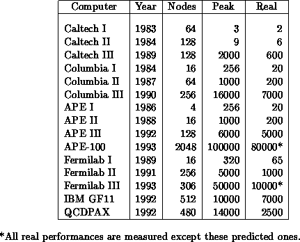
Table 4.3:
Peak and Real Performances in MFLOPS of ``Homebrew'' QCD
Machines
Not to be outdone, Fermilab has also used its high energy experimental
physics emulators to construct a lattice QCD machine called ACPMAPS.
This is a MIMD machine, using a Weitek floating-point chip set on each
node. A 16-node machine, with a peak rate of  , was
finished in 1989. A 256-node machine, arranged as a
, was
finished in 1989. A 256-node machine, arranged as a  hypercube
of crates, with eight nodes communicating through a crossbar in each
crate, was completed in 1991 [
Fischler:92a
]. It has a peak rate
of
hypercube
of crates, with eight nodes communicating through a crossbar in each
crate, was completed in 1991 [
Fischler:92a
]. It has a peak rate
of  , and a sustained rate of about
  for
QCD. An upgrade of ACPMAPS is planned, with the number of nodes being
increased and the present processors being replaced with two Intel
i860 chips per node, giving a peak performance of
for
QCD. An upgrade of ACPMAPS is planned, with the number of nodes being
increased and the present processors being replaced with two Intel
i860 chips per node, giving a peak performance of  per node. These performance figures are summarized in
Table
4.3
. (The ``real'' performances are the actual
performances obtained on QCD codes.)
per node. These performance figures are summarized in
Table
4.3
. (The ``real'' performances are the actual
performances obtained on QCD codes.)
Major calculations have also been performed on commercial SIMD
machines, first on the ICL Distributed Array Processor (DAP) at
Edinburgh University during the period from 1982 to 1987 [
Wallace:84a
],
and now on the TMC Connection Machine
(CM-2); and on commercial distributed memory MIMD machines like the
nCUBE hypercube and Intel Touchstone Delta machines at Caltech.
Currently, the Connection Machine is the most powerful commercial QCD
machine available, running full QCD at a sustained rate of
approximately  on a
on a  CM-2
[
Baillie:89e
], [
Brickner:91b
]. However, simulations have
recently been performed at a rate of
CM-2
[
Baillie:89e
], [
Brickner:91b
]. However, simulations have
recently been performed at a rate of  on the
experimental Intel Touchstone Delta at Caltech. This is a MIMD machine
made up of 528 Intel i860 processors connected in a two-dimensional
mesh, with a peak performance of
on the
experimental Intel Touchstone Delta at Caltech. This is a MIMD machine
made up of 528 Intel i860 processors connected in a two-dimensional
mesh, with a peak performance of  for 32-bit
arithmetic. These results compare favorably with performances on
traditional (vector) supercomputers. Highly optimized QCD code runs at
about
for 32-bit
arithmetic. These results compare favorably with performances on
traditional (vector) supercomputers. Highly optimized QCD code runs at
about  per processor on a CRAY Y-MP,
or
per processor on a CRAY Y-MP,
or
 on a fully configured eight-processor machine.
The generation of commercial parallel supercomputers, represented by the
CM-5 and the Intel Paragon, have a peak performance of over  . There was a proposal for the development of a
TeraFLOPS
parallel supercomputer for QCD and other numerically
intensive simulations [
Christ:91a
], [
Aoki:91a
]. The goal was
to build a
. There was a proposal for the development of a
TeraFLOPS
parallel supercomputer for QCD and other numerically
intensive simulations [
Christ:91a
], [
Aoki:91a
]. The goal was
to build a  machine based on the CM-5 architecture in
collaboration with Thinking Machines Corporation, which would be ready
by 1995 at a cost of around $40 million.
machine based on the CM-5 architecture in
collaboration with Thinking Machines Corporation, which would be ready
by 1995 at a cost of around $40 million.
It is interesting to note that when the various groups began building their
``home-brew'' QCD machines, it was clear they would outperform all
commercial (traditional) supercomputers; however, now that commercial
parallel supercomputers have come of age [
Fox:89n
], the situation is not
so obvious. To emphasize this, we describe QCD calculations on both the
home grown Caltech hypercube and on the commercially available Connection
Machine.
Next:
4.3.6 QCD on the
Up:
4.3 Quantum Chromodynamics
Previous:
4.3.4 Lattice QCD
Guy Robinson
Wed Mar 1 10:19:35 EST 1995
4.3.6 QCD on the Caltech Hypercubes
Next:
4.3.7 QCD on the
Up:
4.3 Quantum Chromodynamics
Previous:
4.3.5 Concurrent QCD Machines
To make good use of MIMD distributed-memory machines like hypercubes, one
should employ domain decomposition. That is, the domain of the problem
should be divided into subdomains of equal size, one for each processor in
the hypercube; and communication routines should be written to take care of
data transfer across the processor boundaries. Thus, for a lattice
calculation, the
N
sites are distributed among the  processors
using a decomposition that ensures that processors assigned to adjacent
subdomains are directly linked by a communication channel in the hypercube
topology. Each processor then independently works through its subdomain of
processors
using a decomposition that ensures that processors assigned to adjacent
subdomains are directly linked by a communication channel in the hypercube
topology. Each processor then independently works through its subdomain of
 sites, updating each one in turn, and only communicating with
neighboring processors when doing boundary sites. This communication
enforces ``loose synchronization,''
which
stops any one processor from racing ahead of the others. Load
balancing is achieved with equal-size domains. If the nodes contain at
least two sites of the lattice, all the nodes can update in parallel,
satisfying detailed balance,
since loose
synchronicity guarantees that all nodes will be doing black, then red
sites alternately.
sites, updating each one in turn, and only communicating with
neighboring processors when doing boundary sites. This communication
enforces ``loose synchronization,''
which
stops any one processor from racing ahead of the others. Load
balancing is achieved with equal-size domains. If the nodes contain at
least two sites of the lattice, all the nodes can update in parallel,
satisfying detailed balance,
since loose
synchronicity guarantees that all nodes will be doing black, then red
sites alternately.
The characteristic timescale of the communication,  , corresponds
roughly to the time taken to transfer a single
, corresponds
roughly to the time taken to transfer a single  matrix from one node to
its neighbor. Similarly, we can characterize the calculational part of the
algorithm by a timescale,
matrix from one node to
its neighbor. Similarly, we can characterize the calculational part of the
algorithm by a timescale,  , which is roughly the time taken to
multiply together two
, which is roughly the time taken to
multiply together two  matrices. For all hypercubes built
without
floating-point accelerator chips,
matrices. For all hypercubes built
without
floating-point accelerator chips,  and, hence,
QCD simulations are extremely ``efficient,'' where efficiency
and, hence,
QCD simulations are extremely ``efficient,'' where efficiency  (Equations
3.10
and
3.11
) is defined by
the relation
(Equations
3.10
and
3.11
) is defined by
the relation

where  is the time taken for
k
processors to perform the given
calculation. Typically, such calculations have efficiencies in the range
is the time taken for
k
processors to perform the given
calculation. Typically, such calculations have efficiencies in the range
 , which means they are ideally suited to this type of
computation since doubling the number of processors nearly halves the
total computational time required for solution. However, as we shall see
(for the Mark IIIfp hypercube, for example), the picture changes dramatically
when fast floating-point chips are used; then
, which means they are ideally suited to this type of
computation since doubling the number of processors nearly halves the
total computational time required for solution. However, as we shall see
(for the Mark IIIfp hypercube, for example), the picture changes dramatically
when fast floating-point chips are used; then  and
one must take some care in coding to obtain maximum performance.
and
one must take some care in coding to obtain maximum performance.
Rather than describe every calculation done on the Caltech hypercubes,
we shall concentrate on one calculation that has been done several times
as the machine evolved-the heavy quark potential
calculation (``heavy'' because the quenched approximation is used).
QCD provides an explanation of why quarks are confined inside hadrons, since
lattice calculations reveal that the inter-quark potential rises linearly as
the separation between the quarks increases. Thus, the attractive force
(the derivative of the potential) is independent of the separation,
unlike other forces, which usually decrease rapidly with distance. This
force, called the ``string tension,'' is carried by the gluons, which form a
kind of ``string'' between the quarks. On the other hand, at short distances,
quarks and gluons are
``asymptotically free'' and behave like electrons and photons, interacting
via a Coulomb-like force. Thus, the quark potential
V
is written as

where
R
is the separation of the quarks,  is the coefficient of the
Coulombic potential and
is the coefficient of the
Coulombic potential and  is the string tension. In fitting
experimental charmonium data to this Coulomb plus linear potential, Eichten
et al. [
Eichten:80a
] estimated that
is the string tension. In fitting
experimental charmonium data to this Coulomb plus linear potential, Eichten
et al. [
Eichten:80a
] estimated that  and
and
 =0.18GeV
 . Thus, a goal of the lattice calculations is to
reproduce these numbers. Enroute to this goal, it is necessary to show that
the numbers from the lattice are ``scaling,'' that is, if one calculates a
physical observable on lattices with different spacings then one gets the
same answer. This means that the artifacts due to the finiteness of the
lattice spacing have disappeared and continuum physics can be extracted.
. Thus, a goal of the lattice calculations is to
reproduce these numbers. Enroute to this goal, it is necessary to show that
the numbers from the lattice are ``scaling,'' that is, if one calculates a
physical observable on lattices with different spacings then one gets the
same answer. This means that the artifacts due to the finiteness of the
lattice spacing have disappeared and continuum physics can be extracted.
The first heavy quark potential calculation using a Caltech hypercube was
performed on the 64-node Mark I in 1984 on a  lattice with
 ranging from
  to
to  [
Otto:84a
]. The value of
[
Otto:84a
]. The value of
 was found to be
  and the string tension (converting to
the dimensionless ratio)
and the string tension (converting to
the dimensionless ratio)  . The numbers
are quite a bit off from the charmonium data but the string tension did
appear to be scaling, albeit in the narrow window
. The numbers
are quite a bit off from the charmonium data but the string tension did
appear to be scaling, albeit in the narrow window  .
.
The next time around, in 1986, the 128-node Mark II hypercube was used on a
 lattice with
  [
Flower:86b
]. The
dimensionless string tension decreased somewhat to 83, but clear violations
of scaling were observed: The lattice was still too coarse to see continuum
physics.
[
Flower:86b
]. The
dimensionless string tension decreased somewhat to 83, but clear violations
of scaling were observed: The lattice was still too coarse to see continuum
physics.
Therefore, the last (1989) calculation using the Caltech/JPL 32-node
Mark IIIfp hypercube concentrated on one  value,
  , and
investigated different lattice sizes:
, and
investigated different lattice sizes:  ,
,  ,
,  ,
,  [
Ding:90b
]. Scaling was not
investigated; however, the values of
[
Ding:90b
]. Scaling was not
investigated; however, the values of  and
and
 , that is,
  = 0.15GeV
 ,
compare favorably with the charmonium data. This work is based on
about 1300 CPU hours on the 32-node Mark IIIfp hypercube, which has a
performance of roughly twice a CRAY X-MP
processor. The
whole 128-node machine performs at
,
compare favorably with the charmonium data. This work is based on
about 1300 CPU hours on the 32-node Mark IIIfp hypercube, which has a
performance of roughly twice a CRAY X-MP
processor. The
whole 128-node machine performs at  . As each node
runs at
. As each node
runs at  , this corresponds to a speedup of 100, and
hence, an efficiency of 78 percent. These figures are for the most
highly optimized code. The original version of the code written in C
ran on the Motorola chips at
, this corresponds to a speedup of 100, and
hence, an efficiency of 78 percent. These figures are for the most
highly optimized code. The original version of the code written in C
ran on the Motorola chips at  and on the Weitek
chips at
and on the Weitek
chips at  . The communication time, which is roughly
the same for both, is less than a 2 percent overhead for the former but
nearly 30 percent for the latter. When the computationally intensive
parts of the calculation are written in assembly code for the Weitek,
this overhead becomes almost 50 percent. This
. The communication time, which is roughly
the same for both, is less than a 2 percent overhead for the former but
nearly 30 percent for the latter. When the computationally intensive
parts of the calculation are written in assembly code for the Weitek,
this overhead becomes almost 50 percent. This  of
communication, shown in lines two and three in Table
4.4
, is
dominated by the hardware/software message startup overhead
(latency),
because for the Mark IIIfp the node-to-node
communication time,
of
communication, shown in lines two and three in Table
4.4
, is
dominated by the hardware/software message startup overhead
(latency),
because for the Mark IIIfp the node-to-node
communication time,  , is given by

where
W
is the number of words transmitted. To speed up the
communication, we update all even (or odd) links (eight in our case) in
each node, allowing us to transfer eight matrix products at a time,
instead of just sending one in each message. This reduces the  by a factor of

to  . On all hypercubes with fast floating-point
chips-and on most hypercubes without these chips for less
computationally intensive codes-such ``vectorization'' of
communication is often important. In Figure
4.10
, the
speedups for many different lattice sizes are shown. For the largest
lattice size, the speedup is 100 on the 128-node machine. The speedup
is almost linear in number of nodes. As the total lattice volume
increases, the speedup increases, because the ratio of
calculation/communication increases. For more information on this
performance analysis,
see [
Ding:90c
].
. On all hypercubes with fast floating-point
chips-and on most hypercubes without these chips for less
computationally intensive codes-such ``vectorization'' of
communication is often important. In Figure
4.10
, the
speedups for many different lattice sizes are shown. For the largest
lattice size, the speedup is 100 on the 128-node machine. The speedup
is almost linear in number of nodes. As the total lattice volume
increases, the speedup increases, because the ratio of
calculation/communication increases. For more information on this
performance analysis,
see [
Ding:90c
].
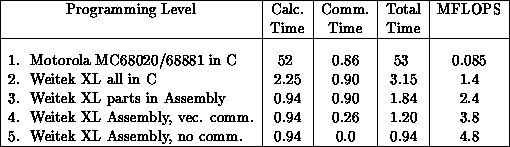
Table 4.4:
Link Update Time (msec) on Mark IIIfp Node for Various Levels
of Programming
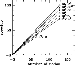
Figure 4.10:
Speedups for QCD on the Mark IIIfp
Next:
4.3.7 QCD on the
Up:
4.3 Quantum Chromodynamics
Previous:
4.3.5 Concurrent QCD Machines
Guy Robinson
Wed Mar 1 10:19:35 EST 1995
4.3.7 QCD on the Connection Machine
Next:
4.3.8 Status and Prospects
Up:
4.3 Quantum Chromodynamics
Previous:
4.3.6 QCD on the
The Connection Machine
Model CM-2 is also
very well suited for large scale simulations of QCD. The CM-2 is a
distributed-memory, single-instruction, multiple-data (SIMD), massively
parallel processor comprising up to 65536 ( ) processors
[Hillis:85a;87a]. Each processor
consists of an arithmetic-logic unit (ALU),
) processors
[Hillis:85a;87a]. Each processor
consists of an arithmetic-logic unit (ALU),  or
or  of random-access memory (RAM), and a router interface to
perform communications among the processors. There are 16 processors
and a router per custom VLSI
chip, with the chips
interconnected as a 12-dimensional hypercube. Communications among
processors within a chip work essentially like a crossbar
interconnect. The router can do general communications, but only local
communication is required for QCD, so we use the fast nearest-neighbor
communication software called NEWS. The processors deal with one bit
at a time. Therefore, the ALU can compute any two Boolean functions as
output from three inputs, and all datapaths are one bit wide. In the
current version of the Connection Machine (the CM-2), groups of 32
processors (two chips) share a 32-bit (or 64-bit) Weitek floating-point
chip, and a transposer chip, which changes 32 bits stored bit-serially
within 32 processors into 32 32-bit words for the Weitek, and vice
versa.
of random-access memory (RAM), and a router interface to
perform communications among the processors. There are 16 processors
and a router per custom VLSI
chip, with the chips
interconnected as a 12-dimensional hypercube. Communications among
processors within a chip work essentially like a crossbar
interconnect. The router can do general communications, but only local
communication is required for QCD, so we use the fast nearest-neighbor
communication software called NEWS. The processors deal with one bit
at a time. Therefore, the ALU can compute any two Boolean functions as
output from three inputs, and all datapaths are one bit wide. In the
current version of the Connection Machine (the CM-2), groups of 32
processors (two chips) share a 32-bit (or 64-bit) Weitek floating-point
chip, and a transposer chip, which changes 32 bits stored bit-serially
within 32 processors into 32 32-bit words for the Weitek, and vice
versa.
The high-level languages on the CM, such as *Lisp and CM-Fortran,
compile into an assembly language called Parallel Instruction Set
(Paris). Paris regards the  bit-serial processors as the
fundamental units in the machine. However, floating-point computations
are not very efficient in the Paris model. This is because in Paris,
32-bit floating-point numbers are stored ``fieldwise''; that is,
successive bits of the word are stored at successive memory locations
of each processor's memory. However, 32 processors share one Weitek
chip, which deals with words stored ``slicewise''-that is, across the
processors, one bit in each. Therefore, to do a floating-point
operation, Paris loads in the fieldwise operands, transposes them
slicewise for the Weitek (using the transposer chip), does the
operation, and transposes the slicewise result back to fieldwise for
memory storage. Moreover, every operation in Paris is an
atomic
process; that is, two operands are brought from
memory and one result is stored back to memory, so no use is made of
the Weitek registers for intermediate results. Hence, to improve the
performance of the Weiteks, a new assembly language called CM
Instruction Set (CMIS) has been written, which models the local
architectural features much better. In fact, CMIS ignores the
bit-serial processors and thinks of the machine in terms of the Weitek
chips. Thus, data can be stored slicewise, eliminating all the
transposing back and forth. CMIS allows effective use of the Weitek
registers, creating a memory hierarchy, which, combined with the
internal buses of the Weiteks, offers increased
bandwidth
for data motion.
bit-serial processors as the
fundamental units in the machine. However, floating-point computations
are not very efficient in the Paris model. This is because in Paris,
32-bit floating-point numbers are stored ``fieldwise''; that is,
successive bits of the word are stored at successive memory locations
of each processor's memory. However, 32 processors share one Weitek
chip, which deals with words stored ``slicewise''-that is, across the
processors, one bit in each. Therefore, to do a floating-point
operation, Paris loads in the fieldwise operands, transposes them
slicewise for the Weitek (using the transposer chip), does the
operation, and transposes the slicewise result back to fieldwise for
memory storage. Moreover, every operation in Paris is an
atomic
process; that is, two operands are brought from
memory and one result is stored back to memory, so no use is made of
the Weitek registers for intermediate results. Hence, to improve the
performance of the Weiteks, a new assembly language called CM
Instruction Set (CMIS) has been written, which models the local
architectural features much better. In fact, CMIS ignores the
bit-serial processors and thinks of the machine in terms of the Weitek
chips. Thus, data can be stored slicewise, eliminating all the
transposing back and forth. CMIS allows effective use of the Weitek
registers, creating a memory hierarchy, which, combined with the
internal buses of the Weiteks, offers increased
bandwidth
for data motion.
When the arithmetic part of the program is rewritten in CMIS (just as
on the Mark IIIfp when it was rewritten in assembly code), the
communications become a bottleneck. Therefore, we need also to speed
up the communication part of the code. On the CM-2, this is done using
the ``bi-directional multi-wire NEWS'' system. As explained above, the
CM chips (each containing 16 processors) are interconnected in a
12-dimensional hypercube. However, since there are two CM chips for
each Weitek floating-point chip, the floating-point hardware is
effectively wired together as an 11-dimensional hypercube, with two
wires in each direction. This makes it feasible to do simultaneous
communications in both directions of all four space-time directions in
QCD-bidirectional multiwire NEWS-thereby reducing the
communication time by a factor of eight. Moreover, the data
rearrangement necessary to make use of this multiwire NEWS further
speeds up the CMIS part of the code by a factor of two.
In 1990-1992, the Connection Machine
was
the most powerful commercial QCD machine available: the ``Los Alamos
collaboration'' ran full QCD at a sustained rate of  on a
on a  CM-2 [
Brickner:91a
]. As was the case for the
Mark IIIfp hypercube, in order to obtain this performance, one must
resort to writing assembly code for the Weitek chips
and
for
the communication. Our original code, written entirely in the CM-2
version of *Lisp, achieved around
CM-2 [
Brickner:91a
]. As was the case for the
Mark IIIfp hypercube, in order to obtain this performance, one must
resort to writing assembly code for the Weitek chips
and
for
the communication. Our original code, written entirely in the CM-2
version of *Lisp, achieved around  [
Baillie:89e
].
As shown in Table
4.5
, this code spends 34 percent of its
time doing communication. When we rewrote the most computationally
intensive part in the assembly language CMIS, this rose to 54 percent.
Then when we also made use of ``multi-wire NEWS'' (to reduce the
communication time by a factor of eight), it fell to 30 percent. The
Intel Delta and Paragon, as well as Thinking Machines CM-5, passed the
CM-2 performance levels in 1993, but here optimization is not yet
complete [
Gupta:93a
].
[
Baillie:89e
].
As shown in Table
4.5
, this code spends 34 percent of its
time doing communication. When we rewrote the most computationally
intensive part in the assembly language CMIS, this rose to 54 percent.
Then when we also made use of ``multi-wire NEWS'' (to reduce the
communication time by a factor of eight), it fell to 30 percent. The
Intel Delta and Paragon, as well as Thinking Machines CM-5, passed the
CM-2 performance levels in 1993, but here optimization is not yet
complete [
Gupta:93a
].
Table 4.5:
Fermion Update Time (sec) on  Connection Machine for
Various Levels of Programming
Connection Machine for
Various Levels of Programming
Next:
4.3.8 Status and Prospects
Up:
4.3 Quantum Chromodynamics
Previous:
4.3.6 QCD on the
Guy Robinson
Wed Mar 1 10:19:35 EST 1995
4.3.8 Status and Prospects
Next:
4.4 Spin Models
Up:
4.3 Quantum Chromodynamics
Previous:
4.3.7 QCD on the
The status of lattice QCD may be summed up as: under way. Already there
have been some nice results in the context of the quenched approximation, but
the lattices are still too coarse and too small to give definitive results.
Results for full QCD are going to take orders of magnitude more computer
time, but we now have an algorithm-Hybrid Monte Carlo-which puts real
simulations within reach.
When will the computer power be sufficient? In Figure
4.11
, we
plot the horsepower of various QCD machines as a function of the year they
started to produce physics results. The performance plotted in this case is
the real sustained rate on actual QCD codes. The surprising fact is that the
rate of increase is very close to exponential, yielding a factor of 10 every
two years! On the same plot, we show our estimate of the computer power
needed to redo correct quenched calculations on a  lattice. This
estimate is also a function of time, due to algorithm improvements.
lattice. This
estimate is also a function of time, due to algorithm improvements.
Figure 4.11:
MFLOPS for QCD Calculations
Extrapolating these trends, we see the outlook for lattice QCD is rather bright.
Reasonable results for the phenomenologically interesting physical
observables should be available within the quenched approximation in the
mid-1990s. With the same computer power, we will be able to redo today's
quenched calculations using dynamic fermions (but still on today's size of
lattice). This will tell us how reliable the quenched approximation is.
Finally, results for the full theory with dynamical fermions on a  lattice should follow early in the next century (!), when computers are two
or three orders of magnitude more powerful.
lattice should follow early in the next century (!), when computers are two
or three orders of magnitude more powerful.
Guy Robinson
Wed Mar 1 10:19:35 EST 1995
4.4 Spin Models
Next:
4.4.1 Introduction
Up:
4 Synchronous Applications I
Previous:
4.3.8 Status and Prospects
Other References
HPFA Applications and Paradigms
Guy Robinson
Wed Mar 1 10:19:35 EST 1995
4.4.1 Introduction
Next:
4.4.2 Ising Model
Up:
4.4 Spin Models
Previous:
4.4 Spin Models
Spin models
are simple statistical models of real
systems, such as magnets,
which exhibit the same
behavior and hence provide an understanding of the physical mechanisms
involved. Despite their apparent simplicity, most of these models are
not exactly soluble by present theoretical methods. Hence, computer
simulation is used. Usually, one is interested in the behavior of the
system at a phase transition;
the computer
simulation reveals where the phase boundaries are, what the phases on
either side are, and how the properties of the system change across the
phase transition. There are two varieties of spins: discrete or
continuous valued. In both cases, the spin variables are put on the
sites of the lattice and only interact with their nearest neighbors.
The partition function for a spin model is

with the action being of the form

where  denotes nearest neighbors,
  is the spin
at site
i
, and
is the spin
at site
i
, and  is a coupling parameter which is proportional
to the interaction strength and inversely proportional to the
temperature. A great deal of work has been done over the years in
finding good algorithms for computer simulations of spin models;
recently some new, much better, algorithms have been discovered. These
so-called cluster algorithms are described in detail in
Section
12.6
. Here, we shall describe results obtained from
using them to perform large-scale Monte Carlo simulations of several
spin models-both discrete and continuous.
is a coupling parameter which is proportional
to the interaction strength and inversely proportional to the
temperature. A great deal of work has been done over the years in
finding good algorithms for computer simulations of spin models;
recently some new, much better, algorithms have been discovered. These
so-called cluster algorithms are described in detail in
Section
12.6
. Here, we shall describe results obtained from
using them to perform large-scale Monte Carlo simulations of several
spin models-both discrete and continuous.
Guy Robinson
Wed Mar 1 10:19:35 EST 1995
4.4.2 Ising Model
Next:
4.4.3 Potts Model
Up:
4.4 Spin Models
Previous:
4.4.1 Introduction
The Ising model
is the simplest model for
ferromagnetism
that predicts phase transitions
and critical phenomena. The spins are discrete and have only two
possible states. This model, introduced by Lenz in 1920
[
Lenz:20a
], was solved in one dimension by Ising in 1925
[
Ising:25a
], and in two dimensions by Onsager in 1944
[
Onsager:44a
]. However, it has not been solved analytically in
three dimensions, so Monte Carlo computer simulation methods have been
one of the methods used to obtain numerical solutions. One of the best
available techniques for this is the Monte Carlo Renormalization
Group
(MCRG) method
[
Wilson:80a
], [
Swendsen:79a
]. The Ising model exhibits a
second-order phase transition in
d=3
dimensions at a critical
temperature  . As
T
approaches
. As
T
approaches  , the correlation length
 diverges as a power law with critical exponent
 :
:

and the
pair correlation function  at
at  falls off to zero with
distance
r
as a power law defining the critical
exponent
falls off to zero with
distance
r
as a power law defining the critical
exponent
 :
:

 ,
,  and
and  determine
the critical behavior of the 3-D Ising model and it is their values we
wish to determine using MCRG.
determine
the critical behavior of the 3-D Ising model and it is their values we
wish to determine using MCRG.
In 1984, this was done by Pawley, Swendsen, Wallace and Wilson
[
Pawley:84a
] in Edinburgh on the ICL DAP computer with high statistics.
They ran on four lattice sizes- ,
,  ,
,  and
and  -measuring
seven even and six odd spin operators. We are essentially repeating their
calculation on the new AMT DAP computer. Why should we do this? First, to
investigate finite size effects-we have run on the biggest lattice used by
Edinburgh,
-measuring
seven even and six odd spin operators. We are essentially repeating their
calculation on the new AMT DAP computer. Why should we do this? First, to
investigate finite size effects-we have run on the biggest lattice used by
Edinburgh,  , and on a bigger one,
  . Second, to investigate
truncation effects-qualitatively the more operators we measure for MCRG,
the better, so we have included 53 even and 46 odd operators. Third, we are
making use of the new cluster-updating algorithm due to Swendsen and Wang
[
Swendsen:87a
], implemented according to Wolff [
Wolff:89b
].
Fourth, we would like to try to measure another critical exponent more
accurately-the correction-to-scaling exponent
. Second, to investigate
truncation effects-qualitatively the more operators we measure for MCRG,
the better, so we have included 53 even and 46 odd operators. Third, we are
making use of the new cluster-updating algorithm due to Swendsen and Wang
[
Swendsen:87a
], implemented according to Wolff [
Wolff:89b
].
Fourth, we would like to try to measure another critical exponent more
accurately-the correction-to-scaling exponent  , which plays an
important role in the analysis.
, which plays an
important role in the analysis.
The idea behind MCRG is that the correlation length diverges at the
critical point, so that certain quantities should be invariant under
``renormalization'', which here means a transformation of the length
scale. On the lattice, we can double the lattice size by, for example,
``blocking''
the spin values on a square plaquette into
a single spin value on a lattice with 1/4 the number of sites. For the
Ising model, the blocked spin value is given the value taken by the
majority of the 4 plaquette spins, with a random tie-breaker for the
case where there are 2 spins in either state. Since quantities are only
invariant under this MCRG procedure at the critical point, this
provides a method for finding the critical point.
In order to calculate the quantities of interest using MCRG, one must
evaluate the spin operators  . In [
Pawley:84a
], the
calculation was restricted to seven even spin operators and six odd; we
evaluated 53 and 46, respectively [
Baillie:91d
]. Specifically, we decided
to evaluate the most important operators in a
. In [
Pawley:84a
], the
calculation was restricted to seven even spin operators and six odd; we
evaluated 53 and 46, respectively [
Baillie:91d
]. Specifically, we decided
to evaluate the most important operators in a  cube
[
Baillie:88h
]. To determine the critical coupling (or inverse
temperature),
cube
[
Baillie:88h
]. To determine the critical coupling (or inverse
temperature),  , one performs independent Monte Carlo simulations
on a large lattice
L
of size
, one performs independent Monte Carlo simulations
on a large lattice
L
of size  and on smaller lattices
S
of
size
and on smaller lattices
S
of
size  ,
,  , and compares the operators
measured on the large lattice blocked
m
times more than the smaller
lattices.
, and compares the operators
measured on the large lattice blocked
m
times more than the smaller
lattices.  when they are the same. Since the effective
lattice sizes are the same, unknown finite size effects should cancel.
The critical exponents,
when they are the same. Since the effective
lattice sizes are the same, unknown finite size effects should cancel.
The critical exponents,  , are obtained directly from the
eigenvalues,
, are obtained directly from the
eigenvalues,
 , of the
stability matrix,
, of the
stability matrix,  , which measures changes between
different blocking
levels, according to
, which measures changes between
different blocking
levels, according to  . In particular, the leading eigenvalue
  of
of
 for the even
  gives
gives  from
from  , and, similarly,
  from the odd eigenvalue
 of
of  .
.
The Distributed Array Processor (DAP) is a SIMD computer consisting of
 bit-serial processing elements (PEs) configured as a
cyclic two-dimensional grid with nearest-neighbor connectivity. The
Ising model computer simulation is well suited to such a machine since
the spins can be represented as single-bit (logical) variables. In
three-dimensions, the system of spins is configured as an
bit-serial processing elements (PEs) configured as a
cyclic two-dimensional grid with nearest-neighbor connectivity. The
Ising model computer simulation is well suited to such a machine since
the spins can be represented as single-bit (logical) variables. In
three-dimensions, the system of spins is configured as an  simple cubic lattice, which is ``crinkle mapped'' onto the
  DAP by storing
  pieces of each of
M
planes in each PE:
pieces of each of
M
planes in each PE:
 , with
 . Our Monte Carlo simulation uses a hybrid algorithm in which
each sweep consists of 10 standard Metropolis
[
Metropolis:53a
] spin updates followed by one cluster update using
Wolff's single-cluster variant of the Swendsen and Wang algorithm. On
the
. Our Monte Carlo simulation uses a hybrid algorithm in which
each sweep consists of 10 standard Metropolis
[
Metropolis:53a
] spin updates followed by one cluster update using
Wolff's single-cluster variant of the Swendsen and Wang algorithm. On
the  lattice, the autocorrelation time of the magnetization
reduces from
lattice, the autocorrelation time of the magnetization
reduces from  sets of
100
sweeps for Metropolis alone to
sets of
100
sweeps for Metropolis alone to
 sets of
10
Metropolis plus one cluster update for the
hybrid algorithm. In order to measure the spin operators,
sets of
10
Metropolis plus one cluster update for the
hybrid algorithm. In order to measure the spin operators,  ,
the DAP code simply histograms the spin configurations so that an
analysis program can later pick out each particular spin operator using
a look-up table. Currently, the code requires the same time to do one
histogram measurement, one Wolff single-cluster update or
100
Metropolis updates. Therefore, our hybrid of
10
Metropolis plus one
cluster update takes about the same time as a measurement. On a
DAP 510, this hybrid update takes on average 127 secs (13.5 secs) for
the
,
the DAP code simply histograms the spin configurations so that an
analysis program can later pick out each particular spin operator using
a look-up table. Currently, the code requires the same time to do one
histogram measurement, one Wolff single-cluster update or
100
Metropolis updates. Therefore, our hybrid of
10
Metropolis plus one
cluster update takes about the same time as a measurement. On a
DAP 510, this hybrid update takes on average 127 secs (13.5 secs) for
the  (
( ) lattices. We have performed simulations on
  and
and  lattices at two values of the coupling:
  (Edinburgh's best estimate of the critical coupling) and
 . We accumulated
  measurements for each
of the
measurements for each
of the  simulations and
  for the
  so that the
total time used for this calculation is roughly 11,000 hours. For
error analysis, this is divided into bins of
so that the
total time used for this calculation is roughly 11,000 hours. For
error analysis, this is divided into bins of  measurements.
In analyzing our results, the first thing we have to decide is the
order in which to arrange our 53 even and 46 odd spin operators.
Naively, they can be arranged in order of increasing total distance
between the spins [
Baillie:88h
] (as was done in
[
Pawley:84a
]). However, the ranking of a spin operator is
determined physically by how much it contributes to the energy of the
system. Thus, we did our analysis initially with the operators in the
naive order to calculate their energies, then subsequently we used the
``physical'' order dictated by these energies. This physical order of
the first 20 even operators is shown in Figure
4.12
with
6 of Edinburgh's operators indicated; the 7th Edinburgh operator
(E-6) is our 21st. This order is important in assessing the systematic
effects of truncation, as we are going to analyze our data as a
function of the number of operators included. Specifically, we
successively diagonalize the  ,
,  ,
,  ,
(
,
( for even,
  for odd) stability matrix
 to obtain its eigenvalues and, thus, the critical
exponents.
to obtain its eigenvalues and, thus, the critical
exponents.
Figure 4.12:
Our Order for Even Spin Operators
We present our results in terms of the eigenvalues of the even and odd
parts of  . The leading even eigenvalue on the first
four blocking
levels starting from the
. The leading even eigenvalue on the first
four blocking
levels starting from the  lattice
is plotted against the number of operators included in the analysis in
Figure
4.13
, and on the first five blocking
levels starting from the
lattice
is plotted against the number of operators included in the analysis in
Figure
4.13
, and on the first five blocking
levels starting from the  lattice in Figure
4.14
.
Similarly, the leading odd eigenvalues for
lattice in Figure
4.14
.
Similarly, the leading odd eigenvalues for  and
and  lattices
are shown in Figures
4.15
and
4.16
,
respectively. First of all, note that there are significant truncation
effects-the value of the eigenvalues do not settle down until at
least 30 and perhaps 40 operators are included. We note also
that our value agrees with Edinburgh's when around 7 operators are
included-this is a significant verification that the two calculations
are consistent. With most or all of the operators included, our values
on the two different lattice sizes agree, and the agreement improves
with increasing blocking
levels. Thus, we feel that we
have overcome the finite size effects so that a
lattices
are shown in Figures
4.15
and
4.16
,
respectively. First of all, note that there are significant truncation
effects-the value of the eigenvalues do not settle down until at
least 30 and perhaps 40 operators are included. We note also
that our value agrees with Edinburgh's when around 7 operators are
included-this is a significant verification that the two calculations
are consistent. With most or all of the operators included, our values
on the two different lattice sizes agree, and the agreement improves
with increasing blocking
levels. Thus, we feel that we
have overcome the finite size effects so that a  lattice is just
large enough. However, the advantage in going to
lattice is just
large enough. However, the advantage in going to  is obvious in
Figures
4.14
and
4.16
: There, we can
perform one more blocking
, which reveals that the
results on the fourth and fifth blocking
levels are
consistent. This means that we have eliminated most of the transient
effects near the fixed point in the MCRG procedure. We also see that
the main limitation of our calculation is statistics-the error bars
are still rather large for the highest blocking
level.
is obvious in
Figures
4.14
and
4.16
: There, we can
perform one more blocking
, which reveals that the
results on the fourth and fifth blocking
levels are
consistent. This means that we have eliminated most of the transient
effects near the fixed point in the MCRG procedure. We also see that
the main limitation of our calculation is statistics-the error bars
are still rather large for the highest blocking
level.
Now in order to obtain values for  and
and  , we must extrapolate
our results from a finite number of blocking
levels to
an infinite number. This is done by fitting the corresponding
eigenvalues
, we must extrapolate
our results from a finite number of blocking
levels to
an infinite number. This is done by fitting the corresponding
eigenvalues
 and
and  according to

where  is the extrapolated value and
  is the
correction-to-scaling exponent. Therefore, we first need to calculate
is the
correction-to-scaling exponent. Therefore, we first need to calculate
 , which comes directly from the second leading even
eigenvalue:
, which comes directly from the second leading even
eigenvalue:  . Our best estimate is in the interval
 -0.85, and we use the value 0.85 for the purpose of
extrapolation, since it gives the best fits. The final results are
-0.85, and we use the value 0.85 for the purpose of
extrapolation, since it gives the best fits. The final results are
 ,
,  ,
where the first errors are statistical and the second errors are
estimates of the systematic error coming from the uncertainty in
,
where the first errors are statistical and the second errors are
estimates of the systematic error coming from the uncertainty in
 .
.
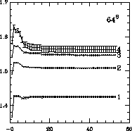
Figure 4.13:
Leading Even Eigenvalue on  Lattice
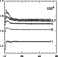
Figure 4.14:
Leading Even Eigenvalue on  Lattice
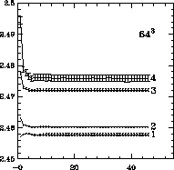
Figure 4.15:
Leading Odd Eigenvalue on  Lattice
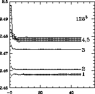
Figure 4.16:
Leading Odd Eigenvalue on  Lattice
Finally, perhaps the most important number, because it can be
determined the most accurately, is  . By comparing the fifth
blocking
level on the
. By comparing the fifth
blocking
level on the  lattice to the fourth on
the
lattice to the fourth on
the  lattice for both coupling values and taking a weighted mean,
we obtain
lattice for both coupling values and taking a weighted mean,
we obtain  , where again
the first error is statistical and the second is systematic.
, where again
the first error is statistical and the second is systematic.
Thus, MCRG calculations give us very accurate values for the three
critical parameters  ,
,  , and
, and  , and give a
reasonable estimate for
, and give a
reasonable estimate for  . Each parameter is obtained
independently and directly from the data. We have shown that
truncation and finite-size errors at all but the highest
blocking
level have been reduced to below the
statistical errors. Future high statistics simulations on
. Each parameter is obtained
independently and directly from the data. We have shown that
truncation and finite-size errors at all but the highest
blocking
level have been reduced to below the
statistical errors. Future high statistics simulations on  lattices will significantly reduce the remaining errors and allow us to
determine the exponents very accurately.
lattices will significantly reduce the remaining errors and allow us to
determine the exponents very accurately.
Next:
4.4.3 Potts Model
Up:
4.4 Spin Models
Previous:
4.4.1 Introduction
Guy Robinson
Wed Mar 1 10:19:35 EST 1995
4.4.3 Potts Model
Next:
4.4.4 XY Model
Up:
4.4 Spin Models
Previous:
4.4.2 Ising Model
The
q
-state Potts model
[
Potts:52a
] consists of a
lattice of spins  , which can take
q
different values, and whose
Hamiltonian is
, which can take
q
different values, and whose
Hamiltonian is

For
q=2
, this is equivalent to the Ising model. The Potts model is thus a
simple extension of the Ising model; however, it has a much richer phase
structure, which makes it an important testing ground for new theories and
algorithms in the study of critical phenomena [
Wu:82a
].
Monte Carlo
simulations of Potts models have
traditionally used local algorithms such as that of
Metropolis,
et al. [
Metropolis:53a
], however,
these algorithms have the major drawback that near a phase transition,
the autocorrelation time (the number of sweeps needed to generate a
statistically independent configuration) increases approximately as
 , where
L
is the linear size of the lattice. New algorithms
have recently been developed that dramatically reduce this ``critical
slowing down''
by updating clusters of
spins at a time (these algorithms are described in
Section
12.6
). The original cluster algorithm of Swendsen and
Wang (SW) was implemented for the Potts model [
Swendsen:87a
], and
there is a lot of interest in how well cluster algorithms perform for
this model. At present, there are very few theoretical results known
about cluster algorithms,
and theoretical
advances are most likely to come from first studying the simplest
possible models.
, where
L
is the linear size of the lattice. New algorithms
have recently been developed that dramatically reduce this ``critical
slowing down''
by updating clusters of
spins at a time (these algorithms are described in
Section
12.6
). The original cluster algorithm of Swendsen and
Wang (SW) was implemented for the Potts model [
Swendsen:87a
], and
there is a lot of interest in how well cluster algorithms perform for
this model. At present, there are very few theoretical results known
about cluster algorithms,
and theoretical
advances are most likely to come from first studying the simplest
possible models.
We have made a high statistics study of the SW algorithm and the single
cluster Wolff algorithm [
Wolff:89b
], as well as a number of variants of
these algorithms, for the
q=2
and
q=3
Potts models in two dimensions
[
Baillie:90n
]. We measured the autocorrelation time  in the
energy (a local operator) and the magnetization (a global one) on lattice
sizes from
in the
energy (a local operator) and the magnetization (a global one) on lattice
sizes from  to
to  . About 10 million sweeps were required for each
lattice size in order to measure autocorrelation times to within about 1 percent.
From these values, we can extract the dynamic critical exponent
z
, given
by
. About 10 million sweeps were required for each
lattice size in order to measure autocorrelation times to within about 1 percent.
From these values, we can extract the dynamic critical exponent
z
, given
by  , where
  is measured at the infinite volume
critical point (which is known exactly for the two-dimensional Potts model).
is measured at the infinite volume
critical point (which is known exactly for the two-dimensional Potts model).
The simulations were performed on a number of different parallel
computers. For lattice sizes of  or less, it is possible to run
independent simulations on each processor of a parallel machine,
enabling us to obtain 100 percent efficiency by running 10 or 20 runs
for each lattice size in parallel, using different random
number
streams. These calculations were done
using a 32-processor Meiko
Computing Surface, a
20-processor Sequent
Symmetry, a 20-processor
Encore
Multimax, and a 96-processor BBN GP1000
Butterfly
, as well as a network of SUN
workstations. The calculations ook approximately 15,000
processor-hours. For the largest lattice sizes,
or less, it is possible to run
independent simulations on each processor of a parallel machine,
enabling us to obtain 100 percent efficiency by running 10 or 20 runs
for each lattice size in parallel, using different random
number
streams. These calculations were done
using a 32-processor Meiko
Computing Surface, a
20-processor Sequent
Symmetry, a 20-processor
Encore
Multimax, and a 96-processor BBN GP1000
Butterfly
, as well as a network of SUN
workstations. The calculations ook approximately 15,000
processor-hours. For the largest lattice sizes,  and
and  , a
parallel cluster algorithm was required, due to the large amount of
calculation (and memory) required. We have used the
self-labelling
algorithm described in
Section
12.6
, which gives fairly good efficiencies of about
70 percent on the machines we have used (an nCUBE-1 and a Symult
S2010), by doing multiple runs of 32 nodes each for the
, a
parallel cluster algorithm was required, due to the large amount of
calculation (and memory) required. We have used the
self-labelling
algorithm described in
Section
12.6
, which gives fairly good efficiencies of about
70 percent on the machines we have used (an nCUBE-1 and a Symult
S2010), by doing multiple runs of 32 nodes each for the  lattice, and 64 nodes for
  . Since this problem does not
vectorize, using all 512 nodes of the nCUBE gives a performance
approximately five times that of a single processor
CRAY X-MP,
while all 192 nodes of the Symult is equivalent
to about six CRAYs. The calculations on these machines have so far
taken about 1000 hours.
. Since this problem does not
vectorize, using all 512 nodes of the nCUBE gives a performance
approximately five times that of a single processor
CRAY X-MP,
while all 192 nodes of the Symult is equivalent
to about six CRAYs. The calculations on these machines have so far
taken about 1000 hours.
Results for the autocorrelation times of the energy for the Wolff and SW
algorithms are shown in Figure
4.17
for
q=2
and
Figure
4.18
for
q=3
. As can be seen, the Wolff algorithm has
smaller autocorrelation times than SW. However, the dynamical critical
exponents for the two algorithms appear to be identical, being approximately
 and
and  for
q=2
and
q=3
respectively (shown as
straight lines in Figures
4.17
and
4.18
),
compared to values of approximately 2 for the standard Metropolis
algorithm.
for
q=2
and
q=3
respectively (shown as
straight lines in Figures
4.17
and
4.18
),
compared to values of approximately 2 for the standard Metropolis
algorithm.
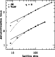
Figure 4.17:
Energy Autocorrelation Times,
q=2
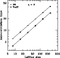
Figure 4.18:
Energy Autocorrelation Times,
q=3
Burkitt and Heermann [
Heermann:90a
] have suggested that the increase in
the autocorrelation time is a logarithmic one, rather than a power law for
the
q=2
case (the Ising model), that is,
z = 0
. Fits to this
are shown as dotted lines in Figure
4.17
. These have
smaller  values than the power law fits, favoring logarithmic
behavior. However, it is very difficult to distinguish between a logarithm
and a small power even on lattices as large as
values than the power law fits, favoring logarithmic
behavior. However, it is very difficult to distinguish between a logarithm
and a small power even on lattices as large as  . In any case, the
performance of the cluster algorithms for the Potts model is quite
extraordinary, with autocorrelation times for the
. In any case, the
performance of the cluster algorithms for the Potts model is quite
extraordinary, with autocorrelation times for the  lattice
hundreds of times smaller than for the Metropolis algorithm. In the future,
we hope to use the cluster algorithms to perform greatly improved Monte Carlo
simulations of various Potts models, to study their critical behavior.
lattice
hundreds of times smaller than for the Metropolis algorithm. In the future,
we hope to use the cluster algorithms to perform greatly improved Monte Carlo
simulations of various Potts models, to study their critical behavior.
There is little theoretical understanding of why cluster algorithms
work so well, and in particular there is no theory which predicts the
dynamic critical exponents for a given model. These values can
currently only be obtained from measurements using Monte Carlo
simulation. Our results, which are the best currently available, are
shown in Table
4.6
. We would like to know why, for example,
critical slowing down is virtually eliminated for the two-dimensional
2-state Potts model, but
z
is nearly one for the 4-state model; and why
the dynamic critical exponents for the SW and Wolff algorithms are
approximately the same in two dimensions, but very different in higher
dimensions.
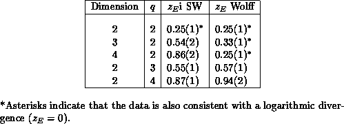
Table 4.6:
Measured Dynamic Critical Exponents for Potts Model Cluster Algorithms.
The only rigorous analytic result so far obtained for cluster
algorithms was derived by Li and Sokal [
Li:89a
]. They showed that
the autocorrelation time for the energy using the SW algorithm is
bounded (as a function of the lattice size) by the specific heat  ,
that is,
,
that is,  , which implies
that the corresponding dynamic critical exponent is bounded by
, which implies
that the corresponding dynamic critical exponent is bounded by
 , where
  and
and  are critical exponents
measuring the divergence at the critical point of the specific heat and
the correlation length, respectively. A similar bound has also been
derived for the Metropolis algorithm, but with the susceptibility
exponent substituted for the specific heat exponent.
are critical exponents
measuring the divergence at the critical point of the specific heat and
the correlation length, respectively. A similar bound has also been
derived for the Metropolis algorithm, but with the susceptibility
exponent substituted for the specific heat exponent.
No such result is known for the Wolff algorithm, so we have attempted
to check this result empirically using simulation
[
Coddington:92a
]. We found that for the Ising model in two, three,
and four dimensions, the above bound appears to be satisfied (at least
to a very good approximation); that is, there are constants
a
and
b
such that  , and thus
 , for the Wolff algorithm.
This led us to investigate similar empirical relations between dynamic
and static quantities for the SW algorithm. The power of cluster
update algorithms comes from the fact that they flip large clusters of
spins at a time. The average size of the largest SW cluster (scaled by
the lattice volume),
m
, is an estimator of the magnetization for the
Potts model, and the exponent  characterizing the
divergence of the magnetization has values which are similar to our
measured values for the dynamic exponents of the SW algorithm. We
therefore scaled the SW autocorrelations by
m
, and found that within
the errors of the simulations, this gave either a constant (in three
and four dimensions) or a logarithm (in two dimensions). This implies
that the SW autocorrelations scale in the same way (up to logarithmic
corrections) as the magnetization, that is,
characterizing the
divergence of the magnetization has values which are similar to our
measured values for the dynamic exponents of the SW algorithm. We
therefore scaled the SW autocorrelations by
m
, and found that within
the errors of the simulations, this gave either a constant (in three
and four dimensions) or a logarithm (in two dimensions). This implies
that the SW autocorrelations scale in the same way (up to logarithmic
corrections) as the magnetization, that is,  .
.
These simple empirical relations are very surprising, and if true,
would be the first analytic results equating dynamic quantities, which
are dependent on the Monte Carlo
algorithm used,
to static quantities, which depend only on the physical model. These
relations could perhaps stem from the fact that the dynamics of cluster
algorithms are closely linked to the physical properties of the system,
since the Swendsen-Wang clusters are just the Coniglio-Klein-Fisher
droplets which have been used to describe the critical behavior of
these systems [
Fisher:67a
] [
Coniglio:80a
].
We are currently doing further simulations to check whether these
relations hold up with larger lattices and better statistics, or
whether they are just good approximations. We are also trying to
determine whether similar results hold for the general
q
-state Potts
model. However, we have thus far only been able to find simple relations
for the
q=2
(Ising) model. This work is being done using both
parallel machines (the nCUBE-1, nCUBE-2, and Symult S2010) and networks
of DEC, IBM, and Hewlett-Packard workstations. These high-performance
RISC workstations were especially useful in obtaining good results for
the Wolff algorithm, which does not vectorize or parallelize, apart
from the trivial parallelism we used in running independent simulations
on different processors.
Next:
4.4.4 XY Model
Up:
4.4 Spin Models
Previous:
4.4.2 Ising Model
Guy Robinson
Wed Mar 1 10:19:35 EST 1995
4.4.4 XY Model
Next:
4.4.5 O(3) Model
Up:
4.4 Spin Models
Previous:
4.4.3 Potts Model
The XY (or O(2)) model
consists of a set of continuous
valued spins regularly arranged on a two-dimensional square lattice.
Fifteen years ago, Kosterlitz and Thouless
(KT) predicted that this system would undergo a phase
transition
as one changed from a low-temperature
spin wave phase to a high-temperature phase with unbound vortices. KT
predicted an approximate transition temperature,  , and the
following unusual exponential singularity in the correlation length and
magnetic susceptibility:
, and the
following unusual exponential singularity in the correlation length and
magnetic susceptibility:

with

where  and the correlation function exponent
  is defined
by the relation
is defined
by the relation  .
.
Our simulation [
Gupta:88a
] was done on the 128-node FPS
(Floating Point Systems) T-Series hypercube at Los Alamos. FPS
software allowed the use of C with a software model similar
(communication implemented by subroutine call) to that used on the
hypercubes at Caltech. Each FPS node is built around Weitek
floating-point units, and we achieved  per node in this
application. The total machine ran at
per node in this
application. The total machine ran at  , or at about
twice the performance of one processor of a CRAY X-MP
for
this application. We use a
1-D
torus topology for communications,
with each node processing a fraction of the rows. Each row is divided
into red/black alternating sites of spins and the vector loop is over a
given color. This gives a natural data structure of (
, or at about
twice the performance of one processor of a CRAY X-MP
for
this application. We use a
1-D
torus topology for communications,
with each node processing a fraction of the rows. Each row is divided
into red/black alternating sites of spins and the vector loop is over a
given color. This gives a natural data structure of ( )
words for lattices of size
)
words for lattices of size  . The internode
communications, in both lattice update and measurement of observables,
can be done asynchronously and are a negligible overhead.
. The internode
communications, in both lattice update and measurement of observables,
can be done asynchronously and are a negligible overhead.
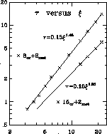
Figure 4.19:
Autocorrelation Times for the XY Model
Previous numerical work was unable to confirm the KT theory, due to limited
statistics and small lattices. Our high-statistics simulations are done on
 ,
,  ,
,  , and
, and  lattices using a combination of
over-relaxed and Metropolis
algorithms which
decorrelates as
lattices using a combination of
over-relaxed and Metropolis
algorithms which
decorrelates as  . (For comparison, a
Metropolis algorithm decorrelates as
. (For comparison, a
Metropolis algorithm decorrelates as  .) Each
configuration represents
.) Each
configuration represents  over-relaxed sweeps through the
lattice followed by
over-relaxed sweeps through the
lattice followed by  Metropolis sweeps. Measurement of
observables is made on every configuration. The over-relaxed algorithm
consists of reflecting the spin at a given site about
Metropolis sweeps. Measurement of
observables is made on every configuration. The over-relaxed algorithm
consists of reflecting the spin at a given site about  , where
 is the sum of the nearest-neighbor spins, that is,

This implementation [
Creutz:87a
], [
Brown:87a
] of the
over-relaxed algorithm is microcanonical, and it reduces critical
slowing down even though it is a local algorithm. The ``hit'' elements
for the Metropolis algorithm are generated as  , where
 is a uniform random number
in the
interval
is a uniform random number
in the
interval  , and
, and  is adjusted to
give an acceptance rate of 50 to 60 percent. The Metropolis hits make
the algorithm ergodic, but their effectiveness is limited to local
changes in the energy. In Figure
4.19
, we show the
autocorrelation time
is adjusted to
give an acceptance rate of 50 to 60 percent. The Metropolis hits make
the algorithm ergodic, but their effectiveness is limited to local
changes in the energy. In Figure
4.19
, we show the
autocorrelation time  vs. the correlation length
  ; for
; for
 ,
,  we extract
  , and
for
, and
for  ,
,  we get
  .
.
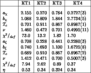
Table 4.7:
Results of the XY Model Fits: (a)  in T, and (b)
  in T Assuming the KT Form. The fits KT1-3 are pseudominima while KT4 is
the true minimum. All data points are included in the fits and we give the
in T Assuming the KT Form. The fits KT1-3 are pseudominima while KT4 is
the true minimum. All data points are included in the fits and we give the
 for each fit and an estimate of the exponent
  .
.
We ran at 14 temperatures near the phase transition
and made unconstrained fits to all 14 data points (four
parameter fits according to Equation
4.24
), for both the
correlation length (Figure
4.20
) and susceptibility
(Figure
4.21
). The key to the interpretation of the data
is the fits. We find that fitting programs (e.g., MINUIT, SLAC) move
incredibly slowly towards the true minimum from certain points (which
we label spurious minima), which, unfortunately, are the attractors for
most starting points. We found three such spurious minima (KT1-3) and
the true minimum KT4, as listed in Table
4.7
.
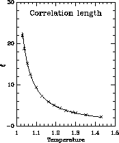
Figure 4.20:
Correlation Length for the XY Model
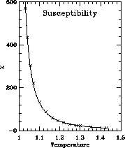
Figure 4.21:
Susceptibility for the XY Model
Thus, our data was found to be in excellent agreement with the KT theory and,
in fact, this study provides the first direct measurement of  from both
 and
and  data that is consistent with the KT predictions.
Next:
4.4.5 O(3) Model
Up:
4.4 Spin Models
Previous:
4.4.3 Potts Model
Guy Robinson
Wed Mar 1 10:19:35 EST 1995
4.4.5 O(3) Model
Next:
4.5 An Automata Model
Up:
4.4 Spin Models
Previous:
4.4.4 XY Model
The XY model is the simplest O(N) model, having
N=2
, the O(N) model
being a set of rotors (N-component continuous valued spins) on an
N-sphere. For  , this model is asymptotically free
[
Polyakov:75a
], and for
N=3
, there exist so called instanton
solutions. Some of these properties are analogous to those of gauge
theories in four dimensions; hence, these models are interesting. In
particular, the O(3) model
in two dimensions should
shed some light on the asymptotic freedom of QCD (SU(3)) in four
dimensions. The predictions of the renormalization group for the
susceptibility
, this model is asymptotically free
[
Polyakov:75a
], and for
N=3
, there exist so called instanton
solutions. Some of these properties are analogous to those of gauge
theories in four dimensions; hence, these models are interesting. In
particular, the O(3) model
in two dimensions should
shed some light on the asymptotic freedom of QCD (SU(3)) in four
dimensions. The predictions of the renormalization group for the
susceptibility  and inverse correlation length (i.e., mass gap)
m
in the O(3) model are [
Brezin:76a
]
and inverse correlation length (i.e., mass gap)
m
in the O(3) model are [
Brezin:76a
]

and

respectively. If
m
and  vary according to these equations,
without the correction of order
vary according to these equations,
without the correction of order  , they are said to follow
asymptotic scaling.
Previous work was able
to confirm that this picture is qualitatively correct, but was not able
to probe deep enough in the area of large correlation lengths to obtain
good agreement.
, they are said to follow
asymptotic scaling.
Previous work was able
to confirm that this picture is qualitatively correct, but was not able
to probe deep enough in the area of large correlation lengths to obtain
good agreement.
The combination of the over-relaxed algorithm and the computational
power of the FPS T-Series allowed us to simulate lattices of sizes up
to  . We were thus able to simulate at coupling constants that
correspond to correlation lengths up to 300, on lattices where
finite-size effects are negligible. We were also able to gather large
statistics and thus obtain small statistical errors. Our simulation is
in good agreement with similar cluster calculations
[Wolff:89b;90a]. Thus, we have validated and
extended these results in a regime where our algorithm is the only
known alternative to clustering.
. We were thus able to simulate at coupling constants that
correspond to correlation lengths up to 300, on lattices where
finite-size effects are negligible. We were also able to gather large
statistics and thus obtain small statistical errors. Our simulation is
in good agreement with similar cluster calculations
[Wolff:89b;90a]. Thus, we have validated and
extended these results in a regime where our algorithm is the only
known alternative to clustering.
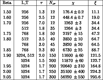
Table 4.8:
Coupling Constant, Lattice Size, Autocorrelation Time, Number of
Overrelaxed Sweeps, Susceptibility, and Correlation Length for the O(3)
Model
We have made extensive runs at 10 values of the coupling constant. At the
lowest  , several hundred thousand sweeps were collected, while for the
largest values of
, several hundred thousand sweeps were collected, while for the
largest values of  , between
50,000
and
100,000
sweeps were made.
Each sweep consists of between 10 iterations through the lattice at the
former end and 150 iterations at the latter. The statistics we have gathered
are equivalent to about 200 days, use of the full 128-node FPS machine.
, between
50,000
and
100,000
sweeps were made.
Each sweep consists of between 10 iterations through the lattice at the
former end and 150 iterations at the latter. The statistics we have gathered
are equivalent to about 200 days, use of the full 128-node FPS machine.
Our results for the correlation length and susceptibility for each
coupling  and lattice size are shown in Table
4.8
.
The autocorrelation times are also shown. The quantities measured on
different-sized lattices at the same
and lattice size are shown in Table
4.8
.
The autocorrelation times are also shown. The quantities measured on
different-sized lattices at the same  agree, showing that the
infinite volume limit has been reached.
agree, showing that the
infinite volume limit has been reached.
To compare the behavior of the correlation length and susceptibility
with the asymptotic scaling predictions, we use the ``correlation
length defect''  and ``susceptibility defect''
 , which are defined as follows:
  ,
,  ,
so that asymptotic scaling is seen if
,
so that asymptotic scaling is seen if  ,
,  go to constants as
  . These defects are shown
in Figures
4.22
and
4.23
, respectively. It
is clear that asymptotic scaling does not set in for
. These defects are shown
in Figures
4.22
and
4.23
, respectively. It
is clear that asymptotic scaling does not set in for  , but
it is not possible to draw a clear conclusion for
, but
it is not possible to draw a clear conclusion for  -though
the trends of the last two or three points may be toward constant behavior.
-though
the trends of the last two or three points may be toward constant behavior.
Figure 4.22:
Correlation Length Defect Versus the Coupling Constant for the O(3)
Model
Figure 4.23:
Susceptibility Defect Versus the Coupling Constant for the O(3) Model
Figure 4.24:
Decorrelation Time  Versus Number of Over-relations Sweeps
 for Different Values of
We gauged the speed of the algorithm in producing statistically independent
configurations by measuring the autocorrelation time  . We used this to
estimate the dynamical critical exponent
z
, which is defined by
. We used this to
estimate the dynamical critical exponent
z
, which is defined by  . For constant
  , our fits give
  . However,
we discovered that by increasing
. However,
we discovered that by increasing  in rough proportion to
  , we
can improve the performance of the algorithm significantly. To compare the
speed of decorrelation between runs with different
, we
can improve the performance of the algorithm significantly. To compare the
speed of decorrelation between runs with different  , we define a new
quantity, which we call ``effort,''
, we define a new
quantity, which we call ``effort,''  . This measures
the computational effort expended to obtain a decorrelated configuration. We
define a new exponent
. This measures
the computational effort expended to obtain a decorrelated configuration. We
define a new exponent  from
from  , where
  is chosen to keep
  constant. We also found that the behavior of
the decorrelation time can be approximated over a good range by
constant. We also found that the behavior of
the decorrelation time can be approximated over a good range by

A fit to the set of points ( ,
,  ,
,  ) gives
 ,
,  . Thus,
  is
significantly lower than
z
. Figure
4.24
shows
is
significantly lower than
z
. Figure
4.24
shows  versus
 , with the fits shown as solid lines.
Next:
4.5 An Automata Model
Up:
4.4 Spin Models
Previous:
4.4.4 XY Model
Guy Robinson
Wed Mar 1 10:19:35 EST 1995
4.5 An Automata Model of Granular Materials
Next:
4.5.1 Introduction
Up:
4 Synchronous Applications I
Previous:
4.4.5 O(3) Model
Other References
HPFA Applications
Guy Robinson
Wed Mar 1 10:19:35 EST 1995
4.5.1 Introduction
Next:
4.5.2 Comparison to Particle
Up:
4.5 An Automata Model
Previous:
4.5 An Automata Model
Physical systems comprised of discrete, macroscopic particles or
grains which are not bonded to one another are important in civil,
chemical, and agricultural engineering, as well as in natural
geological and planetary environments. Granular systems
are observed in rock slides, sand
dunes, clastic
sediments, snow avalanches, and planetary rings. In engineering and
industry they are found in connection with the processing of cereal
grains, coal, gravel, oil shale, and powders, and are well known to
pose important problems associated with the movement of sediments by
streams, rivers, waves, and the wind.
The standard approach to the theoretical modelling of multiparticle systems
in physics has been to treat the system as a continuum and to formulate the
model in terms of differential equations. As an example, the science of soil
mechanics has traditionally focussed mainly on quasi-static granular systems,
a prime objective being to define and predict the conditions under which
failure of the granular soil system will occur. Soil mechanics is a
macroscopic continuum model requiring an explicit constitutive law relating,
for example, stress and strain. While very successful for the low-strain
quasi-static applications for which it is intended, it is not clear how it
can be generalized to deal with the high-strain, explicitly time-dependent
phenomena which characterize a great many other granular systems of interest.
Attempts at obtaining a generalized theory of granular systems using a
differential equation formalism [
Johnson:87a
] have met with limited
success.
An alternate approach to formulating physical theories can be found in
the concept of cellular automata
, which was first
proposed by Von Neumann in 1948. In this approach, the space of a physical
problem would be divided up into many small, identical cells each of which
would be in one of a finite number of states. The state of a cell would
evolve according to a rule that is both local (involves only the cell itself
and nearby cells) and universal (all cells are updated simultaneously using
the same rule).
The Lattice Grain Model
[
Gutt:89a
]
(LGrM) we discuss here is a microscopic, explicitly time-dependent,
cellular automata
model, and can be applied
naturally to high-strain events. LGrM carries some attributes of both
particle dynamics
models [
Cundall:79a
],
[Haff:87a;87b], [
Walton:84a
],
[
Werner:87a
] (PDM), which are based explicitly on Newton's second
law, and lattice gas models [
Frisch:86a
], [
Margolis:86a
]
(LGM), in that its fundamental element is a discrete particle, but
differs from these substantially in detail. Here we describe the
essential features of LGrM, compare the model with both PDM and LGM,
and finally discuss some applications.
Next:
4.5.2 Comparison to Particle
Up:
4.5 An Automata Model
Previous:
4.5 An Automata Model
Guy Robinson
Wed Mar 1 10:19:35 EST 1995
4.5.2 Comparison to Particle Dynamics Models
Next:
4.5.3 Comparison to Lattice
Up:
4.5 An Automata Model
Previous:
4.5.1 Introduction
The purpose of the lattice grain model is to predict the behavior of
large numbers of grains (10,000 to 1,000,000) on scales much larger
than a grain diameter. In this respect, it goes beyond the particle
dynamics calculations of Section
9.2
, which are limited to no
more than  grains by currently available computing
resources [
Cundall:79a
], [Haff:87a;87b],
[
Walton:84a
], [
Werner:87a
]. The particle
dynamics models follow the motion of each individual grain exactly, and
may be formulated in one of two ways depending upon the model adopted
for particle-particle interactions.
grains by currently available computing
resources [
Cundall:79a
], [Haff:87a;87b],
[
Walton:84a
], [
Werner:87a
]. The particle
dynamics models follow the motion of each individual grain exactly, and
may be formulated in one of two ways depending upon the model adopted
for particle-particle interactions.
In one formulation, the interparticle contact times are assumed to be of
finite duration, and each particle may be in simultaneous contact with
several others [
Cundall:79a
], [
Haff:87a
], [
Walton:84a
],
[
Werner:87a
]. Each particle obeys Newton's law,
F = ma
, and a
detailed integration of the equations of motion of each particle is performed.
In this form, while useful for applications involving a much smaller number
of particles than LGrM allows, PDM cannot compete with LGrM for systems
involving large numbers of grains because of the complexity of PDM
``automata.''
In the second, simpler formulation, the interparticle contact times are
assumed to be of infinitesimal duration, and particles undergo only binary
collisions (the hard-sphere collisional models) [
Haff:87b
]. Hard-sphere
models usually rely upon a collision-list ordering of collision events to
avoid the necessity of checking all pairs of particles for overlaps at each
time step. In regions of high particle number density, collisions are very
frequent; and thus in problems where such high-density zones appear,
hard-sphere models spend most of their time moving particles through very
small distances using very small time steps. In granular flow, zones of
stagnation where particles are very nearly in contact much of the time, are
common, and the hard-sphere model is therefore unsuitable, at least in its
simplest form, as a model of these systems. LGrM avoids these difficulties
because its time-stepping is controlled, not by a collision list but by a scan
frequency, which in turn is a function of the speed of the fastest particle
and is independent of number density. Furthermore, although fundamentally a
collisional model, LGrM can also mimic the behavior of consolidated or
stagnated zones of granular material in a manner which will be described.
Next:
4.5.3 Comparison to Lattice
Up:
4.5 An Automata Model
Previous:
4.5.1 Introduction
Guy Robinson
Wed Mar 1 10:19:35 EST 1995
4.5.3 Comparison to Lattice Gas Models
Next:
4.5.4 The Rules for
Up:
4.5 An Automata Model
Previous:
4.5.2 Comparison to Particle
LGrM closely resembles LGM [
Frisch:86a
], [
Margolis:86a
] in some
respects. First, for two-dimensional applications, the region of space in
which the particles are to move is discretized into a triangular
lattice-work, upon each node of which can reside a particle. The particles
are capable of moving to neighboring cells at each tick of the clock, subject
to certain simple rules. Finally, two particles arriving at the same cell
(LGM) or adjacent cells (LGrM) at the same time, may undergo a ``collision''
in which their outgoing velocities are determined according to specified
rules chosen to conserve momentum.
Each of the particles in LGM has the same magnitude of velocity and is
allowed to move in one of six directions along the lattice, so that
each particle travels exactly one lattice spacing in each time step.
The single-velocity magnitude means that all collisions between
particles are perfectly elastic and that energy conservation is
maintained simply through particle number conservation. It also means
that the temperature of the gas is uniform throughout time and space,
thus limiting the application of LGM to problems of low Mach number.
An exclusion principle is maintained in which no two particles of the
same velocity may occupy one lattice point. Thus, each lattice point
may have no more than six particles, and the state of a lattice point
can be recorded using only six bits.
LGrM differs from LGM in that it has many possible velocity states, not
just six. In particular, in LGrM not only the direction but the
magnitude of the velocity can change in each collision. This is a
necessary condition because the collision of two macroscopic particles
is always inelastic, so that mechanical energy is not conserved. The
LGrM particles satisfy a somewhat different exclusion principle: No
more than one particle at a time may occupy a single site. This
exclusion principle allows LGrM to capture some of the volume-filling
properties of granular material-in particular, to be able to
approximate the behavior of static granular masses.
The determination of the time step is more critical in LGrM than in LGM.
If the time step is long enough that some particles travel several lattice
spacings in one clock tick, the problem of finding the intersection of
particle trajectories arises. This involves much computation and
defeats the purpose of an automata approach. A very short time step would
imply that most particles would not move even a single lattice spacing.
Here we choose a time step such that the fastest particle will move
exactly one lattice spacing. A ``position offset'' is stored for each of the
slower particles, which are moved accordingly when the offset exceeds
one-half lattice spacing. These extra requirements for LGrM automata imply a
slower computation speed than expected in LGM simulations; but, as a
dividend, we can compute inelastic grain flows of potential engineering and
geophysical interest.
Next:
4.5.4 The Rules for
Up:
4.5 An Automata Model
Previous:
4.5.2 Comparison to Particle
Guy Robinson
Wed Mar 1 10:19:35 EST 1995
4.5.4 The Rules for the Lattice Grain Model
Next:
4.5.5 Implementation on a
Up:
4.5 An Automata Model
Previous:
4.5.3 Comparison to Lattice
In order to keep the particle-particle interaction rules as simple as
possible, all interparticle contacts, whether enduring contacts or true
collisions, will be modelled as collisions. Collisions that model
enduring contacts will transmit, in each time step, an impulse equal to
the force of the enduring contact multiplied by the time step. The
fact that collisions take place between particles on adjacent lattice
nodes means that some particles may undergo up to six collisions in a
time step. For simplicity, these collisions will be resolved as a
series of binary collisions. The order in which these collisions are
calculated at each lattice node, as well as the order in which the
lattice nodes are scanned, is now an important consideration.
The rules of the Lattice Grain Model may be summarized as follows:
-
The particles reside on the nodes of a two-dimensional triangular
lattice, obeying the exclusion principle that no node may have more than one
particle.
-
Each particle has two components of velocity, which may take on any
value. At the beginning of each time step, each particle's velocity is
incremented due to the acceleration of gravity.
-
The size of each time step is set so that the fastest particle will
travel one lattice spacing in that time step.
-
Two components of a ``position offset'' are maintained for each
particle. This offset is incremented after the velocities in each time step
according to gravitational acceleration and the particle's velocity:

where:
Once the offset exceeds half the distance to the nearest lattice node, and
that node is empty, the particle is moved to that node, and its offset is
decremented appropriately. Also, in a collision, the component of the offset
along the line connecting the centers of the colliding particles is set to
zero.
-
The order in which the lattice is scanned is chosen so as not to create
a coupling between the scan pattern and the particle motions. Thus, the
particle position updates are done on every third lattice point of every
third row, with this pattern being repeated nine times to cover all
lattice sites.
-
Particle collisions are calculated assuming that they are smooth hard
disks with a given coefficient of restitution. Particles on adjacent nodes
are assumed to collide if their relative velocity is bringing them together.
The following order has been adopted for evaluating possible collisions on
odd time steps: 3b, 3c, 3f, 2f, 2c, 2b, 4b, 4c, 4f, 1f, 1c, 1b; and for even
time steps: 1b, 1c, 1f, 4f, 4c, 4b, 2b, 2c, 2f, 3f, 3c, 3b (where the lattice
numbers and collision directions are defined in Figure
4.25
).
-
In order to incorporate a container, wall, or other barrier within
these rules, a second type of particle is introduced-the wall particle.
This particle is similar to the movable particles, and interacts with them
through binary collisions (with a separately defined inelasticity), but is
regarded as having infinite mass. To allow for the introduction of shearing
motion from a wall (as in a Couette flow problem), the particles making up the
wall are given a common constant velocity, which is used in the usual fashion
for calculating the results of collisions. However, the position of the wall
particles in the lattice remains fixed throughout the simulation.
-
Though a single particle does not accurately predict the trajectory of
a single grain, we still regard each particle as representing one grain when
we are extracting information from the simulation regarding the behavior of
groups of grains. Thus, the size of one particle, as well as the spacing
between lattice points, is taken to be one grain-diameter.
The transmission of ``static'' contact forces within a mass of grains (as in
grains at rest in a gravitational field) is handled naturally within the
above framework. Though a particle in a static mass of grains may be
nominally at rest, its velocity may be nonzero (due to gravitational or
pressure forces); and it will transmit the appropriate force (in the form of
an impulse) to the particles under it by means of collisions. When these
impulses are averaged over several time steps, the proper weights and
pressures will emerge.
Figure 4.25:
Definition of Lattice Numbers and Collision Directions
Next:
4.5.5 Implementation on a
Up:
4.5 An Automata Model
Previous:
4.5.3 Comparison to Lattice
Guy Robinson
Wed Mar 1 10:19:35 EST 1995
4.5.5 Implementation on a Parallel Computer
Next:
4.5.6 Simulations
Up:
4.5 An Automata Model
Previous:
4.5.4 The Rules for
When implementing this algorithm on a computer, what is stored in the
computer's memory is information concerning each point in the lattice,
regardless of whether or not there is a particle at that lattice point.
This allows for very efficient checking of the space around each
particle for the presence of other particles (i.e., information
concerning the six adjacent points in a triangular lattice will be found at
certain known locations in memory). The need to keep information on empty
lattice points in memory does not entail as great a penalty as might be
thought; many lattice grain model problems involve a high density of
particles, typically one for every one to four lattice points, and the memory
cost per lattice point is not large. The memory requirements for the
implementation of LGrM as described here are five variables per lattice
site: two components of position, two of velocity, and one
status variable, which denotes an empty site, an occupied site, or a bounding
``wall'' particle. If each variable is stored using four bytes of memory,
then each lattice point requires 20 bytes.
The standard configuration for a simulation consists of a lattice with a
specified number of rows and columns bounded at the top and bottom by two
rows of wall particles (thus forming the top and bottom walls of the problem
space), and with left and right edges connected together to form periodic
boundary conditions. Thus, the boundaries of the lattice are handled
naturally within the normal position updating and collision rules, with very
little additional programming. (Note: Since the gravitational acceleration
can point in an arbitrary direction, the top and bottom walls can become side
walls for chute flow. Also, the periodic boundary conditions can be broken
by the placement of an additional wall, if so desired.)
Because of the nearest-neighbor type interactions involved in the model, the
computational scheme was well suited to an nCUBE parallel processor. For the
purpose of dividing up the problem, the hypercube architecture is unfolded
into a two-dimensional array, and each processor is given a roughly
equal-area section of the lattice. The only interaction between sections
will be along their common boundaries; thus, each processor will only need to
exchange information with its eight immediate neighbors. The program itself
was written in C under the Cubix/CrOS III operating system.
Next:
4.5.6 Simulations
Up:
4.5 An Automata Model
Previous:
4.5.4 The Rules for
Guy Robinson
Wed Mar 1 10:19:35 EST 1995
4.5.6 Simulations
Next:
4.5.7 Conclusion
Up:
4.5 An Automata Model
Previous:
4.5.5 Implementation on a
The LGrM simulations performed so far have involved from  to
to
 automata. Trial application runs included two-dimensional, vertical,
time-dependent flows in several geometries, of which two examples are given
here: Couette flow
and flow out of an hourglass-shaped
hopper.
automata. Trial application runs included two-dimensional, vertical,
time-dependent flows in several geometries, of which two examples are given
here: Couette flow
and flow out of an hourglass-shaped
hopper.
The standard Couette flow
configuration consists of
a fluid confined between two flat parallel plates of infinite extent,
without any gravitational accelerations. The plates move in opposite
directions with velocities that are equal and parallel to their
surfaces, which results in the establishment of a velocity gradient and
a shear stress in the fluid. For fluids that obey the
Navier-Stokes
equation, an analytical
solution is possible in which the velocity gradient and shear stress
are constant across the channel. If, however, we replace the fluid by
a system of inelastic grains, the velocity gradient will no longer
necessarily be constant across the channel. Typically, stagnation
zones or plugs form in the center of the channel with thin shear-bands
near the walls. Shear-band formation in flowing granular materials was
analyzed earlier by Haff and others [
Haff:83a
], [
Hui:84a
]
based on kinetic theory models.
The simulation was carried out with 5760 grains, located in a channel 60
lattice points wide by 192 long. Due to the periodic boundary conditions at
the left and right ends, the problem is effectively infinite in length. The
first simulation is intended to reproduce the standard Couette flow for a
fluid; consequently, the particle-particle collisions were given a coefficient
of restitution of 1.0 (i.e., perfectly elastic collisions) and the
particle-wall collisions were given a .75 coefficient of restitution. The
inelasticity of the particle-wall collisions is needed to simulate the
conduction of heat (which is being generated within the fluid) from the fluid
to the walls. The simulation was run until an equilibrium was established in
the channel (Figure
4.26
(a)). The average
x
- and
y
-components of velocity and the second moment of velocity, as functions of
distance across the channel, are plotted in Figure
4.26
(b).
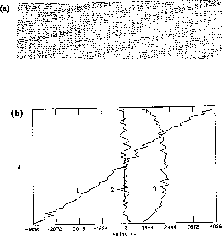
Figure 4.26:
(a) Elastic Particle Couette Flow; (b)
x
-component (1),
y
-component (2), and Second Moment (3) of Velocity
The second simulation used a coefficient of restitution of .75 for both the
particle-particle and particle-wall collisions. The equilibrium results are
shown in Figure
4.27
(a) and (b). As can
be seen from the plots, the flow consists of a central region of particles
compacted into a plug, with each particle having almost no velocity. Near
each of the moving walls, a region of much lower density has formed in which
most of the shearing motion occurs. Note the increase in value of the second
moment of velocity (the granular ``thermal velocity'') near the walls,
indicating that grains in this area are being ``heated'' by the high rate of
shear. It is interesting to note that these flows are turbulent in the sense
that shear stress is a quadratic, not a linear, function of shear rate.
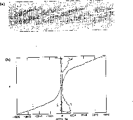
Figure 4.27:
(a) Inelastic Particle Couette Flow; (b)
x
-component (1),
y
-component (2), and Second Moment (3) of Velocity.
In the second problem, the flow of grains through a hopper or an hourglass
with an opening only a few grain diameters wide, was studied; the driving
force was gravity. This is an example of a granular system which contains a
wide range of densities, from groups of grains in static contact with one
another to groups of highly agitated grains undergoing true binary collisions.
Here, the number of particles used was 8310, and the lattice was 240 points
long by 122 wide. Additional walls were added to form the sloped sides of
the bin and to close off the bottom of the lattice to prevent the
periodic boundary conditions from reintroducing the falling particles back
into the bin (Figure
4.28
(a)). This is a typical feature of
automata modelling. It is often easier to configure the simulation to
resemble a real experiment-in this case by explicitly ``catching'' spent
grains-than by reprogramming the basic code to erase such particles.
The hourglass flow in Figure
4.28
(b) showed internal shear zones,
regions of stagnation, free-surface evolution toward an angle of repose, and
an exit flow rate approximately independent of pressure head, as observed
experimentally [
Tuzun:82a
]. It is hard to imagine that one could solve
a partial differential equation describing such a complex, multiple-domain,
time-dependent problem, even if the right equation were known (which is not
the case).
Figure 4.28:
(a) Initial Condition of Hourglass; (b) Hourglass Flow after 2048
Time Steps
Next:
4.5.7 Conclusion
Up:
4.5 An Automata Model
Previous:
4.5.5 Implementation on a
Guy Robinson
Wed Mar 1 10:19:35 EST 1995
4.5.7 Conclusion
Next:
Express and CrOS
Up:
4.5 An Automata Model
Previous:
4.5.6 Simulations
These exploratory numerical experiments show that an automata approach to
granular dynamics problems can be implemented on parallel computing machines.
Further work remains to be done to assess more quantitatively how well such
calculations reflect the real world, but the prospects are intriguing.
Guy Robinson
Wed Mar 1 10:19:35 EST 1995
Express and CrOS - Loosely Synchronous Message
Passing
Next:
5.1 Multicomputer Operating Systems
Up:
Parallel Computing Works
Previous:
4.5.7 Conclusion
Guy Robinson
Wed Mar 1 10:19:35 EST 1995
5.1 Multicomputer Operating Systems
Next:
5.2 A ``Packet''
History
Up:
Express and CrOS
Previous:
Express and CrOS
As already noted in Chapter
2
, the initial software used by
C P was called CrOS, although its modest functionality
hardly justified CrOS being called an operating system. Actually, this
is an interesting issue. In our original model, the ``real'' operating
system (UNIX
in our case) ran on the ``host'' that directly
or indirectly (via a network) connected to the hypercube. The nodes of
the parallel machine need only provide the minimal services necessary
to support user programs. This is the natural mode for all SIMD
systems and is still offered by several important MIMD multicomputers.
However, systems such as the IBM SP-1, Intel's Paragon series, and
Meiko's
CS-1 and 2 offer a full UNIX (or equivalent, such
as MACH) on each node. This has many advantages, including the ability
of the system to be arbitrarily configured-in particular we can
consider a multicomputer with
N
nodes as ``just''
N
``real''
computers connected by a high-performance network. This would lead to
particularly good performance on remote disk I/O,
such as
that needed for the Network File System (NFS). The design of an
operating system for the node is partly based on the programming usage
paradigm, and partly on the hardware. The original multicomputers all
had small node memories (
P was called CrOS, although its modest functionality
hardly justified CrOS being called an operating system. Actually, this
is an interesting issue. In our original model, the ``real'' operating
system (UNIX
in our case) ran on the ``host'' that directly
or indirectly (via a network) connected to the hypercube. The nodes of
the parallel machine need only provide the minimal services necessary
to support user programs. This is the natural mode for all SIMD
systems and is still offered by several important MIMD multicomputers.
However, systems such as the IBM SP-1, Intel's Paragon series, and
Meiko's
CS-1 and 2 offer a full UNIX (or equivalent, such
as MACH) on each node. This has many advantages, including the ability
of the system to be arbitrarily configured-in particular we can
consider a multicomputer with
N
nodes as ``just''
N
``real''
computers connected by a high-performance network. This would lead to
particularly good performance on remote disk I/O,
such as
that needed for the Network File System (NFS). The design of an
operating system for the node is partly based on the programming usage
paradigm, and partly on the hardware. The original multicomputers all
had small node memories ( on the Cosmic
Cube)
and could not possibly hold UNIX on a node.
Current multicomputers such as the CM-5, Paragon, and Meiko CS-2 would
consider
on the Cosmic
Cube)
and could not possibly hold UNIX on a node.
Current multicomputers such as the CM-5, Paragon, and Meiko CS-2 would
consider  a normal minimum node memory. This is easily
sufficient to hold a full UNIX implementation with the extra
functionality needed to support parallel programming. There are some,
such as IBM Owego (Execube), Seitz at Caltech (MOSAIC)
[Seitz:90a;92a], and Dally at MIT
(J Machine) [Dally:90a;92a], who
are developing very interesting families of highly parallel ``small
node'' multicomputers for which a full UNIX on each node may be
inappropriate.
a normal minimum node memory. This is easily
sufficient to hold a full UNIX implementation with the extra
functionality needed to support parallel programming. There are some,
such as IBM Owego (Execube), Seitz at Caltech (MOSAIC)
[Seitz:90a;92a], and Dally at MIT
(J Machine) [Dally:90a;92a], who
are developing very interesting families of highly parallel ``small
node'' multicomputers for which a full UNIX on each node may be
inappropriate.
Essentially, all the applications described in this book are not
sensitive to these issues, which would only affect the convenience of
program development and operating environment. C P's applications
were all developed using a simple message-passing system involving C
(and less often Fortran) node programs that sent messages to each
other via subroutine call. The key function of CrOS and Express,
described in Section
5.2
, was to provide this subroutine
library.
P's applications
were all developed using a simple message-passing system involving C
(and less often Fortran) node programs that sent messages to each
other via subroutine call. The key function of CrOS and Express,
described in Section
5.2
, was to provide this subroutine
library.
There are some important capabilities that a parallel computing
environment needs in addition to message passing and UNIX services.
These include:
-
scheduling of multiple users-at its simplest, this is
provided by space sharing with distinct sets of nodes assigned to
individual users. More sophisticated time sharing is also becoming
available.
-
performance visualization
or profiling-the C
 P tool is
described in Section
5.4
.
P tool is
described in Section
5.4
.
-
load balancing-this is still not well understood at
the operating system level, although at the data (user) level the
situation is much clearer. C
 P research is summarized in
Chapter
11
and Section
15.2
.
P research is summarized in
Chapter
11
and Section
15.2
.
-
parallel input/output-this topic needs a more elaborate discussion
given below.
We did not perform any major computations in C P that required
high-speed input/output capabilities. This reflects both our applications
mix and the poor I/O performance of the early hypercubes. The
applications described in Chapter
18
needed significant but
not high bandwidth
input/output during computation, as
did our analysis of radio astronomy data. However, the other
applications used input/output for checkpointing, interchange of
parameters between user and program, and in greatest volume, checkpoint
and restart. This input/output was typically performed between the
host and (node 0 of) the parallel ensemble. Section
5.2.7
and in
greater detail [
Fox:88a
] describe the Cubix
system,
which we developed to make this input/output more convenient. This
system was overwhelmingly preferred by the C
P that required
high-speed input/output capabilities. This reflects both our applications
mix and the poor I/O performance of the early hypercubes. The
applications described in Chapter
18
needed significant but
not high bandwidth
input/output during computation, as
did our analysis of radio astronomy data. However, the other
applications used input/output for checkpointing, interchange of
parameters between user and program, and in greatest volume, checkpoint
and restart. This input/output was typically performed between the
host and (node 0 of) the parallel ensemble. Section
5.2.7
and in
greater detail [
Fox:88a
] describe the Cubix
system,
which we developed to make this input/output more convenient. This
system was overwhelmingly preferred by the C P community as compared
to the conventional host-node programming style. Curiously, Cubix
seems to have made no impact on the ``real world.'' We are not aware
of any other group that has adopted it.
P community as compared
to the conventional host-node programming style. Curiously, Cubix
seems to have made no impact on the ``real world.'' We are not aware
of any other group that has adopted it.
Next:
5.2 A ``Packet''
History
Up:
Express and CrOS
Previous:
Express and CrOS
Guy Robinson
Wed Mar 1 10:19:35 EST 1995
5.2 A ``Packet''
History of Message-passingSystems
Next:
5.2.1 Prehistory
Up:
Express and CrOS
Previous:
5.1 Multicomputer Operating Systems
The evolution of the various message-passing paradigms used on the
Caltech/JPL machines involved three generations of hypercubes and many
different software concepts, which ultimately led to the development of
Express
,
a general, asynchronous buffered
communication system for heterogeneous multiprocessors.
Originally designed, developed, and used by scientists with
applications-oriented research goals, the Caltech/JPL system software
was written to generate near-term needed capability. Neither hindered
nor helped by any preconceptions about the type of software that should
be used for parallel processing, we simply built useful software and
added it to the system library.
Hence, the software evolved from primitive hardware-dependent
implementations into a sophisticated runtime library, which embodied
the concepts of ``loose synchronization,''
domain decomposition, and machine independence. By the time the
commercial machines started to replace our homemade hypercubes, we had
evolved a programming model that allowed us to develop and debug code
effectively, port it between different parallel computers, and run with
minimal overheads. This system has stood the test of time and,
although there are many other implementations, the functionality of
CrOS and Express appears essentially correct. Many of the ideas
described in this chapter, and the later
Zipcode
System of Section
16.1
, are embodied in the current
message-passing standards activity, MPI
[
Walker:94a
].
A detailed description of CrOS and Express will be found in
[
Fox:88a
] and [
Angus:90a
], and is not repeated here.
How did this happen?
Guy Robinson
Wed Mar 1 10:19:35 EST 1995
5.2.1 Prehistory
Next:
5.2.2 Application-driven Development
Up:
5.2 A ``Packet''
History
Previous:
5.2 A ``Packet''
History
The original hypercubes described in Chapter
20
, the Cosmic
Cube
[
Seitz:85a
], and Mark II
[
Tuazon:85a
] machines, had been designed and built as exploratory
devices. We expected to be able to do useful physics and, in particular, were
interested in high-energy physics. At that time, we were merely trying to
extract exciting physics from an untried technology. These first machines
came equipped with ``64-bit FIFOs,'' meaning that at a software level, two
basic communication routines were available:
rdELT(packet, chan)
wtELT(packet, chan).
The latter pushed a 64-bit ``packet'' into the indicated hypercube
channel,
which was then extracted with the
rdELT
function. If the read happened before the write, the
program in the reading node stopped and waited for the data to show up.
If the writing node sent its data before the reading node was ready, it
similarly waited for the reader.
To make contact with the world outside the hypercube cabinet, a node had
to be able to communicate with a ``host'' computer. Again, the FIFOs
came into play with two additional calls:
rdIH(packet)
wtIH(packet),
which allowed node 0 to communicate with the host.
This rigidly defined behavior, executed on a hypercubic lattice of nodes,
resembled a crystal, so we called it the
Crystalline Operating System
(CrOS). Obviously, an operating system with only four system calls is
quite far removed from most people's concept of the breed. Nevertheless,
they were the only system calls available and the name stuck.
Guy Robinson
Wed Mar 1 10:19:35 EST 1995
5.2.2 Application-driven Development
Next:
5.2.3 Collective Communication
Up:
5.2 A ``Packet''
History
Previous:
5.2.1 Prehistory
We began to build algorithms and methods to exploit the power of
parallel computers. With little difficulty, we were able to develop
algorithms for solving partial differential equations [
Brooks:82b
],
FFTs
[
Newton:82a
], [
Salmon:86b
], and high-energy
physics problems described in the last chapter [
Brooks:83a
].
As each person wrote applications, however, we learned a little more about
the way problems were mapped onto the machines. Gradually, additional
functions were added to the list to download and upload data sets from the
outside world and to combine the operations of the
rdELT
and
wtELT
functions into something that exchanged data across a channel.
In each case, these functions were adopted, not because they seemed
necessary to complete our operating system, but because they
fulfilled a real need. At that time, debugging
capabilities were nonexistent; a mistake in the program running on the
nodes merely caused the machine to stop running. Thus, it was
beneficial to build up a library of routines that performed common
communication functions, which made reinventing tools unnecessary.
Guy Robinson
Wed Mar 1 10:19:35 EST 1995
5.2.3 Collective Communication
Next:
5.2.4 Automated Decomposition-whoami
Up:
5.2 A ``Packet''
History
Previous:
5.2.2 Application-driven Development
Up to this point, our primary concern was with communication between
neighboring processors. Applications, however, tended to show two fundamental
types of communication: local exchange of boundary condition data, and
global operations connected with control or extraction of physical
observables.
As seen from the examples in this book, these two types of
communication are generally believed to be fundamental to all
scientific problems-the modelled application usually has some
structure that can be mapped onto the nodes of the parallel computer
and its structure induces some regular communication pattern. A major
breakthrough, therefore, was the development of what have since been
called the ``collective'' communication
routines, which perform some action across all the nodes of the machine.
The simplest example is that of ``
broadcast
''-
a
function that enabled node 0 to communicate one or more packets to all
the other nodes in the machine. The routine ``
concat
'' enabled
each node to accumulate data from every other node, and ``
combine
''
let us perform actions, such as addition, on
distributed data sets. The routine
combine
is often called a
reduction
operator.
The development of these functions, and the natural way in which they
could be mapped to the hypercube topology of the machines, led to
great increases in both productivity on the part of the programmers
and efficiency in the execution of the algorithms. CrOS quickly grew to a
dozen or more routines.
Guy Robinson
Wed Mar 1 10:19:35 EST 1995
5.2.4 Automated Decomposition-whoami
Next:
5.2.5 ``Melting''-a Non-crystalline Problem
Up:
5.2 A ``Packet''
History
Previous:
5.2.3 Collective Communication
By 1985, the Mark II machine was in constant use and we were beginning to
examine software issues that had previously been of little concern.
Algorithms, such as the standard FFT, had obvious implementations on a
hypercube [
Salmon:86b
], [
Fox:88a
]-the ``bit-twiddling'' done by
the FFT algorithm could be mapped onto a hypercube by ``twiddling'' the bits
in a slightly revised manner. More problematic was the issue of two- or
three-dimensional problem solving. A two- or three-dimensional problem could
easily be mapped into a small number of nodes. However, one cannot so easily
perform the mapping of grids onto 128 nodes connected as a seven-dimensional
hypercube.
Another issue that quickly became apparent was that C P users did
not have a good feel for the ``
chan
'' argument used by the
primitive communication functions. Users wanted to think of a
collection of processors each labelled by a number, with data exchanged
between them, but unfortunately the software was driven instead by the
hypercube architecture of the machine. Tolerance of the explanation of
``Well, you XOR the processor number with one shifted left by
the
P users did
not have a good feel for the ``
chan
'' argument used by the
primitive communication functions. Users wanted to think of a
collection of processors each labelled by a number, with data exchanged
between them, but unfortunately the software was driven instead by the
hypercube architecture of the machine. Tolerance of the explanation of
``Well, you XOR the processor number with one shifted left by
the  '' was rapidly exceeded in all but the most stubborn users.
Both problems were effectively removed by the development of
whoami
[
Salmon:84b
]. We used the well-known techniques of binary grey codes
to automate the process of mapping two, three, or higher dimensional
problems to the hypercube. The
whoami
function took
the dimensionality of the physical system being modelled and returned all the
necessary ``
chan
'' values to make everything else work out properly.
No longer did the new user have to spend time learning about channel numbers,
XORing, and the ``mapping problem''-everything was done by the call
to
whoami
. Even on current hardware, where long-range
communication is an accepted fact, the techniques embodied by
whoami
result in programs that can run up to an order
of magnitude faster than those using less convenient mapping techniques
(see Figure
5.1
).
Figure 5.1:
Mapping a Two-dimensional World
Next:
5.2.5 ``Melting''-a Non-crystalline Problem
Up:
5.2 A ``Packet''
History
Previous:
5.2.3 Collective Communication
Guy Robinson
Wed Mar 1 10:19:35 EST 1995
5.2.5 ``Melting''-a Non-crystalline Problem
Next:
5.2.6 The Mark III
Up:
5.2 A ``Packet''
History
Previous:
5.2.4 Automated Decomposition-whoami
Up to this point, we had concentrated on the most obvious scientific
problems: FFTs, ordinary and partial differential equations, matrices,
and so on, which were all characterized by their amenability to the
lock step, short-range communication primitives available. Note that
some of these, such as the FFT and matrix algorithms, are not strictly
``nearest neighbor'' in the sense of the communication primitives
discussed earlier, since they require data to be distributed to nodes
further than one step away. These problems, however, are amenable to
the ``collective communication'' strategies.
Based on our success with these problems, we began to investigate areas
that were not so easily cast into the crystalline
methodology. A long-term goal was the support of event-driven
simulations, database machines, and transaction-processing systems,
which did not appear to be crystalline
.
In the shorter term, we wanted to study the physical process of
``melting''
[
Johnson:86a
] described in
Section
14.2
. The melting process is different from the
applications described thus far, in that it inherently involves some
indeterminacies-the transition from an ordered solid to a random
liquid involves complex and time-varying interactions. In the past, we
had solved such an irregular problem-that of N-body
gravity
[
Salmon:86b
] by the use of what has since been called the
``long-range-force'' algorithm [
Fox:88a
]. This is a particularly
powerful technique and leads to highly efficient programs that can be
implemented with crystalline
commands.
The melting process differs from the long-range force
algorithm in that the interactions between particles do not
extend to infinity, but are localized to some domain whose size depends
upon the particular state of the solid/fluid. As such, it is very
wasteful to use the long-range force technique, but the randomness of
the interactions makes a mapping to a crystalline
algorithm difficult (see Figure
5.2
).
Figure 5.2:
Interprocessor Communication Requirements
To address these issues effectively, it seemed important to build a
communication system that allowed messages to travel between nodes
that were not necessarily connected by ``channels,'' yet didn't need to
involve all nodes collectively.
At this point, an enormous number of issues came up-routing, buffering,
queueing, interrupts, and so on. The first cut at solving these
problems was a system that never acquired a real name, but was known by
the name of its central function, ``
rdsort
''
[
Johnson:85a
]. The basic concept was that a message could be sent
from any node to any other node, at any time, and the receiving node
would have its program
interrupted
whenever a message arrived.
At this point, the user provided a routine called ``
rdsort
''
which, as its name implies, needed to read, sort and process the data.
While simple enough in principle, this programming model was not
initially adopted (although it produced an effective solution to the
melting problem). To users who came from a number-crunching physics
background, the concept of ``interrupts'' was quite alien. Furthermore,
the issues of sorting, buffering, mutual exclusion, and so on, raised
by the asynchronous nature of the resulting programs, proved hard to
code. Without debugging
tools, it was extremely hard
to develop programs using these techniques. Some of these ideas were
taken further by the Reactive Kernel [
Seitz:88b
] (see
Section
16.2
), which do not, however, implement ``reaction''
with an interrupt level handler. The recent development of active
messages on the CM-5 has shown the power of the
rdsort
concepts
[
Eiken:92a
].
Next:
5.2.6 The Mark III
Up:
5.2 A ``Packet''
History
Previous:
5.2.4 Automated Decomposition-whoami
Guy Robinson
Wed Mar 1 10:19:35 EST 1995
5.2.6 The Mark III
Next:
5.2.7 Host Programs
Up:
5.2 A ``Packet''
History
Previous:
5.2.5 ``Melting''-a Non-crystalline Problem
The advent of the Mark III
machine [
Peterson:85a
]
generated a rapid development in applications software. In the previous
five years, the crystalline
system had shown itself
to be a powerful tool for extracting maximum performance from the
machines, but the new Mark III encouraged us to look at some of the
``programmability'' issues, which had previously been of secondary
importance.
The first and most natural development was the generalization of the
CrOS system for the new hardware [
Johnson:86c
], [
Kolawa:86d
].
Christened ``CrOS III,'' it allowed us the flexibility of arbitrary
message lengths (rather than multiples of the FIFO size),
hardware-supported collective communication-the
Mark III allowed hardware support of simultaneous
communication down multiple channels, which allowed fast cube and
subcube broadcast
[
Fox:88a
]. All of these
enhancements, however, maintained the original concept of
nearest-neighbor (in a hypercube) communication supported by collective
communication routines
that
operated throughout (or on a subset of) the machine. In retrospect,
the hypercube's specific nature of CrOS should
not
have been
preserved in the major redesign of CrOS III.
Guy Robinson
Wed Mar 1 10:19:35 EST 1995
5.2.7 Host Programs
Next:
5.2.8 A Ray Tracer-and
Up:
5.2 A ``Packet''
History
Previous:
5.2.6 The Mark III
At this point, the programming model for the machines remained pretty
much as it had been in 1982. A program running on the host computer
loaded an application into the hypercube nodes, and then passed data
back and forth with routines similar in nature to the
rdIH
and
wtIH
calls described earlier. This remained the only method
through which the nodes could communicate with the outside world.
During the Mark II period, it had quickly become apparent that most users
were writing host programs that, while differing in detail, were
identical in outline and function. An early effort to remove from
the user the burden of writing yet another host program was a system
called C3PO
[
Meier:84b
], which had a generic host program
providing a shell in which subroutines could be executed in the nodes.
Essentially, this model freed the user from writing an explicit
host program, but still kept the locus of control in the host.
Cubix
[
Salmon:87a
] reversed this. The basic idea
was that the parallel computer, being more powerful than its host,
should play the dominant role. Programs running in the nodes should
decide for themselves what actions to take and merely instruct the
host machine to intercede on their behalf. If, for example, the node
program wished to read from a file, it should be able to tell the host
program to perform the appropriate actions to open the file and read
data, package it up into messages, and transmit it back to the
appropriate node. This was a sharp contrast to the older method in
which the user was effectively responsible for each of these actions.
The basic outcome was that the user's host programs were replaced with a
standard ``file-server'' program called
cubix
. A set of library
routines were then created with a single protocol for transactions between
the node programs and
cubix
, which related to such common activities as
opening, reading and writing files, interfacing with the user, and so on.
This change produced dramatic results. Now, the node programs could
contain calls to such useful functions as
printf
,
scanf
, and
fopen
, which had previously been forbidden. Debugging was much easier,
albeit in the old-fashioned way of ``let's print everything and look at
it.'' Furthermore, programs no longer needed to be broken down into ``host''
and ``node'' pieces and, as a result, parallel programs began to look
almost like the original sequential programs.
Once file I/O was possible from the individual nodes of the machine, graphics
soon followed through Plotix
[
Flower:86c
], resulting
in the development system shown in the heart of the family tree (
5.3
).
The ideas embodied in this set of tools-CrOS III, Cubix, and Plotix-form
the basis of the vast majority of C P parallel programs.
Figure 5.3:
The C P ``Message-passing'' Family Tree
Next:
5.2.8 A Ray Tracer-and
Up:
5.2 A ``Packet''
History
Previous:
5.2.6 The Mark III
Guy Robinson
Wed Mar 1 10:19:35 EST 1995
5.2.8 A Ray Tracer-and an ``Operating System''
Next:
5.2.9 The Crystal Router
Up:
5.2 A ``Packet''
History
Previous:
5.2.7 Host Programs
While the radical change that led to Cubix was happening, the
non-crystalline
users were still developing
alternative communication strategies. As mentioned earlier,
rdsort
never became popular due to the burden of bookkeeping that was
placed on the user and the unfamiliarity of the interrupt concept.
The ``9 routines'' [
Johnson:86a
] attempted to alleviate the most
burdensome issues by removing the interrupt nature of the system and
performing buffering and queueing internally. The resultant system was a
simple generalization of the
wtELT
concept, which replaced the
``channel'' argument with a processor number. As a result, messages could be
sent to non-neighboring nodes. An additional level of sophistication was
provided by associating a ``type'' with each message. The recipient of the
messages could then sort incoming data into functional categories based on
this type.
The benefit to the user was a simplified programming model. The only
remaining problem was how to handle this new found freedom of sending
messages to arbitrary destinations.
We had originally planned to build a ray tracer
from
the tools developed while studying melting. There is, however, a
fundamental difference between the melting process and the distributed
database searching that goes on in a ray tracer. Ray tracing is
relatively simple if the whole model can be stored in each processor,
but we were considering the case of a geometric database larger than
this.
Melting posed problems because the exact nature of the interaction
was known only statistically-we might need to communicate with all
processors up to two hops away from our node, or three hops, or some
indeterminate number. Other than this, however, the problem was quite
homogeneous, and every node could perform the same tasks as the others.
The database search is inherently non-deterministic and badly
load-balanced because it is impossible to map objects into the nodes
where they will be used. As a result, database queries need to be
directed through a tree structure until they find the necessary information
and return it to the calling node.
A suitable methodology for performing this kind of exercise seemed to
be a real multitasking
system where ``processes''
could be created and destroyed on nodes in a dynamic fashion which
would then map naturally onto the complex database search patterns. We
decided to create an operating system.
The crystalline
system had been described, at least
in the written word, as an operating system. The concept of writing a
real operating system with file systems, terminals, multitasking, and so on,
was clearly impossible while communication was restricted to single
hops across hypercube channels. The new system, however, promised much
more. The result was the ``Multitasking, Object-Oriented, Operating
System'' (MOOOS, commonly known as MOOSE)
[
Salmon:86a
].
The follow-up MOOS II is described in Section
15.2
.
The basic idea was to allow for multitasking-running more than one
process per node, with remote task creation, scheduling, semaphores,
signals-to include everything that a real operating system would have.
The implementation of this system proved quite troublesome and
strained the capabilities of our compilers and hardware beyond their
breaking points, but was nothing by comparison with the problems
encountered by the users.
The basic programming model was of simple, ``light weight'' processes
communicating through message box/pipe constructs. The overall
structure was vaguely reminiscent of the standard UNIX multiprocessing
system;
fork/exec
and pipes (Figure
5.4
).
Unfortunately, this was by now completely alien to our programmers, who
were all more familiar with the crystalline
methods
previously employed. In particular, problems were encountered with
naming. While a process that created a child would automatically know
its child's ``ID,'' it was much more difficult for siblings to identify
each other, and hence, to communicate. As a natural result, it was
reasonably easy to build tree structures but difficult to perform
domain decompositions. Despite these problems, useful programs were
developed including the parallel ray tracer with a distributed database
that had originally motivated the design
[Goldsmith:86a;87a].
Figure 5.4:
A ``MOOSE'' Process Tree
An important problem was that architectures offered no memory
protection
between the lightweight processes
running on a node. One had to guess how much memory to allocate to
each process, which complicated debugging when the user guessed wrong.
Later, the Intel iPSC implemented the hardware memory protection, which
made life simpler ([
Koller:88b
] and Section
15.2
).
In using MOOSE, we wanted to explore dynamic load-balancing issues. A
problem with standard domain decompositions is that irregularities in the
work loads assigned to processors lead to inefficiencies since the entire
simulation, proceeding in lock step, executes at the speed of the
slowest node. The
Crystal Router
,
developed at the same time as MOOSE, offered a simpler strategy.
Next:
5.2.9 The Crystal Router
Up:
5.2 A ``Packet''
History
Previous:
5.2.7 Host Programs
Guy Robinson
Wed Mar 1 10:19:35 EST 1995
5.2.9 The Crystal Router
Next:
5.2.10 Portability
Up:
5.2 A ``Packet''
History
Previous:
5.2.8 A Ray Tracer-and
By 1986, we began to classify our algorithms in order to generalize the
performance models and identify applications that could be expected to
perform well using the existing technology. This led to the idea of
``loosely synchronous''
programming.
The central concept is one in which the nodes compute for a while, then
synchronize and communicate, continually alternating between these two
types of activities. This computation model was very well-suited to our
crystalline
communication system, which enforced
synchronization automatically. In looking at some of the problems we
were trying to address with our asynchronous
communication
systems (The
``9 routines'' and MOOSE), we found that although the applications were
not naturally loosely synchronous at the level of the individual
messages, they followed the basic pattern at some higher level of
abstraction.
In particular, we were able to identify problems in which it seemed
that messages would be generated at a fairly uniform rate, but in which
the moment when the data had to be physically delivered to the
receiving nodes was synchronized. A load balancer,
for example, might use some type of simulated-annealing
[
Flower:87a
] or neural-network [
Fox:88e
] approach, as seen in
Chapter
11
, to identify work elements that should be relocated to
a different processor. As each decision is made, a message can be
generated to tell the receiving node of its new data. It would be
inefficient, however, to physically send these messages one at a time
as the load-balancing algorithm progresses, especially since the
results need only be acted upon once the load-balancing cycle has
completed.
We developed the Crystal Router to address this problem
[Fox:88a;88h]. The idea was that messages would be
buffered on their node of origin until a synchronization point was
reached when a single system call sent every message to its destination
in one pass. The results of this technology were basically twofold.
-
Since the messages were accumulated locally and then sent en
masse, much longer communication streams were generated than would be
the case if each message were sent individually. As a result, the effects
of latency
were minimized.
-
The act of sending the messages involved all the nodes of the machine
at once, so that messages could be routed to nodes other than those to which
direct connections existed.
The resultant system had some of the attractive features of the
``9 routines,'' in that messages could be sent between arbitrary nodes.
But it maintained the high efficiency of the crystalline
system by performing all its internode communications synchronously. A
glossary of terms used is in Figure
5.5
.
Figure 5.5:
Glossary
The crystal router was an effective system on early Caltech, JPL, and
commercial multicomputers. It minimized latency,
interrupt overhead and used optimal routing. It has not survived as a
generally important concept as it is not needed in this form on modern
machines with different topologies and automatic hardware routing.
Next:
5.2.10 Portability
Up:
5.2 A ``Packet''
History
Previous:
5.2.8 A Ray Tracer-and
Guy Robinson
Wed Mar 1 10:19:35 EST 1995
5.2.10 Portability
Next:
5.2.11 Express
Up:
5.2 A ``Packet''
History
Previous:
5.2.9 The Crystal Router
In all of the software development cycles, one of our primary concerns
was portability
. We wanted our programs to be
portable not only between various types of parallel computers, but also
between parallel and sequential computers. It was in this sense that
Cubix was such a breakthrough, since it allowed us to leave all the
standard runtime system calls in our programs. In most cases, Cubix
programs will run either on a supported parallel computer or on a
simple sequential machine through the provision of a small number of
dummy routines for the sequential machine. Using these tools, we were
able to implement our codes on all of the commercially and locally
built hypercubes.
The next question to arise, however, concerned possible extensions to
alternative architectures, such as shared-memory or mesh-based structures.
The crystal router offered a solution. By design, messages in the crystal
router can be sent to any other node. This step merely involves construction
of a set of appropriate queues. When the interprocessor communication is
actually invoked, the system is responsible for routing messages between
processors-a step in which potential differences in the underlying hardware
architecture can be concealed. As a result, applications using the crystal
router can conceivably operate on any type of parallel or sequential hardware.
Guy Robinson
Wed Mar 1 10:19:35 EST 1995
5.2.11 Express
Next:
5.2.12 Other Message-passing Systems
Up:
5.2 A ``Packet''
History
Previous:
5.2.10 Portability
At the end of 1987, ParaSoft Corporation
was founded by a
group from C P with the goal of providing a uniform software
base-a set of portable programming tools-for all types of parallel
processors (Figure
5.6
).
P with the goal of providing a uniform software
base-a set of portable programming tools-for all types of parallel
processors (Figure
5.6
).
Figure 5.6:
Express System Components
The resultant system, Express
[
ParaSoft:88a
],
is a merger of the C P message passing tools, developed into a
unified system that can be supported on all types of parallel
computers. The basic components are:
P message passing tools, developed into a
unified system that can be supported on all types of parallel
computers. The basic components are:
-
a ``long-range'' message-passing system similar in concept to
the ``9 routines'';
-
extensions to the collective communication routines
to support nonhypercube architectures;
-
implementation of the grid-map
decomposition tools for
non-hypercube topologies;
-
enhanced versions of the Cubix and Plotix subsystems to
deal with a broader range of problem styles;
-
an implementation of the crystal router for nonhypercube
topologies; and
-
an implementation of the crystalline
communication
system tailored to nonhypercube topologies.
Additionally, ParaSoft added:
-
a message-based multitasking
and remote task
creation system;
-
support for non-homogeneous architectures in which the nodes of
the parallel machine may be of different types, and which are potentially
located at different physical sites.
ParaSoft extended the parallel debugger originally developed for the
nCUBE
hypercube [
Flower:87c
] and created a set of powerful
performance analysis
tools
[
Parasoft:88f
] to help users analyze and optimize their parallel
programs. This toolset, incorporating all of the concepts of the
original  work and available on a wide range of parallel
computers, has been widely accepted and is now the most commonly used
system at Caltech. It is interesting to note that the most successful
parallel programs are still built around the
crystalline
style of internode communication
originally developed for the Mark II hypercube in 1982. While other
systems occasionally seem to offer easier routes to working algorithms,
we usually find that a crystalline
implementation
offers significantly better performance.
work and available on a wide range of parallel
computers, has been widely accepted and is now the most commonly used
system at Caltech. It is interesting to note that the most successful
parallel programs are still built around the
crystalline
style of internode communication
originally developed for the Mark II hypercube in 1982. While other
systems occasionally seem to offer easier routes to working algorithms,
we usually find that a crystalline
implementation
offers significantly better performance.
At the current stage of development, we also believe that parallel
processing is reasonably straightforward. The availability of
sophisticated debugging
tools, and I/O systems has
resulted in several orders of magnitude reduction in debugging time.
Similarly, the performance evaluation system has proved itself very
powerful in analyzing areas where potential improvements can be made in
algorithms.
ParaSoft also supports a range of other parallel computing tools, some
of which are described later in this chapter.
Next:
5.2.12 Other Message-passing Systems
Up:
5.2 A ``Packet''
History
Previous:
5.2.10 Portability
Guy Robinson
Wed Mar 1 10:19:35 EST 1995
5.2.12 Other Message-passing Systems
Next:
5.2.13 What Did We
Up:
5.2 A ``Packet''
History
Previous:
5.2.11 Express
It is interesting to compare the work of other organizations with that
performed at Caltech. In particular, our problem-solving approach to the art
of parallel computing has, in some cases, led us down paths which we have
since abandoned but which are still actively pursued by other groups. Yet, a
completely fresh look at parallel programming methods may produce a more
consistent paradigm than our evolutionary approach. In any case, the choice
of a parallel programming system depends on whether the user is more
interested in machine performance or ease of programming.
These are several systems that offer some or all of the features
of Express, based on long-range communication by message passing. Many
are more general operating environments with the features of ``real''
operating systems missing in Express and especially CrOS. We
summarize some examples in the following:
-
Mercury/Centaur
JPL developed this message-passing system [
Lee:86a
] at the same
time as we developed the 9 routines at Caltech.
Mercury
is similar to
the 9 routines in that messages can be transmitted between any pair of
nodes, irrespective of whether a channel connects
them. Messages also have ``types'' and can be sorted and buffered by
the system as in the 9 routines or Express. A special type of message
allows one node to broadcast
to all others.
Centaur
is a simulation of CrOS III built on Mercury. This system was
designed to allow programmers with crystalline
applications the ability to operate either at the level of the hardware
with high performance (with the CrOS III library) or within the
asynchronous Mercury programming model, which had substantially higher
(about a factor of three) message startup latency. When operating in
Centaur mode, CrOS III programs may use advanced tools, such as the
debugger, which require asynchronous access to the communication
hardware.
-
VERTEX
VERTEX
is the native operating system of the nCUBE. It shares
with Express, Mercury, and the 9 routines the ability to send messages,
with types, between arbitrary pairs of processors. Only two basic
functions are supported to send and receive messages. I/O is not
supported in the earliest versions of VERTEX, although this capability
has been added in support of the second generation nCUBE hypercube.
-
The Reactive Kernel
The
Reactive Kernel
[
Seitz:88b
] is a
message-passing system based on the idea that nodes will normally be
sending messages in response to messages coming from other nodes. Like
all the previously mentioned systems, the Reactive Kernel can send
messages between any pair of nodes with a simple send/receive
interface. However, the system call that receives messages does not
distinguish between incoming messages. All sorting and buffering must
be done by the user. As described in Chapter
16
, Zipcode has
been built on top of the Reactive Kernel to provide similar
capabilities to Express.
-
``NX''
The
NX
system provided for the Intel iPSC series of
multicomputers is also similar in functionality to the previously
described long-range communication systems. It supports message types
and provides sorting and buffering capabilities similar to those found
in Express. No support is provided for nearest-neighbor communication
in the crystalline
style, although some of the
collective communication
primitives are
supported.
-
MACH
The
MACH
operating system [
Tevanian:89a
] is a full
implementation of UNIX for a shared-memory parallel computer. It
supports all of the normally expected operating system facilities, such
as multiuser access, disks, terminals, printers, and so on, in a manner
compatible with the conventional Berkeley UNIX. MACH is also built
with an elegant small (micro) kernel and a careful architecture of the
system and user level functionality.
While this provides a strong basis for multiuser processing, it offers
only simple parallel processing paradigms, largely based on the
conventional UNIX interprocess communication protocols, such as
``pipes'' and ``sockets.'' As mentioned earlier in connection with
MOOSE, these types of tools are not the easiest to use in tightly
coupled parallel codes. The Open Software Foundation (OSF) has
extended and commercialized MACH. They also have an AD (Advanced
Development) prototype version for distributed memory machines. The
latest Intel Paragon multicomputer offers OSF's new AD version of MACH
on every node, but the operating system has been augmented with NX to
provide high-performance message passing.
-
Helios
Helios
[
DSL:89a
] is a distributed-memory operating system
designed for transputer
networks-distributed-memory
machines. It offers typical UNIX-like utilities, such as compilers,
editors, and printers, which are all accessible from the nodes of the
transputer system, although fewer than the number supported by MACH.
In common with MACH, however, the level of parallel processing support
is quite limited. Users are generally encouraged to use pipes for
interprocessor communication-no collective or
crystalline
communication support is provided.
-
Linda
The basic concept used in
Linda
[
Ahuja:86a
] is the idea of
a tuple-space (database) for objects of various kinds. Nodes
communicate by dropping objects into the database, which other nodes
can then extract. This concept has a very elegant implementation,
which is extremely simple to learn, but which can suffer from quite
severe performance problems. This is especially so on distributed-memory
architectures, where the database searching necessary to find an
``object'' can require intensive internode communication within the
operating system.
More recent versions of Linda [
Gelertner:89a
] have extended the
original concept by adding additional tuple-spaces and allowing the
user to specify to which space an object should be sent and from which
it should be retrieved. This new style is reminiscent of a mailbox
approach, and is thus, quite similar to the programming paradigm
used in CrOS III or Express.
-
PVM
PVM
is a very popular elegant system that is available freely
from Oak Ridge [
Sunderam:90a
], [
Geist:92a
]. This parallel
virtual machine
is notable for its support of a
heterogeneous computing environment with, for instance, a collection of
disparate architecture computers networked together.
There are several other message-passing systems, including active
messages [
Eiken:92a
] discussed earlier, P4 [
Boyle:87a
], PICL
[
Geist:90b
], EUI on the IBM SP-1, CSTools from Meiko,
Parmacs
[
Hempel:91a
], and CMMD on the CM-5 from Thinking Machines. PICL's
key feature is the inclusion of primitives to support the gathering of
data to support performance visualization (Section
5.4
). This
could be an important feature in such low-level systems.
Most of the ideas in Express, PVM, and the other basic message-passing
systems are incorporated in a new Message-Passing Interface (MPI)
standard [
Walker:94a
]. This important development tackles basic
point to point, and collective communication. MPI does not address
issues such as ``active messages'' or distributed computing and
wide-area networks (e.g., what are correct protocols for
video-on-demand and multimedia with real time constraints). Operating
systems issues, outside the communication layer, are also not
considered in MPI.
Next:
5.2.13 What Did We
Up:
5.2 A ``Packet''
History
Previous:
5.2.11 Express
Guy Robinson
Wed Mar 1 10:19:35 EST 1995
5.2.13 What Did We Learn?
Next:
5.2.14 Conclusions
Up:
5.2 A ``Packet''
History
Previous:
5.2.12 Other Message-passing Systems
-
The loosely synchronous programming model leads to programs that are
easily developed, debugged, and modelled, and perform extremely well on
parallel machines.
-
Using high-level and collective communication routines simplifies
coding for the user and allows implementors the flexibility to generate high
performance on arbitrary architectures.
-
A good parallel model of I/O and graphics leads to programs that are
portable, efficient, and easily understood. They also adapt well to
special-purpose hardware.
-
You don't need a ``real operating system'' to get high performance from
parallel computers. This is not surprising; a critical ``reality''
for generally useable systems is the ``ease of use'' and flexibility of
``real'' operating systems. They are not designed just for performance,
and, indeed, sacrifice it for the other design features.
-
Portability, programmability, and performance are the most important
message-passing system qualities, and are not mutually exclusive.
Guy Robinson
Wed Mar 1 10:19:35 EST 1995
5.2.14 Conclusions
Next:
5.3 Parallel Debugging
Up:
5.2 A ``Packet''
History
Previous:
5.2.13 What Did We
The history of our message-passing system work at Caltech is interesting in
that its motivation departs significantly from that of most other
institutions. Since our original goals were problem-oriented rather than
motivated by the desire to do parallel processing research, we tended to
build utilities that matched our hardware and software goals rather than for
our aesthetic sense. If our original machine had had multiplexed DMA
channels and specialized routing hardware, we might have started off in a
totally different direction. Indeed, this can be seen as motivation for
developing some of the alternative systems described in the previous section.
In retrospect, we may have been lucky to have such limited hardware
available, since it forced us to develop tools for the user rather than
rely on an all-purpose communication system. The resultant
decomposition and collective communication routines
still provide the basis for most of our
successful work-even with the development of Express, we still find
that we return again and again to the nearest-neighbor,
crystalline
communication style, albeit using the
portable Express implementation rather than the old
rdELT
and
wtELT
calls. Even as we attempt to develop automated mechanisms
for constructing parallel code, we rely on this type of technology.
The advent of parallel UNIX
variants has not solved the
problems of message passing-indeed these systems are among the
weakest in terms of providing user-level support for interprocessor
communication. We continually find that the best performance, both
from our parallel programs and the scientists who develop them, is
obtained when working in a loosely synchronous programming environment
such as Express, even when this means implementing such a system on top
of a native, ``parallel UNIX.''
We believe that the work done by  is still quite unique, at least
in its approach to problem solving. It is amusing to recall the comment of
one new visitor to Caltech who, coming from an institution building
sophisticated ``parallel UNIXs,'' was surprised to see the low level at
which CrOS III operated. From our point of view, however, it gets the job
done in an efficient and timely manner, which is of paramount importance.
is still quite unique, at least
in its approach to problem solving. It is amusing to recall the comment of
one new visitor to Caltech who, coming from an institution building
sophisticated ``parallel UNIXs,'' was surprised to see the low level at
which CrOS III operated. From our point of view, however, it gets the job
done in an efficient and timely manner, which is of paramount importance.
Next:
5.3 Parallel Debugging
Up:
5.2 A ``Packet''
History
Previous:
5.2.13 What Did We
Guy Robinson
Wed Mar 1 10:19:35 EST 1995
5.3 Parallel Debugging
Next:
5.3.1 Introduction and History
Up:
Express and CrOS
Previous:
5.2.14 Conclusions
Guy Robinson
Wed Mar 1 10:19:35 EST 1995
5.3.1 Introduction and History
Next:
5.3.2 Designing a Parallel
Up:
5.3 Parallel Debugging
Previous:
5.3 Parallel Debugging
Relatively little attention was paid in the early days of parallel computers
to debugging
the resulting parallel programs. We
developed our approaches by trial and error during our various
experiments in C P, and debugging was never a major research
project in C
P, and debugging was never a major research
project in C P.
P.
In this section, we shall consider some of the history and current technology
of parallel debugging, as developed by C P.
P.
Method 1. Source Scrutiny
The way one worked on the early C P machines was to
compile the target code, download it to the nodes, and wait. If
everything worked perfectly, results might come back. Under
any
other circumstances, nothing would come out. The only real way
to debug was to stare at the source code.
P machines was to
compile the target code, download it to the nodes, and wait. If
everything worked perfectly, results might come back. Under
any
other circumstances, nothing would come out. The only real way
to debug was to stare at the source code.
The basic problem was that while the communication routines discussed in the
previous chapter were adequate (and in some sense ideal) for the task of
algorithm development, they lacked a lot in terms of debugging support. In
order to ``see'' the value of a variable inside the nodes, one had to package
it up into a message and then send it to the host machine. Similarly, the
host code had to be modified to receive this message at the right time
and format it for the user's inspection. Even then only node 0 could perform
this task directly, and all the other nodes had to somehow get their data to
node 0 before it could be displayed.
Given the complexity of this task it is hardly surprising that users
typically stared at their source code rather than attempt it. Ironically
this procedure actually tended to introduce new bugs in the process of
detecting the old ones because incorrect synchronization of the messages in
nodes and host would lead to the machine hanging, probably somewhere in the
new debugging code rather than the location that one was trying to debug.
After several hours of fooling around, one would make the painful discovery
that the debugging code itself was wrong and would have to start once more.
Method 2. Serial Channels
In building the first C P hypercubes, each node had been
given a serial RS-232 channel. No one quite knew why this had been
done, but it was pointed out that by attaching some kind of terminal,
or even a PC, it might be possible to send ``print'' statements out of
the back of one or more nodes.
P hypercubes, each node had been
given a serial RS-232 channel. No one quite knew why this had been
done, but it was pointed out that by attaching some kind of terminal,
or even a PC, it might be possible to send ``print'' statements out of
the back of one or more nodes.
This was quickly achieved but proved less than the dramatic improvement one
would have hoped. The interface was really slow and only capable of printing
simple integer values. Furthermore, one had to use it while sitting in the
machine room and it was necessary to attach the serial cable from the
debugging terminal to the node to be debugged-an extremely hazardous
process that could cause other cables to become loose.
A modification of the process that should probably have pointed us in the
right direction immediately was when the MS-DOS program
DEBUG
was
modified for this interface. Finally, we could actually insert breakpoints
in the target node code and examine memory!
Unfortunately, this too failed to become popular because of the extremely low
level at which it operated. Memory locations had to be specified in
hexadecimal and code could only be viewed as assembly language instructions.
A final blow to this method was that our machines still operated in
``single-user'' mode-that is, only a single user could be using the system at
any one time. As a result, it was intolerable for a single individual
to ``have''
the machine for a couple of hours while struggling
with the
DEBUG
program while others were waiting.
Method 3. Cubix
As has been described in the previous section on
communication systems, the advent of the Cubix
programming style brought a significant improvement to the life of the
parallel code developer. For the first time, any node could print out
its data values, not using some obscure and arcane functions but with
normal
printf
and
WRITE
statements. To this extent,
debugging parallel programs really did become as simple as debugging
sequential ones.
Using this method took us out of the stone age: Each user would generate
huge data files containing the values of all the important data and then go
to work with a pocket calculator to see what went wrong.
Method 4. Help from the Manufacturer
The most significant advance in debugging technology,
however, came with the first nCUBE machine. This system embodied two
important advances:
-
a ``space-sharing'' system on the nodes which allowed multiple
users to run jobs concurrently, and
-
a ``real'' kernel on each processor which supported breakpoint
debugging.
The first item finally made breakpoint debugging a feasible concept
since, while one user was slowly debugging, others could still use the
machine for other purposes.
The ``real'' kernel was a mixed blessing. As has been pointed out
previously, we didn't really need most of its resources and resented the fact
that the kernel imposed a message latency
almost ten
times that of the basic hardware. On the other hand, it supported real
debugging capabilities.
Unfortunately, the system software supplied with the nCUBE hadn't made much
more progress in this direction than we had with our ``
DEBUG
'' program.
The debugger expected to see addresses in hex and displayed code as assembly
instructions. Single stepping was only possible at the level of a single
machine instruction.
Method 5. The Node Debugger: ndb
Our initial attempt to get something useful out of the
nCUBE's debugging potential was something called ``
bdb
'' that
communicated with nCUBE's
own debugger through a pipe
and attempted to provide a slightly more friendly user interface. In
particular, it allowed stack frames to be unrolled and also showed the
names of functions rather than the absolute addresses. It was
extremely popular.
As a result of this experience, we decided to build a full-blown,
user-friendly,
parallel programming debugger
, finally resulting
in the C P and now ParaSoft tool known as ``
ndb
,'' the ``node
debugger.''
P and now ParaSoft tool known as ``
ndb
,'' the ``node
debugger.''
Next:
5.3.2 Designing a Parallel
Up:
5.3 Parallel Debugging
Previous:
5.3 Parallel Debugging
Guy Robinson
Wed Mar 1 10:19:35 EST 1995
5.3.2 Designing a Parallel Debugger
Next:
5.3.3 Conclusions
Up:
5.3 Parallel Debugging
Previous:
5.3.1 Introduction and History
The basics of the design were straightforward, but tedious to code. Much
work had to be done building symbol tables from executables, figuring out how
line numbers mapped to memory addresses, and so on, but the most important
discoveries lay in that a parallel
program debugger
had to work in a
rather different way than normal sequential versions.
Lesson 1. Avoiding Deadlock
The first important discovery was that a parallel program
debugger couldn't operate in the ``on'' or ``off'' modes of
conventional debuggers. In
sdb
or
dbx
, for example, either
the debugger is in control or the user program is running. There are
no other states. Once you have issued a ``continue'' command, the user
program continues to run until it either terminates or reaches another
breakpoint, at which time you may once again issue debugger commands.
To see how this fails for a parallel program, consider the code outline shown
in Figure
5.7
. Assume that we have two nodes, both stopped at
breakpoints at line one. At this point, we can do all of the normal debugger
activities including examination of variables, listing of the program, and
so on. Now assume that we single-step
only node 0
. Since line
one is a simple assignment we have no problem and we move to line two.
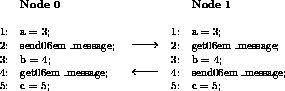
Figure 5.7:
Single-Stepping Through Message-Passing Code
Repeating this process is a problem, however, since we now try to send a
message to node 1 which is not ready to receive it-node 1 is still sitting
in its breakpoint at line one in its node. If we adopted the sequential
debugger standard in which the user program takes control whenever a command
is given to step or continue the program, we would now have a deadlock, because
node 0 will never return from its single-step command until node 1 does
something. On the other hand node 1 cannot do anything until it is given a
debugger command.
In principle, we can get around this problem by redefining the action of the
send_message
function used in node 0. In the normal definition of
our system at that time, this call should block until the receiving node is
ready. By relaxing this constraint, we can allow the
send_message
function to return as soon as the data to be transmitted is safely reusable,
without waiting for the receive.
This does not save the debugger. We now expect the single step from line two
to line three to return, as will the trivial step to line four. But the
single step to line five involves receiving a message from node 1 and
no possible relaxing of the communication specification can deal with
the fact that node 1 hasn't sent anything.
Deadlock is unavoidable.
The solution to this problem is to simply make debugging a completely
autonomous process which operates independently of the user program.
Essentially, this means that any debugger command immediately returns and
gives the user a new prompt. The single-step command, for example, doesn't
wait for anything important to happen but allows the user to carry on giving
debugger commands even though the user process may be ``hung'' as a
consequence of the single step as shown in Figure
5.7
.
Lesson 1a. Who Gets the Input?
As an immediate consequence of the decision to leave the
debugger in control of the keyboard at all times, we run into the
problem of how to pass input to the program being debugged.
Again, sequential debuggers don't have this problem because the moment you
continue or run the program it takes control of the keyboard and you enter
data in the normal manner. In
ndb
, life is not so simple because if
you start up your code and it prints on the screen
Enter two integers: [I,J]
or some such, you can't actually type the values because they would
be interpreted as debugger commands! One way around this is to have multiple
windows on your workstation; in one you type debugger commands; in the
other, input to your program. Another solution is to have a debugger
command that explicitly switches control to the user program in just the same
way that a sequential debugger would:
ndb
supports both mechanisms.
Lesson 2. Show State
Because the debugger operates in the manner just described,
it becomes very important to give the user a quick way of seeing when
something has really happened. Normal sequential debuggers give you
this feedback by simply returning a prompt whenever the user program
has encountered a breakpoint or terminated. In our case, we provide a
simple command, ``
show state
,'' to allow the user to monitor the
progress of the node program.
As an example, the output when executed on node 0 at line two might be
something like
Node 0: Breakpoint, PC=[foo.c,2]
which shows that the node is stopped at a breakpoint at the
indicated line of a source file named ``
foo.c
''. If we step again, the
debugger gives us back a prompt and a very quick ``
show state
'' command
might now show
Node 0: Running, PC=[send.c, 244]
showing that the node is now running code somewhere inside a source
file called ``
send.c
''. Another similar command would probably show
something like
Node 0: Breakpoint, PC=[foo.c, 3]
indicating that the node had now reached the breakpoint on the next
line. If the delay between the first two ``
show state
'' commands were
too long, you might never see the ``Running'' state at all because the node
will have performed its ``send'' operation and reached line three.
If you continued with this process of single stepping and probing with the
``
show state
'' command, you would eventually get to a state where the
node would show as ``Running'' in the receive function from which it would
never return until node 1 got around to sending its message.
Lesson 3. Sets of Nodes
The simplest applications of a sequential debugger for
parallel programs would be similar to those already seen. Each command
issued by the user to the debugger is executed on a particular node.
Up to now, for example, we have considered only actions on node 0.
Obviously, we can't make much progress in the example code shown in
Figure
5.7
until node 1 moves from its initial breakpoint
at line one.
We might extend the syntax by adding a ``
pick
'' command that lets us, for
example,
pick node 1
and then execute commands there instead of on node 0. This would
clearly allow us to make progress in the example we have been studying. On
the other hand, it is very tedious to debug this way. Even on as few as four
nodes, the sequence
is used frequently and is very painful to type. Running on 512
nodes in this manner is out of the question. The solution adopted for
ndb
is to use ``node sets.'' In this case, the above effect would be
achieved with the command
on all show state
or alternatively

The basic idea is that debugger commands can be applied to more
than a single processor at once. In this way, you can obtain global
information about your program without spending hours typing commands.
In addition to the simple concepts of a single node and ``all'' nodes,
ndb
supports other groups such as contiguous ranges of nodes,
discontinuous ranges of nodes, ``even'' and ``odd'' parity groups, the
``neighbors'' of a particular node, and user-defined sets of nodes
to facilitate the debugging process. For example, the command
on 0, 1, nof 1, even show state
executes the ``
show state
'' command on nodes 0, 1, the
neighbors of node 1, and all ``even parity'' nodes.
Lesson 4. Smart stepping
Once node sets are available to execute commands on multiple
processors, another tricky issue comes up concerning single stepping.
Going back to the example shown in Figure
5.7
, consider
the effect of executing the sequence of commands

starting from the initial state in which both nodes are at a
breakpoint at line one. The intent is fairly obvious-the user wants to
single-step over the intermediate lines of code from line one, eventually
ending up at line five.
In principle, the objections that gave rise to the independence of debugger
and user program should no longer hold, because when we step from line
two, both nodes are participating and thus the send/receive combination
should be satisfied properly.
The problem, however, is merely passed down to the internal logic of
the debugger. While it is true that the user has asked both nodes to
step over their respective communication calls, the debugger is hardly
likely to be able to deduce that. If the debugger expands (internally)
the single-step command to something like

then all might be well, since node 0 will step over its ``send''
before node 1 steps over its receive-a happy result. If, however, the
debugger chooses to expand this sequence as

it will hang just as badly as the original user interaction.
Even though the ``obvious'' expansion is the one that works in this case,
this is not generally true-in fact, it fails when stepping from line four to
line five in the example.
In general, there is no way for the debugger to know how to expand such
command sequences reliably, and as a result a much ``smarter'' method of
single stepping must be used, such as that shown schematically in
Figure
5.8
.
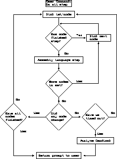
Figure 5.8:
Logic for Single Stepping on Multiple Nodes
The basic idea is to loop over each of the nodes in the set being stepped
trying to make ``some'' progress towards reaching the next stopping point.
If no nodes can make progress, we check to see if some time-out has expired
and if not, continue. This allows us to step over system calls that may
take a significant time to complete when measured in machine instructions.
Finally, if no more progress can be made, we attempt to analyze the reason for
the deadlock and return to the user anyway.
This process is not foolproof in the sense that we will sometimes
``give up'' on single steps that are actually going to complete, albeit
slowly. But it has the great virtue that even when the user program
``deadlocks'', the debugger comes back to the user, often with a
correct analysis of the reason for the deadlock.
Lesson 5. Show queue
Another interesting question about the debugger concerns the
extensions and/or modifications that one might make to a sequential
debugger.
One might be tempted to say that the parallel debugger is so different from
its sequential counterparts that a totally new syntax and method of operation
is justified. One then takes the chance that no one will invest the time
needed to learn the new tool and it will never be useful.
For
ndb
, we decided to adopt the syntax of the well-known UNIX
dbx
debugger that
was available on the workstations that we used for development. This meant
that the basic command syntax was familiar to everyone using the system.
Of course we have already introduced several commands that don't exist
in
dbx
, simply because sequential debuggers don't have need for them.
The ``
show state
'' command is never required in sequential
debuggers because the program is either running or it's stopped at a
point that the debugger can tell you about. Similarly, one never has
to give commands to multiple processors.
Another command that we learned early on was very important was ``
show q
'', which monitored the messages in transit between processors.
Because our parallel programs were really just sequential programs with
additional message passing, the ``bugs'' that we were trying to find
were not normally algorithmic errors but message-passing ones.
A typical scenario would be that the nodes would compute (correctly) and then
reach some synchronization or communication point at which point the logic
relating to message transfer would be wrong and everything would hang. At
this point, it proved to be immensely useful to be able to go in with the
debugger and look at which nodes had actually sent messages to other nodes.
Often one would see something like
Node 0:
Node 1, type 12, len 32
(12 4a 44 82 3e 00 ...)
Node 2, type 12, len 32
(33 4a 5f ff 00 00 ...)
Node 1: No messages
Node 2: No messages
indicating that node 0 has received two messages of type 12 and
length 32 bytes from node 1 and node 2 but that neither node 1 nor node 2 has
any.
Armed with this type of information, it is usually extremely easy to detect
the commonest type of parallel processing problem.
Lesson 5a. Message Passing Is Easy
An interesting corollary to the debugging style just
described is that we learned that debugging message-passing programs
was
much
easier than other types of parallel programming.
The important advantage that a user-friendly debugger brings to the
user is the ability to slow down the execution of the program to the
point where the user can ``see'' the things that go wrong. This fits
well with the ``message-passing'' methodology since bugs in message
passing usually result in the machine hanging. In this state, you have
plenty of time to examine what's happening and deduce the error.
Furthermore, the problem is normally completely repeatable since it
usually relates to a logic error in the code.
In contrast, shared-memory or multiprocessing paradigms are much harder
because the bugs tend to depend on the relative timing of various events
within the code. As a result, the very act of using the debugger can cause
the problem to show up in a different place or even to go away all together.
This is akin to that most frustrating of problems when you are tracking down
a bug with print statements, only to find that just as you insert the
climactic final statement which will isolate your problem, it goes away
altogether!
Lesson 6. How Many Windows?
The debugger
ndb
was originally designed to be driven
from a terminal by users typing commands, but with the advent of
graphical workstations with windowing systems it was inevitable that
someone would want a ``windowing'' version of the debugger.
It is interesting to note that many users' original conception was that it
would now be correct to port a sequential debugger and have multiple
instances of it, each debugging one node.
This illusion is quickly removed, however, when we are debugging a program on
many nodes with many invocations of a sequential debugger. Not only is it
time-consuming setting up all of the windows, but activities such as single
stepping become extremely frustrating since one has to go to each window in
turn and type the ``continue'' command. Even providing a ``button'' that can
be clicked to achieve this doesn't help much because you still have to be
able to see the button in the overlapping windows, and however fast you are
with the mouse it gets harder and harder to achieve this effect as the number
of nodes on which your program is running grows.
Our attempt at solving this problem is to have two different window
types: an
ndb
console and a node window. The console is
basically a window-oriented version of the standard debugger. The
lower panel allows the user to type any of the normal debugger commands
and have them behave in the expected fashion. The buttons at the top
of the display allow ``shortcuts'' for the often issued commands, and
the center panel allows a shortcut for the most popular command of all:
on all show state
This button doesn't actually generate the output from this command
in the normal mode since, brief as its output is, it can still be tedious
watching 512 copies of
Node XXX: Breakpoint, [foo.c, 13]
scroll past. Instead, it presents the node state as a colored bar
chart in which the various node states each have different colors. In this
way, for example, you can ``poll'' until all the nodes hit a breakpoint by
continually hitting the ``
Update
'' button until the status panel shows
a uniform color and the message shows that all nodes have reached a
breakpoint.
In addition to this usage, the color coding also vividly shows problems such
as a node dividing by zero. In this case, the bar chart would show uniform
colors except for the node that has died, which might show up in some
contrasting shade.
The second important use of the ``
Update
'' button is to synchronize the
views presented by the second type of window, the ``node windows.''
Each of these presents a view of a ``group'' of nodes represented by a
particular choice. Thus, for example, you might choose to make a node window
for the nodes 0-3, represented by node 0. In this case, the upper panel of
the node window would show the source code being executed by node 0 while the
lower panel would automatically direct commands to all four nodes in the
group. The small status bar in the center shows a ``smiley'' face if all
nodes in the group appear to be at the same source line number and a
``sad'' face if one or more nodes are at different places.
This method allows the user to control large groups of nodes and
simultaneously see their source code while also monitoring differences in
behavior. A common use of the system, for example, is to start with a single
node window reflecting ``all nodes'' and to continue in this way until
the happy face becomes sad, at which point additional node windows can be
created to monitor those nodes which have departed from the main thread of
execution.
The importance of the ``
Update
'' button in this regard is that the
node windows have a tendency to get out of sync with the actual
execution of the program. In particular, it would be prohibitively expensive
to have each node window constantly tracking the program location of the
nodes it was showing, since this would bombard the node program with status
requests and also cause constant scrolling of the displayed windows.
Instead,
ndb
chooses its own suitable points to update the
displayed windows and can be forced to update them at other times with the
``
Update
'' button.
Next:
5.3.3 Conclusions
Up:
5.3 Parallel Debugging
Previous:
5.3.1 Introduction and History
Guy Robinson
Wed Mar 1 10:19:35 EST 1995
5.3.3 Conclusions
Next:
5.4 Parallel Profiling
Up:
5.3 Parallel Debugging
Previous:
5.3.2 Designing a Parallel
This section has emphasized the differences between
ndb
and
sequential debuggers since those are the interesting features from the
implementation standpoint. On the other hand, from the user's view, the most
striking success of the tool is that it has made the debugging process so
little different from that used on sequential codes. This can be
traced to the loosely synchronous structure of most (C P) parallel
codes. Debugging fully asynchronous parallel codes can be much more
challenging than the sequential case.
P) parallel
codes. Debugging fully asynchronous parallel codes can be much more
challenging than the sequential case.
In practice, users have to be shown only once how to start up the debugging
process, and be given a short list of the new commands that they might want to
use. For users who are unfamiliar with the command syntax, the simplest
route is to have them play with
dbx
on a workstation for a few minutes.
After this, the process tends to be very straightforward, mostly because of
the programming styles that we tend to use. As mentioned in an earlier
section, debugging totally asynchronous programs that generate multiple
threads synchronizing with semaphores in a time-dependent manner is not
ndb
's forte. On the other hand, debugging loosely synchronous
message-passing programs has been reduced to something of a triviality.
In some sense, we can hardly be said to have introduced anything new. The
basis on which
ndb
operates is very conventional, although some of the
implications for the implementation are non-trivial. On the other hand, it
provides an important and often critical service to the user. The next
section will describe some of the more revolutionary steps that were
taken to simplify the development process in the areas of performance
analysis
and
visualization.
Guy Robinson
Wed Mar 1 10:19:35 EST 1995
5.4 Parallel Profiling
Next:
5.4.1 Missing a Point
Up:
Express and CrOS
Previous:
5.3.3 Conclusions
From the earliest days of parallel computing, the fundamental goal was to
accelerate the performance of algorithms that ran too slowly on sequential
machines. As has been described in many other places in this book, the
effort to do basic research in computer science was always secondary to the
need for algorithms that solved practical problems more quickly than was
possible on other machines.
One might think that an important prerequisite for this would be advanced
profiling technology. In fact, about the most advanced piece of equipment
then in use was a wristwatch! Most algorithms were timed on one node, then
on two, then on four, and so on. The results of this analysis were then compared
with the theoretically derived models for the applications. If all was well,
one proceeded to number-crunch; if not, one inserted print statements and
timed the gaps between them to see what pieces of code were behaving in ways
not predicted by the models.
Even the breakthrough of having a function that a program could call to get
at timing information was a long time coming, and even then proved somewhat
unpopular, since it had different names on different machines and didn't
even exist on the sequential machines. As a result, people tended to just
not bother with it rather than mess up their codes with many different timing
routines.
Guy Robinson
Wed Mar 1 10:19:35 EST 1995
5.4.1 Missing a Point
Next:
5.4.2 Visualization
Up:
5.4 Parallel Profiling
Previous:
5.4 Parallel Profiling
Of course, this was all totally adequate for the first few applications that
were parallelized, since their behavior was so simple to model. A program
solving Laplace's
equation on a square grid, for
example, has a very simple model that one would actually have to work
quite hard not to find in a parallel code. As time passed, however,
more complex problems were attempted which weren't so easy to model and
tools had to be invented.
Of course, this discussion has missed a rather important point which we also
tended to overlook in the early days.
When comparing performance of the problems on one, two, four, eight,
and so on nodes, one is really only assessing the efficiency of the
parallel version of the code. However, an algorithm that achieves
100 percent efficiency on a parallel computer may still be worthless if
its absolute performance is lower than that of a sequential code
running on another machine.
Again, this was not so important in the earliest days, since the big battle
over architectures had not yet arisen. Nowadays, however, when there is a
multitude of sequential and parallel supercomputers, it is extremely important
to be able to know that a parallel version of a code is going to outperform a
sequential version running on another architecture. It is becoming
increasingly important to be able to understand what complex algorithms
are doing and why, so that the performance of the software and hardware can
both be tuned to achieve best results.
This section attempts to discuss some of the issues surrounding
algorithm visualization, parallelization and performance
optimization,
and the tools which C P developed
to help in this area. A major recent general tool, PABLO
[
Reed:91a
] has been developed at Illinois by Reed's group, but
here we only describe the C
P developed
to help in this area. A major recent general tool, PABLO
[
Reed:91a
] has been developed at Illinois by Reed's group, but
here we only describe the C P activity. One of the earliest tools
was Seecube [Couch:88a;88b].
P activity. One of the earliest tools
was Seecube [Couch:88a;88b].
Next:
5.4.2 Visualization
Up:
5.4 Parallel Profiling
Previous:
5.4 Parallel Profiling
Guy Robinson
Wed Mar 1 10:19:35 EST 1995
5.4.2 Visualization
Next:
5.4.3 Goals in Performance
Up:
5.4 Parallel Profiling
Previous:
5.4.1 Missing a Point
The first question that must be asked of any algorithm when a parallel
version is being considered is, ``What does it do?'' Surprisingly, this
question is often quite hard to answer. Vague responses such as ``some sort
of linear algebra'' are quite common and even if the name of the algorithm
is actually known, it is quite surprising how often codes are ported without
anyone actually having a good impression of what the code does.
One attempt to shed light on these issues by providing a data visualization
service is
vtool
. One takes the original (sequential) source code
and runs it through a preprocessor that instruments various types of data
access. The program is then compiled with a special run time library and run
in the normal manner. The result is a database describing the ways in which
the algorithm or application makes use of its data.
Once this has been collected,
vtool
provides a service analogous to
a home VCR which allows the application to be ``played back'' to show the
memory accesses being made. Sample output is shown in
Figure
5.9
.
Figure 5.9:
Analysis of a Sorting Algorithm Using
vtool
The basic idea is to show ``pictures'' of arrays together with a ``hot spot''
that shows where accesses and updates are being made. As the hot spot moves,
it leaves behind a trail of continuingly fading colors that dramatically show
the evolution of the algorithm. As this proceeds, the corresponding source
code can be shown and the whole simulation can be stopped at any time so that
a particularly interesting sequence can be replayed in slow motion or even
one step at a time, both forward and backward.
In addition to showing simple access patterns, the display can also show the
values being stored into arrays, providing a powerful way of debugging
applications.
In the parallel processing arena, this tool is normally used to understand
how an algorithm works at the level of its memory references. Since most
parallel programs are based on the ideas of data distribution, it is
important to know how the values at a particular grid point or location in
space depend on those of neighbors. This is fundamental to the selection of
a parallelization method. It is also central to the understanding of how the
parallel and sequential versions of the code will differ which becomes
important when the optimization process begins.
It should be mentioned in passing that we have been surprised in using this
tool how often people's conceptions of the way that numerical algorithms work
are either slightly or completely revised after seeing the visualization
system at work.
Next:
5.4.3 Goals in Performance
Up:
5.4 Parallel Profiling
Previous:
5.4.1 Missing a Point
Guy Robinson
Wed Mar 1 10:19:35 EST 1995
5.4.3 Goals in Performance Analysis
Next:
5.4.4 Overhead Analysis
Up:
5.4 Parallel Profiling
Previous:
5.4.2 Visualization
Hopefully, the visualization system goes some way towards the development
of a parallel algorithm. One must then code and debug the application which,
as has been described previously, can be a reasonably time-consuming process.
Finally, one comes to the ``crisis'' point of actually running the parallel
code and seeing how fast it goes.
One of our major concerns in developing performance
analysis
tools was
to make them easy to use. The standard UNIX method of taking the
completed program, deleting all its object files, and then recompiling
them with special switches seemed to be asking too much for parallel
programs because the process is so iterative. On a sequential machine,
the profiler may be run once or twice, usually just to check that the
authors' impressions of performance are correct. On a parallel
computer, we feel that the optimization phase should more correctly be
included in the development cycle than as an afterthought, because we
believe that few parallel applications perform at their best
immediately after debugging
is complete. We wanted,
therefore, to have a system that could give important information about
an algorithm without any undue effort.
The system to be described works with the simple addition of either a runtime
switch or the definition of an ``environment'' variable, and makes available
about 90% of the capabilities of the entire package. To use some of the
most exotic features, one must recompile code.
Guy Robinson
Wed Mar 1 10:19:35 EST 1995
5.4.4 Overhead Analysis
Next:
5.4.5 Event Tracing
Up:
5.4 Parallel Profiling
Previous:
5.4.3 Goals in Performance
As an example of the ``free'' profiling information that is available
consider the display from the
ctool
utility shown in
Figure
5.10
. This provides a summary of the gross
``overheads'' incurred in the execution of a parallel application
divided into categories such as ``calculation,'' ``I/O,'' ``internode
communication,'' ``graphics,'' and so on. This is the first type of
information that is needed in assessing a parallel program and is
obtained by simply adding a command line argument to an existing
program.
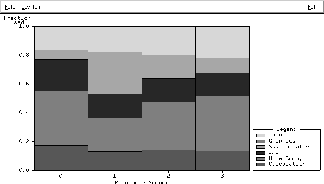
Figure 5.10:
Overhead Summary from
ctool
At the next level of detail after this, the individual overhead categories
can be broken down into the functions responsible for them. Within the
``internode communication'' category, for example, one can ask to be shown
the times for each of the high-level communication functions, the number of
times each was called and the distribution of message lengths used by each.
This output is normally presented graphically, but can also be generated in
tabular form (Figure
5.11
) for accurate timing measurements.
Again, this information can be obtained more or less ``for free'' by giving a
command line argument.
Figure 5.11:
Tabular Overhead Summary
Guy Robinson
Wed Mar 1 10:19:35 EST 1995
5.4.5 Event Tracing
Next:
5.4.6 Data Distribution Analysis
Up:
5.4 Parallel Profiling
Previous:
5.4.4 Overhead Analysis
The overhead summaries just described offer replies to the important question,
``What are the costs of executing this algorithm in parallel?'' Once
this information is known, one typically proceeds to the question, ``Why do
they cost this much?''
To answer this question we use
etool
, the event-tracing profiler.
The purpose of this tool is probably most apparent from its sample
output, Figure
5.12
. The idea is that we present
timelines for each processor on which the most important ``events'' are
indicated by either numbered boxes or thin bars. The former indicate
atomic
events such as ``calling subroutine
foo
'' or
``beginning of loop at line 12,'' while the bars are used to indicate
the beginning and end of extended events such as a read operation on a
file or a global internode communication operation.
Figure 5.12:
Simple Event Traces
The basic idea of this tool is to help understand why the various
overheads observed in the previous analysis exist. In particular, one looks
for behavior that doesn't fit with that expected of the algorithm.
One common situation, for example, is to look for places where a
``loosely synchronous'' operation is held up by the late arrival of one
or more processors at the synchronization point. This is quite simple
in
etool
; an ``optimal'' loosely synchronous
event would have bars in each processor that aligned
perfectly in the vertical direction. The impact of a late processor
shows up quite vividly, as shown in Figure
5.13
.
Figure 5.13:
Sample Application Behavior as Seen by
etool
This normally occurs either because of a poorly constructed algorithm or
because of poor load balancing due to data dependencies.
An alternative pattern that shows up remarkably well is the sequential
behavior of ``master-slave'' or ``client-server'' algorithms in which one
particular node is responsible for assigning work to a number of other
processors. These algorithms tend to show patterns similar to that of
Figure
5.12
, in which the serialization of the loop that
distributed work is quite evident.
Another way that the event-profiling system can be used is to collect
statistics regarding the usage of particular code segments. Placing calls to
the routine
eprof_toggle
around a particular piece of code causes
information to be gathered describing how many times that block was executed,
and the mean and variance of the time spent there. This is analogous to the
``block profiling'' supported by some compilers.
Next:
5.4.6 Data Distribution Analysis
Up:
5.4 Parallel Profiling
Previous:
5.4.4 Overhead Analysis
Guy Robinson
Wed Mar 1 10:19:35 EST 1995
5.4.6 Data Distribution Analysis
Next:
5.4.7 CPU Usage Analysis
Up:
5.4 Parallel Profiling
Previous:
5.4.5 Event Tracing
The system first described,
vtool
, had as its goal the visualization of
sequential programs prior to their parallelization. The distribution profiler
dtool
serves a similar purpose for parallel programs which
rely on data distribution for their parallelism. The basic idea is that one
can ``watch'' the distribution of a particular data object change as an
algorithm progresses. Sample output is shown in Figure
5.14
.
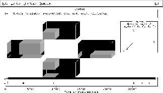
Figure 5.14:
Data Distribution Analysis
At the bottom of the display is a timeline which looks similar to that used
in the event profiler,
etool
. In this case, however, the events shown
are the redistribution operations on a particular data object. Clicking on
any event with the mouse causes a picture of the data distribution among the
nodes to be shown in the upper half of the display. Other options allow
for fast and slow replays of a particular sequence of data transformations.
The basic idea of this tool is to look at the data distributions that are
used with a view to either optimizing their use or looking for places in
which redundant transformations are being made that incur high communication
costs. Possible restructuring of the code may eliminate these transformations,
thus improving performance. This is particularly useful in conjunction with
automatic parallelization tools, which have a tendency to insert redundant
communication in an effort to ensure program correctness.
Guy Robinson
Wed Mar 1 10:19:35 EST 1995
5.4.7 CPU Usage Analysis
Next:
5.4.8 Why So Many
Up:
5.4 Parallel Profiling
Previous:
5.4.6 Data Distribution Analysis
As mentioned earlier, the most often neglected question with parallel
applications is how fast they are in absolute terms. It is possible that
this is a throwback to sequential computers, where profiling tools, although
available, are rarely used. In most cases, if a program doesn't run fast
enough when all the compiler's optimization capabilities are exhausted, one
merely moves to a higher performance machine. Of course, this method doesn't
scale well and doesn't apply at all in the supercomputer arena. Even more
importantly, as processor technology becomes more and more complex, the
performance gap between the peak speed of a system and that attained by
compiled code gets ever wider.
The typical solution for sequential computers is the use of
profiling
tools like
prof
or
gprof
that provide a tabular listing of the routines in a program and the
amount of time spent in each. This avoids the use of the wristwatch
but only goes so far. You can certainly see which routines are the
most expensive but no further.
The profiler
xtool
was designed to serve this purpose for
parallel computers and in addition to proceed to lower levels of
resolution: source code and even machine instructions. Sample
displays are shown in Figure
5.15
. At the top is a
graphical representation of the time spent executing each of the most
expensive routines. The center shows a single routine at the level of
its source code and the bottom panel shows individual machine
instructions.
Figure 5.15:
Output from the CPU Usage Profiler
The basic goal of this presentation is to allow the user to see where CPU
time is being spent at any required level of detail. At the top level, one
can use this information to develop or restructure algorithms, while at the
lowest level one can see how the processor instructions operate and
use this data to rework pieces of code in optimized assembly language.
Note that while the other profiling tools are directed specifically towards
understanding the parallel processing issues of an application, this tool is
aimed mostly at a thorough understanding of sequential behavior.
Next:
5.4.8 Why So Many
Up:
5.4 Parallel Profiling
Previous:
5.4.6 Data Distribution Analysis
Guy Robinson
Wed Mar 1 10:19:35 EST 1995
5.4.8 Why So Many Separate Tools?
Next:
5.4.9 Conclusions
Up:
5.4 Parallel Profiling
Previous:
5.4.7 CPU Usage Analysis
One of the most often asked questions about this profiling system is why
there are so many separate tools rather than an all-encompassing system that
tells you everything you wish to know about the application.
Our fundamental reason for choosing this method was to attempt to minimize
the ``self-profiling'' problem that tends to show up in many systems in which
the profiling activity actually spends most of its time profiling the analysis
system itself. Users of the UNIX profiling tools, for example, have become
adept at ignoring entries for routines such as
mcount
, which
correspond to time spent within the profiling system itself.
Unfortunately, this is not so simple in a parallel program. In sequential
applications, the effect of the profiling system is merely to slow down other
types of operation, an effect which can be compensated for by merely
subtracting the known overheads of the profiling operations. On a parallel
computer, things are much more complicated, since slowing down one processor
may affect another which in turn affects another, and so on until the whole
system is completely distorted by the profiling tools.
Our approach to this problem is to package up the profiling subsystems in
subsets which have more or less predictable effects, and then to let the user
decide which systems to use in which cases. For example, the communication
profiler,
ctool
, incurs very small overheads-typically a fraction
of 1%-while the event profiler costs more and the CPU usage
profiler,
xtool
, most of all. In common use, therefore, we tend to use
the communication profiler first, and then enable the event traces. If these
two trials yield consistent results, we move on to the execution and
distribution profilers. We have yet to encounter an application in which
this approach has failed, although the fact that we are rarely interested in
microsecond accuracy helps in this regard.
Interestingly, we have found problems due to ``clock-skewing'' to have
negligible impact on our results. It is true that clock skewing occurs in
most parallel systems, but we find that our profiling results are accurate
enough to be helpful without taking any special precautions in this regard.
Again, this is mostly due to the fact that, for the kinds of performance
analysis and optimization in which we are interested, resolution of tens or
even hundreds of microseconds is usually quite acceptable.
Next:
5.4.9 Conclusions
Up:
5.4 Parallel Profiling
Previous:
5.4.7 CPU Usage Analysis
Guy Robinson
Wed Mar 1 10:19:35 EST 1995
5.4.9 Conclusions
Next:
6 Synchronous Applications II
Up:
5.4 Parallel Profiling
Previous:
5.4.8 Why So Many
Our assumption that parallel algorithms are complex entities seems to be
borne out by the fact that nearly everyone who has invested the (minimal)
time to use the profiling tools on their application has come away
understanding something better than before. In some cases, the revelations
have been so profound that significant performance enhancements have been
made possible.
In general, the system has been found easy to use, given a basic understanding
of the parallel algorithm being profiled, and most users have no difficulty
recognizing their applications from the various displays. On the other hand,
the integration between the different profiling aspects is not yet as tight
as one might wish and we are currently working on this aspect.
Another interesting issue that comes up with great regularity is the request
on behalf of the users for a button marked ``Why?'', which would
automatically analyze the profile data being presented and then point out a
block of source code and a suggestion for how to improve its performance.
In general, this is clearly too difficult, but it is interesting to note that
certain types of runtime system are more amenable to this type of analysis
than others. The ``distribution profiler,'' for instance, possesses
enough information to perform quite complex communication and
I/O
optimizations on an algorithm and we are currently
exploring ways of implementing these strategies. It is possible that
this line of thought may eventually lead us to a more complete
programming model than is in use now-one which will be more amenable
to the automation of parallel processing that has long been our goal.
Guy Robinson
Wed Mar 1 10:19:35 EST 1995
6 Synchronous Applications II
Next:
6.1 Computational Issues
in
Up:
Parallel Computing Works
Previous:
5.4.9 Conclusions
Guy Robinson
Wed Mar 1 10:19:35 EST 1995
6.1 Computational Issues
in SynchronousProblems
Next:
Convectively-Dominated Flows and
Up:
6 Synchronous Applications II
Previous:
6 Synchronous Applications II
Synchronous problems have been defined in Section
3.4
as
having the simplest temporal or computational structure. The problems
are typically defined by a regular grid, as illustrated in
Figure
4.3
, and are parallelized by a simple domain
decomposition. A synchronous temporal structure
corresponds to each point in the data domain being evolved
with an identical computational algorithm, and we summarize this in the
caricature shown in Figure
6.1
. We find several
important synchronous problems in the academic applications, which
formed the core of C P's work. We expect-as shown in
Chapter
19
-that the ``real world'' (industry and government)
will show fewer problems of the synchronous class. One hopes that a
fundamental theory will describe phenomena in terms of simple elegant
and uniform laws; these are likely to lead to a synchronous or
computational (temporal) structure. On the other hand, real-world
problems typically involve macroscopic phenomenological models as
opposed to fundamental theories of the microscopic world.
Correspondingly, we find in the real world more loosely synchronous
problems that only exhibit macroscopic temporal synchronization.
P's work. We expect-as shown in
Chapter
19
-that the ``real world'' (industry and government)
will show fewer problems of the synchronous class. One hopes that a
fundamental theory will describe phenomena in terms of simple elegant
and uniform laws; these are likely to lead to a synchronous or
computational (temporal) structure. On the other hand, real-world
problems typically involve macroscopic phenomenological models as
opposed to fundamental theories of the microscopic world.
Correspondingly, we find in the real world more loosely synchronous
problems that only exhibit macroscopic temporal synchronization.
Figure 6.1:
The Synchronous Problem Class
There is no black-and-white definition of synchronous since, practically,
we allow some violations of the rigorous microscopic synchronization.
This is already seen in Section
4.2
's discussion of the
irregularity of Monte Carlo
``accept-reject''
algorithms. A deeper example is irregular geometry problems, such as
the partial differential equations of Chapters
9
and
12
with an irregular mesh. The simplest of these can be
implemented well on SIMD machines as long as each node can access
different addresses. In the High Performance Fortran analysis of
Chapter
13
, there is a class of problems lacking the regular
grid of Figure
4.3
. They cannot be expressed in terms of
Fortran 90 with arrays of values. However, the simpler irregular
meshes are topologically rectangular-they can be expressed in
Fortran 90 with an array of pointers. The SIMD Maspar
MP-1,2 supports this node-dependent addressing and has termed this an
``autonomous SIMD'' feature. We believe that just as SIMD is not a
precise computer architecture, the synchronous problem class will also
inevitably be somewhat vague, with some problems having architectures
in a grey area between synchronous and loosely synchronous.
The applications described in Chapter
4
were all run on MIMD
machines using the message-passing model of Chapter
5
.
Excellent speedups were obtained. Interestingly, even when C P
acquired a SIMD CM-2, which also supported this problem class well, we
found it hard to move onto this machine because of the different
software model-the data parallel languages of
Chapter
13
-offered by SIMD machines. The development of High
Performance Fortran, reviewed in Section
13.1
, now offers the same
data-parallel programming model on SIMD and MIMD machines for
synchronous problems. Currently, nobody has efficiently ported the
message-passing model to SIMD machines-even with the understanding
that it would only be effective for synchronous problems. It may be
that with the last obvious restriction, the message-passing model could
be implemented on SIMD machines.
P
acquired a SIMD CM-2, which also supported this problem class well, we
found it hard to move onto this machine because of the different
software model-the data parallel languages of
Chapter
13
-offered by SIMD machines. The development of High
Performance Fortran, reviewed in Section
13.1
, now offers the same
data-parallel programming model on SIMD and MIMD machines for
synchronous problems. Currently, nobody has efficiently ported the
message-passing model to SIMD machines-even with the understanding
that it would only be effective for synchronous problems. It may be
that with the last obvious restriction, the message-passing model could
be implemented on SIMD machines.
This chapter includes a set of neural network
applications. This is an important class of naturally parallel
problems, and represents one approach to answering the question:
``How can one apply massively parallel machines to artificial
intelligence
(AI)?''
We were asked this many times at the start of C P, since AI was one of
the foremost fields in computer science at the time. Today, the
initial excitement behind the Japanese fifth-generation project has
abated and AI has transitioned to a routine production technology which
is perhaps more limited than originally believed. Interestingly, the
neural network approach leads to synchronous structure, whereas the
complementary actor or expert system approaches have a very
different asynchronous structure.
The high temperature superconductivity
calculations in
Section
6.3
made a major impact on the condensed matter
community. Quoting from
Nature
[
Maddox:90a
]
P, since AI was one of
the foremost fields in computer science at the time. Today, the
initial excitement behind the Japanese fifth-generation project has
abated and AI has transitioned to a routine production technology which
is perhaps more limited than originally believed. Interestingly, the
neural network approach leads to synchronous structure, whereas the
complementary actor or expert system approaches have a very
different asynchronous structure.
The high temperature superconductivity
calculations in
Section
6.3
made a major impact on the condensed matter
community. Quoting from
Nature
[
Maddox:90a
]
``Yet some progress seems to have been made. Thus Hong-Qiang Ding and
Miloje S. Makivic, from California Institute of Technology, now
describe an exceedingly powerful Monte Carlo
calculation of an antiferromagnetic lattice designed to allow for the
simulation of  (
Phys. Rev. Lett.
64
,
1,449; 1990). In this context, a Monte Carlo simulation entails
starting with an arbitrary arrangement of spins on the lattice, and
then changing them in pairs according to rules that allow all spin
states to be reached without violating the overall constraints. The
authors rightly boast of their access to Caltech's parallel computer
system, but they have also devised a new and efficient algorithm for
tracing out the evolution of their system. As is the custom in this
part of the trade, they have worked with square patches of
two-dimensional lattice with as many as 128 lattice spacings to each
side.
(
Phys. Rev. Lett.
64
,
1,449; 1990). In this context, a Monte Carlo simulation entails
starting with an arbitrary arrangement of spins on the lattice, and
then changing them in pairs according to rules that allow all spin
states to be reached without violating the overall constraints. The
authors rightly boast of their access to Caltech's parallel computer
system, but they have also devised a new and efficient algorithm for
tracing out the evolution of their system. As is the custom in this
part of the trade, they have worked with square patches of
two-dimensional lattice with as many as 128 lattice spacings to each
side.
The outcome is a relationship between correlation length-the
distance over which order, on the average, persists-and
temperature; briefly, the logarithm of the correlation length is
inversely proportional to the temperature. That, apparently,
contradicts other models of the ordering process. In lanthanum copper
oxide, the correlation length agrees well with that measured by
neutron diffraction below  (where there is a phase
transition), provided the interaction energy is chosen appropriately.
For what it is worth, that energy is not very different from estimates
derived from Raman-scattering experiments, which provide a direct
measurement of the energy of interaction by the change of frequency of
the scattered light.''
(where there is a phase
transition), provided the interaction energy is chosen appropriately.
For what it is worth, that energy is not very different from estimates
derived from Raman-scattering experiments, which provide a direct
measurement of the energy of interaction by the change of frequency of
the scattered light.''
The hypercube allowed much larger high- calculations than the
previous state of the art, with conventional machines. Curiously,
with QCD simulations (described in Section
4.3
), we were only
able at best to match the size of the Cray
calculations of other
groups. This probably reflects different cultures and computational
expectations of the QCD and condensed matter
communities. C
calculations than the
previous state of the art, with conventional machines. Curiously,
with QCD simulations (described in Section
4.3
), we were only
able at best to match the size of the Cray
calculations of other
groups. This probably reflects different cultures and computational
expectations of the QCD and condensed matter
communities. C P had the advantage of dedicated facilities and
could devote them to the most interesting applications.
P had the advantage of dedicated facilities and
could devote them to the most interesting applications.
Section
6.2
describes an early calculation, which was a
continuation of our collaboration with Sandia on nCUBE
applications. They, of course, followed this with a major internal
activity, including their impressive performance analysis
of 1024-node applications
[
Gustafson:88a
]. There were several other synchronous
applications in C P that we will not describe in this book. Wasson
solved the single-particle Schrödinger equation in a regular grid to
study the ground state of nuclear matter
as a
function of temperature and pressure. His approach used the
time-dependent Hartree-Fock method, but was never taken past the stage
of preliminary calculations on the early Mark II machines
[
Wasson:87a
]. There were also two interesting signal-processing
algorithms. Pollara implemented the Viterbi
algorithm
for convolutional
decoding of data sent on noisy
communication channels [
Pollara:85a
], [
Pollara:86a
]. This
has similarities with the Cooley-Tukey binary FFT
parallelization described in [
Fox:88a
]. We also looked at
alternatives to this binary FFT in a collaboration with Aloisio from
the Italian Space Agency. The prime number (nonbinary) discrete
Fourier transform produces a more irregular communication pattern than
the binary FFT and, further, the node calculations are less easy to
pipeline than the conventional FFT. Thus, it is hard to achieve the
theoretical advantage of the nonbinary FFT. This often has less
floating-point operations needed for a given analysis whose natural
problem size may not be the power of two demanded by the binary FFT
P that we will not describe in this book. Wasson
solved the single-particle Schrödinger equation in a regular grid to
study the ground state of nuclear matter
as a
function of temperature and pressure. His approach used the
time-dependent Hartree-Fock method, but was never taken past the stage
of preliminary calculations on the early Mark II machines
[
Wasson:87a
]. There were also two interesting signal-processing
algorithms. Pollara implemented the Viterbi
algorithm
for convolutional
decoding of data sent on noisy
communication channels [
Pollara:85a
], [
Pollara:86a
]. This
has similarities with the Cooley-Tukey binary FFT
parallelization described in [
Fox:88a
]. We also looked at
alternatives to this binary FFT in a collaboration with Aloisio from
the Italian Space Agency. The prime number (nonbinary) discrete
Fourier transform produces a more irregular communication pattern than
the binary FFT and, further, the node calculations are less easy to
pipeline than the conventional FFT. Thus, it is hard to achieve the
theoretical advantage of the nonbinary FFT. This often has less
floating-point operations needed for a given analysis whose natural
problem size may not be the power of two demanded by the binary FFT
[Aloisio:88a;89b;90b;91a;91b]. This parallel discrete FFT was designed
for synthetic aperture radar applications for the analysis of satellite
data [Aloisio:90c;90d].
The applications in Sections
6.7.3
,
6.5
, and
6.6
use the important multiscale
approach to a
variety of vision or image processing
problems. Essentially, all physical problems are usefully considered
at several different length scales, and we will come back to this in
Chapters
9
and
12
when we study partial differential
equations (multigrid) and practice dynamics (fast multipole).
Next:
Convectively-Dominated Flows and
Up:
6 Synchronous Applications II
Previous:
6 Synchronous Applications II
Guy Robinson
Wed Mar 1 10:19:35 EST 1995
Convectively-Dominated Flows and
theFlux-Corrected Transport Technique
Next:
6.2.1 An Overview of
Up:
6 Synchronous Applications II
Previous:
6.1 Computational Issues
in
This work implemented a code on the nCUBE-1 hypercube for studying the
evolution of two-dimensional, convectively-dominated fluid
flows. An explicit finite difference
scheme
was used that incorporates the flux-corrected transport
(FCT)
technique developed by Boris and Book
[
Boris:73a
]. When this work was performed in 1986-1987, it was
expected that explicit finite difference schemes for solving partial
differential equations would run efficiently on MIMD distributed-memory
computers, but this had only been demonstrated in practice for ``toy''
problems on small hypercubes of up to 64 processors. The motivation
behind this work was to confirm that a bona fide scientific application
could also attain high efficiencies on a large commercial hypercube.
The work also allowed the capabilities and shortcomings of the
newly-acquired nCUBE-1 hypercube to be assessed.
Other References and Paradigms
HPFA Applications and Paradigms
Guy Robinson
Wed Mar 1 10:19:35 EST 1995
6.2.1 An Overview of the FCT Technique
Next:
6.2.2 Mathematics and the
Up:
Convectively-Dominated Flows and
Previous:
Convectively-Dominated Flows and
Although first-order finite difference methods are monotonic and stable,
they are also strongly dissipative, causing the solution to become smeared
out. Second-order techniques are less dissipative, but are susceptible to
nonlinear, numerical instabilities that cause nonphysical oscillations in
regions of large gradient. The usual way to deal with these types of
oscillation is to incorporate artificial diffusion into the numerical
scheme. However, if this is applied uniformly over the problem domain,
and enough is added to dampen spurious oscillations in regions of large
gradient, then the solution is smeared out elsewhere. This difficulty is
also touched upon in Section
12.3.1
. The FCT technique is a scheme
for applying artificial diffusion to the numerical solution of a
convectively-dominated flow problem in a spatially nonuniform way. More
artificial diffusion is applied in regions of large gradient, and less in
smooth regions. The solution is propagated forward in time using a
second-order scheme in which artificial diffusion is then added. In regions
where the solution is smooth, some or all of this diffusion is subsequently
removed, so the solution there is basically second order. Where the gradient
is large, little or none of the diffusion is removed, so the solution in such
regions is first order. In regions of intermediate gradient, the order of
the solution depends on how much of the artificial diffusion is removed. In
this way, the FCT technique prevents nonphysical extrema from being
introduced into the solution.
Guy Robinson
Wed Mar 1 10:19:35 EST 1995
6.2.2 Mathematics and the FCT Algorithm
Next:
6.2.3 Parallel Issues
Up:
Convectively-Dominated Flows and
Previous:
6.2.1 An Overview of
The governing equations are similar to those in Section
12.3.1
,
namely, the two-dimensional Euler equations,

where,
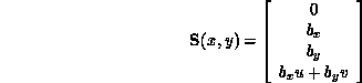
Here  is the fluid mass density,
E
is the specific energy,
u
and
v
are the fluid velocities in the
x
and
y
directions,
is the fluid mass density,
E
is the specific energy,
u
and
v
are the fluid velocities in the
x
and
y
directions,  and
and  are body force components, and the pressure,
p
, is given by,
are body force components, and the pressure,
p
, is given by,

where  is the constant adiabatic index. The motion of the fluid
is tracked by introducing massless marker particles and allowing them to be
advected with the flow. Thus, the number density of the marker particles,
is the constant adiabatic index. The motion of the fluid
is tracked by introducing massless marker particles and allowing them to be
advected with the flow. Thus, the number density of the marker particles,
 , satisfies,

The equations are solved on a rectilinear two-dimensional grid.
Second-order accuracy in time is maintained by first advancing the velocities
by a half time step, and then using these velocities to update all values
for the full time step. The size of the time step is governed by the
Courant condition.
The basic procedure in each time step is to first apply a five-point
difference operator at each grid point to convectively transport the field
values. These field values are then diffused in each of the positive and
negative
x
and
y
directions. The behavior of the resulting fields in the
vicinity of each grid point is then examined to determine how much diffusion
to remove at that point. In regions where a field value is locally
monotonic, nearly all the diffusion previously applied is removed for that
field. However, in regions close to extrema, the amount of diffusion removed
is less.
Guy Robinson
Wed Mar 1 10:19:35 EST 1995
6.2.3 Parallel Issues
Next:
6.2.4 Example Problem
Up:
Convectively-Dominated Flows and
Previous:
6.2.2 Mathematics and the
The code used in this study parallelizes well for a number of reasons. The
discretization is static and regular, and the same operations are applied at
each grid point, even though the evolution of the system is nonlinear. Thus,
the problem can be statically load balanced
at the
start of the code by ensuring that each processor's rectangular
subdomain contains the same number of grid points. In addition, the
physics, and hence the algorithm, is local so the finite difference
algorithm only requires communication between nearest neighbors in the
hypercube topology. The extreme regularity of the FCT technique means
that it can also be efficiently used to study convective transport on
SIMD concurrent computers, such as the Connection Machine,
as has been done by Oran, et al.
[
Oran:90a
].
No major changes were introduced into the sequential code in
parallelizing it for the hypercube architecture. Additional subroutines
were inserted to decompose the problem domain into rectangular
subdomains, and to perform interprocessor communication. Communication
is necessary in applying the Courant condition to determine the size of
the next time step, and in transferring field values at grid points
lying along the edge of a processor's subdomain. Single rows and
columns of field values were communicated as the algorithm required.
Some inefficiency, due to communication latency,
could
have been avoided if several rows and/or columns were communicated at
the same time, but in order to avoid wasting memory on larger
communication buffers, this was not done. This choice was dictated by
the small amount of memory (about  ) available on each
nCUBE-1
processor.
) available on each
nCUBE-1
processor.
Guy Robinson
Wed Mar 1 10:19:35 EST 1995
6.2.4 Example Problem
Next:
6.2.5 Performance and Results
Up:
Convectively-Dominated Flows and
Previous:
6.2.3 Parallel Issues
As a sample problem, the onset and growth of the Kelvin-Helmholtz
instability
was studied. This instability arises when the interface between two fluids
in shear motion is perturbed, and for this problem the body forces,  and
and
 , are zero. In Figure 6.2 (Color Plate), we show the development of the
Kelvin-Helmholtz instability at the interface of two fluids in shear motion.
In these figures, the density of the massless marker particles normalized by
the fluid density is plotted on a color map, with red corresponding to a
density of one through green, blue, and white to a density of zero. Initially,
all the marker particles are in the upper half of the domain, and the fluids
in the lower- and upper-half domains have a relative shear velocity in the
horizontal direction. An
, are zero. In Figure 6.2 (Color Plate), we show the development of the
Kelvin-Helmholtz instability at the interface of two fluids in shear motion.
In these figures, the density of the massless marker particles normalized by
the fluid density is plotted on a color map, with red corresponding to a
density of one through green, blue, and white to a density of zero. Initially,
all the marker particles are in the upper half of the domain, and the fluids
in the lower- and upper-half domains have a relative shear velocity in the
horizontal direction. An  finite difference
grid was used. Vortices form along the interface and
interact before being lost to numerical diffusion. By processing the
output from the nCUBE-1, a videotape of the evolution of the
instability was produced. This sample problem demonstrates that
the FCT technique is able to track the physical instability without
introducing numerical instability.
finite difference
grid was used. Vortices form along the interface and
interact before being lost to numerical diffusion. By processing the
output from the nCUBE-1, a videotape of the evolution of the
instability was produced. This sample problem demonstrates that
the FCT technique is able to track the physical instability without
introducing numerical instability.
Figure 6.2:
Development of the Kelvin-Helmholtz
instability at the interface of two fluids in shear motion.
Guy Robinson
Wed Mar 1 10:19:35 EST 1995
6.2.5 Performance and Results
Next:
6.2.6 Summary
Up:
Convectively-Dominated Flows and
Previous:
6.2.4 Example Problem

Table 6.1:
Timing Results in Seconds for a 512-processor and a
1-processor nCUBE-1. The values  and
and  represent the numbers
of grid points per processor in the
x
and
y
directions. The
concurrent efficiency, overhead, and speedup are denoted by
represent the numbers
of grid points per processor in the
x
and
y
directions. The
concurrent efficiency, overhead, and speedup are denoted by  ,
f
, and
S
.
,
f
, and
S
.
The code was timed for the Kelvin-Helmholtz problem for hypercubes with
dimension ranging from zero to nine. The results for the 512-processor case
are presented in Table
6.1
, and show a speedup of 429 for the
largest problem size considered. Subsequently, a group at Sandia National
Laboratories, using a modified version of the code, attained a speedup of
1009 on a 1024-processor nCUBE-1
for a similar type of problem
[
Gustafson:88a
]. The definitions of concurrent speedup, overhead, and
efficiency are given in Section
3.5
.
An analytic model of the performance of the concurrent algorithm was
developed, and ignoring communication latency, the concurrent overhead was
found to be proportional to  , where
n
is the number of grid
points per processor. This is in approximate agreement with the results
plotted in Figure
6.3
, that shows the concurrent overhead for a
number of different hypercubes dimensions and grain sizes.
, where
n
is the number of grid
points per processor. This is in approximate agreement with the results
plotted in Figure
6.3
, that shows the concurrent overhead for a
number of different hypercubes dimensions and grain sizes.
Guy Robinson
Wed Mar 1 10:19:35 EST 1995
6.2.6 Summary
Next:
Magnetism in the
Up:
Convectively-Dominated Flows and
Previous:
6.2.5 Performance and Results
The FCT
code was ported to the nCUBE-1 by David W. Walker
[
Walker:88b
]. Gary Montry of Sandia National Laboratories
supplied the original code, and made several helpful suggestions. A
videotape of the evolution of the Kelvin-Helmholtz instability was
produced by Jeff Goldsmith at the Image Processing
Laboratory of the Jet Propulsion Laboratory.
Figure 6.3:
Overhead,
f
, as a Function of  , Where
n
Is
the Number of Grid Points per Processor. Results are shown for nCUBE-1
hypercubes of dimension one to nine. The overhead for the 2-processor case
(open circles) lies below that for the higher dimensional hypercubes. This
is because the processors only communicate in one direction in the
2-processor case, whereas for hypercubes of dimension greater than one,
communication is necessary in both the
x
and
y
directions.
, Where
n
Is
the Number of Grid Points per Processor. Results are shown for nCUBE-1
hypercubes of dimension one to nine. The overhead for the 2-processor case
(open circles) lies below that for the higher dimensional hypercubes. This
is because the processors only communicate in one direction in the
2-processor case, whereas for hypercubes of dimension greater than one,
communication is necessary in both the
x
and
y
directions.
Guy Robinson
Wed Mar 1 10:19:35 EST 1995
Magnetism in the High-TemperatureSuperconductor Materials
Next:
6.3.1 Introduction
Up:
6 Synchronous Applications II
Previous:
6.2.6 Summary
Other References
HPFA Applications and Paradigms
Guy Robinson
Wed Mar 1 10:19:35 EST 1995
6.3.1 Introduction
Next:
6.3.2 The Computational Algorithm
Up:
Magnetism in the
Previous:
Magnetism in the
Following the discovery of high-temperature
superconductivity,
two-dimensional quantum
antiferromagnetic spin systems have received enormous attention from
physicists worldwide. It is generally believed that high-temperature
superconductivity occurs in the  planes, which is shown in
Figure
6.4
. Many features can be explained [
Anderson:87a
] in
the Hubbard theory of the strongly coupled electron, which at half-filling is
reduced to spin-1/2 antiferromagnetic Heisenberg
model:
planes, which is shown in
Figure
6.4
. Many features can be explained [
Anderson:87a
] in
the Hubbard theory of the strongly coupled electron, which at half-filling is
reduced to spin-1/2 antiferromagnetic Heisenberg
model:

where  are quantum spin
operators. Furthermore, the
neutron scattering experiments on the parent compound,
are quantum spin
operators. Furthermore, the
neutron scattering experiments on the parent compound,  ,
reveal a rich magnetic structure which is also modelled by this theory.
,
reveal a rich magnetic structure which is also modelled by this theory.
Physics in two dimensions (as compared to three dimensions) is characterized
by the large fluctuations. Many analytical methods work well in three
dimensions, but fail in two dimensions. For the quantum systems, this means
additional difficulties in finding solutions to the problem.
Figure 6.4:
The Copper-Oxygen Plane, Where the Superconductivity Is
Generally Believed to Occur. The arrows denote the quantum spins.
 ,
,  ,
,  denote the wave functions which
lead to the interactions among them.
denote the wave functions which
lead to the interactions among them.
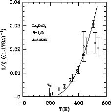
Figure:
Inverse Correlation Length of  Measured in Neutron
Scattering Experiment, Denoted by Cross; and Those Measured in our
Simulation, Denoted by Squares (Units in
Measured in Neutron
Scattering Experiment, Denoted by Cross; and Those Measured in our
Simulation, Denoted by Squares (Units in  .
.
 . At
. At  ,
,  undergoes a structural transition. The curve is the fit shown in
Figure
6.11
.
undergoes a structural transition. The curve is the fit shown in
Figure
6.11
.
New analytical methods have been developed to understand the low-T behavior
of these two-dimensional systems, and progress had been made. These methods
are essentially based on a  expansion. Unfortunately, the extreme
quantum case
expansion. Unfortunately, the extreme
quantum case  lies in the least reliable region of these
methods. On the other hand, given sufficient computer power, Quantum Monte
Carlo
simulation [
Ding:90g
] can provide
accurate numerical solutions of the model theory and quantitative comparison
with the experiment (see Figure
6.5
). Thus, simulations become a
crucial tool in studying these problems. The work described here has made a
significant contribution to the understanding of high-
lies in the least reliable region of these
methods. On the other hand, given sufficient computer power, Quantum Monte
Carlo
simulation [
Ding:90g
] can provide
accurate numerical solutions of the model theory and quantitative comparison
with the experiment (see Figure
6.5
). Thus, simulations become a
crucial tool in studying these problems. The work described here has made a
significant contribution to the understanding of high- materials, and
has been well received by the science community [
Maddox:90a
].
materials, and
has been well received by the science community [
Maddox:90a
].
Next:
6.3.2 The Computational Algorithm
Up:
Magnetism in the
Previous:
Magnetism in the
Guy Robinson
Wed Mar 1 10:19:35 EST 1995
6.3.2 The Computational Algorithm
Next:
6.3.3 Parallel Implementation and
Up:
Magnetism in the
Previous:
6.3.1 Introduction
Using the Suzuki-Trotter transformation
, the two-dimensional quantum problem
is converted into three-dimensional classical Ising
spins
with complicated interactions. The partition function becomes a product of
transfer matrices for each four-spin interaction
with  . These four-spin squares go in the time direction
on the three-dimensional lattice. This transfer matrix serves as the
probability basis for a Monte Carlo
simulation. The
zero matrix elements are the consequence of the quantum conservation
law. To avoid generating trial configurations with zero probability,
thus wasting the CPU time since these trials will never be accepted,
one should have the conservation law built into the updating scheme.
Two types of local moves may locally change the spin configurations, as
shown in Figure
6.6
. A global move in the time direction
flips all the spins along this time line. This update changes the
magnetization. Another global move in spatial directions changes the
winding numbers.
. These four-spin squares go in the time direction
on the three-dimensional lattice. This transfer matrix serves as the
probability basis for a Monte Carlo
simulation. The
zero matrix elements are the consequence of the quantum conservation
law. To avoid generating trial configurations with zero probability,
thus wasting the CPU time since these trials will never be accepted,
one should have the conservation law built into the updating scheme.
Two types of local moves may locally change the spin configurations, as
shown in Figure
6.6
. A global move in the time direction
flips all the spins along this time line. This update changes the
magnetization. Another global move in spatial directions changes the
winding numbers.
Figure 6.6:
(a) A ``Time-Flip.'' The white  plaquette is a
non-interacting one. The eight plaquettes surrounding it are interacting
ones. (b) A ``Space-Flip.'' The white
plaquette is a
non-interacting one. The eight plaquettes surrounding it are interacting
ones. (b) A ``Space-Flip.'' The white  plaquette is a
non-interacting one lying in spatial dimensions. The four plaquettes
going in time direction are interacting ones.
plaquette is a
non-interacting one lying in spatial dimensions. The four plaquettes
going in time direction are interacting ones.
This classical spin system in three dimensions is simulated using the
Metropolis
Monte Carlo algorithm. Starting with a
given initial configuration, we locate a closed loop
C
of
L
spins,
in one of the four moves. After checking that they satisfy the
conservation law, we compute  , the probability before all
L
spins are flipped, which is a product of the diagonal elements of the
transfer matrix; and
, the probability before all
L
spins are flipped, which is a product of the diagonal elements of the
transfer matrix; and  , the probability after the spins are
flipped, which is a product of the off-diagonal elements of the
transfer matrix along the loop
C
. The Metropolis procedure is to
accept the flip according to the probability
, the probability after the spins are
flipped, which is a product of the off-diagonal elements of the
transfer matrix along the loop
C
. The Metropolis procedure is to
accept the flip according to the probability  .
.
Figure 6.7:
A Vectorization of Eight ``Time-Flips.'' Spins along the
t
-direction are packed into computer words. The two 32-bit words,
S1 and S2, contain eight ``time plaquettes,'' indicated by the dashed
lines.
We implemented a simple and efficient multispin coding method which
facilitates vectorization and saves index calculation and memory
space. This is possible because each spin only has two states, up (1)
or down (0), which is represented by a single bit in a 32-bit integer.
Spins along the
t
-direction are packed into 32-bit words, so that
the boundary communication along the
x
or
y
direction can be
handled more easily. All the necessary checks and updates can be
handled by the bitwise logical operations OR, AND, NOT, and XOR.
Note that this is a natural vectorization, since AND operations for the
32 spins are carried out in the single AND operation by the CPU. The
index calculations to address these individual spins are also
minimized, because one only computes the index once for the 32 spins.
The same principles are applied for both local and global moves.
Figure
6.7
shows the case for time-loop coding.
Next:
6.3.3 Parallel Implementation and
Up:
Magnetism in the
Previous:
6.3.1 Introduction
Guy Robinson
Wed Mar 1 10:19:35 EST 1995
6.3.3 Parallel Implementation and Performance
Next:
6.3.4 Physics Results
Up:
Magnetism in the
Previous:
6.3.2 The Computational Algorithm
The fairly large three-dimensional lattices (usually  ) are partitioned into a ring of
M
processors with
x
-dimension which is uniformly distributed among the
M
processors.
The local updates are easily parallelized since the connection is, at
most, next-nearest neighbor (for the time-loop update). The needed
spin-word arrays from its neighbor are copied into the local storage by
the
shift
routine in the CrOS communication system
[
Fox:88a
] before doing the update. One of the global updates, the
time line, can also be done in the same fashion. The communication is
very efficient in the sense that a single communication shift,
) are partitioned into a ring of
M
processors with
x
-dimension which is uniformly distributed among the
M
processors.
The local updates are easily parallelized since the connection is, at
most, next-nearest neighbor (for the time-loop update). The needed
spin-word arrays from its neighbor are copied into the local storage by
the
shift
routine in the CrOS communication system
[
Fox:88a
] before doing the update. One of the global updates, the
time line, can also be done in the same fashion. The communication is
very efficient in the sense that a single communication shift,
 , spins instead of
Nt
spins in the case where the
lattice is partitioned into a two-dimensional grid. The
overhead/latency associated with the communication is thus
significantly reduced.
, spins instead of
Nt
spins in the case where the
lattice is partitioned into a two-dimensional grid. The
overhead/latency associated with the communication is thus
significantly reduced.
The winding-line global update along the
x
-direction is difficult to do in
this fashion, because it involves spins on all the
M
nodes. In addition,
we need to compute the correlation functions which have the same difficulty.
However, since these operations are not used very often, we devised a fairly
elegant way to parallelize these global operations. A set of
gather-scatter
routines, based on the
cread
and
cwrite
in
CrOS, is written. In
gather
, the subspaces on each node are gathered
into complete spaces on each node, preserving the original geometric
connection. Parallelism is achieved now since the global operations are done
on each node just as in the sequential computer, with each node only doing
the part it originally covers. In
scatter
, the updated (changed)
lattice configuration on a particular node (number zero) is scattered
(distributed) back to all the nodes in the ring, exactly according to the
original partition. Note that this scheme differs from the earlier
decomposition scheme [
Fox:84a
] for the gravitation problem, where memory
size constraint is the main concern.
The hypercube nodes were divided into several
independent
rings,
each ring holding an independent simulation, as shown in
Figure
6.8
. At higher temperatures, a spin system of
 is enough, so that we can simulate several independent systems
at the same time. At low temperatures, one needs larger systems, such as
is enough, so that we can simulate several independent systems
at the same time. At low temperatures, one needs larger systems, such as
 -all the nodes will then be dedicated to a single large
system. This simple parallelism makes the simulation very flexible and
efficient. In the simulation, we used a parallel version of the Fibonacci
additive random numbers
generator [
Ding:88d
],
which has a period larger that
-all the nodes will then be dedicated to a single large
system. This simple parallelism makes the simulation very flexible and
efficient. In the simulation, we used a parallel version of the Fibonacci
additive random numbers
generator [
Ding:88d
],
which has a period larger that  .
.
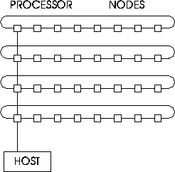
Figure 6.8:
The Configuration of the Hypercube Nodes. In the example, 32
nodes are configured as four independent rings, each consisting of 8
nodes. Each ring does an independent simulation.
We have made a systematic performance analysis
by running the code on
different sizes and different numbers of nodes. The timing results
for a realistic situation (20 sweeps of update, one measurement) are measured
[
Ding:90k
]. The speedup,  /
/ , where
  (
( ) is the
time for the same size spins system to run same number operations on one
) is the
time for the same size spins system to run same number operations on one
 node, is plotted in Figure
6.9
. One can see that speedup
is quite close to the ideal case, denoted by the dashed line. For the
node, is plotted in Figure
6.9
. One can see that speedup
is quite close to the ideal case, denoted by the dashed line. For the
 quantum spin system, the 32-node hypercube speeds up
the computation by a factor of 26.6, which is a very good result. However,
running the same spin system on a 16-node is more efficient, because we can
run two independent systems on the 32-node hypercube with a total speedup
of
quantum spin system, the 32-node hypercube speeds up
the computation by a factor of 26.6, which is a very good result. However,
running the same spin system on a 16-node is more efficient, because we can
run two independent systems on the 32-node hypercube with a total speedup
of  (each speedup a factor 14.5). This is better described
by
efficiency
, defined as speedup/nodes, which is plotted in
Figure
6.10
. Clearly, the efficiency of the implementation is very
high, generally over 90%.
(each speedup a factor 14.5). This is better described
by
efficiency
, defined as speedup/nodes, which is plotted in
Figure
6.10
. Clearly, the efficiency of the implementation is very
high, generally over 90%.
Figure 6.9:
Speedup of the Parallel Algorithm for Lattice Systems  ,
,  and
and  . The dashed line is the ideal
case.
. The dashed line is the ideal
case.
Figure 6.10:
Efficiency of the Parallel Algorithm
Comparison with other supercomputers is interesting. For this
program, the one-head CRAY X-MP
speed is
approximately that of a 2-node Mark IIIfp. This indicates that our
32-node Mark IIIfp
performs better than the
CRAY X-MP by about a factor of  % = 14! We note that
our code is written in C and the vectorization is limited to the 32-bit
inside the words. Rewriting the code in Fortran (Fortran compilers on
the CRAY are more efficient) and fully vectorizing the code, one may
gain a factor of about three on the CRAY. Nevertheless, this quantum
Monte Carlo code is clearly a good example, in that parallel computers
easily (i.e., at same programming level) outperform the conventional
supercomputers.
% = 14! We note that
our code is written in C and the vectorization is limited to the 32-bit
inside the words. Rewriting the code in Fortran (Fortran compilers on
the CRAY are more efficient) and fully vectorizing the code, one may
gain a factor of about three on the CRAY. Nevertheless, this quantum
Monte Carlo code is clearly a good example, in that parallel computers
easily (i.e., at same programming level) outperform the conventional
supercomputers.
Next:
6.3.4 Physics Results
Up:
Magnetism in the
Previous:
6.3.2 The Computational Algorithm
Guy Robinson
Wed Mar 1 10:19:35 EST 1995
6.3.4 Physics Results
Next:
6.3.5 Conclusions
Up:
Magnetism in the
Previous:
6.3.3 Parallel Implementation and
We obtained many good results which were previously unknown. Among them, the
correlation functions are perhaps the most important. First, the results can
be directly compared with experiments, thus providing new understanding of
the magnetic structure of the high-temperature superconducting materials.
Second, and no less important, is the behavior of the correlation function we
obtained which gives a crucial test of the assessment of various approximate
methods.
In the large spin-
S
(classical) system, the correlation
length
goes as

at low temperatures. This predicts a too-large correlation length, compared
with experimental results. As  , the quantum
fluctuations in the system become significant. Several approximate
methods [
Chakravarty:88a
], [
Auerbach:88a
] predict a similar low-
T
behavior.
, the quantum
fluctuations in the system become significant. Several approximate
methods [
Chakravarty:88a
], [
Auerbach:88a
] predict a similar low-
T
behavior.  ,
,  , and
p=0
or
1
.
, and
p=0
or
1
.  is a quantum
renormalization constant.
is a quantum
renormalization constant.
Our extensive quantum Monte Carlo simulations were performed [
Ding:90g
]
on the spin- system as large as
  at low
temperature range
at low
temperature range  -1.0. The correlation length, as a
function of
-1.0. The correlation length, as a
function of  , is plotted in Figure
6.11
. The data points fall
onto a straight line, surprisingly well, throughout the whole temperature
range, leading naturally to the pure exponential form:
, is plotted in Figure
6.11
. The data points fall
onto a straight line, surprisingly well, throughout the whole temperature
range, leading naturally to the pure exponential form:

where
a
is the lattice constant. This provides a crucial support to the
above-mentioned theories. Quantitatively,

or

Figure 6.11:
Correlation Length Measured at Various Temperatures. The
straight line is the fit.
Direct comparison with experiments will not only test the validity of
the Heisenberg model, but also determine the important parameter, the
exchange coupling
J
. The spacing between
Cu
atoms in  plane
is
plane
is  . Setting
  , the Monte
Carlo data is compared with those from neutron scattering experiments
[
Endoh:88a
] in Figure
6.5
. The agreement is very
good. This provides strong evidence that the essential magnetic
behavior is captured by the Heisenberg model.
The quantum Monte Carlo
result is an accurate first
principle calculation; no adjustable parameter is involved. Comparing
directly with the experiment, the only adjustable parameter is
J
.
This gives an independent determination of the
effective
exchange
coupling:
, the Monte
Carlo data is compared with those from neutron scattering experiments
[
Endoh:88a
] in Figure
6.5
. The agreement is very
good. This provides strong evidence that the essential magnetic
behavior is captured by the Heisenberg model.
The quantum Monte Carlo
result is an accurate first
principle calculation; no adjustable parameter is involved. Comparing
directly with the experiment, the only adjustable parameter is
J
.
This gives an independent determination of the
effective
exchange
coupling:

Note that near  , the experimentally measured
correlation is systematically smaller than the theoretical curve, shown in
Equation
6.4
. This is a combined result of small effects:
frustration, anisotropies, inter-layer coupling, and so on.
, the experimentally measured
correlation is systematically smaller than the theoretical curve, shown in
Equation
6.4
. This is a combined result of small effects:
frustration, anisotropies, inter-layer coupling, and so on.
Various moments of the Raman spectrum are calculated using series expansions
and comparing with experiments [
Singh:89a
]. This gives an estimate,
 (
( ), which is quite
close to the above value determined from correlation functions. Raman
scattering probes the short wavelength region, whereas neutron scattering
measures the long-range correlations. The agreement of
J
's obtained from
these two rather different experiments is another significant indication that
the magnetic interactions are dominated by the Heisenberg model.
), which is quite
close to the above value determined from correlation functions. Raman
scattering probes the short wavelength region, whereas neutron scattering
measures the long-range correlations. The agreement of
J
's obtained from
these two rather different experiments is another significant indication that
the magnetic interactions are dominated by the Heisenberg model.
Equation
6.4
is valid for all the quantum AFM spins. The classic
two-dimensional antiferromagnetic system discovered twenty years ago
[
Birgeneau:71a
],  , is a spin-one system with
 . Very recently, Birgeneau [
Birgeneau:90a
] fitted the
measured correlation lengths to
. Very recently, Birgeneau [
Birgeneau:90a
] fitted the
measured correlation lengths to

The fit is very good, as shown in Figure
6.12
. The factor
( ) comes from integration of the two-loop
  -function without
taking the
-function without
taking the  limit, and could be neglected if
T
is very
close to 0. For the spin-
limit, and could be neglected if
T
is very
close to 0. For the spin- AFM
AFM  ,
Equation
6.4
also describes the data quite well [
Higgins:88a
].
,
Equation
6.4
also describes the data quite well [
Higgins:88a
].
Figure 6.12:
Correlation Length of  Measured in Neutron
Scattering Experiment with the Fit.
Measured in Neutron
Scattering Experiment with the Fit.
A common feature from Figures
6.11
and
6.12
is that
the scaling equation Equation
6.4
, which is derived near  ,
is valid for a wide range of
T
, up to
,
is valid for a wide range of
T
, up to  . This differs
drastically from the range of criticality in three-dimensional systems, where
the width
. This differs
drastically from the range of criticality in three-dimensional systems, where
the width  is usually about 0.2 or less. This is a
consequence of the crossover temperature
is usually about 0.2 or less. This is a
consequence of the crossover temperature  [
Chakravarty:88a
],
where the Josephson length scale becomes compatible with the thermal wave
length, being relatively high,
[
Chakravarty:88a
],
where the Josephson length scale becomes compatible with the thermal wave
length, being relatively high,  . This property is a general
character in the low critical dimensions. In the quantum XY model, a
Kosterlitz-Thouless transition
occurs
[
Ding:90b
] at
. This property is a general
character in the low critical dimensions. In the quantum XY model, a
Kosterlitz-Thouless transition
occurs
[
Ding:90b
] at  and the critical behavior remains valid up
to
and the critical behavior remains valid up
to  .
.
As emphasized by Birgeneau, the spin-wave value

S=1
,  , fits the experiment quite well, whereas for
 , spin-wave value
  differs significantly from the
correct value 1.25 as in Equation
6.4
. This indicates that the
large quantum fluctuations in the spin-
differs significantly from the
correct value 1.25 as in Equation
6.4
. This indicates that the
large quantum fluctuations in the spin- system are not
adequately accounted for in the spin-wave theory, whereas for the spin-one
system, they are.
system are not
adequately accounted for in the spin-wave theory, whereas for the spin-one
system, they are.
Figure
6.13
shows the energy density at various temperatures. At
higher
T
, the high-temperature series expansion accurately reproduces our
data. At low
T
,
E
approaches a finite ground state energy. Another
useful thermodynamical quantity is uniform susceptibility, which is shown in
Figure
6.14
. Again, at high-
T
, series expansion coincides with
our data. The maximum point occurs at  with
with
 . This is useful in determining
J
and
. This is useful in determining
J
and
 for the material.
Figure 6.13:
Energy Measured as a Function of Temperature. Squares are from
our work. The curve is the 10th order high-T expansion.
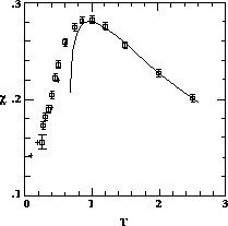
Figure:
Uniform Susceptibility Measured as a Function of Temperature.
Symbols are similar to Figure
6.13
.
Next:
6.3.5 Conclusions
Up:
Magnetism in the
Previous:
6.3.3 Parallel Implementation and
Guy Robinson
Wed Mar 1 10:19:35 EST 1995
6.3.5 Conclusions
Next:
Phase Transitions in
Up:
Magnetism in the
Previous:
6.3.4 Physics Results
In conclusion, the quantum AFM Heisenberg spins are now well understood
theoretically. The data from neutron scattering experiments for both
 ,
,  and
S=1
,
and
S=1
,  compare quite well.
For
compare quite well.
For  , this leads to a direct determination
  .
.
Quantum spins are well suited for the hypercube computer. Its spatial
decomposition is straightforward; the short-range nature (excluding the
occasional long-range one) of interaction makes the extension to large
numbers of processors simple. Hypercube connections made the use of the node
computer efficient and flexible. High speedup can be achieved with
reasonable ease, provided one improves the algorithm to minimize the
communications.
The work described here is the result of the collaboration between
H. Q. Ding and M. S. Makivic.
Guy Robinson
Wed Mar 1 10:19:35 EST 1995
Phase Transitions in Two-dimensionalQuantum Spin Systems
Next:
6.4.1 The case of
Up:
6 Synchronous Applications II
Previous:
6.3.5 Conclusions
In this section, we discuss two further important developments based on the
previous section (Section
6.3
) on the isotropic Heisenberg quantum
spins. These extensions are important in treating the observed phase
transitions
in the two-dimensional magnetic systems. Theoretically, two-dimensional
isotropic Heisenberg quantum spins
remain in paramagnetic
state at all
temperatures [
Mermin:66a
]. However, all crystals found in nature with
strong two-dimensional magnetic characters go through phase transitions into
ordered states [
Birgeneau:71a
], [
DeJongh:74a
]. These include the
recently discovered high- materials,
  and
and
 , despite the presence of large quantum fluctuations in
the spin-
, despite the presence of large quantum fluctuations in
the spin- antiferromagnets.
We consider the cases where the magnetic spins interact through

In the case  , the system goes through an Ising-like
antiferromagnetic transition, very similar to those that occur in the
high-
, the system goes through an Ising-like
antiferromagnetic transition, very similar to those that occur in the
high- materials. In the case
h = -J
, that is, the XY model, the
system exhibits a Kosterlitz-Thouless type of transition. In both cases, our
simulation provides convincing and complete results for the first time.
materials. In the case
h = -J
, that is, the XY model, the
system exhibits a Kosterlitz-Thouless type of transition. In both cases, our
simulation provides convincing and complete results for the first time.
Through the Matsubara-Matsuda transformation between spin-1/2 operator
 and bosonic creation/destruction operations
  and
and  ,
a general quantum system can be mapped into quantum spin
system. Therefore, the phase transitions described here apply to
general two-dimensional quantum systems. These results have broad
implications in two-dimensional physical systems in particular, and the
statistical systems in general.
,
a general quantum system can be mapped into quantum spin
system. Therefore, the phase transitions described here apply to
general two-dimensional quantum systems. These results have broad
implications in two-dimensional physical systems in particular, and the
statistical systems in general.
Other References
HPFA Applications and Paradigms
Guy Robinson
Wed Mar 1 10:19:35 EST 1995
6.4.1 The case of : Antiferromagnetic Transitions
Next:
Origin of the
Up:
Phase Transitions in
Previous:
Phase Transitions in
The popular explanation for the antiferromagnetic ordering transitions in
these high- materials emphasizes the very small coupling,
  , between
the two-dimensional layers,
, between
the two-dimensional layers,  , and is estimated to be about
  .
However, all these systems exhibit some kind of in-plane anisotropies, which
is of order
.
However, all these systems exhibit some kind of in-plane anisotropies, which
is of order  . An interesting case is the spin-one crystal,
 , discovered twenty years ago [
Birgeneau:71a
]. The
magnetic behavior of
, discovered twenty years ago [
Birgeneau:71a
]. The
magnetic behavior of  exhibits very strong two-dimensional
characters with an exchange coupling
exhibits very strong two-dimensional
characters with an exchange coupling  . It has a Néel
ordering transition at
. It has a Néel
ordering transition at  , induced by an Ising-like anisotropy,
 .
.
Our simulation provides clear evidence to support the picture that the
in-plane anisotropy is also quite important in bringing about the observed
antiferromagnetic transition at the most interesting spin- case.
Adding an anisotropy energy as small as
case.
Adding an anisotropy energy as small as  will induce an ordering
transition at
will induce an ordering
transition at  . This striking effect and related results
agree well with a wide class of experiments, and provide some insights
into these types of materials.
. This striking effect and related results
agree well with a wide class of experiments, and provide some insights
into these types of materials.
Guy Robinson
Wed Mar 1 10:19:35 EST 1995
Origin of the Interaction
Next:
Simulation Results
Up:
6.4.1 The case of
Previous:
6.4.1 The case of
In the antiferromagnetic spin system, superexchange leads to the dominant
isotropic coupling. One of the high-order effects, due to
crystal field, is written as  , which is a constant for these
spin-
, which is a constant for these
spin- high-
high- materials. Another second-order effect is the
spin-orbital coupling. This effect will pick up a preferred direction and
lead to an
materials. Another second-order effect is the
spin-orbital coupling. This effect will pick up a preferred direction and
lead to an  term, which also arises due to the lattice distortion
in
term, which also arises due to the lattice distortion
in  . More complicated terms, like the antisymmetric exchange,
can also be generated. For simplicity and clarity, we focus the study on the
antiferromagnetic Heisenberg model with an Ising-like anisotropy as in
Equation
6.12
. The anisotropy parameter
h
relates to the usual
reduced anisotropy energy
. More complicated terms, like the antisymmetric exchange,
can also be generated. For simplicity and clarity, we focus the study on the
antiferromagnetic Heisenberg model with an Ising-like anisotropy as in
Equation
6.12
. The anisotropy parameter
h
relates to the usual
reduced anisotropy energy  through
  . In the past, the
anisotropy field model,
. In the past, the
anisotropy field model,  , has also been
included. However, its origin is less clear and, furthermore, the
Ising symmetry is explicitly broken.
, has also been
included. However, its origin is less clear and, furthermore, the
Ising symmetry is explicitly broken.
Guy Robinson
Wed Mar 1 10:19:35 EST 1995
Simulation Results
Next:
Theoretical Interpretation
Up:
6.4.1 The case of
Previous:
Origin of the
For the large anisotropy system,
h=1
, the specific heat  are shown for
several spin systems in Figure
6.15
(a). The peak becomes sharper
and higher as the system size increases, indicating a divergent peak in an
infinite system, similar to the two-dimensional Ising model. Defining the
transition temperature
are shown for
several spin systems in Figure
6.15
(a). The peak becomes sharper
and higher as the system size increases, indicating a divergent peak in an
infinite system, similar to the two-dimensional Ising model. Defining the
transition temperature  at the peak of
  for the finite
 system, the finite-size scaling theory [
Landau:76a
] predicts
that
system, the finite-size scaling theory [
Landau:76a
] predicts
that  relates to
  through the scaling law

Setting  , the Ising exponent, a good fit with
  , is
shown in Figure
6.15
(b). A different scaling with the same
exponent for the correlation length,
, is
shown in Figure
6.15
(b). A different scaling with the same
exponent for the correlation length,

is also satisfied quite well, resulting in  . The
staggered magnetization drops down near
. The
staggered magnetization drops down near  , although the behaviors are
rounded off on these finite-size systems. All the evidence clearly
indicates that an Ising-like antiferromagnetic transition occurs at
, although the behaviors are
rounded off on these finite-size systems. All the evidence clearly
indicates that an Ising-like antiferromagnetic transition occurs at  , with a divergent specific heat. In the smaller anisotropy case,
 , similar behaviors are found. The scaling for the correlation length
is shown in Figure
6.16
, indicating a transition at
, similar behaviors are found. The scaling for the correlation length
is shown in Figure
6.16
, indicating a transition at  .
However, the specific heat remains finite at all temperatures.
.
However, the specific heat remains finite at all temperatures.
Figure 6.15:
(a) The Specific Heat for Different Size Systems of
h=1
. (b)
Finite Size Scaling for  .
.
Figure 6.16:
The Inverse Correlation Lengths for  System
(
System
( ),
),  System (
 ), and
h=0
System
(
), and
h=0
System
( ) for the Purpose of Comparison. The straight lines are the
scaling relation:
) for the Purpose of Comparison. The straight lines are the
scaling relation:  . From it we can pin down
 .
.
The most interesting case is  (or
(or  , very close to those
in
, very close to those
in  [
Birgeneau:71a
]). Figure
6.17
shows the
staggered correlation function at
[
Birgeneau:71a
]). Figure
6.17
shows the
staggered correlation function at  compared with those on the
isotropic model [
Ding:90g
]. The inverse correlation length measured,
together with those for the isotropic model (
h=0
), are shown in
Figure
6.16
. Below
compared with those on the
isotropic model [
Ding:90g
]. The inverse correlation length measured,
together with those for the isotropic model (
h=0
), are shown in
Figure
6.16
. Below  , the Ising behavior of
a straight line becomes clear. Clearly, the system becomes
antiferromagnetically ordered around
, the Ising behavior of
a straight line becomes clear. Clearly, the system becomes
antiferromagnetically ordered around  . The best estimate is

Figure 6.17:
The Correlation Function on the  System at
  for
for  system. It decays with correlation length
  . Also shown is the isotropic case
h=0
, which has
. Also shown is the isotropic case
h=0
, which has  .
.
Next:
Theoretical Interpretation
Up:
6.4.1 The case of
Previous:
Origin of the
Guy Robinson
Wed Mar 1 10:19:35 EST 1995
Theoretical Interpretation
Next:
Comparison with Experiments
Up:
6.4.1 The case of
Previous:
Simulation Results
It may seem a little surprising that a very small anisotropy can lead to a
substantially high  . This may be explained by the following argument.
At low
T
, the spins are highly correlated in the isotropic case. Since no
direction is preferred, the correlated spins fluctuate in all directions,
resulting in zero net magnetization. Adding a very small anisotropy into the
system introduces a preferred direction, so that the already highly
correlated spins will fluctuate around this direction, leading to a global
magnetization.
. This may be explained by the following argument.
At low
T
, the spins are highly correlated in the isotropic case. Since no
direction is preferred, the correlated spins fluctuate in all directions,
resulting in zero net magnetization. Adding a very small anisotropy into the
system introduces a preferred direction, so that the already highly
correlated spins will fluctuate around this direction, leading to a global
magnetization.
More quantitatively, the crossover from the isotropic Heisenberg behavior to
the Ising behavior occurs at  , where the correlation length is of
order of some power of the inverse anisotropy. From the scaling
arguments [
Riedel:69a
],
, where the correlation length is of
order of some power of the inverse anisotropy. From the scaling
arguments [
Riedel:69a
],  where
where  is the crossover exponent. In the two-dimensional model, both
 and
and  are infinite, but the ratio is approximately 1/2. For
 , this relation indicates that the Ising behavior is valid for
 , which is clearly observed in Figure
6.16
.
Similar crossover around
, which is clearly observed in Figure
6.16
.
Similar crossover around  for
for  is also
observed in Figure
6.16
. At low
T
, for the isotropic quantum
model, the correlation length behaves as [
Ding:90g
]
is also
observed in Figure
6.16
. At low
T
, for the isotropic quantum
model, the correlation length behaves as [
Ding:90g
]
 where
where  . Therefore,
we expect
. Therefore,
we expect

where  is spin-
S
dependent constant of order one.
Therefore, even a very small anisotropy
is spin-
S
dependent constant of order one.
Therefore, even a very small anisotropy  will induce a phase
transition
at a substantially high temperature
(
will induce a phase
transition
at a substantially high temperature
( ). This crude picture, suggested a long time ago to
explain the observed phase transitions, is now confirmed by the
extensive quantum Monte Carlo
simulations for the
first time. Note that this problem is an extreme case both because it
is an antiferromagnet (more difficult to become ordered than the
ferromagnet), and because it has the largest quantum fluctuations
(spin-
). This crude picture, suggested a long time ago to
explain the observed phase transitions, is now confirmed by the
extensive quantum Monte Carlo
simulations for the
first time. Note that this problem is an extreme case both because it
is an antiferromagnet (more difficult to become ordered than the
ferromagnet), and because it has the largest quantum fluctuations
(spin- ). Since
  varies slowly with
h
, we can
estimate
varies slowly with
h
, we can
estimate  at
at  :
:

Next:
Comparison with Experiments
Up:
6.4.1 The case of
Previous:
Simulation Results
Guy Robinson
Wed Mar 1 10:19:35 EST 1995
Comparison with Experiments
Next:
The Case of
Up:
6.4.1 The case of
Previous:
Theoretical Interpretation
This simple result correctly predicts  for a wide class of
crystals found in nature, assuming the same level of anisotropy, that
is,
for a wide class of
crystals found in nature, assuming the same level of anisotropy, that
is,  . The high-
 superconductor
 exhibits a Néel
transition at
exhibits a Néel
transition at  . With
  , our results give quite a close estimate:
 . Similar close predictions hold for other
 systems, such as superconductor
  and
insulator
and
insulator  . For the high-
 material
  ,
,
 [
Ding:90g
]. This material undergoes a Néel
transition at
[
Ding:90g
]. This material undergoes a Néel
transition at  . Our prediction of
  is in the same range of
  , and much better than the
naive expectation that
, and much better than the
naive expectation that  . In this
crystal, there is some degree of frustration
(see
below), so the actual transition is pushed down. These examples
clearly indicate that the in-plane anisotropy could be quite important
to bring the system to the Néel order for these high-
. In this
crystal, there is some degree of frustration
(see
below), so the actual transition is pushed down. These examples
clearly indicate that the in-plane anisotropy could be quite important
to bring the system to the Néel order for these high- materials. For the
S=1
system,
materials. For the
S=1
system,  , our results predict a
 , quite close to the observed
  .
.
These results have direct consequences regarding the critical
exponents.
The onset of transition is
entirely due to the Ising-like anisotropy. Once the system becomes
Néel-ordered, different layers in the three-dimensional crystals will
order at the same time. Spin fluctuations, in different layers, are
incoherent so that the critical exponents such as  ,
,  ,
and
,
and  will be the two, rather than three-dimensional Ising
exponents.
will be the two, rather than three-dimensional Ising
exponents.  and
and  show such
behaviors clearly. However, the interlayer coupling, although very
small (much smaller than the in-plane anisotropy), could induce
coherent correlations between the layers, so that the critical
exponents will be somewhere between the two and three-dimensional Ising
exponents.
show such
behaviors clearly. However, the interlayer coupling, although very
small (much smaller than the in-plane anisotropy), could induce
coherent correlations between the layers, so that the critical
exponents will be somewhere between the two and three-dimensional Ising
exponents.  and
and  seem to belong to
this category.
seem to belong to
this category.
Whether the ground state of the spin- antiferromagnet spins has
the long-range Néel order, is a longstanding problem [
Anderson:87a
].
The existence of the Néel order is vigorously proved for
antiferromagnet spins has
the long-range Néel order, is a longstanding problem [
Anderson:87a
].
The existence of the Néel order is vigorously proved for  . In
the most interesting case
. In
the most interesting case  , numerical calculations on small lattices
suggested the existence of the long-range order. Our simulation establishes
the long-range order for
, numerical calculations on small lattices
suggested the existence of the long-range order. Our simulation establishes
the long-range order for  .
.
The fact that near  , the spin system is quite sensitive to the
tiny anisotropy could have a number of important consequences. For
example, the correlation lengths measured in
, the spin system is quite sensitive to the
tiny anisotropy could have a number of important consequences. For
example, the correlation lengths measured in  are
systematically smaller than the theoretical prediction [
Ding:90g
]
near
are
systematically smaller than the theoretical prediction [
Ding:90g
]
near  . The weaker correlations probably indicate that the
frustrations, due to the next to nearest neighbor interaction, come
into play. This is consistent with the fact that
. The weaker correlations probably indicate that the
frustrations, due to the next to nearest neighbor interaction, come
into play. This is consistent with the fact that  is below the
 suggested by our results.
Next:
The Case of
Up:
6.4.1 The case of
Previous:
Theoretical Interpretation
Guy Robinson
Wed Mar 1 10:19:35 EST 1995
The Case of : Quantum XY Model and
theTopological Transition
Next:
A Brief History
Up:
Phase Transitions in
Previous:
Comparison with Experiments
It is well known now that the two-dimensional (2D) classical (planar) XY
model
undergoes Kosterlitz-Thouless (KT)
[
Kosterlitz:73a
] transition at
 [
Gupta:88a
], characterized by exponentially divergent
correlation length and in-plane susceptibility. The transition, due to the
unbinding of vortex-antivortex pairs, is weak; the specific heat has a finite
peak above
[
Gupta:88a
], characterized by exponentially divergent
correlation length and in-plane susceptibility. The transition, due to the
unbinding of vortex-antivortex pairs, is weak; the specific heat has a finite
peak above  .
.
Does the two-dimensional quantum XY model
go
through a phase transition? If so, what type of transition? This is a
longstanding problem in statistical physics. The answers are relevant
to a wide class of two-dimensional problems such as magnetic
insulators, superfluidity, melting, and possibly to the recently
discovered high- superconducting transition. Physics in two
dimensions is characterized by large fluctuations. Changing from the
classical model to the quantum model, additional quantum fluctuations
(which are particularly strong in the case of spin-1/2) may alter the
physics significantly. A direct consequence is that the already weak
KT transition could be washed out completely.
superconducting transition. Physics in two
dimensions is characterized by large fluctuations. Changing from the
classical model to the quantum model, additional quantum fluctuations
(which are particularly strong in the case of spin-1/2) may alter the
physics significantly. A direct consequence is that the already weak
KT transition could be washed out completely.
Guy Robinson
Wed Mar 1 10:19:35 EST 1995
A Brief History
Next:
Evidence for the
Up:
The Case of
Previous:
The Case of
The quantum XY model
was first proposed
[
Matsubara:56a
] in 1956 to study the lattice quantum fluids.
Later, high-temperature series studies raised the possibility of a
divergent susceptibility for the two-dimensional model. For the
classical planar model, the remarkable theory of Kosterlitz and
Thouless [
Kosterlitz:73a
] provided a clear physical picture and
correctly predicted a number of important properties. However, much
less is known about the quantum model. In fact, it has been
controversial. Using a large-order high-temperature expansion,
Rogiers, et al. [
Rogiers:79a
] suggested a second-order
transition at  for spin-1/2. Later, real-space
renormalization group analysis was applied to the model with
contradictory and inconclusive results. DeRaedt, et al.
[
DeRaedt:84a
] then presented an exact solution and Monte Carlo
simulation, both based on the Suzuki-Trotter transformation with small
Trotter number
m
. Their results, both analytical and numerical,
supported an Ising-like (second-order) transition at the Ising
point
for spin-1/2. Later, real-space
renormalization group analysis was applied to the model with
contradictory and inconclusive results. DeRaedt, et al.
[
DeRaedt:84a
] then presented an exact solution and Monte Carlo
simulation, both based on the Suzuki-Trotter transformation with small
Trotter number
m
. Their results, both analytical and numerical,
supported an Ising-like (second-order) transition at the Ising
point  , with a logarithmically
divergent specific heat. Loh, et al. [
Loh:85a
] simulated
the system with an improved technique. They found that specific peak
remains finite and argued that a phase transition occurs at
, with a logarithmically
divergent specific heat. Loh, et al. [
Loh:85a
] simulated
the system with an improved technique. They found that specific peak
remains finite and argued that a phase transition occurs at
 -0.5 by measuring the change of the ``twist energy'' from the
 lattice to the
  lattice. The dispute between
DeRaedt, et al., and Loh, et al., centered on the
importance of using a large Trotter number
m
and the global updates
in small-size systems, which move the system from one subspace to
another. Recent attempts to solve this problem still add fuel to the
controversy.
lattice. The dispute between
DeRaedt, et al., and Loh, et al., centered on the
importance of using a large Trotter number
m
and the global updates
in small-size systems, which move the system from one subspace to
another. Recent attempts to solve this problem still add fuel to the
controversy.
Guy Robinson
Wed Mar 1 10:19:35 EST 1995
Evidence for the Transition
Next:
Implications
Up:
The Case of
Previous:
A Brief History
The key to pinning down the existence and type of transition is a study
of correlation length and in-plane susceptibility, because their
divergences constitute the most direct evidence of a phase transition.
These quantities are much more difficult to measure, and large lattices
are required in order to avoid finite size effects. These key points
are lacking in the previous works, and are the focus of our study. By
extensive use of the Mark IIIfp Hypercube, we are able to measure spin
correlations and thermodynamic quantities accurately on very large
lattices ( ). Our work
[Ding:90h;92a] provides convincing evidence that a phase transition
does occur at a finite temperature in the extreme quantum case, spin-
). Our work
[Ding:90h;92a] provides convincing evidence that a phase transition
does occur at a finite temperature in the extreme quantum case, spin- .
At transition point,
.
At transition point,  , the correlation length
and susceptibility diverge exactly according to the form of
Kosterlitz-Thouless (Equation
6.18
).
, the correlation length
and susceptibility diverge exactly according to the form of
Kosterlitz-Thouless (Equation
6.18
).
We plot the correlation length,  , and the susceptibility,
  , in
Figures
6.18
and
6.19
. They show a tendency of
divergence at some finite
, in
Figures
6.18
and
6.19
. They show a tendency of
divergence at some finite  . Indeed, we fit them to the form predicted
by Kosterlitz and Thouless for the classical model
. Indeed, we fit them to the form predicted
by Kosterlitz and Thouless for the classical model

The fit is indeed very good ( per degree of freedom is 0.81),
as shown in Figure
6.18
. The fit for correlation length gives
per degree of freedom is 0.81),
as shown in Figure
6.18
. The fit for correlation length gives

A similar fit for susceptibility,  is also very good
(
is also very good
( ):
):

as shown in Figure
6.19
. The good quality of both fits and the
closeness of  's obtained are the main results of this work. The fact
that these fits also reproduce the expected scaling behavior
's obtained are the main results of this work. The fact
that these fits also reproduce the expected scaling behavior  with
with

is a further consistency check. These results strongly indicate that the
spin-1/2 XY model undergoes a Kosterlitz-Thouless phase transition at
 . We note that this
  is consistent with the trend
of the ``twist energy'' [
Loh:85a
] and that the rapid increase of vortex
density near
is consistent with the trend
of the ``twist energy'' [
Loh:85a
] and that the rapid increase of vortex
density near  is due to the unbinding of vortex pairs.
Figures
6.18
and
6.19
also indicate that the
critical region
is due to the unbinding of vortex pairs.
Figures
6.18
and
6.19
also indicate that the
critical region  is quite wide (
 ), which is very similar
to the spin-1/2 Heisenberg model, where the
), which is very similar
to the spin-1/2 Heisenberg model, where the  behavior holds
up to
behavior holds
up to  . These two-dimensional phenomena are in sharp contrast to
the usual second-order transitions in three dimensions.
. These two-dimensional phenomena are in sharp contrast to
the usual second-order transitions in three dimensions.
Figure 6.18:
Correlation Length and Fit. (a)  versus
T
. The vertical
line indicates
versus
T
. The vertical
line indicates  diverges at
  ; (b)
; (b)  versus
 . The straight line indicates
  .
.
Figure:
(a) This figure repeats the plot of Figure
6.18
(a)
showing on a coarser scale both the high temperature expansion (HTE) and the
Kosterlitz-Thouless fit (KT). (b) Susceptibility  and Fit
The algebraic exponent  is consistent with the Ornstein-Zernike
exponent
is consistent with the Ornstein-Zernike
exponent  at higher
T
. As
at higher
T
. As  ,
,  shifts
down slightly and shows signs of approaching 1/4, the value at
shifts
down slightly and shows signs of approaching 1/4, the value at  for the
classical model. This is consistent with Equation
6.21
.
for the
classical model. This is consistent with Equation
6.21
.
Figure 6.20:
Specific Heat  . For
. For  , the lattice size is
 .
.
We measured energy and specific heat,  (for
(for  we used a
 lattice). The specific heat is shown in
Figure
6.20
. We found that
lattice). The specific heat is shown in
Figure
6.20
. We found that  has a peak above
  , at
around
, at
around  . The peak clearly shifts away from
  on the much
smaller
on the much
smaller  lattice. DeRaedt, et al. [
DeRaedt:84a
]
suggested a logarithmic divergent
lattice. DeRaedt, et al. [
DeRaedt:84a
]
suggested a logarithmic divergent  in their simulation, which is likely
an artifact of their small
m
values. One striking feature in
Figure
6.20
is a very steep increase of
in their simulation, which is likely
an artifact of their small
m
values. One striking feature in
Figure
6.20
is a very steep increase of  at
at  .
The shape of the curve is asymmetric near the peak. These features of the
.
The shape of the curve is asymmetric near the peak. These features of the
 curve differ from that in the classical XY model [
Gupta:88a
].
curve differ from that in the classical XY model [
Gupta:88a
].
Next:
Implications
Up:
The Case of
Previous:
A Brief History
Guy Robinson
Wed Mar 1 10:19:35 EST 1995
Implications
Next:
A Hierarchical Scheme
Up:
The Case of
Previous:
Evidence for the
Quantum fluctuations are capable of pushing the transition point from
 in the classical model, down to
  in the quantum
spin-1/2 case, although they are not strong enough to push it down to
0. They also reduced the constant
in the quantum
spin-1/2 case, although they are not strong enough to push it down to
0. They also reduced the constant  from 1.67 in the
classical case to 1.18 in the spin-1/2 case.
from 1.67 in the
classical case to 1.18 in the spin-1/2 case.
The critical behavior in the quantum case is of the KT-type, as in the
classical case. This is a little surprising, considering the
differences regarding the spin space. In the classical case, the spins
are confined to the
X
-
Y
plane (thus the model is conventionally
called a ``planar rotator'' model). This is important for the
topological order in KT theory. The quantum spins are not restricted
to the
X
-
Y
plane, due to the presence of  for the commutator
relation. The KT behavior found in the quantum case indicates that the
extra dimension in the spin space (which does not appear in the
Hamiltonian) is actually unimportant. These correlations are very weak
and short-ranged. The out-of-plane susceptibility remains a small
quantity in the whole temperature range.
for the commutator
relation. The KT behavior found in the quantum case indicates that the
extra dimension in the spin space (which does not appear in the
Hamiltonian) is actually unimportant. These correlations are very weak
and short-ranged. The out-of-plane susceptibility remains a small
quantity in the whole temperature range.
These results for the XY model, together with those on the quantum
Heisenberg model, strongly suggest that although quantum fluctuations
at finite
T
can change the quantitative behavior of these
nonfrustrated spin systems with
continuous
symmetries, the
qualitative picture of the classical system persists. This could be
understood following universality arguments that, near the critical
point, the dominant behavior of the system is determined by long
wavelength fluctuations which are characterized by symmetries and
dimensionality. The quantum effects only change the short-range
fluctuations which, after integrated out, only enter as renormalization
of the physical parameters, such as  .
.
Our data also show that, for the XY model, the critical exponents are
spin-
S
independent, in agreement with universality. More specifically,
 in Equation
6.18
could, in principle, differ from its
classical value 1/2. Our data are sufficient to detect any systematic
deviation from this value. For this purpose, we plotted
in Equation
6.18
could, in principle, differ from its
classical value 1/2. Our data are sufficient to detect any systematic
deviation from this value. For this purpose, we plotted  in
Figure
6.18
(b), using
in
Figure
6.18
(b), using  versus
  . As
expected, data points all fall well on a straight line (except the point at
. As
expected, data points all fall well on a straight line (except the point at
 where the critical region presumably ends). A systematic deviation
from
where the critical region presumably ends). A systematic deviation
from  would lead to a slightly curved line instead of a straight
line. In addition, the exponent,
would lead to a slightly curved line instead of a straight
line. In addition, the exponent,  at
at  , seems to be consistent
with the value for the classical system.
, seems to be consistent
with the value for the classical system.
Our simulations reveal a rich structure, as shown in the phase diagram
(Figure
6.21
) for these  quantum spins. The
antiferromagnetic ordered region and the topological ordered region are
especially relevant to the high-
quantum spins. The
antiferromagnetic ordered region and the topological ordered region are
especially relevant to the high- materials.
Figure:
Phase Diagram for the Spin- Quantum System Shown in
Equation
6.12
. The solid points are from quantum Monte
Carlo simulations. For large
Quantum System Shown in
Equation
6.12
. The solid points are from quantum Monte
Carlo simulations. For large  , the system is practically
an Ising system. Near
h=0
or
h=-2
, the logarithmic relation,
Equation
6.16
holds.
, the system is practically
an Ising system. Near
h=0
or
h=-2
, the logarithmic relation,
Equation
6.16
holds.
Finally, we point out the connection between the quantum
XY
system
and the general two-dimensional quantum system with continuous
symmetry. Through the above-mentioned Matsubara-Matsuda
transformations, our result implies the existence of the
Kosterlitz-Thouless condensation in two-dimensional quantum systems.
The symmetry in the
XY
model now becomes  , a continuous phase symmetry. This quantum KT
condensation may have important implications on the mechanism of the
recently discovered high-temperature superconducting transitions.
, a continuous phase symmetry. This quantum KT
condensation may have important implications on the mechanism of the
recently discovered high-temperature superconducting transitions.
Next:
A Hierarchical Scheme
Up:
The Case of
Previous:
Evidence for the
Guy Robinson
Wed Mar 1 10:19:35 EST 1995
A Hierarchical Scheme for
SurfaceReconstruction and Discontinuity Detection
Next:
6.5.1 Multigrid Method with
Up:
6 Synchronous Applications II
Previous:
Implications
Vision
(both biological and computer-based) is a complex
process that can be characterized by multiple stages where the original
iconic information is progressively distilled and refined. The first
researchers to approach the problem underestimated the difficulty of
the task-after all, it does not require a lot of effort for a human
to open the eyes, form a model of the environment, recognize objects,
move, and so on. But in the last years a scientific basis has been
given to the first stages of the process (
low- and
intermediate-level vision
) and a large set of special-purpose
algorithms are available for
high-level
vision.
It is already possible to execute low-level operations (like filtering, edge
detection, intensity normalization) in real time (30 frames/sec) using
special-purpose digital hardware (like digital signal processors). On the
contrary, higher level visual tasks tend to be specialized to the different
applications, and require general-purpose hardware and software facilities.
Parallelism and multiresolution processing are two effective strategies to
reduce the computational requirements of higher visual tasks (see, for example,
[Battiti:91a;91b],
[
Furmanski:88c
], [
Marr:76a
]). We describe a general software
environment for implementing medium-level computer vision on
large-grain-size MIMD computers. The purpose has been to implement a
multiresolution strategy based on iconic data structures
(two-dimensional arrays that can be indexed with the pixels'
coordinates) distributed to the computing nodes using
domain
decomposition
.
In particular, the environment has been applied successfully to the
visible surface reconstruction
and
discontinuity detection
problems. Initial constraints are transformed into a robust and explicit
representation of the space around the viewer. In the
shape from
shading
problem, the constraints are on the
orientation of surface
patches, while in the
shape from motion problem
(for example), the
constraints are on the depth values.
We will describe a way to compute the motion (
optical flow
) from the
intensity arrays of images taken at different times in Section
6.7
.
Discontinuities
are necessary both to avoid mixing constraints
pertaining to different physical objects during the reconstruction, and to
provide a primitive perceptual organization of the visual input into
different elements related to the human notion of objects.
Other References
HPFA Applications
Next:
6.5.1 Multigrid Method with
Up:
6 Synchronous Applications II
Previous:
Implications
Guy Robinson
Wed Mar 1 10:19:35 EST 1995
6.5.1 Multigrid Method with Discontinuities
Next:
6.5.2 Interacting Line Processes
Up:
A Hierarchical Scheme
Previous:
A Hierarchical Scheme
The purpose of early vision is to undo the image formation process, recovering the properties of visible
three-dimensional surfaces from the two-dimensional array of image
intensities.
Computationally, this amounts to solving a very large system of equations.
In general, the solution is not unique or does not exist (and therefore, one
must settle for a suitable approximation).
The class of admissible solutions can be restricted by introducing a priori
knowledge: the desired ``typical'' properties are enforced, transforming the
inversion problem into the
minimization of a functional
. This is
known as the
regularization method
[
Poggio:85a
]. Applying the
calculus of variations, the
stationary
points are found by solving
the Euler-Lagrange partial differential equations.
In standard methods for solving PDEs, the problem is first discretized on a
finite-dimensional approximation space. The very large algebraic system
obtained is then solved using, for example, ``relaxation'' algorithms which
are local and iterative. The local structure is essential for the efficient
use of parallel computation.
By the local nature of the relaxation process, solution errors on the scale
of the solution grid step are corrected in a few iterations; however,
larger scale errors are corrected very slowly. Intuitively, in
order to correct them, information must be spread over a large scale by the
``sluggish'' neighbor-neighbor influence. If we want a
larger spread of
influence
per iteration, we need large scale connections for the
processing units, that is, we need to solve a simplified problem on a
coarser grid.
The pyramidal
structure of the
multigrid
solution grids is illustrated in
Figure
6.22
.
Figure 6.22:
Pyramidal Structure for Multigrid Algorithms and General Flow of
Control
This simple idea and its realization in the
multigrid algorithm
not only leads to asymptotically optimal solution times (i.e.,
convergence
in  operations), but also
dramatically decreases solution times for a variety of practical
problems, as shown in [
Brandt:77a
].
operations), but also
dramatically decreases solution times for a variety of practical
problems, as shown in [
Brandt:77a
].
The multigrid ``recipe'' is very simple. First use
relaxation
to obtain an approximation with smooth error on a fine grid. Then,
given the smoothness of the error, calculate corrections to this
approximation on a coarser grid, and to do this first relax, then
correct
recursively
on still coarser grids. Optionally, you
can also use
nested iteration
(that coarser grids provide a
good starting point for finer grids) to speed up the initial part of
the computation.
Historically, these ideas were developed starting from the 1960s by
Bakhvalov, Fedorenko, and others (see Stüben, et al. [
Stuben:82a
]).
The sequential multigrid algorithm has been used for
solving PDEs associated with different early vision problems in
[
Terzopoulos:86a
].
It is shown in [
Brandt:77a
] that, with a few modifications in the basic
algorithms,
the actual solution
(not the error) can be stored in each
layer (
full approximation storage algorithm
). This method is
particularly useful for visual reconstruction where we are interested not
only in the finest scale result, but also in the
multiscale
representation developed as a byproduct
of the solution process.
Next:
6.5.2 Interacting Line Processes
Up:
A Hierarchical Scheme
Previous:
A Hierarchical Scheme
Guy Robinson
Wed Mar 1 10:19:35 EST 1995
6.5.2 Interacting Line Processes
Next:
Generic Look-up Table
Up:
A Hierarchical Scheme
Previous:
6.5.1 Multigrid Method with
Line processes
[
Marroquin:84a
] are binary
variables arranged in
a two-dimensional array. An active line process ( ) between two
neighboring pixels indicates that there is a physical discontinuity between
them. Activation is, therefore, based on a measure of the difference in
pixel properties but must also take into account the presence of other LPs.
The idea is that continuous nonintersecting chains of LPs are preferred to
discontinuous and intersecting ones, as it is shown in
Figure
6.23
.
) between two
neighboring pixels indicates that there is a physical discontinuity between
them. Activation is, therefore, based on a measure of the difference in
pixel properties but must also take into account the presence of other LPs.
The idea is that continuous nonintersecting chains of LPs are preferred to
discontinuous and intersecting ones, as it is shown in
Figure
6.23
.
Figure:
The Multiscale Interaction Favors the Formation of Continuous
Chains of Line Processes. The figure on the left sketches the multiscale
interaction of LPs that, together with the local interaction at the
same scale, favors the formation of continuous chains of Line
Processes (LP caused by ``noise'' are filtered out at the coarse
scales, the LPs caused by real discontinuities remain and act on the
finer scales, see Figure
6.24
). On the right,
we show a favored (top) and a penalized (bottom) configuration. On
the left, we see coarsest scale with increasing resolution in two
lower outlines of hand.
We propose to combine the surface reconstruction and discontinuity detection
phases
in time and scale space
. To do this, we introduce line
processes at different scales, ``connect'' them to neighboring
depth
processes
(henceforth DPs) at the same scale and to neighboring LPs on the
finer and coarser scale. The reconstruction assigns equal priority to the
two process types.
This scheme not only greatly improves convergence
speed (the typical multigrid effect) but also produces a more
consistent reconstruction of the piecewise smooth surface at the
different scales.
Guy Robinson
Wed Mar 1 10:19:35 EST 1995
Generic Look-up Table and Specific Parametrization
Next:
Pyramid on a
Up:
A Hierarchical Scheme
Previous:
6.5.2 Interacting Line Processes
Creation of discontinuities must be favored either by the presence of a
``large'' difference in the
z
values of the nearby DPs, or by the presence
of a partial discontinuity structure that can be improved.
To measure the two effects in a quantitative way, it is useful to introduce
two functions:
cost
and
benefit
. The benefit
function for a vertical LP is  , and analogously for a horizontal
one. The idea is that the activation of one LP is beneficial when this
quantity is large.
, and analogously for a horizontal
one. The idea is that the activation of one LP is beneficial when this
quantity is large.
Cost
is a function of
neighborhood
configuration. A given LP
updates its value in a manner depending on the values of nearby LPs. These LPs
constitute the neighborhood, and we will to refer to its members as
the LPs
connected
to the original one. The neighborhood is shown in
Figure
6.24
.
Figure 6.24:
``Connections'' Between Neighboring Line Processes, at the Same
Scale and Between Different Scales
The updating rule for the LPs derived from the above requirements is:

Because
Cost
is a function of a limited number of binary variables,
we used a
look-up table
approach to increase simulation speed and to
provide a convenient way for simulating different heuristical proposals.
A specific parametrization for the values in the table is suggested in
[
Battiti:90a
].
Guy Robinson
Wed Mar 1 10:19:35 EST 1995
Pyramid on a Two-Dimensional
Mesh of Processors
Next:
6.5.5 Results for Orientation
Up:
A Hierarchical Scheme
Previous:
Generic Look-up Table
The multigrid algorithm described in the previous section can be executed in
many different ways on a parallel computer. One essential distinction that
has to be made is related to the number of processors available and the
``size'' of a single processor.
The drawback of implementations on fine grain-size SIMD computers (where we
assign one processor to each grid point) is that when iteration is on a
coarse scale, all the nodes in the other scales (i.e., the majority of
nodes) are idle, and the efficiency of computation is seriously compromised.
Furthermore, if the implementation is on a hypercube parallel computer
and the mapping is such that all the communications paths in the
pyramid are mapped into communication paths in the hypercube with
length bounded by two [
Chan:86b
], a fraction of the nodes is never
used because the total number of grid points is not equal to a power of
two. This fraction is one third for two-dimensional problems
encountered in vision.
Fortunately, if we use a MIMD computer with powerful processors, sufficient
distributed memory, and two-dimensional internode connections (the hypercube
contains a two-dimensional mesh), the above problems do not exist.
In this case, a two-dimensional domain decomposition can be used
efficiently: A slice of the image with its associated pyramidal structure
is assigned to each processor. All nodes are working all the time, switching
between different levels of the pyramid as illustrated in
Figure
6.25
.
Figure 6.25:
Domain Decomposition for Multigrid Computation. Processor
communication is on a two-dimensional grid; each processor operates at all
levels of the pyramid.
No modification of the sequential algorithm is needed for points in the image
belonging to the interior of the assigned domain. Conversely, points
on
the boundary need to know values of points assigned to a nearby
processor. With this purpose, the assigned domain is extended to contain
points assigned to nearby processors, and a communication step before each
iteration on a given layer is responsible for updating this strip so that it
contains the correct (most recent) values. Two exchanges are sufficient.
The recursive multiscale call
mg(lay)
is based on an alternation of
relaxation steps and discontinuity detection steps as follows
(software is written in C language):
int mg(lay) int lay;
{
int i;
if(lay==coarsest)step(lay);
else{ i=na;while(i-)step(lay);
i=nb;if(i!=0)
{up(lay);while(i-)mg(lay-1);down(lay-1);}
i=nc;while(i-)step(lay);
}
}
int step(lay) int lay;
{
exchange_border_strip(lay);
update_line_processes(lay); relax_depth_processes(lay);
}
Each step is preceded by an exchange of data on the border of the assigned
domains.
Because the communication overhead is proportional to the linear dimension of
the assigned image portion, the efficiency is high as soon as the number of
pixels in this portion is large. Detailed results are in [
Battiti:91a
].
Next:
6.5.5 Results for Orientation
Up:
A Hierarchical Scheme
Previous:
Generic Look-up Table
Guy Robinson
Wed Mar 1 10:19:35 EST 1995
6.5.5 Results for Orientation Constraints
Next:
6.5.6 Results for Depth
Up:
A Hierarchical Scheme
Previous:
Pyramid on a
An iterative scheme for solving the shape from shading problem has been
proposed in [
Horn:85a
]. A preliminary phase recovers information about
orientation of the planes tangent to the surface at each point by minimizing a
functional containing the image irradiance equation and an
integrability
constraint
, as follows:

where  ,
,  ,
I =
measured intensity, and
R =
theoretical reflectance function.
,
I =
measured intensity, and
R =
theoretical reflectance function.
After the tangent planes are available, the surface
z
is reconstructed,
minimizing the following functional:

Euler-Lagrange differential equations and discretization are left as an
exercise to the reader.
Figure
6.26
shows the reconstruction of the shape of a
hemispherical surface starting from a ray-traced image
 . Left is the result of standard
relaxation after 100 sweeps, right the ``minimal multigrid'' result (with
computation time equivalent to 3 to 4 sweeps at the finest resolution).
. Left is the result of standard
relaxation after 100 sweeps, right the ``minimal multigrid'' result (with
computation time equivalent to 3 to 4 sweeps at the finest resolution).
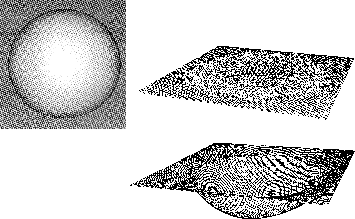
Figure 6.26:
Reconstruction of Shape From Shading: Standard Relaxation
(top right) Versus Multigrid (bottom right). The original image is
shown on left.
This case is particularly hard for a standard relaxation approach. The image
can be interpreted ``legally'' in two possible ways, as either a
concave
or
convex
hemisphere. Starting from random
initial values, after some relaxations, some image patches typically ``vote''
for one or the other interpretation and try to extend the local interpretation
to a global one. This is slow (given the local nature of the updating rule)
and encounters an endless struggle in the regions that mark the border between
different interpretations. The multigrid approach solves this ``democratic
impasse'' on the coarsest grids (much faster because information spreads over
large distances) and propagates this decision to the finer grids, that will
now concentrate their efforts on refining the initial approximation.
In Figure
6.27
, we show the reconstruction of the
Mona Lisa face painted by Leonardo da Vinci.
Figure 6.27:
Mona Lisa in Three Dimensions. The right figure shows the
multigrid reconstruction.
Next:
6.5.6 Results for Depth
Up:
A Hierarchical Scheme
Previous:
Pyramid on a
Guy Robinson
Wed Mar 1 10:19:35 EST 1995
6.5.6 Results for Depth Constraints
Next:
6.5.7 Conclusions
Up:
A Hierarchical Scheme
Previous:
6.5.5 Results for Orientation
For the surface reconstruction problem (see [
Terzopoulos:86a
]) the
energy functional is:

A physical analogy is that of fitting the depth constraints  with a
membrane pulled by springs connected to them. The effect of active
discontinuities
with a
membrane pulled by springs connected to them. The effect of active
discontinuities  is that of ``cutting the membrane'' in the proper
places.
is that of ``cutting the membrane'' in the proper
places.
Figure 6.28:
Simulation Environment for Multigrid Surface Reconstruction
from a Noisy Image. The top screen shows an intermediate, and the
bottom final results. For each screen, the upper part displays the activated
discontinuities; the lower part, the gray-encoded
z
values of the
surface.
Figure 6.29:
The Original Surface (top) and Surface Corrupted by 25%
Noise (bottom)
Figure 6.30:
The Reconstruction of a ``Randomville'' Scenery using
Multigrid Method. Each figure shows a different resolution.
Figure
6.28
to
6.30
show the simulation
environment on the SUN workstation, and the reconstruction of a
``Randomville'' image (random quadrangular blocks placed in the image
plane). The original surface, the surface corrupted by noise (25%),
are shown in Figure
6.29
while reconstruction on different
scales is shown in Figure
6.30
.
For  ``images'' and 25% noise, a faithful reconstruction of
the surface (within a few percent of the original one) is obtained after a
single multiscale sweep (with
V
cycles) on four layers. The total
computational time corresponds approximately to the time required by three
relaxations on the finest grid. Because of the optimality of multiscale
methods, time increases linearly with the number of image pixels.
``images'' and 25% noise, a faithful reconstruction of
the surface (within a few percent of the original one) is obtained after a
single multiscale sweep (with
V
cycles) on four layers. The total
computational time corresponds approximately to the time required by three
relaxations on the finest grid. Because of the optimality of multiscale
methods, time increases linearly with the number of image pixels.
Guy Robinson
Wed Mar 1 10:19:35 EST 1995
6.5.7 Conclusions
Next:
6.6 Character Recognition by
Up:
A Hierarchical Scheme
Previous:
6.5.6 Results for Depth
The parallel simulation environment was written by Roberto Battiti
[
Battiti:90a
]. Geoffrey Fox, Christof Koch, and Wojtek Furmanski
contributed with many ideas and suggestions [
Furmanski:88c
].
A JPL group [
Synnott:90a
] also used the Mark III hypercube to find
three-dimensional properties of planetary objects from the
two-dimensional images returned from NASA's planetary missions, and
from the Hubble Space Telescope. The hypercube was used in a simple
parallel mode with each node assigned calculations for a subset of the
image pixels, with no internodal communication required. The
estimation uses an iterative linear least-squares approach where the
data are the pixel brightness values in the images; and partials of
theoretical models of these brightness values are computed for use in a
square root formulation of the normal equations. The underlying
three-dimensional model of the object consists of a triaxial ellipsoid
overlaid with a spherical harmonic expansion to describe low- to
mid-spatial frequency topographic or surface composition variations.
The initial results were not followed through into production use for
JPL missions, but this is likely to become an important application of
parallel computing to image processing
from
planetary missions.
Guy Robinson
Wed Mar 1 10:19:35 EST 1995
6.6 Character Recognition by Neural Nets
Next:
6.6.1 MLP in General
Up:
6 Synchronous Applications II
Previous:
6.5.7 Conclusions
Much of the current interest in neural networks
can
be traced to the introduction a few years ago of effective learning
algorithms for these systems ([
Denker:86a
], [
Parker:82a
],
[
Rumelhart:86a
]). In [
Rumelhart:86a
] Chapter 8, it was shown
that for some problems using multi-layer perceptrons (MLP),
back-propagation
was capable of finding a
solution very reliably and quickly. Back-propagation has been applied
to a number of realistic and complex problems [
Sejnowski:87a
],
[
Denker:87a
]. The work of this section is described in
[
Felten:90a
].
Real-world problems are inherently structured, so methods incorporating this
structure will be more effective than techniques applicable to the general
case. In practice, it is very important to use whatever knowledge one has
about the form of possible solutions in order to restrict the search space.
For multilayer perceptrons, this translates into constraining the weights
or modifying the learning algorithm so as to embody the topology, geometry,
and symmetries of the problem.
Here, we are interested in determining how automatic learning can be
improved by following the above suggestion of restricting the search
space of the weights. To avoid high-level cognition requirements, we
consider the problem of classifying hand-printed upper-case Roman
characters. This is a specific pattern-recognition
problem, and has been addressed by methods other than
neural networks. Generally the recognition is separated into two
tasks: the first one is a pre-processing of the image
using translation, dilation, rotations, and so on, to bring
it to a standardized form; in the second, this preprocessed image is
compared to a set of templates and a probability is assigned to each
character or each category of the classification. If all but one of
the probabilities are close to zero, one has a high confidence level in
the identification. This second task is the more difficult one, and
the performance achieved depends on the quality of the matching
algorithm. Our focus is to study how well an MLP can learn a
satisfactory matching to templates, a task one believes the network
should be good at.
In regard to the task of preprocessing, MLPs have been shown capable
[
Rumelhart:86a
] Chapter 8 of performing translations at least in part,
but it is simpler to implement this first step using standard methods. This
combination of traditional methods and neural network matching can give us
the best of both worlds. In what follows, we suggest and test a learning
procedure which preserves the geometry of the two-dimensional image from one
length scale transformation to the next, and embodies the difference between
coarse and fine scale features.
Other References
HPFA Applications
Next:
6.6.1 MLP in General
Up:
6 Synchronous Applications II
Previous:
6.5.7 Conclusions
Guy Robinson
Wed Mar 1 10:19:35 EST 1995
6.6.1 MLP in General
Next:
6.6.2 Character Recognition using
Up:
6.6 Character Recognition by
Previous:
6.6 Character Recognition by
There are many architectures for neural networks; we shall work with
Multi-Layer Perceptrons.
These are
feed-forward networks, and the network to be used in our problem is
schematically shown in Figure
6.31
. There are two
processing layers: output and hidden. Each one has a
number of identical units (or ``neurons''), connected in a feed-forward
fashion by wires, often called weights because each one is assigned a
real number  . The input to any given unit is
  ,
where
i
labels incoming wires and
,
where
i
labels incoming wires and  is the input (or current) to
that wire. For the hidden layer,
is the input (or current) to
that wire. For the hidden layer,  is the value of a bit of the
input image; for the output layer, it is the output from a unit of
the hidden layer.
is the value of a bit of the
input image; for the output layer, it is the output from a unit of
the hidden layer.
Figure 6.31:
A Multi-Layer Perceptron
Generally, the output of a unit is a nonlinear, monotonic-increasing
function of the input. We make the usual choice and take
to be our neuron input/output function.  is the threshold and can be
different for each neuron. The weights and thresholds are usually the only
quantities which change during the learning period. We wish to have a
network perform a mapping
M
from the input space to the output space.
Introducing the actual output
is the threshold and can be
different for each neuron. The weights and thresholds are usually the only
quantities which change during the learning period. We wish to have a
network perform a mapping
M
from the input space to the output space.
Introducing the actual output  for an input
I
, one first chooses a
metric for the output space, and then seeks to minimize
for an input
I
, one first chooses a
metric for the output space, and then seeks to minimize  ,
where
d
is a measure of the distance between the two points. This quantity
is also called the error function, the energy, or (the negative of) the
harmony function. Naturally,
,
where
d
is a measure of the distance between the two points. This quantity
is also called the error function, the energy, or (the negative of) the
harmony function. Naturally,  depends on the
  's. One can then
apply standard minimization searches like simulated annealing
[
Kirkpatrick:83a
] to attempt to change the
's. One can then
apply standard minimization searches like simulated annealing
[
Kirkpatrick:83a
] to attempt to change the  's so
as to reduce the error. The most commonly used method is gradient
descent, which for MLP is called
back-propagation
because the calculation of the
gradients is performed in a feed-backwards fashion. Improved descent
methods may be found in [
Dahl:87a
], [
Parker:87a
] and in
Section
9.9
of this book.
's so
as to reduce the error. The most commonly used method is gradient
descent, which for MLP is called
back-propagation
because the calculation of the
gradients is performed in a feed-backwards fashion. Improved descent
methods may be found in [
Dahl:87a
], [
Parker:87a
] and in
Section
9.9
of this book.
The minimization often runs into difficulties because one is searching in a
very high-dimensional space, and the minima may be narrow. In addition,
the straightforward implementation of back-propagation will often fail
because of the many minima in the energy landscape. This process of
minimization is referred to as learning or memorization as the network tries
to match the mapping
M
. In many problems, though, the input space is so
huge that it is neither conceivable nor desirable to present all possible
inputs to the network for it to memorize. Given part of the mapping
M
, the
network is expected to guess the rest: This is called generalization. As
shown clearly in [
Denker:87a
] for the case of a discrete input space,
generalization is often an ill-posed problem: Many generalizations of
M
are possible. To achieve the kind of generalization humans want, it is
necessary to tell the network about the mapping one has in mind. This is
most simply done by constraining the weights to have certain symmetries as in
[
Denker:87a
]. Our approach will be similar, except that the ``outside''
information will play an even more central role during the learning process.
Next:
6.6.2 Character Recognition using
Up:
6.6 Character Recognition by
Previous:
6.6 Character Recognition by
Guy Robinson
Wed Mar 1 10:19:35 EST 1995
6.6.2 Character Recognition using MLP
Next:
6.6.3 The Multiscale Technique
Up:
6.6 Character Recognition by
Previous:
6.6.1 MLP in General
To do character recognition
using an MLP,
we assume the input layer of the network to be a set of image pixels,
which can take on analogue (or grey scale) values between 0 and 1. The
two-dimensional set of pixels is mapped onto the set of input neurons
in a fairly arbitrary way: For an  image, the top row of
N
pixels is associated with the first
N
neurons, the next row of
N
pixels is associated with the next
N
neurons, and so forth. At
the start of the training process, the network has no knowledge of the
underlying two-dimensional structure of the problem (that is, if a
pixel is on, nearby pixels in the two-dimensional space are also likely
to be on). The network discovers the two-dimensional nature of the
problem during the learning process.
image, the top row of
N
pixels is associated with the first
N
neurons, the next row of
N
pixels is associated with the next
N
neurons, and so forth. At
the start of the training process, the network has no knowledge of the
underlying two-dimensional structure of the problem (that is, if a
pixel is on, nearby pixels in the two-dimensional space are also likely
to be on). The network discovers the two-dimensional nature of the
problem during the learning process.
We taught our networks the alphabet of 26 upper-case Roman characters. To
encourage generalization, we show the net many different hand-drawn versions
of each character. The 320-image training set is shown in
Figure
6.32
. These images were hand-drawn using a mouse attached
to a SUN workstation. The output is encoded in a very sparse way. There are
only 26 outputs we want the net to give, so we use 26 output neurons and map
the output pattern: first neuron on, rest off, to the character ``A;''
second neuron on, rest off, to ``B;'' and so on. Such an encoding
scheme works well here, but is clearly unworkable for mappings with large
output sets such as Chinese characters or Kanji. In such cases, one would
prefer a more compact output encoding, with possibly an additional layer of
hidden units to produce the more complex outputs.
Figure 6.32:
The Training Set of 320 Handwritten Characters, Digitized on a
 Grid
Grid
As mentioned earlier, we do not feed images directly into the network.
Instead, simple, automatic preprocessing is done which dilates the image to
a standard size and then translates it to the center of the pixel space.
This greatly enhances the performance of the system-it means that one can
draw a character in the upper left-hand corner of the pixel space and the
system easily recognizes it. If we did not have the preprocessing, the
network would be forced to solve the much larger problem of character
recognition of all possible sizes and locations in the pixel space. Two
other worthwhile preprocessors are rotations (rotate to a standard
orientation) and intensity normalization (set linewidths to some standard
value). We do not have these in our current implementation.
The MLP is used only for the part of the algorithm where one matches to
templates. Given any fixed set of exemplars, a neural network will usually
learn this set perfectly, but the performance under generalization can be
very poor. In fact, the more weights there are, the faster the learning (in
the sense of number of iterations, not of CPU time), and the
worse the ability to generalize. This was in part realized in
[
Gullichsen:87a
], where the input grid was  . If one has a
very fine mesh at the input level, so that a great amount of detail can be
seen in the image, one runs the risk of having terrible generalization
properties because the network will tend to focus upon tiny features of the
image, ones which humans would consider irrelevant.
. If one has a
very fine mesh at the input level, so that a great amount of detail can be
seen in the image, one runs the risk of having terrible generalization
properties because the network will tend to focus upon tiny features of the
image, ones which humans would consider irrelevant.
We will show one approach to overcoming this problem. We desire the
potential power of the large, high-resolution net, but with the stable
generalization properties of small, coarse nets. Though not so important for
upper-case Roman characters, where a rather coarse grid does well enough (as
we will see), a fine mesh is necessary for other problems such as recognition
of Kanji characters or handwriting. A possible ``fix,'' similar to what was
done for the problem of clump counting [
Denker:87a
], is to
hard wire the first layer of weights to be local in space, with a
neighborhood growing with the mesh fineness. This reduces the number of
weights, thus postponing the deterioration of the generalization. However,
for an MLP with a single hidden layer, this approach will prevent the
detection of many nonlocal correlations in the images, and in effect this
fix is like removing the first layer of weights.
Next:
6.6.3 The Multiscale Technique
Up:
6.6 Character Recognition by
Previous:
6.6.1 MLP in General
Guy Robinson
Wed Mar 1 10:19:35 EST 1995
6.6.3 The Multiscale Technique
Next:
6.6.4 Results
Up:
6.6 Character Recognition by
Previous:
6.6.2 Character Recognition using
We would like to train large, high-resolution nets. If one tries to do this
directly, by simply starting with a very large network and training by the
usual back-propagation methods, not only is the training slow (because of the
large size of the network), but the generalization properties of such nets are
poor. As described above, a large net with many weights from the input layer
to the hidden layer tends to ``grandmother'' the problem, leading to poor
generalization.
The hidden units of an MLP form a set of feature extractors. Considering a
complex pattern such as a Chinese character, it seems clear that some of the
relevant features which distinguish it are large, long-range objects
requiring little detail while other features are fine scale and require high
resolution. Some sort of multiscale decomposition of the problem therefore
suggests itself. The method we will present below builds in long-range
feature extractors by training on small networks and then uses these as an
intelligent starting point on larger, higher resolution networks. The method
is somewhat analogous to the multigrid technique for solving partial
differential equations.
Let us now present our multiscale training algorithm. We begin with the
training set, such as the one shown in Figure
6.32
, defined at the
high resolution (in this case,  ). Each exemplar is coarsened by
a factor of two in each direction using a simple grey scale averaging
procedure.
). Each exemplar is coarsened by
a factor of two in each direction using a simple grey scale averaging
procedure.  blocks of pixels in which all four pixels were ``on''
map to an ``on'' pixel, those in which three of the four were ``on'' map to
a ``3/4 on'' pixel, and so on. The result is that each
blocks of pixels in which all four pixels were ``on''
map to an ``on'' pixel, those in which three of the four were ``on'' map to
a ``3/4 on'' pixel, and so on. The result is that each  exemplar is mapped to a
  exemplar in such a way as to preserve
the large scale features of the pattern. The procedure is then repeated
until a suitably coarse representation of the exemplars is reached. In our
case, we stopped after coarsening to
exemplar in such a way as to preserve
the large scale features of the pattern. The procedure is then repeated
until a suitably coarse representation of the exemplars is reached. In our
case, we stopped after coarsening to  .
.
At this point, an MLP is trained to solve the coarse mapping problem by
one's favorite method (back-propagation, simulated annealing, and so on).
In our case, we set up an MLP of 64 inputs (corresponding to  ), 32 hidden units, and 26 output units. This was then trained on
the set of 320 coarsened exemplars using the simple back propagation
method with a momentum term [
Rumelhart:86a
], Chapter 8.
Satisfactory convergence
was achieved after
approximately 50 cycles through the training set.
), 32 hidden units, and 26 output units. This was then trained on
the set of 320 coarsened exemplars using the simple back propagation
method with a momentum term [
Rumelhart:86a
], Chapter 8.
Satisfactory convergence
was achieved after
approximately 50 cycles through the training set.
We now wish to boost back to a high-resolution MLP, using the results of the
coarse net. We use a simple interpolating procedure which works well. We
leave the number of hidden units unchanged. Each weight from the input layer
to the hidden layer is split or ``un-averaged'' into four weights (each now
attached to its own pixel), with each 1/4 the size of the original. The
thresholds are left untouched during this boosting phase. This procedure
gives a higher resolution MLP with an intelligent starting point for
additional training at the finer scale. In fact, before any training at
all is done with the  MLP (boosted from
  ), it recalls
the
), it recalls
the  exemplars quite well. This is a measure of how much
information was lost when coarsening from
exemplars quite well. This is a measure of how much
information was lost when coarsening from  to
to  . The
boost and train process is repeated to get to the desired
. The
boost and train process is repeated to get to the desired  MLP.
The entire multiscale training process is illustrated in
Figure
6.33
.
MLP.
The entire multiscale training process is illustrated in
Figure
6.33
.
Figure 6.33:
An Example Flowchart for the Multiscale Training Procedure.
This was the procedure used in this text, but the averaging and boosting
can be continued through an indefinite number of stages.
Next:
6.6.4 Results
Up:
6.6 Character Recognition by
Previous:
6.6.2 Character Recognition using
Guy Robinson
Wed Mar 1 10:19:35 EST 1995
6.6.4 Results
Next:
6.6.5 Comments and Variants
Up:
6.6 Character Recognition by
Previous:
6.6.3 The Multiscale Technique
Here we give some details of our results and compare with the standard
approach. As mentioned in the previous section, a  MLP (1024
inputs, 32 hidden units, 26 output units) was trained on the set of
Figure
6.32
using the multiscale method. Outputs are never
exactly 0 or 1, so we defined a ``successful'' recognition to occur when the
output value of the desired letter was greater than 0.9, and all other
outputs were less than 0.1. The training on the
MLP (1024
inputs, 32 hidden units, 26 output units) was trained on the set of
Figure
6.32
using the multiscale method. Outputs are never
exactly 0 or 1, so we defined a ``successful'' recognition to occur when the
output value of the desired letter was greater than 0.9, and all other
outputs were less than 0.1. The training on the  grid used
back-propagation with a momentum term and went through the exemplars
sequentially. The weights are changed to reduce the error function for
the current character. The result is that the system does not reach an
absolute minimum. Rather, at long times the weight values oscillate with a
period equal to the time of one sweep through all the exemplars. This is not
a serious problem as the oscillations are very small in practice.
Figure
6.34
shows the training curve for this problem. The first
part of the curve is the training of the
grid used
back-propagation with a momentum term and went through the exemplars
sequentially. The weights are changed to reduce the error function for
the current character. The result is that the system does not reach an
absolute minimum. Rather, at long times the weight values oscillate with a
period equal to the time of one sweep through all the exemplars. This is not
a serious problem as the oscillations are very small in practice.
Figure
6.34
shows the training curve for this problem. The first
part of the curve is the training of the  network; even though the
grid is a bit coarse, almost all of the characters can be memorized.
Proceeding to the next grid by scaling the mesh size by a factor of two and
using the
network; even though the
grid is a bit coarse, almost all of the characters can be memorized.
Proceeding to the next grid by scaling the mesh size by a factor of two and
using the  exemplars, we obtained the second part of the
learning curve in Figure
6.34
. The
exemplars, we obtained the second part of the
learning curve in Figure
6.34
. The  net got 315/320
correct. After 12 additional sweeps on the
net got 315/320
correct. After 12 additional sweeps on the  net, a perfect
score of 320/320 is achieved. The third part of Figure
6.34
shows
the result of the final boost to
net, a perfect
score of 320/320 is achieved. The third part of Figure
6.34
shows
the result of the final boost to  . In just two cycles on the
 net, a perfect score of 320/320 was achieved and the training
was stopped. It is useful to compare these results with a direct use of
back-propagation on the
net, a perfect score of 320/320 was achieved and the training
was stopped. It is useful to compare these results with a direct use of
back-propagation on the  mesh without using the multiscale
procedure. Figure
6.35
shows the corresponding learning curve,
with the result from Figure
6.34
drawn in for comparison.
Learning via the multiscale method takes much less computer time. In
addition, the internal structure of the resultant network is much different
and we will now turn to this question.
mesh without using the multiscale
procedure. Figure
6.35
shows the corresponding learning curve,
with the result from Figure
6.34
drawn in for comparison.
Learning via the multiscale method takes much less computer time. In
addition, the internal structure of the resultant network is much different
and we will now turn to this question.
How do these two networks compare for the real task of recognizing exemplars
not belonging to the training set? We used as a generalization test set 156
more handwritten characters. Though there are no ambiguities for humans in
this test set, the networks did make mistakes. The network from the direct
method made errors 14% of the time, and the multiscale network made errors
9% of the time. We feel the improved performance of the multiscale net is
due to the difference in quality of the feature extractors in the two cases.
In a two-layer MLP, we can think of each hidden-layer neuron as a feature
extractor which looks for a certain characteristic shape in the input; the
function of the output layer is then to perform the higher level operation of
classifying the input based on which features it contains. By looking at the
weights connecting a hidden-layer neuron to the inputs, we can determine
what feature that neuron is looking for.
Figure 6.34:
The Learning Curve for our Multiscale Training Procedure
Applied to 320 Handwritten Characters. The first part of the curve is
the training on the  net, the second on the
  net, and the last on the full,
  net. The curve is plotted
as a function of CPU time and not sweeps through the presentation set,
in order to exhibit the speed of training on the smaller networks.
net. The curve is plotted
as a function of CPU time and not sweeps through the presentation set,
in order to exhibit the speed of training on the smaller networks.
Figure:
A Comparison of Multiscale Training with the Usual, Direct
Back-propagation Procedure. The curve labelled ``Multiscale'' is the same as
Figure
6.34
, only rescaled by a factor of two. The curve
labelled ``Brute Force'' is from directly training a  network,
from a random start, on the learning set. The direct approach does not quite
learn all of the exemplars, and takes much more CPU time.
network,
from a random start, on the learning set. The direct approach does not quite
learn all of the exemplars, and takes much more CPU time.
For example, Figure
6.36
shows the input weights of two neurons in
the  net. The neuron of (a) seems to be looking for a stroke
extending downward and to the right from the center of the input field. This
is a feature common to letters like A, K, R, and X. The feature extractor of
(b) seems to be a ``NOT S'' recognizer and, among other things, discriminates
between ``S'' and ``Z''.
net. The neuron of (a) seems to be looking for a stroke
extending downward and to the right from the center of the input field. This
is a feature common to letters like A, K, R, and X. The feature extractor of
(b) seems to be a ``NOT S'' recognizer and, among other things, discriminates
between ``S'' and ``Z''.
Figure 6.36:
Two Feature Extractors for the Trained  net. This figure
shows the connection weights between one hidden-layer, and all the
input-layer neurons. Black boxes depict positive weights, while white
depict negative weights; the size of the box shows the magnitude. The
position of each weight in the
net. This figure
shows the connection weights between one hidden-layer, and all the
input-layer neurons. Black boxes depict positive weights, while white
depict negative weights; the size of the box shows the magnitude. The
position of each weight in the  grid corresponds to the position
of the input pixel. We can view these pictures as maps of the features which
each hidden-layer neuron is looking for. In (a), the neuron is looking for a
stroke extending down and to the right from the center of the input field;
this neuron fires upon input of the letter ``A,'' for example. In (b), the
neuron is looking for something in the lower center of the picture, but it
also has a strong ``NOT S'' component. Among other things, this neuron
discriminates between an ``S'' and a ``Z''. The outputs of several such
feature extractors are combined by the output layer to classify the original
input.
grid corresponds to the position
of the input pixel. We can view these pictures as maps of the features which
each hidden-layer neuron is looking for. In (a), the neuron is looking for a
stroke extending down and to the right from the center of the input field;
this neuron fires upon input of the letter ``A,'' for example. In (b), the
neuron is looking for something in the lower center of the picture, but it
also has a strong ``NOT S'' component. Among other things, this neuron
discriminates between an ``S'' and a ``Z''. The outputs of several such
feature extractors are combined by the output layer to classify the original
input.
Figure:
The Same Feature Extractor as in Figure
6.36
(b),
after the Boost to  . There is an obvious correspondence between
each connection in Figure
6.36
(b) and
. There is an obvious correspondence between
each connection in Figure
6.36
(b) and  clumps
of connections here. This is due to the multiscale procedure, and leads to
spatially smooth feature extractors.
clumps
of connections here. This is due to the multiscale procedure, and leads to
spatially smooth feature extractors.
Even at the coarsest scale, the feature extractors usually look for blobs
rather than correlating a scattered pattern of pixels. This is encouraging
since it matches the behavior we would expect from a ``good'' character
recognizer. The multiscale process accentuates this locality, since a single
pixel grows to a local clump of four pixels at each rescaling. This effect
can be seen in Figure
6.37
, which shows the feature extractor of
Figure
6.36
(b) after scaling to  and further
training. Four-pixel clumps are quite obvious in the
and further
training. Four-pixel clumps are quite obvious in the  network.
The feature extractors obtained by direct training on large nets are much
more scattered (less smooth) in nature.
network.
The feature extractors obtained by direct training on large nets are much
more scattered (less smooth) in nature.
Next:
6.6.5 Comments and Variants
Up:
6.6 Character Recognition by
Previous:
6.6.3 The Multiscale Technique
Guy Robinson
Wed Mar 1 10:19:35 EST 1995
6.6.5 Comments and Variants on the Method
Next:
An Adaptive Multiscale
Up:
6.6 Character Recognition by
Previous:
6.6.4 Results
Before closing, we would like to make some additional comments on the
multiscale method and suggest some possible extensions.
In a pattern-recognition problem such as character recognition, the
two-dimensional spatial structure
of the
problem is important. The multiscale method preserves this structure
so that ``reasonable'' feature extractors are produced. An obvious
extension to the present work is to increase the number of hidden units
as one boosts the MLP to higher resolution. This corresponds to adding
completely new feature extractors. We did not do this in the present
case since 32 hidden units were sufficient-the problem of recognizing
upper-case Roman characters is too easy. For a more challenging
problem such as Chinese characters, adding hidden units will probably
be necessary. We should mention that incrementally adding hidden units
is easy to do and works well-we have used it to achieve perfect
convergence
of a back-propagation network for the
problem of tic-tac-toe.
When boosting, the weights are scaled down by a factor of four and so it is
important to also scale down the learning rate (in the back-propagation
algorithm) by a factor of four.
We defined our ``blocking,''
or coarsening, procedure to
be a simple, grey scale averaging of  blocks. There are
many other possibilities, well known in the field of real-space
renormalization in physics. Other interesting blocking
procedures include: using a scale factor,
blocks. There are
many other possibilities, well known in the field of real-space
renormalization in physics. Other interesting blocking
procedures include: using a scale factor,  , different from
two; using majority rule averaging; simple decimation; and so on.
, different from
two; using majority rule averaging; simple decimation; and so on.
Multiscale methods work well in cases where spatial locality or smoothness
is relevant (otherwise, the interpolation approximation is bad). Another way
of thinking about this is that we are decomposing the problem onto a set of
spatially local basis functions such as gaussians. In other problems, a
different set of basis functions may be more appropriate and hence give better
performance.
The multiscale method uses results from a small net to help in the training
of a large network. The different-sized networks are related by the
rescaling or dilation operator. A variant of this general approach would be
to use the translation operator to produce a pattern matcher for the game of
Go. The idea is that at least
some
of the complexity of Go is
concerned with local strategies. Instead of training an MLP to learn this on
the full  board of Go, do the training on a ``mini-Go'' board of
 or
or  . The appropriate way to relate these networks to
the full-sized one is not through dilations, but via the translations: The
same local strategies are valid everywhere on the board.
. The appropriate way to relate these networks to
the full-sized one is not through dilations, but via the translations: The
same local strategies are valid everywhere on the board.
Steve Otto had the original idea for the MultiScale training technique. Otto
and Ed Felten and Olivier Martin developed the method. Jim Hutchinson
contributed by supplying the original back-propagation program.
Next:
An Adaptive Multiscale
Up:
6.6 Character Recognition by
Previous:
6.6.4 Results
Guy Robinson
Wed Mar 1 10:19:35 EST 1995
An Adaptive Multiscale Scheme for
Real-Time Motion Field Estimation
Next:
6.7.1 Errors in Computing
Up:
6 Synchronous Applications II
Previous:
6.6.5 Comments and Variants
When moving objects in a scene are projected onto an image
plane (for example, onto our retina), the real velocity field is
transformed into a two-dimensional field, known as the
motion
field.
By taking more images at different times and calculating the motion field, we
can extract useful parameters like the time to collision, useful for obstacle
avoidance. If we know the motion of a camera (or our ego motion), we can
reconstruct the entire three-dimensional structure of the environment (if the
camera translates, near objects will have a larger motion field with respect
to distant ones). The depth measurements can be used as starting constraints
for a surface reconstruction algorithm like the one described in
Section
9.9
.
In particular situations, the apparent motion of the brightness pattern,
known as the optical flow,
provides a sufficiently
accurate estimate of the
motion field. Although the adaptive scheme that we propose is applicable to
different methods, the discussion will be based on the scheme proposed by
Horn and Schunck [
Horn:81a
]. They use the assumptions that the image
brightness of a given point remains constant over time, and that the optical
flow varies smoothly almost everywhere. Satisfaction of these two
constraints is formulated as the problem of minimizing a quadratic energy
functional (see also [
Poggio:85a
]). The appropriate Euler-Lagrange
equations are then discretized on a single or multiple grid and solved using,
for example, the Gauss-Seidel relaxation method [
Horn:81a
],
[
Terzopoulos:86a
]). The resulting system of equations (two for
every pixel in the image) is:


where  and
and  are the optical
flow variables to be determined,
are the optical
flow variables to be determined,  ,
,  ,
,  are the partial
derivatives of the image brightness with respect to space and time,
are the partial
derivatives of the image brightness with respect to space and time,  and
and  are local averages,
  is the spatial discretization
step, and
is the spatial discretization
step, and  controls the smoothness of the estimated optical flow.
Other References
HPFA Applications
Next:
6.7.1 Errors in Computing
Up:
6 Synchronous Applications II
Previous:
6.6.5 Comments and Variants
Guy Robinson
Wed Mar 1 10:19:35 EST 1995
6.7.1 Errors in Computing the Motion Field
Next:
6.7.2 Adaptive Multiscale Scheme
Up:
An Adaptive Multiscale
Previous:
An Adaptive Multiscale
Now, we need to estimate the partial derivatives in the above equations with
discretized formulas
starting from brightness values that are
quantized
(say integers from 0 to
n
) and noisy. Given these
derivative estimation problems, the optimal step for the discretization grid
depends on local properties of the image. Use of a single discretization
step produces large errors on some images. Use of a
homogeneous
multiscale approach, where a set of grids at different resolutions is
used, may in some cases produce a good estimation on an intermediate
grid and a bad one on the final and finest grid. Enkelmann and Glazer
[
Enkelmann:88a
], [
Glazer:84a
] encountered similar problems.
These difficulties can be illustrated with the following one-dimensional
example. Let's suppose that the intensity pattern observed is a
superposition of two sinusoids of different wavelengths:

where
R
is the ratio of short to long wavelength components. Using the
brightness constancy
assumption ( or
or  , see [
Horn:81a
]) the measured velocity
, see [
Horn:81a
]) the measured velocity  is
given by:
is
given by:

where  and
and  are the three-point approximations
of the spatial and temporal brightness derivatives.
are the three-point approximations
of the spatial and temporal brightness derivatives.
Now, if we calculate the estimated velocity on two different grids, with
spatial step  equal to one and two, as a function of the parameter,
R
, we obtain the result illustrated in Figure
6.38
.
equal to one and two, as a function of the parameter,
R
, we obtain the result illustrated in Figure
6.38
.
Figure 6.38:
Measured velocity for superposition of sinusoidal patterns as a
function of the ratio of short to long wavelength components. Dashed line:
 , continuous line:
  .
.
While on the coarser grid, the correct velocity is obtained (in this case);
on the finer one, the measured velocity depends on the value of
R
. In
particular, if
R
is greater than  , we obtain a velocity in the
opposite direction!
, we obtain a velocity in the
opposite direction!
We propose a method for ``tuning'' the discretization grid to a measure of
the reliability of the optical flow
derived at a given
scale. This measure
is based on a
local estimate of the errors
due to noise and
discretization, and is described in
[Battiti:89g;91b].
Next:
6.7.2 Adaptive Multiscale Scheme
Up:
An Adaptive Multiscale
Previous:
An Adaptive Multiscale
Guy Robinson
Wed Mar 1 10:19:35 EST 1995
6.7.2 Adaptive Multiscale Scheme on a Multicomputer
Next:
6.7.3 Conclusions
Up:
An Adaptive Multiscale
Previous:
6.7.1 Errors in Computing
First, a Gaussian pyramid
[
Burt:84a
] is
computed from the given images.
This consists of a hierarchy of images obtained filtering the original ones
with Gaussian filters of progressively larger size.
Then, the optical flow field is computed at the coarsest scale using
relaxation, and the estimated error is calculated for every pixel. If this
quantity is less than a given threshold  , the current value of the
flow is interpolated to the finer resolutions without further processing.
This is done by setting an
inhibition flag
contained in the grid
points of the pyramidal structure, so that these points do not participate in
the relaxation process. On the contrary, if the error is larger than
, the current value of the
flow is interpolated to the finer resolutions without further processing.
This is done by setting an
inhibition flag
contained in the grid
points of the pyramidal structure, so that these points do not participate in
the relaxation process. On the contrary, if the error is larger than
 , the approximation is relaxed on a finer scale and the entire
process is repeated until the finest scale is reached.
, the approximation is relaxed on a finer scale and the entire
process is repeated until the finest scale is reached.
Figure 6.39:
Adaptive Grid (shown on left) in the Multiresolution
Pyramid; (middle) Gray Code Mapping Strategy; (right) Domain
Decomposition Mapping Strategy. In the middle and right pictures, the
activity pattern for three resolutions is shown at the top, for a
simple one-dimensional case.
In this way, we obtain a
local inhomogeneous
approach where areas of
the images, characterized by different spatial frequencies or by different
motion amplitudes, are processed at the appropriate resolutions, avoiding
corruption of good estimates by inconsistent information from a different
scale (the effect shown in the previous example). The optimal grid
structure for a given image is translated into a pattern of active and
inhibited
grid points in the pyramid,
as
illustrated in Figure
6.39
.
Figure 6.40:
Efficiency and Solution Times
The motivation for
freezing
the motion field as soon as the error is
below threshold, is that the estimation of the error may
itself
become incorrect at finer scales and, therefore, useless in the decision
process. It is important to point out that single-scale or homogeneous
approaches cannot adequately solve the above problem. Intuitively, what
happens in the adaptive multiscale approach is that the velocity is
frozen
as soon as the spatial and temporal differences at a given
scale are big enough to avoid quantization errors, but small enough to avoid
errors in the use of discretized formulas. The only assumption made in this
scheme is that the largest motion in the scene can be reliably computed at
one of the used resolutions. If the images contain motion
discontinuities,
line processes
(indicating the presence of these discontinuities) are necessary to
prevent smoothing where it is not desired (see [
Battiti:90a
] and
the contained references).
Figure 6.41:
Plaid Image (top); The Error in Calculation of Optical Flow
for both Homogeneous (Upper-line) and Adaptive (Lower-line) Algorithms.
The error is plotted as a function of computation time.
Figure:
Reconstructed Optical Flow for Translating ``Plaid'' Pattern
of Figure
6.41
. Homogeneous Multiscale Strategy
(top), Adaptive Multiscale Strategy (middle), and Active (black) and
Inhibited (white) Points
Figure 6.43:
Test Images and Motion Fields for a Natural (pine-cone) Image
at Three Resolutions (top). Estimated versus Actual Velocity Plotted
for Three Choices of Resolution (bottom). The dotted line indicates a
``perfect'' prediction.
Large grain-size multicomputers, with a mapping based on domain
decomposition and limited coarsening, have been used to implement the
adaptive algorithm, as described in Section
6.5
. The efficiency
and solution times for an implementation with
transputers
(details in [
Battiti:91a
]) are
shown in Figure
6.40
.
Real-time computation with high efficiency is within the reach of available
digital technology!
On a board with four transputers, and using the Express communication
routines from ParaSoft, the solution time for  images is on
the order of one second.
images is on
the order of one second.
The software implementation is based on the multiscale vision environment
developed by Roberto Battiti and described in Section
9.9
.
Christof Koch and Edoardo Amaldi collaborated on the project.
Next:
6.7.3 Conclusions
Up:
An Adaptive Multiscale
Previous:
6.7.1 Errors in Computing
Guy Robinson
Wed Mar 1 10:19:35 EST 1995
6.7.3 Conclusions
Next:
6.8 Collective Stereopsis
Up:
An Adaptive Multiscale
Previous:
6.7.2 Adaptive Multiscale Scheme
Results of the algorithm show that the adaptive method is capable of
effectively reducing the solution error. In the last Figures
6.41
to
6.43
, we show two test images (showing a ``plaid''
pattern and a natural scene), with the obtained optical flow.
For the ``plaid'' image, we show the r.m.s. error obtained with the adaptive
(lower-line) and homogeneous (upper-line) scheme and the resulting fields.
For the natural image, we show in Figure
6.42
, the average
computed velocity (in a region centered on the pine cone) as a function
of the correct velocity for different number of layers. Increasing the
number of resolution grids increases the range of velocities that are
detected correctly by the algorithm. The pine cone is moving upward
at the rate of 1.6 pixels per frame. The
multiscale
algorithm is always better than
single-level algorithm, especially at larger velocity  .
.
Guy Robinson
Wed Mar 1 10:19:35 EST 1995
6.8 Collective Stereopsis
Next:
7 Independent Parallelism
Up:
6 Synchronous Applications II
Previous:
6.7.3 Conclusions
The collective stereopsis
algorithm described in
[
Marr:76a
] was historically one of the first ``cooperative''
algorithms based on relaxation proposed for early vision.
The goal in stereopsis is to measure the difference in retinal position
(
disparity
) of features of a scene observed with two eyes (or
video cameras). This is achieved by placing a fiber of ``neurons''
(one for each disparity value) at each pixel position. Each neuron
inhibits neurons of different disparities at the same location (because
the disparity is unique) and excites neurons of the same disparity at
near location (because disparity tends to vary smoothly). After,
convergence
the activation pattern corresponds to
the disparity field defined above.
Figure 6.44:
Collective Stereopsis: (top left) Definition for geometry of
stereoscopic vision. (bottom left) Neural Network Activity (top three
layers disparity
d=0, 1, 2
) corresponding to real world
structure illustrated. (right) Results of iterations for
d=0
and
d=2
layers of neurons.
d
measures disparity value for pixels.
The parallel implementation is based on a straightforward domain
decomposition and the results are illustrated in
Figure
6.44
. They show the initial state of disparity
computation and the evolution in time of the different layers of
disparity neurons. Details are described in [
Battiti:88a
].
Other References
HPFA Applications
Guy Robinson
Wed Mar 1 10:19:35 EST 1995
7 Independent Parallelism
Next:
7.1 Embarrassingly Parallel Problem
Up:
Parallel Computing Works
Previous:
6.8 Collective Stereopsis
Guy Robinson
Wed Mar 1 10:19:35 EST 1995
7.1 Embarrassingly Parallel Problem Structure
Next:
7.2 Dynamically Triangulated Random
Up:
7 Independent Parallelism
Previous:
7 Independent Parallelism
In Chapters
4
and
6
, we studied the
synchronous
problem class where the uniformity of the computation,
that is, of the
temporal
structure, made the parallel
implementation relatively straightforward. This chapter contains
examples of the other major problem class, where the simple
spatial
structure leads to clear parallelization. We define the
embarrassingly parallel
class of
problems for which the computational graph
is disconnected. This spatial structure
allows a simple parallelization as no (temporal) synchronization is
involved. In Chapters
4
and
6
, on the other
hand, there was often substantial synchronization and associated
communication; however, the uniformity of the synchronization allowed
a clear parallelization strategy. One important feature of
embarrassingly parallel problems is the modest node-to-node
communication requirements-the definition of no spatial connection
implies in fact no internode communication, but a practical problem
would involve some amount of communication, if only to set up the
problem and accumulate results. The low communication requirements of
embarrassingly parallel problems make them particularly suitable for a
distributed computing implementation on a network of workstations;
even the low bandwidth
of an Ethernet is often
sufficient. Indeed, we used such a network of Sun workstations to
support some of the simulations described in Section
7.2
.
The caricature of this problem class, shown in Figure
7.1
,
uses a database problem as an example. This is illustrated in practice
by the DOWQUEST program where a CM-2 supports searching of financial
data contained in articles that are partitioned equally over the nodes
of this SIMD machine
[Waltz:87a;88a,90a].
Figure 7.1:
Embarrassingly Parallel Problem Class
This problem class can have either a synchronous or asynchronous
temporal structure.
We have illustrated the
former above and analysis of a large (high energy) physics data set
exhibits asynchronous temporal structure. Such experiments can record
 -
- separate events, which can be analyzed independently.
However, each event is usually quite different and would require both
distinct instruction streams and very different execution times. This
was realized early in the high energy physics
community and so-called farms-initially of special-purpose
machines and now of commercial workstations-have been used
extensively for production data analysis
[
Gaines:87a
], [
Hey:88a
], [
Kunz:81a
].
separate events, which can be analyzed independently.
However, each event is usually quite different and would require both
distinct instruction streams and very different execution times. This
was realized early in the high energy physics
community and so-called farms-initially of special-purpose
machines and now of commercial workstations-have been used
extensively for production data analysis
[
Gaines:87a
], [
Hey:88a
], [
Kunz:81a
].
The applications in Sections
7.2
and
7.6
obtain their
embarrassingly parallel structure from running several full
simulations-each with independent data. Each simulation could in
fact also be decomposed spatially and in fact this spatial
parallelization has since been pursued and is described for the neural
network simulator in Section
7.6
. Some of Chiu's random block
lattice calculations also used an embarrassingly parallel approach with
1024 separate  lattices being calculated on the 1024
nCUBE-1
at Sandia [
Chiu:90a
],
[Fox:89i;89n]. This would not, of course, be possible
for the QCD of Section
4.3
, where each node would not be
available to hold an interesting size lattice. The spatial parallelism
in the examples of Sections
7.2
and
7.6
is nontrivial
to implement as the irregularities makes these problems loosely
synchronous. This relatively difficult domain parallelism made it
attractive to first explore the independent structure gotten by
exploiting the parallelism coming from simulations with different
parameters.
lattices being calculated on the 1024
nCUBE-1
at Sandia [
Chiu:90a
],
[Fox:89i;89n]. This would not, of course, be possible
for the QCD of Section
4.3
, where each node would not be
available to hold an interesting size lattice. The spatial parallelism
in the examples of Sections
7.2
and
7.6
is nontrivial
to implement as the irregularities makes these problems loosely
synchronous. This relatively difficult domain parallelism made it
attractive to first explore the independent structure gotten by
exploiting the parallelism coming from simulations with different
parameters.
It is interesting that Sections
6.3
and
7.3
both
address simulations of spin systems relevant to high  -depending
on the algorithm used, one can get very different problem
architectures
(either synchronous or
embarrassingly parallel in this case) for a given application.
-depending
on the algorithm used, one can get very different problem
architectures
(either synchronous or
embarrassingly parallel in this case) for a given application.
The embarrassingly parallel gravitational lens application of
Section
7.4
was frustrating for the developers as it needed
software support not available at the time on the Mark III. Suitable
software (MOOSE in Section
15.2
) had been developed on the
Mark II to support graphics ray tracing
as briefly
discussed in Section
14.1
. Thus, the calculation is
embarrassingly parallel, but a distributed database is essentially
needed to support the calculation of each ray. This was not available
in CrOS III at the time of the calculations described in
Section
7.4
.
Next:
7.2 Dynamically Triangulated Random
Up:
7 Independent Parallelism
Previous:
7 Independent Parallelism
Guy Robinson
Wed Mar 1 10:19:35 EST 1995
7.2 Dynamically Triangulated Random Surfaces
Next:
7.2.1 Introduction
Up:
7 Independent Parallelism
Previous:
7.1 Embarrassingly Parallel Problem
Other References
HPFA Paradigms
Guy Robinson
Wed Mar 1 10:19:35 EST 1995
7.2.1 Introduction
Next:
7.2.2 Discretized Strings
Up:
7.2 Dynamically Triangulated Random
Previous:
7.2 Dynamically Triangulated Random
In this section, we describe some large scale parallel simulations of
dynamically triangulated
random
surfaces
[
Baillie:90c
], [
Baillie:90d
],
[
Baillie:90e
], [
Baillie:90j
], [
Baillie:91c
],
[
Bowick:93a
]. Dynamically triangulated random surfaces have been
suggested as a possible discretization for string theory
in high energy physics and fluid surfaces or
membranes
in biology
[
Lipowski:91a
]. As physicists, we shall focus on the former.
String theories describe the interaction of one-dimensional string-like
objects in a fashion analogous to the way particle theories describe the
interaction of zero-dimensional point-like particles. String theory has its
genesis in the dual models that were put forward in the 1960s to describe
the behavior of the hadronic spectrum then being observed. The dual model
amplitudes could be derived from the quantum theory of a stringlike object
[
Nambu:70a
], [
Nielsen:70a
], [
Susskind:70a
]. It was later
discovered that these so-called bosonic strings could apparently only live in
26 dimensions [
Lovelace:68a
] if they were to be consistent
quantum-mechanically. They also had tachyonic (negative mass-squared) ground
states, which is normally the sign of an instability. Later, fermionic
degrees of freedom were added to the theory, yielding the supersymmetric
Neveu-Schwarz-Ramond [
Neveu:71a
] (NSR) string. This has a critical
dimension of 10, rather than 26, but still suffers from the tachyonic ground
state. Around 1973, it became clear that QCD provided a plausible candidate
for a model of the hadronic spectrum, and the interest in string models of
hadronic interactions waned. However, about this time it was also postulated
by numerous groups that strings [
Scherk:74a
] might provide a model for
gravity because of the prescence of higher spin excitations in a natural
manner. A further piece of the puzzle fell into place in 1977 when
[
Gliozzi:77a
] found a way to remove the tachyon from the NSR string.
The present explosion of work on string theory began with the work of Green
and Schwarz [
Green:84a
], who found that only a small number of string
theories could be made tachyon free in 10 dimensions, and predicted the
occurrence of one such that had not yet been constructed. This appeared soon
after in the form of the heterotic string [
Gross:85a
], which is a sort
of composite of the bosonic and supersymmetric models.
After these discoveries, the physics community leaped on string models as a
way of constructing a unified theory of gravity [
Schwarz:85a
]. Means
were found to compactify the unwanted extra dimensions and produce
four-dimensional theories that were plausible grand unified models, that is,
models which include both the standard model and gravity. Unfortunately, it
now seems that much of the predictive power that came from the constraints on
the 10-dimensional theories is lost in the compactification, so interest in
string models for constructing grand unified theories has begun to fade.
However, considered as purely mathematical entities, they have led and are
leading to great advances in complex geometry and conformal field theory.
Many of the techniques that have been used in string theory can also be
directly translated to the field of real surfaces and membranes, and it
is from this viewpoint that we want to discuss the subject.
Next:
7.2.2 Discretized Strings
Up:
7.2 Dynamically Triangulated Random
Previous:
7.2 Dynamically Triangulated Random
Guy Robinson
Wed Mar 1 10:19:35 EST 1995
7.2.2 Discretized Strings
Next:
7.2.3 Computational Aspects
Up:
7.2 Dynamically Triangulated Random
Previous:
7.2.1 Introduction
As a point particle in space moves through time, it traces out a line,
called the
worldline
; similarly, as the string which looks like
a line in space moves through time, it sweeps out a two-dimensional
surface called the
worldsheet
. Thus, there are two ways in which
to discretize the string:either the worldsheet is discretized or
the (
d
-dimensional) space-time in which the string is embedded is
discretized. We shall consider the former, which is referred to as the
intrinsic
approach; the latter is reviewed in
[
Ambjorn:89a
]. Such discretized surface models fall into three
categories:regular, fixed random, and dynamical random surfaces.
In the first, the surface is composed of plaquettes in a
d
-dimensional
regular hypercubic lattice; in the second, the surface is randomly
triangulated once at the beginning of the simulation; and in the third,
the random triangulation becomes dynamical (i.e., is changed during the
simulation). It is these dynamically triangulated random surfaces we
wish to simulate. Such a simulation is, in effect, that of a fluid
surface. This is because the varying triangulation means that there is
no fixed reference frame, which is precisely what one would expect of a
fluid where the molecules at two different points could interchange and
still leave the surface intact. In string theory, this is called
reparametrization invariance. If, instead, one used a regular surface,
one would be simulating a tethered or crystalline
surface on which there is considerable literature (see
[
Ambjorn:89b
] for a survey of the work in the field). In this
case, the molecules of the surface are frozen in a fixed array. There
have also been simulations of fixed random surfaces; see, for example,
[
Baig:89a
]. One other reason for studying random surface models
is to understand integration over geometrical objects and discover
whether the nonperturbative discretization procedures, which work so
well for local field theories like QCD, can be applied successfully.
The partition function
describing the quantum
mechanics of a surface was first formulated by Polyakov [
Polyakov:81a
].
For a bosonic string embedded in
d
-dimensions, it is written as

where  labels the dimensions of the embedding space,
a,b = 1,2
are the coordinates on the worldsheet, and
T
is the string
tension. The integration is over both the fields
labels the dimensions of the embedding space,
a,b = 1,2
are the coordinates on the worldsheet, and
T
is the string
tension. The integration is over both the fields  and the metric on
the worldsheet
and the metric on
the worldsheet  .
.  gives the embedding of the
two-dimensional worldsheet swept out by the string in the
d
-dimensional
space in which it lives. If we integrate over the metric, we obtain an area
action for the worldsheet,
gives the embedding of the
two-dimensional worldsheet swept out by the string in the
d
-dimensional
space in which it lives. If we integrate over the metric, we obtain an area
action for the worldsheet,

which is a direct generalization of the length action for a particle, i.e.,

We can thus see that the action in Equation
7.1
is the
natural area action that one might expect for a surface whose dynamics
were determined by the surface tension.
The first discretized model of this partition function was suggested
independently by three groups:[
Ambjorn:85a
], [
David:85a
],
and [
Kazakov:85a
].

where the outer sum runs over some set
T
of allowed triangulations of the
surface, weighted by their importance factors  , and is supposed to
represent the effect of the metric integration in the path integral. The
inner sum in the exponential is over the edges
, and is supposed to
represent the effect of the metric integration in the path integral. The
inner sum in the exponential is over the edges  of the
triangulation, or mesh, and working with a fixed number of nodes
N
corresponds to working in a microcanonical ensemble of fixed intrinsic area.
The model is that of a dynamically triangulated surface because one is
instructed to perform the sum over different triangulations, so both
the fields,
of the
triangulation, or mesh, and working with a fixed number of nodes
N
corresponds to working in a microcanonical ensemble of fixed intrinsic area.
The model is that of a dynamically triangulated surface because one is
instructed to perform the sum over different triangulations, so both
the fields,  on the mesh and the mesh itself, are dynamical objects.
A considerable amount of effort has been devoted to simulating this pure
area action, both in microcanonical form with a fixed number of nodes
[
Billoire:86a
], [
Boulatov:86a
], [
Jurkiewicz:86a
] and in grand
canonical form, where the number of nodes is allowed to change in a manner
which satisfies detailed balance
[
Ambjorn:87b
], [
David:87a
], [
Jurkiewicz:86b
]. (This
allows measurements to be made of how the partition function varies
with the number of nodes
N
, which determines an exponent called the
string susceptibility
.) The results are rather disappointing, in
that the surfaces appear to be in a very crumpled state, as can be seen
from measuring the gyration radius
X2
, which gives a figure for the
``mean size'' of the surface. Its discretized form is

where the sum now runs over all pairs of
nodes
ij
.
X2
is observed to grow only logarithmically with
N
.
This means that the Hausdorff dimension,
 , which measures how the surface grows upon the addition of
intrinsic area and is defined by
, which measures how the surface grows upon the addition of
intrinsic area and is defined by

is infinite. Analytical work
[
Durhuus:84a
] shows that the string tension fails to scale in the
continuum limit so that, heuristically speaking, it becomes so strong
that it collapses the surface into something like a branched
polymer.
Thus, the pure area action does not provide a
good continuum limit. It was observed in [
Ambjorn:85a
] and
[
Espriu:87a
] that another way to understand the pathological
behavior of the simulations, was to note that spikelike configurations
in the surface were not suppressed by the area action, allowing it to
degenerate into a spiky, crumpled object. An example of such a
configuration is shown in Figure
7.2
(a).
Figure 7.2:
(a) Crumpled Phase (b) Smooth Phase
To overcome this difficulty, one uses the fact that adding to the pure area
action a term in the extrinsic curvature squared (as originally suggested by
Polyakov [
Polyakov:86a
] and Kleinert [
Kleinert:86a
] for string
models of hadron interactions) smooths out the surface. In three dimensions,
the extrinsic curvature of a two-dimensional surface is given by

where the
r
s are the principle radii of curvature at a point
x
on the
surface. Two discretized forms of this extrinsic curvature term are possible,
namely

where the inner sum is over the neighbors
j
of a node
i
and  is
the sum of the areas of the surrounding triangles as shown in
Figure
7.3
; and
is
the sum of the areas of the surrounding triangles as shown in
Figure
7.3
; and

where one takes the dot product of the unit normals  of
triangles which share a common edge
of
triangles which share a common edge  . For
sufficiently large values of the
. For
sufficiently large values of the  coupling, the worldsheet is
smooth, as shown in Figure
7.2
(b). Analytical work
[Ambjorn:87a;89b] strongly
suggests, however, that a continuum limit will only be found in the
limit of infinite extrinsic curvature coupling.
coupling, the worldsheet is
smooth, as shown in Figure
7.2
(b). Analytical work
[Ambjorn:87a;89b] strongly
suggests, however, that a continuum limit will only be found in the
limit of infinite extrinsic curvature coupling.
Figure:
Illustration of First Form of Extrinsic Curvature
(Equation
7.8
)
It came as something of a surprise, therefore, when a simulation by
Catterall [
Catterall:89a
] revealed that the discretization
(Equation
7.8
) seems to give a third-order phase
transition to the smooth phase and the discretization
(Equation
7.9
) a
second
-order phase
transition,
the latter offering the possibility
of defining a continuum limit at a
finite
value of the
extrinsic curvature coupling (because of the divergence of correlation
length at a second-order transition). Further work by Baillie,
Johnston, and Williams [
Baillie:90j
] confirmed the existence of
this ``crumpling transition.''
Typical
results, for a surface consisting of 288 nodes, are shown in the series
of Figure 7.4 (Color Plate), for the discretization of
Equation
7.8
. The extrinsic curvature coupling,
 , is increased from
0
(the crumpled phase) to
, is increased from
0
(the crumpled phase) to  (the
smooth phase). We estimate that the crumpling transition is around
(the
smooth phase). We estimate that the crumpling transition is around
 .
.
Figure 7.4:
A 288-node DTRS uncrumpling as
changes from 0 to 1.5.
Further studies of the crumpling transition using the ``edge action''
discretization (Equation
7.9
) have recently been
performed [
Ambjorn:92a
], [
Bowick:93a
] on larger lattices in
order to see whether this is a genuine phase transition, or just a
finite size effect due to the small mesh sizes which had been
simulated.
To summarize, a dynamically triangulated random surface with a pure
area action does not offer a good discretization of a bosonic string or
of a fluid surface. The addition of an extrinsic curvature term appears
to give a crumpling transition between a smooth and crumpled phase, but
the nature of this transition is unclear. In order for the continuum
limit to give a string theory, it is necessary that there be a
second-order phase transition, so that the correlation length diverges
and the details of the lattice discretization are irrelevant, as in
lattice QCD (see Section
4.3
).
Next:
7.2.3 Computational Aspects
Up:
7.2 Dynamically Triangulated Random
Previous:
7.2.1 Introduction
Guy Robinson
Wed Mar 1 10:19:35 EST 1995
7.2.3 Computational Aspects
Next:
7.2.4 Performance of String
Up:
7.2 Dynamically Triangulated Random
Previous:
7.2.2 Discretized Strings
In order to give the reader a feel for how one actually simulates a
dynamically triangulated random surface, we briefly explain our
computer program,
string
, which does this-more details can be
found in [
Baillie:90e
]. As we explained previously, in order to
incorporate the metric fluctuations, we randomly triangulate the
worldsheet of the string or random surface to obtain a mesh and make it
dynamical by allowing flips in the mesh that do not change the
topology. The incorporation of the flips into the simulation makes
vectorization difficult, so running on traditional supercomputers like
the Cray
is not efficient. Similarly, the irregular nature of the
dynamically triangulated random surface inhibits efficient
implementation on SIMD computers like the Distributed Array Processor
and the Connection Machine.
Thus, in order
to get a large amount of CPU power behind our random surface
simulations, we are forced to run on
MIMD parallel
computers.
Here, we have a choice of two main architectures: distributed-memory
hypercubes or shared-memory computers. We initially made use of the
former, as several machines of this type were available to us-all
running the
same
software environment, namely, ParaSoft's
Express
System [
ParaSoft:88a
]. Having the same
software on different parallel computers makes porting the code from
one to another very easy. In fact, we ran our strings simulation
program on the nCUBE
hypercube (for a total of 1800 hours on 512
processors), the Symult Series 2010 (900 hours on 64 processors), and
the Meiko
Computing Surface (200 hours on 32 processors).
Since this simulation fits easily into the memory of a single node of
any of these hypercubes, we ran multiple simulations in
parallel-giving, of course, linear speedup. Each node was loaded
with a separate simulation (using a different random number
generator seed), starting from a single mesh that has been
equilibrated elsewhere, say on a Sun workstation. After allowing a
suitable length of time for the meshes to decorrelate, data can be
collected from each node, treating them as separate experiments. More
recently, we have also run
string
on the GP1000 Butterfly (1000
hours on 14 processors) and TC2000 Butterfly II (500 hours on 14
processors) shared-memory computers-again with each processor
performing a unique simulation. Parallelism is thereby obtained by
``decomposing'' the space of Monte Carlo
configurations.
The reason that we run multiple independent Monte Carlo
simulations, rather than distribute the mesh over the
processors of the parallel computer, is that this domain decomposition
would be difficult for such an irregular problem. This is because,
with a distributed mesh, each processor wanting to change its part of
the mesh would have to first check that the affected pieces were not
simultaneously being changed by another processor. If they were,
detailed balance
would be violated and the
Metropolis
algorithm would no longer work. For a
regular lattice this is not a problem, since we can do a simple
red/black decomposition (Section
4.3
); however this is not the
case for an irregular lattice. Similar parallelization difficulties
arise in other irregular Monte Carlo problems, such as gas and liquid
systems (Section
14.2
). For the random surfaces application,
the size of the system which can be simulated using independent
parallelism is limited not by memory requirements, but by the time
needed to decorrelate the different meshes on each processor, which
grows rapidly with the number of nodes in the mesh.
The mesh is set up as a linked list
in the
programming language C, using software developed at Caltech for doing
computational fluid dynamics on unstructured triangular meshes, called
DIME
(Distributed Irregular Mesh Environment)
[Williams:88a;90b]
(Sections
10.1
and
10.2
). The logical structure is that
of a set of triangular elements corresponding to the faces of the
triangulation of the worldsheet, connected via nodes corresponding to
the nodes of the triangulation of the worldsheet. The data required in
the simulation (of random surfaces or computational fluid
dynamics)
is then stored in either
the nodes or the elements. We simulate a worldsheet with a fixed
number of nodes,
N
, which corresponds to the partition function of
Equation
7.1
evaluated at a fixed area. We also fix the
topology of the mesh to be spherical. (The results for other
topologies, such as a torus, are similar). The Monte Carlo procedure
sweeps through the mesh moving the
X
s which live at the nodes, and
doing a Metropolis accept/reject. It then sweeps through the mesh a
second time doing the flips, and again performs a Metropolis
accept/reject at each attempt. Figure
7.5
illustrates
the local change to the mesh called a
flip
. For any edge, there
is a triangle on each side, forming the quadrilateral ABCD, and the
flip consists of changing the diagonal AC to BD. Both types of Monte
Carlo updates to the mesh can be implemented by identifying which
elements and nodes would be affected by the change, then
-
saving the data from these affected elements
and nodes;
-
making the proposed change;
-
recalculating the element data;
-
recalculating the node data;
-
calculating the change in the action
 as the difference of
the sums of the new and the old action contributions from the affected nodes;
as the difference of
the sums of the new and the old action contributions from the affected nodes;
-
given
 , deciding whether to accept or reject the change using
the standard Metropolis
algorithm-if the change
is rejected, we replace the
element and node data with the saved values; if accepted, we need do nothing
since the change has already been made.
, deciding whether to accept or reject the change using
the standard Metropolis
algorithm-if the change
is rejected, we replace the
element and node data with the saved values; if accepted, we need do nothing
since the change has already been made.
Figure 7.5:
Flip Move
For the
X
move, the affected elements are the neighbors of node
i
, and
the affected nodes are the node
i
itself and its node neighbors, as shown
in Figure
7.6
. For the flip, the affected elements are the
two sharing the edge, and the affected nodes are the four neighbor nodes of
these elements, as shown in Figure
7.7
.

Figure 7.6:
Nodes and Elements Affected by
X
Move

Figure 7.7:
Nodes and Elements Affected by Flip Move
Next:
7.2.4 Performance of String
Up:
7.2 Dynamically Triangulated Random
Previous:
7.2.2 Discretized Strings
Guy Robinson
Wed Mar 1 10:19:35 EST 1995
7.2.4 Performance of String Program
Next:
7.2.5 Conclusion
Up:
7.2 Dynamically Triangulated Random
Previous:
7.2.3 Computational Aspects
Due to its irregular nature, string is an extremely good benchmark of
the
scalar
performance of a computer. Hence, we timed it on
several machines we had access to, yielding the numbers in
Table
7.1
. Note that we timed
one
processor of
the parallel machines. We see immediately that the Sun 4/60, known as
the SPARCstation 1, had the highest performance of the Suns we tested.
Moreover, this machine (running with TI 8847 floating-point processor
at clock rate of  ) is as fast as the Motorola 88000
processor (at
) is as fast as the Motorola 88000
processor (at  ) which is used in the TC2000 Butterfly.
Turning to the hypercubes, we see that the nCUBE-2 is faster than the
Meiko, which is twice as fast as the (scalar) Symult, which in turn is
twice as fast as the nCUBE-1, per processor, for the string program.
We have also run on the Weitek vector processors of the Mark III and
Symult. The vector processors are faster than the scalar processors,
but since string is entirely scalar, it does not run very efficiently
on the vector processors and, hence, is still slower than on the
Sun 4/60. The Mark III is as fast as the Symult, despite having
one-third the clock rate, because it has a high-performance cache
between its vector processor and memory. We have also timed the code
on the new IBM and Hewlett-Packard workstations, and Cimarron Boozer of
Sky Computers has optimized the code for the Intel i860. As a final
comparison, the modern RISC workstations run the string code as fast as
the CRAY X-MP.
) which is used in the TC2000 Butterfly.
Turning to the hypercubes, we see that the nCUBE-2 is faster than the
Meiko, which is twice as fast as the (scalar) Symult, which in turn is
twice as fast as the nCUBE-1, per processor, for the string program.
We have also run on the Weitek vector processors of the Mark III and
Symult. The vector processors are faster than the scalar processors,
but since string is entirely scalar, it does not run very efficiently
on the vector processors and, hence, is still slower than on the
Sun 4/60. The Mark III is as fast as the Symult, despite having
one-third the clock rate, because it has a high-performance cache
between its vector processor and memory. We have also timed the code
on the new IBM and Hewlett-Packard workstations, and Cimarron Boozer of
Sky Computers has optimized the code for the Intel i860. As a final
comparison, the modern RISC workstations run the string code as fast as
the CRAY X-MP.
Table 7.1:
Time Taken to Execute the String Program
We should emphasize that these performances are for
scalar
codes. A completely different picture emerges for codes which
vectorize well, like QCD. QCD, with dynamical fermions, runs on the
CRAY X-MP at around  and pure-gauge QCD runs on one
processor of the Mark III at
and pure-gauge QCD runs on one
processor of the Mark III at  . In contrast, the
Sun 4/60 only achieves about
. In contrast, the
Sun 4/60 only achieves about  for pure-gauge QCD.
This ratio of QCD performance (which we may claim as the ``realistic
peak'' performance of the machines) 100:6:1 compares with 5:0.7:1 for
strings. Thus, these two calculations from one area of physics
illustrate clearly that the preferred computer architecture depends on
the problem.
for pure-gauge QCD.
This ratio of QCD performance (which we may claim as the ``realistic
peak'' performance of the machines) 100:6:1 compares with 5:0.7:1 for
strings. Thus, these two calculations from one area of physics
illustrate clearly that the preferred computer architecture depends on
the problem.
Next:
7.2.5 Conclusion
Up:
7.2 Dynamically Triangulated Random
Previous:
7.2.3 Computational Aspects
Guy Robinson
Wed Mar 1 10:19:35 EST 1995
7.2.5 Conclusion
Next:
7.3 Numerical Study of
Up:
7.2 Dynamically Triangulated Random
Previous:
7.2.4 Performance of String
Large scale numerical simulations are becoming increasingly important in many
areas of science. Lattice QCD calculations have been commonplace in high
energy physics for many years. More recently, this technique has been
applied to string theories formulated as dynamically triangulated random
surfaces. As we have pointed out, such computer simulations of strings are
difficult to implement efficiently on all but MIMD computers, due to the
inherent irregular nature of random surfaces. Moreover, on most MIMD
machines, it is possible to get 100% speedup by doing multiple independent
Monte Carlos, since an entire simulation easily fits within each processor.
Guy Robinson
Wed Mar 1 10:19:35 EST 1995
7.3 Numerical Study of High-T Spin Systems
Next:
7.4 Statistical Gravitational Lensing
Up:
7 Independent Parallelism
Previous:
7.2.5 Conclusion
Although the mechanism of high-temperature
superconductivity
is not yet established, an enormous
amount of experimental work has been completed on these materials and, as a
result, a ``magnetic''
explanation has probably gained
the largest number of adherents. In this picture, high-temperature
superconductivity results from the effects of dynamical holes on the
magnetic properties of  planes, perhaps through the formation
of bound hole pairs. In the undoped materials (``precursor
insulators''), these
planes, perhaps through the formation
of bound hole pairs. In the undoped materials (``precursor
insulators''), these  planes are magnetic insulators and
appear to be well described by the two-dimensional spin-1/2 Heisenberg
antiferromagnet,
planes are magnetic insulators and
appear to be well described by the two-dimensional spin-1/2 Heisenberg
antiferromagnet,

where each spin represents a
d
-electron on a  site. Since many
aspects of the two-dimensional Heisenberg antiferromagnet were obscure before
the discovery of high-T
site. Since many
aspects of the two-dimensional Heisenberg antiferromagnet were obscure before
the discovery of high-T , this model has been the subject of intense
numerical study, and comparisons with experiments on the precursor insulators
have generally been successful. (A review of this subject including recent
references has been prepared for the
, this model has been the subject of intense
numerical study, and comparisons with experiments on the precursor insulators
have generally been successful. (A review of this subject including recent
references has been prepared for the  group [
Barnes:91a
].) If
the proposed ``magnetic'' origin of high-temperature superconductivity is
correct, one may only need to incorporate dynamical holes in the Heisenberg
antiferromagnet to construct a model that exhibits high-temperature
superconductivity. Unfortunately, such models (for example, the ``t-J''
model) are dynamical many-fermion systems and exhibit the ``minus sign
problem'' which makes them very difficult to simulate on large lattices
using Monte Carlo techniques. The lack of appropriate algorithms for
many-fermion systems accounts in large part for the uncertainty in the
predictions of these models.
group [
Barnes:91a
].) If
the proposed ``magnetic'' origin of high-temperature superconductivity is
correct, one may only need to incorporate dynamical holes in the Heisenberg
antiferromagnet to construct a model that exhibits high-temperature
superconductivity. Unfortunately, such models (for example, the ``t-J''
model) are dynamical many-fermion systems and exhibit the ``minus sign
problem'' which makes them very difficult to simulate on large lattices
using Monte Carlo techniques. The lack of appropriate algorithms for
many-fermion systems accounts in large part for the uncertainty in the
predictions of these models.
In our work, we carried out numerical simulations of the low-lying states of
one- and two-dimensional Heisenberg antiferromagnets; the problems we studied
on the hypercube which relate to high-T systems were the determination of
low-lying energies and ground state matrix elements of the two-dimensional
spin-1/2 Heisenberg antiferromagnet, and in particular the response of the
ground state to anisotropic couplings in the generalized model
systems were the determination of
low-lying energies and ground state matrix elements of the two-dimensional
spin-1/2 Heisenberg antiferromagnet, and in particular the response of the
ground state to anisotropic couplings in the generalized model

Until recently, the possible existence of infinite-range spin
antialignment ``staggered magnetization'' in the ground state of the
two-dimensional Heisenberg antiferromagnet, which would imply
spontaneous breaking of rotational symmetry, was considered an open
question. Since the precursor insulators such as  are
observed to have a nonzero staggered magnetization, one might hope to
observe it in the Heisenberg model as well. (It has actually been
proven to be zero in the isotropic model above zero temperature, so
this is a very delicate kind of long-range order.) Assuming that such
order exists, one might expect to see various kinds of singular
behavior in response to anisotropies, which would choose a preferred
direction for symmetry breaking in the ground state. In our numerical
simulations we measured the ground state energy per spin
are
observed to have a nonzero staggered magnetization, one might hope to
observe it in the Heisenberg model as well. (It has actually been
proven to be zero in the isotropic model above zero temperature, so
this is a very delicate kind of long-range order.) Assuming that such
order exists, one might expect to see various kinds of singular
behavior in response to anisotropies, which would choose a preferred
direction for symmetry breaking in the ground state. In our numerical
simulations we measured the ground state energy per spin  , the
energy gap to the first spin excitation
, the
energy gap to the first spin excitation  , and the
  component of the staggered magnetization N
 , as a function of the
anisotropy parameter
g
on L
, as a function of the
anisotropy parameter
g
on L L square lattices, extrapolated to
the bulk limit. We did indeed find evidence of singular behavior at
the isotropic point
g=1
, specifically that
L square lattices, extrapolated to
the bulk limit. We did indeed find evidence of singular behavior at
the isotropic point
g=1
, specifically that  is probably
discontinuous there (Figure
7.8
),
is probably
discontinuous there (Figure
7.8
),  decreases to
zero at
g=1
(Figure
7.9
) and remains zero for
g>1
, and
N
decreases to
zero at
g=1
(Figure
7.9
) and remains zero for
g>1
, and
N decreases to a nonzero limit as
g
approaches one, is zero
for
g>1
, and is undefined at
g=1
([Barnes:89a;89c]). Finite lattice results which
led to this conclusion are shown in Figure
7.10
.
(Perturbative and spin-wave predictions also appear in these figures;
details are discussed in the publications we have cited.) These
results are consistent with a ``spin flop'' transition, in which the
long-range spin order is oriented along the energetically most
favorable direction, which changes discontinuously from
decreases to a nonzero limit as
g
approaches one, is zero
for
g>1
, and is undefined at
g=1
([Barnes:89a;89c]). Finite lattice results which
led to this conclusion are shown in Figure
7.10
.
(Perturbative and spin-wave predictions also appear in these figures;
details are discussed in the publications we have cited.) These
results are consistent with a ``spin flop'' transition, in which the
long-range spin order is oriented along the energetically most
favorable direction, which changes discontinuously from  to
planar as
g
passes through the isotropic point. The qualitative
behavior of the energy gap can be understood as a consequence of
Goldstone's theorem, given these types of spontaneous symmetry
breaking. Our results also provided interesting tests of spin-wave
theory, which has been applied to the study of many antiferromagnetic
systems including the two-dimensional Heisenberg model, but is of
questionable accuracy for small spin. In this spin-1/2 case, we found
that finite-size and anisotropic effects were qualitatively described
surprisingly well by spin-wave theory, but that actual numerical values
were sometimes rather inaccurate; for example, the energy gap due to
a small easy-axis anisotropy was in error by about a factor of two.
to
planar as
g
passes through the isotropic point. The qualitative
behavior of the energy gap can be understood as a consequence of
Goldstone's theorem, given these types of spontaneous symmetry
breaking. Our results also provided interesting tests of spin-wave
theory, which has been applied to the study of many antiferromagnetic
systems including the two-dimensional Heisenberg model, but is of
questionable accuracy for small spin. In this spin-1/2 case, we found
that finite-size and anisotropic effects were qualitatively described
surprisingly well by spin-wave theory, but that actual numerical values
were sometimes rather inaccurate; for example, the energy gap due to
a small easy-axis anisotropy was in error by about a factor of two.
Figure 7.8:
Ground State Energy per Spin
Figure 7.9:
Spin Excitation Energy Gap
In related work, we developed hypercube programs to study static holes in
the Heisenberg model, as a first step towards more general Monte Carlo
investigations of the behavior of holes in antiferromagnets.
Preliminary static-hole results have been published [
Barnes:90b
],
and our collaboration is now continuing to study high-T models on an
Intel iPSC/860 hypercube at Oak Ridge National Laboratory.
models on an
Intel iPSC/860 hypercube at Oak Ridge National Laboratory.
For our studies on the Caltech machine, we used the DGRW (discrete guided
random-walk) Monte Carlo
algorithm [
Barnes:88c
],
and incorporated algorithm improvements which lowered the statistical
errors [
Barnes:89b
]. This algorithm solves the Euclidean time
Schrödinger equation stochastically by running random walks in the
configuration space of the system and accumulating a weight factor,
which implicitly contains energies and matrix elements. Since the
algorithm only requires a single configuration, our memory requirements
were very small, and we simply placed a copy of the program on each
node; no internode communication was necessary. A previously
developed DGRW spin system Fortran program written by T. Barnes was
rewritten in C and adapted to the hypercube by D. Kotchan, and an
independent DGRW code was written by E. S. Swanson for
debugging
purposes. Our collaboration for this work
eventually grew to include K. J. Cappon (who also wrote a DGRW Monte
Carlo code) and E. Dagotto (UCSB/ITP) and A. Moreo (UCSB), who wrote
Lanczos programs to give essentially exact results on the  lattice. This provided an independent check of the accuracy of our
Monte Carlo results.
lattice. This provided an independent check of the accuracy of our
Monte Carlo results.
Figure 7.10:
Ground State Staggered Magnetization 
In addition to providing resources that led to these physics results,
access to the hypercube and the support of the  group were
very helpful in the PhD programs of D. Kotchan and E. S. Swanson, and
their experience has encouraged several other graduate-level theorists
at the University of Toronto to pursue studies in computational
physics, in the areas of high-temperature superconductivity
(K. J. Cappon and W. MacReady) and Monte Carlo studies of quark model
physics (G. Grondin).
group were
very helpful in the PhD programs of D. Kotchan and E. S. Swanson, and
their experience has encouraged several other graduate-level theorists
at the University of Toronto to pursue studies in computational
physics, in the areas of high-temperature superconductivity
(K. J. Cappon and W. MacReady) and Monte Carlo studies of quark model
physics (G. Grondin).
Next:
7.4 Statistical Gravitational Lensing
Up:
7 Independent Parallelism
Previous:
7.2.5 Conclusion
Guy Robinson
Wed Mar 1 10:19:35 EST 1995
7.4 Statistical Gravitational Lensing
Next:
7.5 Parallel Random Number
Up:
7 Independent Parallelism
Previous:
7.3 Numerical Study of
This project of Apostolakis and Kochanek used the Caltech/JPL Mark III
to simulate gravitational lenses
. These
are galaxies which bend the light of a background quasar to produce
multiple images of it. Astronomers are very interested in these
objects, and have discovered more than 10 of them to date. Several
exhibit symptoms of lensing by more than one galaxy. This spurred us
to simulate models of this class of lens. Our model systems were
composed of two galaxy-like lensing potentials in different positions
and redshifts. We studied about 100 cases at a resolution of  ,
taking about three weeks of running time on a 32-node Mark III. The
algorithm we used is based on ray tracing.
The
problem is very irregular; this led us to use a scattered block
decomposition. We achieved the performance needed for our purposes,
but did not gain large speedups. The feature of the machine that was
essential for our calculation was its large memory, because of the need
for high resolution. Two of the cases we studied are illustrated in
Figures
7.11
and
7.12
: Areas on the source
plane that produce one, three, five, or seven images, and the
respective image regions on the image plane can be seen. An
interesting example of an extended source is also shown in each case.
A detailed exposition of our results and a description of our algorithm
for a concurrent machine are contained in [
Kochanek:88a
] and
[
Apostolakis:88d
].
,
taking about three weeks of running time on a 32-node Mark III. The
algorithm we used is based on ray tracing.
The
problem is very irregular; this led us to use a scattered block
decomposition. We achieved the performance needed for our purposes,
but did not gain large speedups. The feature of the machine that was
essential for our calculation was its large memory, because of the need
for high resolution. Two of the cases we studied are illustrated in
Figures
7.11
and
7.12
: Areas on the source
plane that produce one, three, five, or seven images, and the
respective image regions on the image plane can be seen. An
interesting example of an extended source is also shown in each case.
A detailed exposition of our results and a description of our algorithm
for a concurrent machine are contained in [
Kochanek:88a
] and
[
Apostolakis:88d
].
Figure 7.11:
Part A shows the areas of the source plane that produce
different numbers of images. Part B is a map of the areas of the image
plane with negative amplification, i.e., flipped images, and positive
amplification. Part C is a similar plot of the image plane, separating
the areas by the total number of images of the same source. An example
extended source is shown in A, whose images can be seen in Part B and
Part C.
Figure 7.12:
Part A shows the areas of the source plane that produce
different numbers of images. Part B is a map of the areas of the image
plane with negative amplification, that is, flipped images, and positive
amplification. Part C is a similar plot of the image plane, separating
the areas by the total number of images of the same source. An example
of an extended source is shown in A, whose images can be seen in Parts B
and C.
Next:
7.5 Parallel Random Number
Up:
7 Independent Parallelism
Previous:
7.3 Numerical Study of
Guy Robinson
Wed Mar 1 10:19:35 EST 1995
7.5 Parallel Random Number Generators
Next:
Parallel Computing in
Up:
7 Independent Parallelism
Previous:
7.4 Statistical Gravitational Lensing
Many important algorithms in science and engineering are of the Monte
Carlo type. This means that they employ pseudorandom number generators
to simulate physical systems which are inherently probabilistic or
statistical in nature. At other times, Monte Carlo
is used to getting a fast approximation to what is actually a
large, deterministic computation. Examples of this are Lattice
Gauge
computations (Section
4.3
) and
Simulated Annealing
methods
(Sections
11.1.4
and
11.4
).
Figure 7.13:
A Comparison of the Sequential and Concurrent Generation of
Random Numbers
Even for a sequential algorithm, the question of correlations between members
of the pseudorandom number sequence is nontrivial. In the parallel case,
at least for the popular linear congruential algorithm, it is easy for the
parallel algorithm to exactly mimic what a sequential algorithm would do.
This means that the parallel case can be reduced to the well-understood
sequential case.
The fundamental idea is that the processors of an
N
processor concurrent
computer each compute only the
N
number of the sequential random
number sequence. The parallel sequences are staggered and interleaved so
that the parallel computer exactly reproduces the sequential sequence.
Figure
7.13
illustrates what happens in the parallel case versus
the sequential case for a four-processor concurrent computer.
Chapter 12 of [
Fox:88a
] has an extensive discussion of the parallel
algorithm. This reference also has a discussion of what to do to achieve
exact matching between parallel and sequential computations in more complex
applications. We extend this work from the linear congruential method
of [
Fox:88a
] to the so-called shift register sequences, which
have longer periods and less correlations than the congruential method
[
Chiu:88b
], [
Ding:88d
]. As an illustration, we use Ding's
Fibonacci additive random number generator developed for the QCD
calculations on the Mark IIIfp, as previously described in Section
4.3
.
This uses the sequence

This has a period longer than  . The assembly language code
for Equation
7.12
on the Mark IIIfp took
. The assembly language code
for Equation
7.12
on the Mark IIIfp took  to generate a floating-point random number normalized to the range
[0,1)
.
to generate a floating-point random number normalized to the range
[0,1)
.
Next:
Parallel Computing in
Up:
7 Independent Parallelism
Previous:
7.4 Statistical Gravitational Lensing
Guy Robinson
Wed Mar 1 10:19:35 EST 1995
Parallel Computing in Neurobiology: The GENESIS
Project
Next:
7.6.1 What Is Computational
Up:
7 Independent Parallelism
Previous:
7.5 Parallel Random Number
Guy Robinson
Wed Mar 1 10:19:35 EST 1995
7.6.1 What Is Computational Neurobiology?
Next:
7.6.2 Parallel Computers?
Up:
Parallel Computing in
Previous:
Parallel Computing in
Neurobiology
is the study of the nervous system.
Until recently, most neurobiology research centered around exposing
different neural tissue preparations to a wide range of environmental
stimuli and seeing how they responded. More recently, the growing
field of computational neurobiology has involved constructing models of
how we think the nervous system works [
Segev:89a
],
[
Wehmeier:89a
], [
Yamada:89a
]. These models are then exposed
to a wide range of experimental conditions and their responses compared
to the real neural systems. Those models that are demonstrated to
accurately and reliably mimic the behavior of real neural systems are
then used to predict the neural system's response to new and untried
experimental situations, and to make firm predictions about how the
neural system should respond if our theory of neural functioning is
correct. Simplified models are also used to determine which features
of a real neural system are critical to its underlying behavior and
function. In doing so, they also indicate which features of the real
system have no effect on desired system performance.
Computer modelling of neural structures from the level of single cells
to that of large networks has, until recently, been rather isolated from
mainstream experimental neurophysiology [
Koch:92a
]. Largely, this
has been due to limitations of computer power which have necessitated
reducing the models to such a basic level that their biological
relevance becomes questionable. More powerful computer platforms, such
as the parallel computers which have been used at Caltech, allow the
construction of simulations of sufficient detail for their results to be
compared directly with experimental results. Furthermore, the inherent
flexibility of the modelling approach allows the neurophysiologist to
observe the effect of experimental manipulations which are presently
difficult or impossible to carry out on a biological basis. In this
way, neural modelling can make firm predictions that can be confirmed by
later experimentation [
Bhalla:93a
].
Next:
7.6.2 Parallel Computers?
Up:
Parallel Computing in
Previous:
Parallel Computing in
Guy Robinson
Wed Mar 1 10:19:35 EST 1995
7.6.2 Parallel Computers?
Next:
Problems with Most
Up:
Parallel Computing in
Previous:
7.6.1 What Is Computational
The neural modelling community at Caltech has been fortunate in gaining
access to several parallel computers. One of these, the experimental
supercomputer produced by Intel called the Intel Touchstone Delta and
described in Chapter
2
, held the record as the World's fastest
computer while much of this work was being carried out. Unlike a
traditional (serial) computer, a parallel computer is more analogous to
our own biological computer (the nervous system) where tasks such as
vision and hearing can continue to function independently of one
another. The parallel style of computer would therefore seem to lend
itself very well to neural modelling applications where many neural
compartments (whether individual ion channels or whole cells) are active
simultaneously [Nelson:89a;90b].
Guy Robinson
Wed Mar 1 10:19:35 EST 1995
Problems with Most Present Day Parallel Computers
Next:
7.6.4 What is GENESIS?
Up:
Parallel Computing in
Previous:
7.6.2 Parallel Computers?
Having listed the suitability of the newer style of parallel computers
for neural modelling tasks, it is important to examine why they are not
in wider use. Traditionally, parallel computers have been much harder
to program than traditional computers and the typical neurobiologist was
expected to understand a lot about advanced computer science issues
before he or she could adequately construct neural models on such a
machine. As this is not considered a reasonable expectation in neural
modelling circles, most modellers have continued to use traditional
(serial) computers and have had to sacrifice model detail in order to
get acceptable performance figures. Such cut-down models may still
require more than 12 hours to complete on a traditional high-performance
computer [
Bhalla:92a
]. Parallel computers hold the promise of
allowing more detailed models to be run in an acceptable period of
simulation time. In order to make this power available to a range of
neural modellers, it was decided to produce a version of a widely used
neural simulation system [
Wilson:89a
] which could take advantage of
such a parallel computer with only minimal manipulation by the neural
modeller.
Guy Robinson
Wed Mar 1 10:19:35 EST 1995
7.6.4 What is GENESIS?
Next:
7.6.5 Task Farming
Up:
Parallel Computing in
Previous:
Problems with Most
GENESIS is a package designed to allow the construction of a wide
variety of neural simulations. It was originally designed by
Matt Wilson at Caltech to assist in his doctoral modelling work on the
Piriform Cortex
[
Wilson:89b
]. One of the design
objectives was to allow the easy construction and alteration of a wide
variety of neural models from detailed single cells all the way up to
complex multilayered neural network structures. In order to make the
simulator as flexible as possible, it was decided to adopt an
object-oriented approach to the underlying simulator and to allow the
user to include precompiled libraries of elements appropriate to their
particular scale of modelling (e.g., detailed single cells or
network-scale models). The structure of individual models was
described via neural description script language files, which were
interpreted as execution of the model proceeded. This combination of
interpreted script files and precompiled element libraries has proved
to be a very powerful approach to the problems of neural modelling at a
variety of levels of detail from detailed single cell models all the
way up to large network-scale simulations composed of thousands of
neural elements.
GENESIS is an object-oriented neural simulator. All communication
between the elements composing the simulation is via well-defined
messages. As such, it was expected to fit well into the distributed
computing environment of modern parallel computers.
It is designed in an object-oriented manner where each GENESIS element
has private internal data that other elements cannot access directly.
They can only access this information via predefined messages that
request the internal state information from an element.
The GENESIS neural simulation system has now been running successfully
on two of the Intel parallel computers at Caltech since 1991 and has
already produced biologically interesting and previously unobtainable
results. Much of the use of the simulator to date has been in the
construction of a highly detailed model of the Cerebellar Purkinje Cell
(work produced by Dr. Erik de Schutter at Caltech using the parallel
GENESIS system provided by ourselves) [Schutter:91a;93a].
This is thought to be one
of the most detailed and biologically realistic single-cell models
developed to date. By utilizing the special capabilities of the
Parallel GENESIS system, it has been possible to carry out simulated
experiments which are presently very difficult to carry out
experimentally. The initial results have been very promising and have
shown several previously unsuspected properties of the Purkinje Cell,
which arise as a result of the anatomical and physiological properties
of the cell's dendritic tree. The ability to run up to 512 different
Purkinje Cell models simultaneously has allowed the construction of
statistically significant profiles of Purkinje Cell response patterns.
This research has previously been impossible to conduct for detailed
cell models because of the excessive computational power required.
Until now, the only statistical behavior that has been described is for
population dynamics of very simplified neural elements.
Currently, these machines are being used in two distinct ways (the task
farming approach and the distributed model via the postmaster element)
[Speight:92a;92b].
Next:
7.6.5 Task Farming
Up:
Parallel Computing in
Previous:
Problems with Most
Guy Robinson
Wed Mar 1 10:19:35 EST 1995
7.6.5 Task Farming
Next:
7.6.6 Distributed Modelling via
Up:
Parallel Computing in
Previous:
7.6.4 What is GENESIS?
In the
task farming approach
, each node runs its own copy of a
neural simulation (generally a detailed single-cell model). Each node
and, therefore, each simulation runs totally independently of all other
nodes. This method is particularly suited to examining large parameter
spaces. In many of our applications, there are a wide variety of free
parameters (i.e., those not defined experimentally). By using the task
farming approach on these supercomputer-class machines, we can range
widely across this huge parameter space looking for combinations which
give biologically realistic results [
Bhalla:93a
] (i.e., similar to
those measured experimentally). This allows us to make predictions for
the future experimental measurement of these free parameters. It is
also possible to run the same model many times in order to build up
statistically significant summaries of the overall model behavior. The
task farming approach is inherently parallel (zero communication between
nodes and, therefore, linear scaling of computation with number of nodes
available) and as such it is one of the most efficient programming
styles available on any parallel machine (i.e., it allows the full
utilization of the available computational power of the machine). This
approach allows modelling in a single overnight run what would otherwise
take a full year of nonstop computation on previously available
computing platforms.
Guy Robinson
Wed Mar 1 10:19:35 EST 1995
7.6.6 Distributed Modelling via the Postmaster Element
Next:
Full Matrix Algorithms
Up:
Parallel Computing in
Previous:
7.6.5 Task Farming
The
postmaster element
is a self-contained object within the GENESIS
neural simulator. Like the objects in a true object-oriented language
it is an entity composed of public (externally available) data, private
(internal) data, and functions to operate on the object. Like other
GENESIS elements, it is a black box that can be used to construct a
neural simulation. For the present, modellers wishing to produce large
distributed simulations that are able to take full advantage of the
power inherent in our current parallel computers must specify how to
distribute the different parts of their simulation over the available
hardware computing nodes. While this may be an annoying necessity to
certain neural modellers, it must be remembered that this technique
allows the construction of simulations of such a size and computational
complexity that they can be modelled on no other existing computer
platforms (e.g., traditional serial supercomputers). Bearing this in
mind, the requirement of explicitly stating how to distribute the model
is a small price to pay for the power gained. This explicit method also
brings with it certain advantages. Firstly, because the modeller is
familiar with the computational demands of the different parts of his
model, he is able to accurately balance the computational load over the
available parallel hardware. This makes for far more efficient load
balancing and scaling behavior than would be possible with an
automatic decomposition scheme that has to balance the very different
needs of both single-cell modellers and network-scale modellers. It is
also less efficient to carry out automatic decomposition because the
various GENESIS elements comprising a complete neural simulation have
widely varying computational demands. As with other GENESIS elements,
the postmaster acts as a self-contained black box which usually
communicates information about its changing state via messages to other
elements. It can both send messages to, and receive messages from,
other GENESIS elements which may exist either on this particular
hardware node or on others in the network. As a result of this, it is an
element that ties together and coordinates the disparate parts of a
model running on separate hardware nodes of the parallel computer. The
actual messages transferred depend on the type of element with which it
communicates. The postmaster element neither knows nor cares whether
the quantity it is communicating is a membrane potential, a channel
conductance (simple current flow), or the concentration of any substance
from ions to complex neurotransmitters. The postmaster is a
two-faced element. Its first face is that of a normal GENESIS element
which it presents to the rest of the simulation. This first aspect of
the postmaster is able to pass GENESIS messages between elements and
allows use of the GENESIS Script Language to query its state. The
second aspect of the postmaster is aware of the parallel nature of the
underlying hardware and can use the operating system primitives for
communicating information between separate physical nodes. In summary,
the postmaster element is a conduit along which information can flow
between nodes. It allows the modeller to tie together the disparate
aspects of the simulation into a coherent whole.
To show how this mechanism works in practice, performance
measurements are presented in Figure
7.14
, which are taken on
the Intel Touchstone Delta parallel supercomputer based at Caltech.
These figures show both scaling of performance, where more nodes allow
the model to complete in a shorter timescale, and the construction of
models so large that it has been impossible to model them before now.
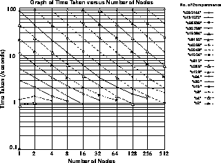
Figure 7.14:
Results from Running a GENESIS Simulation of a Passive Cable
Model Composed of Varying Numbers of Compartments Distributed Across
Varying Numbers of Nodes on the Intel Touchstone Delta Parallel
Supercomputer
The previous record for the most complex GENESIS model produced on a
traditional serial computer is approximately 80,000 elements, the
Purkinje Cell
model produced at Caltech by
Dr. de Schutter [Schutter:91a;93a].
Using the postmaster
element on a parallel supercomputer (the 512-node Intel Touchstone
Delta), this limit has now been pushed to over two million GENESIS
elements (actually  ). As can be seen, this now
allows for the construction of far more complex and realistic models
than was previously possible. The present price to be paid for this
freedom is the decision to make the modeller explicitly distribute his
simulation over the available hardware. This was a design decision that
has allowed far greater efficiency of load balancing than would be
possible using an automatic distribution technique as the illustrated
scaling graphs confirm. This technique also has the advantage of
leaving the basic GENESIS script interface unaltered and is applicable
to a wide variety of parallel hardware. As a result of the requirement
to retain compatibility with the existing serial GENESIS implementation,
another benefit has become obvious. By changing only the network layer
of the postmaster element, it is possible to produce a version of the
postmaster that can use traditional serial machines distributed across
the Internet to produce a distributed model, which ties together
existing supercomputers based anywhere on the network. The potential
size of model that can be constructed in this manner is staggering,
although the reality of network communication delays will limit its area
of application to compute-limited tasks (cf. communication-bound
simulations).
). As can be seen, this now
allows for the construction of far more complex and realistic models
than was previously possible. The present price to be paid for this
freedom is the decision to make the modeller explicitly distribute his
simulation over the available hardware. This was a design decision that
has allowed far greater efficiency of load balancing than would be
possible using an automatic distribution technique as the illustrated
scaling graphs confirm. This technique also has the advantage of
leaving the basic GENESIS script interface unaltered and is applicable
to a wide variety of parallel hardware. As a result of the requirement
to retain compatibility with the existing serial GENESIS implementation,
another benefit has become obvious. By changing only the network layer
of the postmaster element, it is possible to produce a version of the
postmaster that can use traditional serial machines distributed across
the Internet to produce a distributed model, which ties together
existing supercomputers based anywhere on the network. The potential
size of model that can be constructed in this manner is staggering,
although the reality of network communication delays will limit its area
of application to compute-limited tasks (cf. communication-bound
simulations).
The assessment of the usefulness of a parallel neural modelling
platform can be demonstrated by two extremes of neural modelling
applications:
-
Detailed single-cell models
The individual subcompartments which make up a neuron's dendritic
tree are active simultaneously, and each of these compartments may be
studded with several independently functioning ionic membrane channels.
This is illustrated in Figure 7.15.
Figure 7.15:
Cerebella Purkinle cell model in GENESIS.
Our most detailed single-cell model to date.
-
Large network simulations
A detailed network simulation may be composed of many thousands of
individual nerve cells from a smaller number of biological cell types.
What does a parallel computer have to offer the single-cell modeller?
Most of the work on the parallel GENESIS at Caltech to date has been in
the field of single-cell modelling. Several distinct ways of using the
system have been developed allowing a variety of approaches by the
single-cell modeller.
-
Examining large parameter spaces
Each individual node on the parallel computer runs a separate, complete,
single-cell model (task farming). This facility can be used to examine
the sensitivity of the cell's performance to a wide range of
physiological states including testing the effect of parameters which
are at present difficult to measure experimentally [
Bhalla:93a
]. A
selection of these appear below:
-
-
-
Channel Blocker Experiments.
Like the experimentalist, the neural modeller can block or poison
different ion channel subsets, with the added advantage that it is
possible to block both channels where no chemical
blocking
agent currently exists and also to have 100%
channel-blocking
specificity (e.g., work conducted by
D. Jaeger, Caltech [
Jaeger:93a
]).
-
-
-
Effect of stimulation in different parts of the dendritic arbor
An experiment at present difficult or impossible to perform in any
physiological setup can easily be tested on the computer model system.
For example, the independence of stimulation site on Purkinje Cell
response (Work performed by E. de Schutter, Caltech [Schutter:91a;93a]).
-
-
-
Prediction of ionic channel distribution
The prediction of ionic channel distribution over different parts of a
cell's dendritic arbor by observing the effect of changed distribution
on the model cell's electrophysiological properties, and relating this
to the experimentally measured behavior of the real neuron
[
Bhalla:93a
]. Experimental confirmation of channel distribution
predicted by the manipulation of such computer models seems likely to
appear in the near future due to advances in monoclonal antibody
techniques for different channel subsets.
-
-
-
Effect of changing membrane properties
Predicting the effect of changing membrane properties which are
impossible to measure experimentally-for example, in the distal
dendritic arbor or in ``spines'' (e.g., E. de Schutter, Caltech
[
Bhalla:93a
], [
Schutter:91a
]).
The first example above is of modelling following and confirming
physiology experiments. The latter examples are uses of neural
modelling to predict future experimental findings. Although rarely
used to date (because of computer limits on the model's level of
biological realism), this synergistic use of neural modelling in
predicting experimental results and suggesting new experiments appears
to offer substantial benefits to the neurobiology community at large.
Neural modelling on parallel computers, such as the Intel Touchstone
Delta, is allowing modelling to adopt these new closer links to
experimental work, thereby closing the dichotomy between experimenters
and modellers. In the past, this dichotomy has caused several
experimentalists to question the relevance of funding modelling work.
Hopefully, this attitude will change as more results of synergy between
modelling experiments and physiology experiments become widely known.
-
Construction of large and detailed cell models
The system allows the construction of larger and more detailed cell
models than is possible on a traditional serial computer. The level of
detail included in models to date has been limited either by the memory
size constraints of the computer used, or by the computational time
requirements of the model [
Bhalla:92a
]. A distributed model of a
single cell on a parallel computer alleviates both of these constraints
simultaneously. This allows the construction of larger cell models than
have been previously possible but which nevertheless run in acceptable
time frames.
What does a parallel computer have to offer the neural network
modeller?
Much of the work to date has been on task farming (as described above),
whereby each node runs its own copy of a cell. This is less useful to
the network modeller but still allows detailed statistical information
to be built up about network and population behavior. A more
interesting way of using the parallel machine for network modelling is
the distributed model scheme mentioned above. This allows networks to
be both larger and to run more quickly than their counterparts on
equivalent serial machines. A promising project in this category,
although still in its very early stages, is the construction by
Upinder Bhalla at Caltech of a detailed model of the rat olfactory bulb
[
Bhalla:93a
]. This incorporates detailed cellular
elements, which are rare in network class models. Such a
network model makes far greater communication demands of the internode
communications mechanism on the parallel computer than a distributed
single-cell model. Initially an expanded version of the postmaster
element [Speight:92a;92b]
which was used for distributed single-cell models will be employed, but
this may change as the different demands of a large network model
become apparent.
All of the work on the Parallel GENESIS project was carried out in the
laboratory of Professor James Bower at the California Institute of
Technology.
Next:
Full Matrix Algorithms
Up:
Parallel Computing in
Previous:
7.6.5 Task Farming
Guy Robinson
Wed Mar 1 10:19:35 EST 1995
Full Matrix Algorithms and Their
Applications
Next:
8.1 Full and Banded
Up:
Parallel Computing Works
Previous:
7.6.6 Distributed Modelling via
Guy Robinson
Wed Mar 1 10:19:35 EST 1995
8.1 Full and Banded Matrix Algorithms
Next:
8.1.1 Matrix Decomposition
Up:
Full Matrix Algorithms
Previous:
Full Matrix Algorithms
Concurrent matrix algorithms
were among the
first to be studied on the hypercubes at Caltech [
Fox:82a
], and
they have also been intensively studied at other institutions, notably
Yale [
Ipsen:87b
], [Johnsson:87b;89a],
[
Saad:85a
], and Oak Ridge National
Laboratory [Geist:86a;89a], [Romine:87a;90a].
The
motivation for this interest is the fact that matrix algorithms play a
prominent role in many scientific and engineering computations. In
this chapter, we study the so called-
full
or
dense
(and
closely related
banded
) matrix
algorithms
where essentially all elements of the matrix are nonzero. In
Chapters
9
and
12
, we will treat the more common case
of problems, which, if formulated as matrix equations, are represented
by
sparse
matrices. Here, most of the elements of the matrix
are zero; one can apply full matrix algorithms to such sparse cases,
but there are much better algorithms that exploit the sparseness to
reduce the computational complexity. Within C P, we found two
classes of important problems that needed full matrix algorithms. In
Sections
8.2
and
8.3
, we cover two chemical scattering
problems, which involve relatively small full matrices-where the
matrix rows and columns are labelled by the different reaction
channels. The currently most important real-world use of full matrix
algorithms is computational electromagnetic
simulations
[
Edelman:92a
]. These are used by the defense industry to design
aircraft and other military vehicles with low radar cross sections.
Solutions of large sets of linear equations come from the method of
moments approach to electromagnetic equations [
Wang:91b
]. We
investigated this method successfully at JPL [
Simoni:89a
] but in
this book, we only describe (in Section
9.4
) the alternative
approaches, finite elements, to electromagnetic simulations. Such
sparse matrix
formulation will be more efficient
for large electromagnetic problems, but the moment method and
associated full matrix is probably the most common and numerically
reliable approach.
P, we found two
classes of important problems that needed full matrix algorithms. In
Sections
8.2
and
8.3
, we cover two chemical scattering
problems, which involve relatively small full matrices-where the
matrix rows and columns are labelled by the different reaction
channels. The currently most important real-world use of full matrix
algorithms is computational electromagnetic
simulations
[
Edelman:92a
]. These are used by the defense industry to design
aircraft and other military vehicles with low radar cross sections.
Solutions of large sets of linear equations come from the method of
moments approach to electromagnetic equations [
Wang:91b
]. We
investigated this method successfully at JPL [
Simoni:89a
] but in
this book, we only describe (in Section
9.4
) the alternative
approaches, finite elements, to electromagnetic simulations. Such
sparse matrix
formulation will be more efficient
for large electromagnetic problems, but the moment method and
associated full matrix is probably the most common and numerically
reliable approach.
Early work at Caltech on full matrices (1983 to 1987) focused on specific
algorithms, such as matrix multiplication, matrix-vector products, and
LU decomposition.
A major issue
in determining the optimal algorithm for these problems is choosing a
decomposition which has good load balance and low communication
overhead. Many matrix algorithms proceed in a series of steps in which
rows and/or columns are successively made inactive. The scattered
decomposition
described in
Section
8.1.2
is usually used to balance the load in such
cases. The block decomposition, also described in
Section
8.1.2
, generally minimizes the amount of data
communicated, but results in sending several short messages rather than
a few longer messages. Thus, a block decomposition is optimal for a
multiprocessor with low message latency,
or startup
cost, such as the Caltech/JPL Mark II hypercube. For machines with
high message latency, such as the Intel iPSC/1, a row decomposition may
be preferable. The best decomposition, therefore, depends crucially on
the characteristics of the concurrent hardware.
In recent years (1988-1990), interest has centered on the development of
libraries of concurrent linear algebra routines. As discussed in
Section
8.1.7
, two approaches have been followed at Caltech. One
approach by Fox, et al. has led to a library of routines that are
optimal for low latency, homogeneous hypercubes, such as the Caltech/JPL
Mark II hypercubes. In contrast, Van de Velde has developed a library of
routines that are generally suboptimal, but which may be ported to a wider
range of multiprocessor architectures, and are suitable for incorporation into
programs with dynamically changing data distributions.
Other References
HPFA Applications and Paradigms
Next:
8.1.1 Matrix Decomposition
Up:
Full Matrix Algorithms
Previous:
Full Matrix Algorithms
Guy Robinson
Wed Mar 1 10:19:35 EST 1995
8.1.1 Matrix Decomposition
Next:
8.1.2 Basic Matrix Arithmetic
Up:
8.1 Full and Banded
Previous:
8.1 Full and Banded
The data decomposition (or distribution) is a major factor in determining the
efficiency of a concurrent matrix algorithm, so before
detailing the research into concurrent linear algebra done at Caltech, we
shall first introduce some basic decomposition strategies.
The processors of a concurrent computer can be uniquely labelled by
 , where
  is the number of
processors. A vector of length
M
may be decomposed over the
processors by assigning the vector entry with global index
m
(where
is the number of
processors. A vector of length
M
may be decomposed over the
processors by assigning the vector entry with global index
m
(where
 ) to processor
p
, where it is stored as the
i
entry
in a local array. Thus, the decomposition of a vector can be regarded
as a mapping of the global index,
m
, to an index pair,
) to processor
p
, where it is stored as the
i
entry
in a local array. Thus, the decomposition of a vector can be regarded
as a mapping of the global index,
m
, to an index pair,  ,
specifying the processor number and local index.
,
specifying the processor number and local index.
For matrix problems, the processors are usually arranged as a  grid. Thus, the grid consists of
P
rows of processors and
Q
columns of processors, and
grid. Thus, the grid consists of
P
rows of processors and
Q
columns of processors, and  . Each processor can be uniquely
identified by its position,
. Each processor can be uniquely
identified by its position,  , on the processor grid. The
decomposition of an
, on the processor grid. The
decomposition of an  matrix can be regarded as the
Cartesian
product of two vector decompositions,
matrix can be regarded as the
Cartesian
product of two vector decompositions,  and
and  . The mapping
  decomposes the
M
rows of the matrix
over the
P
processor rows, and
decomposes the
M
rows of the matrix
over the
P
processor rows, and  decomposes the
N
columns of
the matrix over the
Q
processor columns. Thus, if
decomposes the
N
columns of
the matrix over the
Q
processor columns. Thus, if  and
and
 , then the matrix entry with global index
  is
assigned to the processor at position
is
assigned to the processor at position  on the processor grid,
where it is stored in a local array with index
on the processor grid,
where it is stored in a local array with index  .
.
Two common decompositions are the
linear
and
scattered
decompositions. The linear decomposition,  , assigns
contiguous entries in the global vector to the processors in blocks,
, assigns
contiguous entries in the global vector to the processors in blocks,

where

and  and
and  . The scattered decomposition,
 , assigns consecutive entries in the global vector to different
processors,
, assigns consecutive entries in the global vector to different
processors,

Figure
8.1
shows examples of these two types of decomposition
for a  matrix.
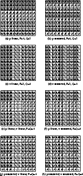
Figure 8.1:
These Eight Figures Show Different Ways of Decomposing a
 Matrix. Each cell represents a matrix entry, and is
labelled by the position,
Matrix. Each cell represents a matrix entry, and is
labelled by the position,  , in the processor grid of the
processor to which it is assigned. To emphasize the pattern of
decomposition, the matrix entries assigned to the processor in the
first row and column of the processor grid are shown shaded. Figures
(a) and (b) show linear and scattered row-oriented decompositions,
respectively, for four processors arranged as a
, in the processor grid of the
processor to which it is assigned. To emphasize the pattern of
decomposition, the matrix entries assigned to the processor in the
first row and column of the processor grid are shown shaded. Figures
(a) and (b) show linear and scattered row-oriented decompositions,
respectively, for four processors arranged as a  grid
(
P=4
,
Q=1
). In Figures (c) and (d), the corresponding
column-oriented decompositions are shown (
P=1
,
Q=4
). Figures (e)
through (h) show linear and scattered block-oriented decompositions for
16 processors arranged as a
grid
(
P=4
,
Q=1
). In Figures (c) and (d), the corresponding
column-oriented decompositions are shown (
P=1
,
Q=4
). Figures (e)
through (h) show linear and scattered block-oriented decompositions for
16 processors arranged as a  grid (
P=Q=4
).
grid (
P=Q=4
).
The mapping of processors onto the processor grid is determined by the
programming methodology, which in turn depends closely on the concurrent
hardware. For machines such as the nCUBE-1
hypercube, it
is advantageous to exploit any locality properties in the algorithm in
order to reduce communication costs. In such cases, processors may be
mapped onto the processor grid by a binary Gray code scheme
[
Fox:88a
], [
Saad:88a
], which ensures that adjacent processors
on the processor grid are directly connected by a communication
channel. For machines such as the Symult 2010, for which the time to
send a message between any two processors is almost independent of
their separation in the hardware topology, locality of communication is
not an issue, and the processors can be mapped arbitrarily onto the
processor grid.
Next:
8.1.2 Basic Matrix Arithmetic
Up:
8.1 Full and Banded
Previous:
8.1 Full and Banded
Guy Robinson
Wed Mar 1 10:19:35 EST 1995
8.1.2 Basic Matrix Arithmetic
Next:
8.1.3 Matrix Multiplication for
Up:
8.1 Full and Banded
Previous:
8.1.1 Matrix Decomposition
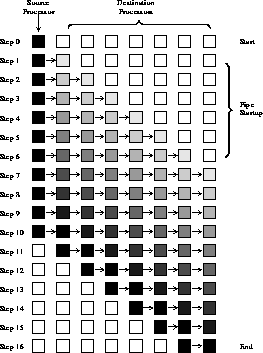
Figure 8.2:
A Schematic Representation of a Pipeline
Broadcast
for an Eight-Processor Computer. White
squares represent processors not involved in communication, and such
processors are available to perform calculations. Shaded squares
represent processors involved in communication, with the degree of
shading indicating how much of the data have arrived at any given
step. In the first six steps, those processor not yet involved in the
broadcast
can continue to perform calculations.
Similarly, in steps 11 through 16, processors that are no longer involved in
communicating can perform useful work since they now have all the data
necessary to perform the next stage of the algorithm.
One of the first linear algebra algorithms implemented on the
Caltech/JPL Mark II hypercube was the multiplication of two dense
matrices,  and
and  , to form the product,
  [
Fox:85b
]. The algorithm uses a block-oriented, linear
decomposition, which is optimal for machines with low message latency
when the subblocks are (as nearly as possible) square. Let us denote
by
[
Fox:85b
]. The algorithm uses a block-oriented, linear
decomposition, which is optimal for machines with low message latency
when the subblocks are (as nearly as possible) square. Let us denote
by  the subblock of
  in the processor at position
 of the processor grid, with a similar designation applying to
the subblocks of
of the processor grid, with a similar designation applying to
the subblocks of  and
and  . Then, if the processor grid is
square, that is,
. Then, if the processor grid is
square, that is,  , the matrix multiplication algorithm
in block form is,
, the matrix multiplication algorithm
in block form is,

The case in which  involves some extra bookkeeping, but does not
change the concurrent algorithm in any essential way.
involves some extra bookkeeping, but does not
change the concurrent algorithm in any essential way.
On the Mark II hypercube, communication cost increases with processor
separation, so processors are mapped onto the processor grid using a
binary Gray code scheme. Two types of communication are required at
each stage of the algorithm, and both exploit the hypercube topology to
minimize communication costs. Matrix subblocks are communicated to the
processor above in the processor grid, and subblocks are
broadcast
along processor rows by a communication
pipeline (Figure
8.2
).
The matrix multiplication algorithm has been modified for use on the
Caltech/JPL Mark IIIfp hypercube [
Hipes:89b
]. The Mark II
hypercube is a homogeneous machine in the sense that there is only one
level in the memory hierarchy, that is, the local memory of each
processor. However, each processor of the Mark IIIfp hypercube has a
Weitek floating-point processor with a  data cache. To
take full advantage of the high processing speed of the Weitek, data
transfer between local memory and the Weitek data cache must be
minimized. Since there are two levels in the memory hierarchy of each
processor (local memory and cache), the Mark IIIfp is an inhomogeneous
hypercube. The main computational task in each stage of the concurrent
algorithm is to multiply the subblocks in each processor, and for large
problems not all of the data will fit into the cache. The
multiplication is, therefore, done in inner product form on the Weitek
by further subdividing the subblocks in each processor. This
intraprocessor subblocking
allows the multiplication in
each processor to be done in a number of stages, during each of which
only the data needed for that stage are explicitly loaded into the
cache.
data cache. To
take full advantage of the high processing speed of the Weitek, data
transfer between local memory and the Weitek data cache must be
minimized. Since there are two levels in the memory hierarchy of each
processor (local memory and cache), the Mark IIIfp is an inhomogeneous
hypercube. The main computational task in each stage of the concurrent
algorithm is to multiply the subblocks in each processor, and for large
problems not all of the data will fit into the cache. The
multiplication is, therefore, done in inner product form on the Weitek
by further subdividing the subblocks in each processor. This
intraprocessor subblocking
allows the multiplication in
each processor to be done in a number of stages, during each of which
only the data needed for that stage are explicitly loaded into the
cache.
Independently, Cherkassky, et al. in [
Cherkassky:88a
], Berntsen
in [
Berntsen:89a
], and Aboelaze [
Aboelaze:89a
] improved
Fox's algorithm for dense  matrix multiplication, reducing the time
complexity from
matrix multiplication, reducing the time
complexity from

to

where  is the number of processors,
  is the time for one
addition or one multiplication, and
is the time for one
addition or one multiplication, and  ,
,  are
machine-dependent communication parameters defining bandwidth and
latency [
Chrisochoides:92a
]. In fact, the communication cost of
transferring
w
words is
are
machine-dependent communication parameters defining bandwidth and
latency [
Chrisochoides:92a
]. In fact, the communication cost of
transferring
w
words is 
A concurrent algorithm to perform the matrix-vector product  has also been implemented on the Caltech/JPL Mark II hypercube
[
Fox:88a
]. Again, a block-oriented, linear decomposition is used for
the matrix
A
. The vector
x
is decomposed linearly over the
processors' columns, so that all the processors in the same processor column
contain the same portion of
x
. Similarly, at the end of the algorithm,
the vector
y
is decomposed over the processor rows, so that all the
processors in the same processor row contain the same portion of
y
. In
block form the matrix-vector product is,
has also been implemented on the Caltech/JPL Mark II hypercube
[
Fox:88a
]. Again, a block-oriented, linear decomposition is used for
the matrix
A
. The vector
x
is decomposed linearly over the
processors' columns, so that all the processors in the same processor column
contain the same portion of
x
. Similarly, at the end of the algorithm,
the vector
y
is decomposed over the processor rows, so that all the
processors in the same processor row contain the same portion of
y
. In
block form the matrix-vector product is,

As in the matrix multiplication algorithm, the concurrent matrix-vector
product algorithm is optimal for low latency, homogeneous hypercubes if the
subblocks of  are square.
Next:
8.1.3 Matrix Multiplication for
Up:
8.1 Full and Banded
Previous:
8.1.1 Matrix Decomposition
Guy Robinson
Wed Mar 1 10:19:35 EST 1995
8.1.3 Matrix Multiplication for Banded Matrices
Next:
8.1.4 Systems of Linear
Up:
8.1 Full and Banded
Previous:
8.1.2 Basic Matrix Arithmetic
Banded Matrix-Vector Multiplication
First, we consider the parallelization of the operation  on a linear array of
  processors when
  is a banded
  matrix with
  ,
,
 upper and lower bandwidths, and we assume that matrices are
stored using a sparse scheme [
Rice:85a
]. For simplicity, we
describe the case
upper and lower bandwidths, and we assume that matrices are
stored using a sparse scheme [
Rice:85a
]. For simplicity, we
describe the case  . The proposed implementation is
based on a decomposition of matrix
. The proposed implementation is
based on a decomposition of matrix  into an upper
  (including the diagonal of
  ) and lower
  triangular
matrices, such as
triangular
matrices, such as  . Furthermore, we
assume that row
. Furthermore, we
assume that row  and
and  are stored
in processor
i
. Without loss of generality, we can assume
are stored
in processor
i
. Without loss of generality, we can assume  and
and  . The vector
  can then be expressed as
 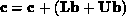 . The products
  and
and  are computed within
  and
and  iterations, respectively.
The computation involved is described in Figure
8.3
. In
order to compute the complexity of the above algorithm, we assume
without any loss of generality, that
iterations, respectively.
The computation involved is described in Figure
8.3
. In
order to compute the complexity of the above algorithm, we assume
without any loss of generality, that  has
K
non-zero elements,
and
has
K
non-zero elements,
and  . Then it can be shown that the time complexity is

and the memory space required for each subdomain is  .
.
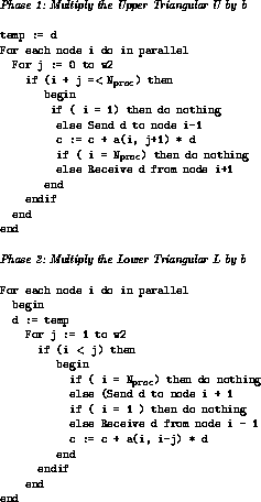
Figure 8.3:
The Pseudo Code for Banded Matrix-Vector Multiplication
Banded Matrix-Matrix Multiplication
Second, we consider the implementation of  , on a ring of
  processors when
 ,
,  are banded
  matrices with
  upper,
and
upper,
and  lower bandwidths, respectively. Again, we describe the
realization for
lower bandwidths, respectively. Again, we describe the
realization for  . The case
  is
straightforward generalization. The processor
i
computes column
is
straightforward generalization. The processor
i
computes column
 of matrix
  and holds one row of matrix
  (denoted by
 ) and a column of matrix
  (denoted by
  ).
).
The algorithm consists of two phases as in banded-matrix vector
multiplication. Without loss of generality, we can assume  , and
, and  . In the first phase, each node starts by
calculating
. In the first phase, each node starts by
calculating  , then each node
i
passes
, then each node
i
passes  to node
i-1
, this phase is repeated
to node
i-1
, this phase is repeated 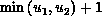 times. In the second phase, each node restores
 and passes it to node
i+1
. This phase is repeated
and passes it to node
i+1
. This phase is repeated  times. The implementation proposed for this operation is
described in Figure
8.4
.
times. The implementation proposed for this operation is
described in Figure
8.4
.
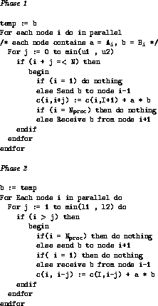
Figure 8.4:
The Pseudo Code for Banded Matrix-Matrix Multiplication
Without loss of generality, we assume that  are the number
of non-zero elements for the matrices
are the number
of non-zero elements for the matrices  ,
,  respectively,
and denote by
respectively,
and denote by  and
and  . Then
we can show that the parallel execution time
. Then
we can show that the parallel execution time  is given by
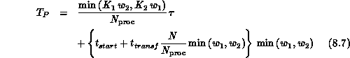
The above realization has been implemented on the nCUBE-1
[
Chrisochoides:90a
]. Tables
8.1
and
8.2
indicate
the performance of BLAS 2
computation
for a block tridiagonal matrix where each block is dense. In these
experiments, each processor has the same computation to perform. The
results indicate very satisfactory performance for these type of data.
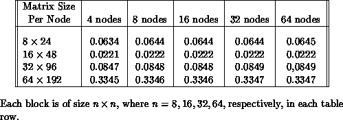
Table 8.1:
Measured maximum total elapsed time (in seconds) for
multiplication of a block tridiagonal matrices with a vector.
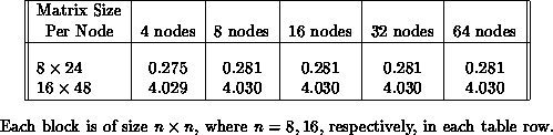
Table 8.2:
Measured maximum elapsed time (in seconds) for multiplication
of a block tridiagonal matrix by a block tridiagonal matrix.
Next:
8.1.4 Systems of Linear
Up:
8.1 Full and Banded
Previous:
8.1.2 Basic Matrix Arithmetic
Guy Robinson
Wed Mar 1 10:19:35 EST 1995
8.1.4 Systems of Linear Equations
Next:
8.1.5 The Gauss-Jordan Method
Up:
8.1 Full and Banded
Previous:
8.1.3 Matrix Multiplication for
Factorization of Full Matrices
LU factorization
of
dense matrices, and the closely related Gaussian
elimination
algorithm, are widely used in
the solution of linear systems of equations of the form  . LU factorization expresses the coefficient matrix,
A
, as the
product of a lower triangular matrix,
L
, and an upper triangular
matrix,
U
. After factorization, the original system of equations can
be written as a pair of triangular systems,
. LU factorization expresses the coefficient matrix,
A
, as the
product of a lower triangular matrix,
L
, and an upper triangular
matrix,
U
. After factorization, the original system of equations can
be written as a pair of triangular systems,

The first of the systems can be solved by forward reduction,
and then back substitution can be used to solve the second
system to give
x
. If
A
is an  matrix, LU
factorization proceeds in
M-1
steps, in the
k
of which column
k
of
L
and row
k
of
U
are found,
matrix, LU
factorization proceeds in
M-1
steps, in the
k
of which column
k
of
L
and row
k
of
U
are found,

and the entries of
A
in a ``window'' extending from column
k+1
to
M-1
and row
k+1
to
M-1
are updated,

Partial pivoting
is usually performed to improve
numerical stability. This involves reordering the rows or columns of
A
.
In the absence of pivoting, the row- and column-oriented decompositions
involve almost the same amounts of communication and computation.
However, the row-oriented approach is generally preferred as it is more
convenient for the back substitution phase [
Chu:87a
],
[
Geist:86a
], although column-based algorithms have been proposed
[
Li:87a
], [
Moler:86a
]. A block-oriented decomposition
minimizes the amount of data communicated, and is the best approach on
hypercubes with low message latency. However, since the block
decomposition generally involves sending shorter messages, it is not
suitable for machines with high message latency. In all cases,
pipelining is the most efficient way of broadcasting
rows and columns of the matrix since it minimizes the idle time that a
processor must wait when participating in a broadcast
,
and effectively overlaps communication and calculation.
Load balance
is an important issue in LU
factorization. If a linear decomposition is used, the computation will
be imbalanced and processors will become idle once they no longer
contain matrix entries in the computational window. A scattered
decomposition
is much more effective in
keeping all the processors busy, as shown in Figure
8.5
.
The load imbalance is least when a scattered block-oriented
decomposition is used.
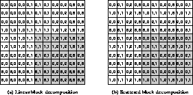
Figure 8.5:
The Shaded Area in These Two Figures Shows the Computational Window
at the Start of Step Three of the LU Factorization Algorithm. In (a) we see
that by this stage the processors in the first row and column of the processor
grid have become idle if a linear block decomposition is used. In contrast,
in (b) we see that all processors continue to be involved in the computation
if a scattered block decomposition is used.
At Caltech, Van de Velde has investigated LU factorization of full matrices
for a number of different pivoting strategies, and for various types of
matrix decomposition on the Intel iPSC/2 hypercube and the Symult 2010
[
Velde:90a
]. One observation based on this work was that if a linear
decomposition is used, then in many cases pivoting results in a faster
algorithm than with no pivoting, since the exchange of rows effectively
randomizes the decomposition, resulting in better load balance. Van de Velde
also introduces a clever enhancement to the standard concurrent partial
pivoting procedure. To illustrate this, consider partial pivoting over rows.
Usually, only the processors in a single-processor column are involved in the
search for the pivot candidate, and the other processors are idle at this
time. In Van de Velde's multirow pivoting scheme, in each processor column a
search for a pivot is conducted concurrently within a randomly selected
column of the matrix. This incurs no extra cost compared with the standard
pivoting procedure, but improves the numerical stability. A similar
multicolumn pivoting scheme can be used when pivoting over columns.
Van de Velde concludes from his extensive experimentation with LU
factorization schemes that a scattered decomposition generally results in a
more efficient algorithm on the iPSC/2 and Symult 2010, and his work
illustrates the importance of decomposition and pivoting strategy in
determining load balance, and hence concurrent efficiency.
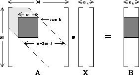
Figure 8.6:
Schematic Representation of Step
k
of LU Factorization for
an  Matrix,
A
, with Bandwidth
w
. The
Matrix,
A
, with Bandwidth
w
. The
 computational window is shown as a dark-shaded square, and
matrix entries in this region are updated at step
k
. The
light-shaded part of the band above and to the left of the window has
already been factorized, and in an in-place algorithm contains the
appropriate columns and rows of
L
and
U
. The unshaded part of the
band below and to the right of the window has not yet been modified.
The shaded region of the matrix
B
represents the
computational window is shown as a dark-shaded square, and
matrix entries in this region are updated at step
k
. The
light-shaded part of the band above and to the left of the window has
already been factorized, and in an in-place algorithm contains the
appropriate columns and rows of
L
and
U
. The unshaded part of the
band below and to the right of the window has not yet been modified.
The shaded region of the matrix
B
represents the  window
updated in step
k
of forward reduction,
and in
step
M-k-1
of back substitution.
window
updated in step
k
of forward reduction,
and in
step
M-k-1
of back substitution.
LU Factorization of Banded Matrices
Aldcroft, et al. [
Aldcroft:88a
] have investigated the
solution of linear systems of equations by LU factorization, followed
by forward elimination and back substitution, when the coefficient
matrix,
A
, is an  matrix of bandwidth
w=2m-1
. The case of multiple right-hand sides was considered, so the
system may be written as
AX=B
, where
X
and
B
are
matrix of bandwidth
w=2m-1
. The case of multiple right-hand sides was considered, so the
system may be written as
AX=B
, where
X
and
B
are  matrices. The LU factorization algorithm for banded matrices is
essentially the same as that for full matrices, except that the
computational window containing the entries of
A
updated in each step
is different. If no pivoting is performed, the window is of size
matrices. The LU factorization algorithm for banded matrices is
essentially the same as that for full matrices, except that the
computational window containing the entries of
A
updated in each step
is different. If no pivoting is performed, the window is of size
 and lies along the diagonal, as shown in
Figure
8.6
. If partial pivoting over rows is performed,
then fill-in will occur, and the window may attain a maximum size of
and lies along the diagonal, as shown in
Figure
8.6
. If partial pivoting over rows is performed,
then fill-in will occur, and the window may attain a maximum size of
 . In the work of Aldcroft, et al. the size of the
window was allowed to vary dynamically. This involved some additional
bookkeeping, but is more efficient than working with a fixed window of
the maximum size. Additional complications arise from only storing the
entries of
A
within the band in order to reduce memory usage.
. In the work of Aldcroft, et al. the size of the
window was allowed to vary dynamically. This involved some additional
bookkeeping, but is more efficient than working with a fixed window of
the maximum size. Additional complications arise from only storing the
entries of
A
within the band in order to reduce memory usage.
As in the full matrix case, good load balance is ensured by using a scattered
block decomposition for the matrices. As noted previously, this choice of
decomposition also minimizes communication cost on low latency
multiprocessors, such as the Caltech/JPL Mark II hypercube used in this work,
but may not be optimal for machines in which the message startup cost is
substantial.
A comparison between an analytic performance model and results on the
Caltech/JPL Mark II hypercube shows that the concurrent overhead for the
LU factorization algorithm falls to zero as  , where
 . This is true in both the pivoting
and non-pivoting cases. Thus, the LU factorization algorithm scales well to
larger machines.
. This is true in both the pivoting
and non-pivoting cases. Thus, the LU factorization algorithm scales well to
larger machines.
Next:
8.1.5 The Gauss-Jordan Method
Up:
8.1 Full and Banded
Previous:
8.1.3 Matrix Multiplication for
Guy Robinson
Wed Mar 1 10:19:35 EST 1995
8.1.5 The Gauss-Jordan Method
Next:
8.1.6 Other Matrix Algorithms
Up:
8.1 Full and Banded
Previous:
8.1.4 Systems of Linear
As described for his chemistry
application in
Section
8.2
, Hipes has studied the use of the
Gauss-Jordan
(GJ) algorithm as a means of solving
systems of linear equations [
Hipes:89b
]. On a sequential
computer, LU factorization followed by forward reduction and back
substitution is preferable over GJ for solving linear systems since the
former has a lower operation count. Another apparent drawback of GJ is
that it has generally been believed that the right hand sides must be
available a priori, which in applications requiring the solution for
multiple right-hand sides is a handicap. Hipes' work has shown that
this is not the case, and that a well-written, parallel GJ solver is
significantly more efficient than using LU factorization with
triangular solvers on hypercubes.
As noted by Gerasoulis, et al. [
Gerasoulis:88a
], GJ does not
require the solution of triangular systems. The solution of such systems by
LU factorization features an outer loop of fixed length and two inner loops
of decreasing length, whereas GJ has two outer fixed-length loops and only
one inner loop of decreasing length. GJ is, therefore, intrinsically more
parallel than the LU solver, and its better load balance compensates for its
higher operation count. Hipes has pointed out that the multipliers generated
in the GJ algorithm can be saved where zeros are produced in the coefficient
matrix. The entries in the coefficient matrix are, therefore, overwritten by
the GJ multipliers, and we shall call this the GJ factorization (although
we are not actually expressing the original matrix
A
as the product of two
matrices). It is now apparent that the right-hand side matrix does
not
have to be known in advance, since a solution can be obtained
using the previously computed multipliers. Another factor, noted by Hipes,
favoring the use of the GJ solver on a multiprocessor, is the larger grain
size maintained throughout the GJ factorization and solution phases, and the
lower communication cost in the GJ solution phase.
Hipes has implemented his GJ solver on the Caltech/JPL Mark III and nCUBE-1
hypercubes, and compared the performance with the usual LU solver
[
Hipes:89d
]. In the GJ factorization, a scattered column decomposition
is used, similar to that shown in Figure
8.1
(d). This ensures
good load balance as columns become eliminated in the course of the algorithm.
In the LU factorization, both rows and columns are eliminated so a scattered
block decomposition is used. On both machines, it was found that the GJ
approach is faster for sufficiently many right-hand sides.
Next:
8.1.6 Other Matrix Algorithms
Up:
8.1 Full and Banded
Previous:
8.1.4 Systems of Linear
Guy Robinson
Wed Mar 1 10:19:35 EST 1995
8.1.6 Other Matrix Algorithms
Next:
8.1.7 Concurrent Linear Algebra
Up:
8.1 Full and Banded
Previous:
8.1.5 The Gauss-Jordan Method
Hipes has also compared the Gaussian-Jordan (GJ) and Gaussian
Elimination
(GE)
algorithms for finding the inverse of a matrix [
Hipes:88a
]. This work
was motivated by an application program that integrates a special system of
ordinary differential equations
that arise in chemical dynamics simulations [
Hipes:87a
],
[
Kuppermann:86a
]. The sequential GJ and GE algorithms have the
same operation count for matrix inversion. However, Hipes found the
parallel GJ inversion has a more homogeneous load distribution, and
requires fewer communication calls than GE inversion, and so should
result in a more efficient parallel algorithm. Hipes has compared the
two methods on the Caltech/JPL Mark II hypercube, and as expected found
that GJ inversion algorithm to be the fastest.
Fox and Furmanski have also investigated matrix algorithms at Caltech
[
Furmanski:88b
]. Among the parallel algorithms they discuss is
the power method for finding the largest
eigenvalue,
and corresponding
eigenvector, and a matrix
A
. This starts with an initial guess,
 , at the eigenvector, and then generates subsequent
estimates using
, at the eigenvector, and then generates subsequent
estimates using

As
k
becomes large,  tends to the eigenvalue with the largest
absolute value (except for a possible sign change), and
tends to the eigenvalue with the largest
absolute value (except for a possible sign change), and  tends to
the corresponding eigenvector. Since the main component of the algorithm is
matrix-vector multiplication, it can be done as discussed in
Section
8.1.2
.
tends to
the corresponding eigenvector. Since the main component of the algorithm is
matrix-vector multiplication, it can be done as discussed in
Section
8.1.2
.
A more challenging algorithm to parallelize is the tridiagonalization
of a symmetric matrix by Householder's
method, which involves the application of a series of rotations to the
original matrix. Although the basic operations involved in each
rotation are straightforward (matrix-vector multiplication, scalar
products, and so on), special care must be taken to balance the load.
This is particularly difficult since the symmetry of the matrix
A
means that the basic structure being processed is triangular, and this
is decomposed into a set of local triangular matrices in the individual
processors. Load balance
is optimized by
scattering the rows over the processors, and the algorithm requires
vectors to be broadcast
and transposed.
Next:
8.1.7 Concurrent Linear Algebra
Up:
8.1 Full and Banded
Previous:
8.1.5 The Gauss-Jordan Method
Guy Robinson
Wed Mar 1 10:19:35 EST 1995
8.1.7 Concurrent Linear Algebra Libraries
Next:
8.1.8 Problem Structure
Up:
8.1 Full and Banded
Previous:
8.1.6 Other Matrix Algorithms
Since matrix algorithms
play such an important role
in scientific computing, it is desirable to develop a library of linear
algebra routines for
concurrent multiprocessors. Ideally, these routines should be optimal and
general-purpose, that is, portable to a wide variety of multiprocessors.
Unfortunately, these two objectives are antagonistic, and an algorithm that
is optimal on one machine will often not be optimal on another machine. Even
among hypercubes it is apparent that the optimal decomposition, and hence the
optimal algorithm, depends on the message latency, with a block decomposition
being best for low latency machines, and a row decomposition often being best
for machines with high latency. Another factor to be considered is that
often a matrix algorithm is only part of a larger application code. Thus,
the data decomposition before and after the matrix computation may not be
optimal for the matrix algorithm itself. We are faced with the choice of
either transforming the decomposition before and after the matrix computation
so that the optimal matrix algorithm can be used, or leaving the
decomposition as it is and using a suboptimal matrix algorithm. To
summarize, the main issues that must be addressed are:
-
optimal or general-purpose routines, and
-
optimal algorithms with data transformation, or suboptimal algorithms
with no data transformation.
Two approaches to designing linear algebra libraries have been followed at
Caltech. Fox, Furmanski, and Walker choose optimality as the most important
concern in developing a set of linear algebra routines for low latency,
homogeneous hypercubes, such as the Caltech/JPL Mark II hypercube. These
routines feature the use of the scattered decomposition
to ensure load balance, and to minimize communication
costs. Transformations between decompositions are performed using the
comutil
library of global communication routines
[
Angus:90a
], [
Fox:88h
], [
Furmanski:88b
]. This approach
was mainly dictated by historical factors, rather than being a
considered design decision-the hypercubes used most at Caltech up to
1987 were homogeneous and had low latency.
A different, and probably more useful approach, has been taken at Caltech
by Van de Velde [
Velde:89b
] who opted for general-purpose library
routines. The decomposition currently in use is passed to a routine through
its argument list, so in general the decomposition is not changed and a
suboptimal algorithm is used. The main advantage of this approach is that it
is decomposition-independent and allows portability of code among a wide
variety of multiprocessors. Also, the suboptimality of a routine must be
weighed against the possibly large cost of transforming the data
decomposition, so suboptimality does not necessarily result in a slower
algorithm if the time to change the decomposition is taken into account.
Occasionally, it may be advantageous to change the decomposition, and most
changes of this type are what Van de Velde calls
orthogonal
. In an
orthogonal redistribution of the data, each pair of processors exchanges the
same amount of data. Van de Velde has shown [
Velde:90c
] that any
orthogonal redistribution can be performed by the following sequence of
operations:
Local permutation - Global transposition - Local permutation
A local permutation merely involves reindexing the local data within
individual processors. If we have
P
processors and
P
data items in each
processor, then the global transposition,  , takes the item with local
index
i
in processor
p
and sends it to processor
i
, where it is stored
with local index
p
. Thus,
, takes the item with local
index
i
in processor
p
and sends it to processor
i
, where it is stored
with local index
p
. Thus,

Van de Velde's
transpose
routine is actually a generalization of the
hypercube-specific
index
routine in the comutil library.
Van de Velde has implemented his linear algebra library on the Intel iPSC/2
and the Symult 2010, and has used it in investigations of concurrent LU and
QR factorization
algorithms [
Velde:89b
],
[
Velde:90a
], and in studies of invariant manifolds of dynamical
systems [
Lorenz:89a
], [
Velde:90b
].
A group centered at Oak Ridge National Laboratory and the University
of Tennessee is leading the development of a major new portable
parallel full matrix library called ScaLAPACK [
Choi:92a
],
[
Choi:92b
]. This is built around an elegant formulation of
matrix problems in terms of the so-called level three BLAS,
which are a set of submatrix operations introduced to
support the basic LAPACK library [
Anderson:90c
], [
Dongarra:90a
].
This full matrix
system embodies earlier ideas
from LINPACK and EISPACK and is designed to ensure data locality and
get good performance on shared-memory and vector supercomputers. The
multicomputer ScaLAPACK is built around the scattered block
decomposition described earlier.
Next:
8.1.8 Problem Structure
Up:
8.1 Full and Banded
Previous:
8.1.6 Other Matrix Algorithms
Guy Robinson
Wed Mar 1 10:19:35 EST 1995
8.1.8 Problem Structure
Next:
8.1.9 Conclusions
Up:
8.1 Full and Banded
Previous:
8.1.7 Concurrent Linear Algebra
The basic matrix algorithms appear to fall in the synchronous class in
the language of Section
3.4
. Correspondingly, one would
expect to get good performance on SIMD machines. This is indeed true
for matrix multiplication, but it is hard to get good SIMD performance
on LU factorization and the more complicated matrix algorithms. Here
the algorithm is not fully synchronous. In particular, there are
several operations involving row or column operations. These lead to
two problems. Firstly, the parallelism is reduced from
 (for an
  matrix) to
  -this is
typically a serious problem on SIMD machines, such as the CM-2 or
Maspar
MP-1,2 which are fine grain and require ``massive
parallelism.'' Secondly, the use of pivoting
clearly introduces irregularity into the algorithm, which complicates
the SIMD implementation. For these reasons, most research on matrix
algorithms has concentrated on MIMD multicomputers, such as the
hypercube.
-this is
typically a serious problem on SIMD machines, such as the CM-2 or
Maspar
MP-1,2 which are fine grain and require ``massive
parallelism.'' Secondly, the use of pivoting
clearly introduces irregularity into the algorithm, which complicates
the SIMD implementation. For these reasons, most research on matrix
algorithms has concentrated on MIMD multicomputers, such as the
hypercube.
Guy Robinson
Wed Mar 1 10:19:35 EST 1995
8.1.9 Conclusions
Next:
Quantum Mechanical Reactive
Up:
8.1 Full and Banded
Previous:
8.1.8 Problem Structure
Work on the concurrent Gauss-Jordan algorithm was mostly done by Paul Hipes.
Eric Van de Velde developed the linear algebra library discussed in
Section
8.1.7
, and collaborated with Jens Lorenz in their work on
invariant manifolds. Many of the other current algorithms were devised by
Geoffrey Fox. Wojtek Furmanski and David Walker worked on routines for
transforming decompositions. The implementation of the banded LU solver on
the Caltech/JPL Mark II hypercube was done by Tom Aldcroft, Arturo Cisneros,
and David Walker.
Guy Robinson
Wed Mar 1 10:19:35 EST 1995
Quantum Mechanical Reactive
ScatteringUsing a High-Performance ParallelComputer
Next:
8.2.1 Introduction
Up:
Full Matrix Algorithms
Previous:
8.1.9 Conclusions
Other References
HPFA Applications and Paradigms
Guy Robinson
Wed Mar 1 10:19:35 EST 1995
8.2.1 Introduction
Next:
8.2.2 Methodology
Up:
Quantum Mechanical Reactive
Previous:
Quantum Mechanical Reactive
There is considerable current interest in performing accurate
quantum mechanical, three-dimensional, reactive
scattering cross section calculations. Accurate solutions have, until
recently, proved to be difficult and computationally expensive to
obtain, in large part due to the lack of sufficiently powerful
computers. Prior to the advent of supercomputers, one could only solve
the equations of motion for model systems or for sufficiently light
atom-diatom systems at low energy [Schatz:75a;76a;76b].
As a
result of the current development of efficient methodologies and
increased access to supercomputers, there has been a remarkable surge
of activity in this field. The use of symmetrized hyperspherical
coordinates
[
Kuppermann:75a
] and
of the local hyperspherical surface function formalism
[
Hipes:87a
], [
Kuppermann:86a
], [
Ling:75a
], has proven to
be a successful approach to solving the three-dimensional Schrödinger
equation [Cuccaro:89a;89b],
[
Hipes:87a
], [
Kuppermann:86a
]. However, even for modest
reactive scattering
calculations, the memory
and CPU demands are so great that even CRAY-type
supercomputers will soon be insufficient to sustain progress.
In this section, we show how quantum
mechanical reactive
scattering calculations can be structured so as to use MIMD-type
parallel computer architectures efficiently. We present a concurrent
algorithm for calculating local hyperspherical surface functions (LHSF)
and use a parallelized version [
Hipes:88b
] of Johnson's
logarithmic derivative method [Johnson:73a;77a;79a],
modified
to include the improvements suggested by Manolopoulos
[
Manolopoulos:86a
], for integrating the resulting coupled channel
reactive scattering equations. We compare the results of scattering
calculations on the Caltech/JPL Mark IIIfp 64-processor hypercube for
the  system
J=0,1,2
partial waves on the LSTH [
Liu:73a
],
[
Siegbahn:78a
], [Truhlar:78a;79a],
potential energy surface, with those of
calculations done on a CRAY X-MP/48 and a CRAY-2. Both accuracy and
performance are discussed, and speed estimates are made for the
Mark IIIfp 128-processor hypercube soon to become available and
compared with those of the San Diego Supercomputer Center CRAY Y-MP/864
machine which has recently been put into operation.
system
J=0,1,2
partial waves on the LSTH [
Liu:73a
],
[
Siegbahn:78a
], [Truhlar:78a;79a],
potential energy surface, with those of
calculations done on a CRAY X-MP/48 and a CRAY-2. Both accuracy and
performance are discussed, and speed estimates are made for the
Mark IIIfp 128-processor hypercube soon to become available and
compared with those of the San Diego Supercomputer Center CRAY Y-MP/864
machine which has recently been put into operation.
Next:
8.2.2 Methodology
Up:
Quantum Mechanical Reactive
Previous:
Quantum Mechanical Reactive
Guy Robinson
Wed Mar 1 10:19:35 EST 1995
8.2.2 Methodology
Next:
8.2.3 Parallel Algorithm
Up:
Quantum Mechanical Reactive
Previous:
8.2.1 Introduction
The detailed formulation of reactive scattering based on hyperspherical
coordinates and local variational hyperspherical surface functions (LHSF) is
discussed elsewhere [
Kuppermann:86a
], [
Hipes:87a
],
[
Cuccaro:89a
]. We present a very brief review to facilitate the
explanation of the parallel algorithms.
For a triatomic system, we label the three atoms  ,
,
 and
and  . Let (
 ) be any cyclic
permutation of the indices (
) be any cyclic
permutation of the indices ( ). We define the
 coordinates, the mass-scaled [Delves:59a;62a]
internuclear vector
coordinates, the mass-scaled [Delves:59a;62a]
internuclear vector  from
from  to
to  , and the mass-scaled
position vector
, and the mass-scaled
position vector  of
of  with respect to
the center of mass of
with respect to
the center of mass of  diatom. The symmetrized
hyperspherical coordinates [
Kuppermann:75a
] are the hyper-radius
diatom. The symmetrized
hyperspherical coordinates [
Kuppermann:75a
] are the hyper-radius
 , and a set of five angles
 ,
,  ,
,  ,
,
 and
and  , denoted collectively as
 . The first two of these are in the range
0
to
. The first two of these are in the range
0
to
 and are, respectively,
  and
the angle between
and
the angle between  and
and  . The
angles
. The
angles  ,
,  are the polar angles of
  in a space-fixed frame and
  is the tumbling
angle of the
is the tumbling
angle of the  ,
,  half-plane around
its edge
half-plane around
its edge  . The Hamiltonian
  is
the sum of a radial kinetic energy operator term in
is
the sum of a radial kinetic energy operator term in  , and the
surface Hamiltonian
, and the
surface Hamiltonian  , which contains all differential
operators in
, which contains all differential
operators in  and the electronically adiabatic potential
 . The surface
Hamiltonian
. The surface
Hamiltonian  depends on
  parametrically and is
therefore the ``frozen'' hyperradius part of
parametrically and is
therefore the ``frozen'' hyperradius part of  .
.
The scattering wave function  is labelled by
the total angular momentum
J
, its projection
M
on the
laboratory-fixed
Z
axis, the inversion parity
is labelled by
the total angular momentum
J
, its projection
M
on the
laboratory-fixed
Z
axis, the inversion parity  with respect to
the center of mass of the system, and the irreducible representation
with respect to
the center of mass of the system, and the irreducible representation
 of the permutation group of the system (
 for
for  ) to
which the electronuclear wave function, excluding the nuclear spin part,
belongs [Lepetit:90a;90b]. It can be expanded in terms of the
LHSF
) to
which the electronuclear wave function, excluding the nuclear spin part,
belongs [Lepetit:90a;90b]. It can be expanded in terms of the
LHSF  defined below, and calculated at the values
 of
of  :
:

The index
i
is introduced to permit consideration of a set of many
linearly independent solutions of the Schrödinger equation corresponding to
distinct initial conditions which are needed to obtain the appropriate
scattering matrices.
The LHSF  and
associated energies
and
associated energies  are,
respectively, the eigenfunctions and eigenvalues
of the surface Hamiltonian
are,
respectively, the eigenfunctions and eigenvalues
of the surface Hamiltonian  . They are obtained using
a variational approach [
Cuccaro:89a
]. The variational basis set
consists of products of Wigner rotation matrices
. They are obtained using
a variational approach [
Cuccaro:89a
]. The variational basis set
consists of products of Wigner rotation matrices
 ,
associated Legendre functions of
,
associated Legendre functions of  and functions of
 which depend parametically on
  and are
obtained from the numerical solution of one-dimensional
eigenvalue-eigenfunction differential equations in
and are
obtained from the numerical solution of one-dimensional
eigenvalue-eigenfunction differential equations in  ,
involving a potential related to
,
involving a potential related to
 .
.
The variational method leads to an eigenvalue problem with coefficient and
overlap matrices  and
and
 and whose elements are five-dimensional
integrals involving the variational basis functions.
and whose elements are five-dimensional
integrals involving the variational basis functions.
The coefficients  defined by
Equation
8.12
satisfy a coupled set of second-order
differential equations involving an interaction matrix
defined by
Equation
8.12
satisfy a coupled set of second-order
differential equations involving an interaction matrix
 whose elements are defined
by
whose elements are defined
by
The configuration space  is divided into a set of
Q
hyperspherical shells
is divided into a set of
Q
hyperspherical shells  within each of which we choose a value
  used in
expansion
8.12
.
used in
expansion
8.12
.
When changing from the LHSF set at  to the one at
 , neither
  nor its derivative with
respect to
nor its derivative with
respect to  should change. This imposes continuity conditions on the
 and their
  -derivatives at
  ,
involving the overlap matrix
,
involving the overlap matrix  between the LHSF evaluated at
  and
and


The five-dimensional integrals required to evaluate the elements of
 ,
,  ,
,  , and
, and
 are performed analytically over
  ,
,
 , and
, and  and by two-dimensional numerical
quadratures over
and by two-dimensional numerical
quadratures over  and
and  . These
quadratures account for 90% of the total time needed to calculate the LHSF
. These
quadratures account for 90% of the total time needed to calculate the LHSF
 and the matrices
  and
and
 .
.
The system of second-order ordinary differential equations
in the  is integrated
as an initial value problem from small values of
is integrated
as an initial value problem from small values of  to large values
using Manolopoulos' logarithmic derivative propagator
[
Manolopoulos:86a
]. Matrix inversions account for more than 90%
of the time used by this propagator. All aspects of the physics can be
extracted from the solutions at large
to large values
using Manolopoulos' logarithmic derivative propagator
[
Manolopoulos:86a
]. Matrix inversions account for more than 90%
of the time used by this propagator. All aspects of the physics can be
extracted from the solutions at large  by a constant
  projection [
Hipes:87a
], [
Hood:86a
], [
Kuppermann:86a
].
projection [
Hipes:87a
], [
Hood:86a
], [
Kuppermann:86a
].
Next:
8.2.3 Parallel Algorithm
Up:
Quantum Mechanical Reactive
Previous:
8.2.1 Introduction
Guy Robinson
Wed Mar 1 10:19:35 EST 1995
8.2.3 Parallel Algorithm
Next:
8.2.4 Results and Discussion
Up:
Quantum Mechanical Reactive
Previous:
8.2.2 Methodology
The computer used for this work is a 64-processor Mark IIIfp
hypercube. The Crystalline Operating System (CrOS)-channel-addressed
synchronous communication provides the library routines to handle
communications between nodes
[Fox:85d;85h;88a]. The programs are written in C
programming language except for the time-consuming two-dimensional
quadratures and matrix inversions, which are optimized in assembly
language.
The hypercube was configured as a two-dimensional array of processors.
The mapping is done using binary Gray codes [
Gilbert:58a
],
[
Fox:88a
], [
Salmon:84b
], which gives the
Cartesian
coordinates in processor space and
communication channel tags for a processor's nearest neighbors.
We mapped the matrices into processor space by local decomposition. Let
 and
and  be the number of processors in the rows and columns of the
hypercube configuration, respectively. Element
be the number of processors in the rows and columns of the
hypercube configuration, respectively. Element  of an
of an  matrix is placed in processor row
  and column
  ,
where
,
where  means the integer part of
x
.
means the integer part of
x
.
The parallel code implemented on the hypercube consists of five major steps.
Step one constructs, for each value of  , a primitive basis set
composed of the product of Wigner rotation matrices, associated Legendre
functions, and the numerical one-dimensional functions in
, a primitive basis set
composed of the product of Wigner rotation matrices, associated Legendre
functions, and the numerical one-dimensional functions in  mentioned in Section
8.2.2
and obtained by solving the corresponding
one-dimensional eigenvalue-eigenvector differential equation using a finite
difference method. This requires that a subset of the eigenvalues and
eigenvectors of a tridiagonal matrix be found.
mentioned in Section
8.2.2
and obtained by solving the corresponding
one-dimensional eigenvalue-eigenvector differential equation using a finite
difference method. This requires that a subset of the eigenvalues and
eigenvectors of a tridiagonal matrix be found.
A bisection method [
Fox:84g
], [Ipsen:87a;87c],
which accomplishes the eigenvalue computation using
the TRIDIB routine from EISPACK [
Smith:76a
], was ported to the
Mark IIIfp. This implementation of the bisection method allows
computation of any number of consecutive eigenvalues specified by their
indices. Eigenvectors are obtained using the EISPACK inverse iteration
routine TINVIT with modified Gram-Schmidt orthogonalization. Each
processor solves independent tridiagonal eigenproblems since the number
of eigenvalues desired from each tridiagonal system is small, but there
are a large number of distinct tridiagonal systems. To achieve load
balancing, we distributed subsets of the primitive functions among the
processors in such a way that no processor computes greater than one
eigenvalue and eigenvector more than any other. These large grain
tasks are most easily implemented on MIMD machines; SIMD (Single
Instruction Multiple Data) machines would require more extensive
modifications and would be less efficient because of the sequential
nature of effective eigenvalue iteration
procedures. The one-dimensional bases obtained are then
broadcast
to all the other nodes.
In step two, a large number of two-dimensional quadratures involving the
primitive basis functions which are needed for the variational procedure are
evaluated. These quadratures are highly parallel procedures requiring no
communication overhead once each processor has the necessary subset of
functions. Each processor calculates a subset of integrals independently.
Step three assembles these integrals into the real symmetric dense
matrices  and
and
 which are distributed over
processor space. The entire spectrum of eigenvalues and
eigenvectors
for the associated
variational problem is sought. With the parallel implementation of the
Householder
method [
Fox:84h
],
[
Patterson:86a
], this generalized eigensystem is tridiagonalized
and the resulting single tridiagonal matrix
is solved completely in each processor with the QR
algorithm
[
Wilkinson:71a
]. The QR
implementation is purely sequential since each processor obtains the
entire solution to the eigensystem. However, only different subsets of
the solution are kept in different processors for the evaluation of the
interaction and overlap matrices in step four. This part of the
algorithm is not time consuming and the straightforward sequential
approach was chosen. It has the further effect that the resulting
solutions are fully distributed, so no communication is required.
which are distributed over
processor space. The entire spectrum of eigenvalues and
eigenvectors
for the associated
variational problem is sought. With the parallel implementation of the
Householder
method [
Fox:84h
],
[
Patterson:86a
], this generalized eigensystem is tridiagonalized
and the resulting single tridiagonal matrix
is solved completely in each processor with the QR
algorithm
[
Wilkinson:71a
]. The QR
implementation is purely sequential since each processor obtains the
entire solution to the eigensystem. However, only different subsets of
the solution are kept in different processors for the evaluation of the
interaction and overlap matrices in step four. This part of the
algorithm is not time consuming and the straightforward sequential
approach was chosen. It has the further effect that the resulting
solutions are fully distributed, so no communication is required.
Step four evaluates the two-dimensional quadratures needed for the
interaction  and
overlap
and
overlap  matrices. The same type of algorithms are used as in step two. By
far, the most expensive part of the sequential version of the surface
function calculation is the calculation of the large number of
two-dimensional numerical integrals required by steps two and four.
These steps are, however, highly parallel and well suited for the
hypercube.
matrices. The same type of algorithms are used as in step two. By
far, the most expensive part of the sequential version of the surface
function calculation is the calculation of the large number of
two-dimensional numerical integrals required by steps two and four.
These steps are, however, highly parallel and well suited for the
hypercube.
Step five uses Manolopoulos' [
Manolopoulos:86a
] algorithm to integrate
the coupled linear ordinary differential equations. The parallel
implementation of this algorithm is discussed elsewhere [
Hipes:88b
].
The algorithm is dominated by parallel Gauss-Jordan matrix inversion and is
I/O
intensive, requiring the input of one interaction
matrix per integration step. To reduce the I/O overhead, a second
source of parallelism is exploited. The entire interaction matrix (at
all  ) and overlap matrix (at all
  ) data sets are
loaded across the processors, and many collision energies are
calculated simultaneously. This strategy works because the same set of
data is used for each collision energy, and because enough main memory
is available. Calculation of scattering matrices from the final
logarithmic derivative matrices is not computationally intensive, and
is done sequentially.
) data sets are
loaded across the processors, and many collision energies are
calculated simultaneously. This strategy works because the same set of
data is used for each collision energy, and because enough main memory
is available. Calculation of scattering matrices from the final
logarithmic derivative matrices is not computationally intensive, and
is done sequentially.
The program steps were all run on the Weitek coprocessor, which only supports
32-bit arithmetic. Experimentation has shown that this precision is
sufficient for the work reported below. The 64-bit arithmetic hardware
needed for larger calculations was installed after the present calculations
were completed.
Next:
8.2.4 Results and Discussion
Up:
Quantum Mechanical Reactive
Previous:
8.2.2 Methodology
Guy Robinson
Wed Mar 1 10:19:35 EST 1995
8.2.4 Results and Discussion
Next:
Studies of Electron-Molecule
Up:
Quantum Mechanical Reactive
Previous:
8.2.3 Parallel Algorithm
Accuracy
Calculations were performed for the  system on the LSTH
surface [
Liu:73a
], [
Siegbahn:78a
],
[Truhlar:78a;79a] for partial waves with total
angular momentum
J = 0,1,2
and energies up to
system on the LSTH
surface [
Liu:73a
], [
Siegbahn:78a
],
[Truhlar:78a;79a] for partial waves with total
angular momentum
J = 0,1,2
and energies up to  . Flux is
conserved to better than 1% for
J = 0
, 2.3% for
J = 1
, and 3.6%
for
J = 2
for all open channels over the entire energy range considered.
. Flux is
conserved to better than 1% for
J = 0
, 2.3% for
J = 1
, and 3.6%
for
J = 2
for all open channels over the entire energy range considered.
To illustrate the accuracy of the 32-bit arithmetic calculations, the
scattering results from the Mark IIIfp with 64 processors are shown in
Figure
8.7
for
J = 0
, in which some transition probabilities
as a function of the total collision energy,
E
, are plotted. The
differences between these results, and those obtained using a CRAY X-MP/48
and a CRAY-2, do not exceed 0.004 in absolute value over the energy range
investigated.
Figure 8.7:
Probabilities as a Function of Total Energy
E
(Lower Abscissa)
and Initial Relative Translational Energy  (Upper Abscissa) for the
 Symmetry Transition in
 Collisions on the LSTH Potential Energy Surface. The symbol
 labels an asymptotic state of the
  system in which
v
,
j
, and
system in which
v
,
j
, and  are the quantum numbers of the initial or final
  states. The vertical arrows on the upper abscissa denote the energies at
which the corresponding
states. The vertical arrows on the upper abscissa denote the energies at
which the corresponding  states open up. The length of those
arrows decreases as
v
spans the values 0, 1, and 2, and the numbers 0, 5,
and 10 associated with the arrows define a labelling for the value of
j
.
The number of LHSF used was 36 and the number of primitives used to calculate
these surface functions was 80.
states open up. The length of those
arrows decreases as
v
spans the values 0, 1, and 2, and the numbers 0, 5,
and 10 associated with the arrows define a labelling for the value of
j
.
The number of LHSF used was 36 and the number of primitives used to calculate
these surface functions was 80.
Table 8.3:
Performance of the surface function code.*
Timing and Parallel Efficiency
In Tables
8.3
and
8.4
, we present the
timing data on the 64-processor Mark IIIfp, a CRAY X-MP/48 and a CRAY 2, for
both the surface function code (including calculation of the overlap
 and interaction
  matrices) and the logarithmic derivative propagation code. For the surface
function code, the speeds on the first two machines are about the same.
The CRAY 2 is 1.43 times faster than the Mark IIIfp and 1.51 times faster
than the CRAY X-MP/48 for this code. The reason is that this program is
dominated by matrix-vector multiplications which are done in optimized
assembly code in all three machines. For this particular operation, the
CRAY 2 is 2.03 times faster than the CRAY X-MP/48 whereas, for more
memory-intensive operations, the CRAY 2 is slower than the CRAY X-MP/48
[
Pfeiffer:90a
]. A slightly larger primitive basis set is required on
the Mark IIIfp in order to obtain surface function energies of an accuracy
equivalent to that obtained with the CRAY machines. This is due to the lower
accuracy of the 32-bit arithmetic of the former with respect to the 64-bit
arithmetic of the latter.
matrices) and the logarithmic derivative propagation code. For the surface
function code, the speeds on the first two machines are about the same.
The CRAY 2 is 1.43 times faster than the Mark IIIfp and 1.51 times faster
than the CRAY X-MP/48 for this code. The reason is that this program is
dominated by matrix-vector multiplications which are done in optimized
assembly code in all three machines. For this particular operation, the
CRAY 2 is 2.03 times faster than the CRAY X-MP/48 whereas, for more
memory-intensive operations, the CRAY 2 is slower than the CRAY X-MP/48
[
Pfeiffer:90a
]. A slightly larger primitive basis set is required on
the Mark IIIfp in order to obtain surface function energies of an accuracy
equivalent to that obtained with the CRAY machines. This is due to the lower
accuracy of the 32-bit arithmetic of the former with respect to the 64-bit
arithmetic of the latter.
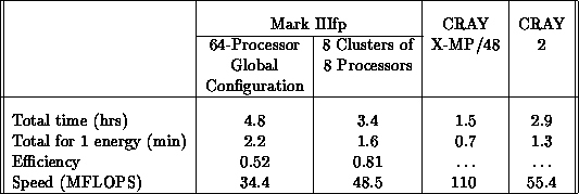
Table 8.4:
Performance of the logarithmic derivative code. Based on a
calculation using 245 surface functions and 131 energies, and a
logarithmic derivative integration step of 0.01 bohr.
The efficiency ( ) of the parallel LHSF code was determined
using the definition
) of the parallel LHSF code was determined
using the definition  , where
 and
and  are, respectively, the implementation times using a
single-processor and
N
processors. The single processor times are
obtained from runs performed after removing the overhead of the
parallel code, that is, after removing the communication calls and some
logical statements. Perfect efficiency (
are, respectively, the implementation times using a
single-processor and
N
processors. The single processor times are
obtained from runs performed after removing the overhead of the
parallel code, that is, after removing the communication calls and some
logical statements. Perfect efficiency ( ) implies
that the
N
-processor hypercube is
N
times faster than a single
processor. In Figure
8.8
, efficiencies for the surface
function code (including the calculation of the overlap and interaction
matrices) as a function of the size of the primitive basis set are
plotted for 2, 4, 8, 16, 32 and 64 processor configurations of the
hypercube. The global dimensions of the matrices used are chosen to be
integer multiples of the number of processor rows and columns in order
to insure load balancing among the processors. Because of the limited
size of a single-processor memory, the efficiency determination is
limited to 32 primitives. As shown in Figure
8.8
, the
efficiencies increase monotonically and approach unity asymptotically
as the size of the calculation increases. Converged results require
large enough primitive basis sets so that the efficiency of the surface
function code is estimated to be about 0.95 or greater.
) implies
that the
N
-processor hypercube is
N
times faster than a single
processor. In Figure
8.8
, efficiencies for the surface
function code (including the calculation of the overlap and interaction
matrices) as a function of the size of the primitive basis set are
plotted for 2, 4, 8, 16, 32 and 64 processor configurations of the
hypercube. The global dimensions of the matrices used are chosen to be
integer multiples of the number of processor rows and columns in order
to insure load balancing among the processors. Because of the limited
size of a single-processor memory, the efficiency determination is
limited to 32 primitives. As shown in Figure
8.8
, the
efficiencies increase monotonically and approach unity asymptotically
as the size of the calculation increases. Converged results require
large enough primitive basis sets so that the efficiency of the surface
function code is estimated to be about 0.95 or greater.
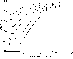
Figure 8.8:
Efficiency of the Surface Function Code (Including the Calculation
of the Overlap and Interaction Matrices) as a Function of the Global Matrix
Dimension (i.e., the Size of the Primitive Basis Set) for 2, 4, 8, 16,
32, and 64 Processors. The solid curves are straight line segments
connecting the data points for a fixed number of processors and are provided
as an aid to examine the trends.
The data for the logarithmic derivative code given in
Table
8.4
for a 245-channel (i.e., LHSF) example show
that the Mark IIIfp has a speed about 62% of that of the CRAY 2, but
only about 31% of that of the CRAY X-MP/48. This code is dominated by
matrix inversions, which are done in optimized assembly code in all
three machines. The reason for the slowness of the hypercube with
respect to the CRAYs is that the efficiency of the parallel logarithmic
derivative code is 0.52. This relatively low value is due to the fact
that matrix inversions require a significant amount of interprocessor
communication. Figure
8.9
displays efficiencies of the
logarithmic derivative code as a function of the number of channels
propagated for different processor configurations, as done previously
for the Mark III [
Hipes:88b
], [
Messina:90a
] hypercubes. The
data can be described well by an operations count formula developed
previously for the matrix inversion part of the code
[
Hipes:88a
]; this formula can be used to extrapolate the data to
larger numbers of processors or channels. It can be seen that for an
8-processor configuration, the code runs with an efficiency of 0.81.
This observation suggested that we divide the Mark IIIfp into eight
clusters of eight processors each, and perform calculations for
different energies in different clusters. The corresponding timing
information is also given in Table
8.4
. As can be seen
from the last row of this table, the speed of the logarithmic
derivative code using this configuration of the 64-processor Mark IIIfp
is  , which is about 44% of that of the CRAY X-MP/48
and 88% of that of the CRAY 2. As the number of channels increases,
the number of processors per cluster may be made larger in order to
increase the amount of memory available in each cluster. The
corresponding efficiency should continue to be adequate due to the
larger matrix dimensions involved.
, which is about 44% of that of the CRAY X-MP/48
and 88% of that of the CRAY 2. As the number of channels increases,
the number of processors per cluster may be made larger in order to
increase the amount of memory available in each cluster. The
corresponding efficiency should continue to be adequate due to the
larger matrix dimensions involved.
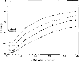
Figure 8.9:
Efficiency of Logarithmic Derivative Code as a Function of the
Global Matrix Dimension (i.e., the Number of Channels or LHSF) for 8,
16, 32, and 64 Processors. The solid curves are straight-line segments
connecting the data points for a fixed number of processors, and are provided
as an aid to examine the trends.
Planned upgrades of the Mark IIIfp include increasing the number of
processors to 128, and replacement of the I/O system will be
high-performance CIO (concurrent I/O) hardware. Further new Weitek
coprocessors, installed since the present calculations were done,
perform 64-bit floating-point arithmetic at about the same nominal peak
speed as the 32-bit boards. From the data in the present paper, it is
possible to predict with good reliability the performance of this
upgraded version of the Mark IIIfp (the CIO upgrade was never
performed). A CRAY Y-MP/864 was installed at the San Diego
Supercomputer Center and measurements show that it is about two times
faster than the CRAY X-MP/48 for the surface function code and 1.7
times faster for the logarithmic derivative code. In
Table
8.5
, we summarize the available or predicted speed
information for the present codes for the current 64-processor and the
planned 128-processor Mark IIIfp, as well as the CRAY X-MP/48, CRAY 2,
and CRAY Y-MP/864 supercomputers. It can be seen that Mark IIIfp
machines are competitive with all of the currently available CRAYs
(operating as single-processor machines). The results described in
this paper demonstrate the feasibility of performing reactive
scattering
calculations with high efficiency
in parallel fashion. As the number of processors continues to
increase, such parallel calculations in systems of greater complexity
will become practical in the not-too-distant future.
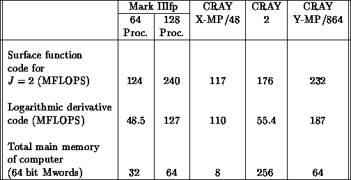
Table 8.5:
Overall speed of reactive scattering codes on several machines.
Next:
Studies of Electron-Molecule
Up:
Quantum Mechanical Reactive
Previous:
8.2.3 Parallel Algorithm
Guy Robinson
Wed Mar 1 10:19:35 EST 1995
Studies of Electron-Molecule
Collisions onDistributed-Memory Parallel Computers
Next:
8.3.1 Introduction
Up:
Full Matrix Algorithms
Previous:
8.2.4 Results and Discussion
Other References
HPFA Applications and Paradigms
Guy Robinson
Wed Mar 1 10:19:35 EST 1995
8.3.1 Introduction
Next:
8.3.2 The SMC Method
Up:
Studies of Electron-Molecule
Previous:
Studies of Electron-Molecule
Collisions of low-energy electrons with atoms and molecules have been of both
fundamental and practical interest since the early days of the quantum
theory. Indeed, one of the first successes of quantum mechanics was an
explanation of the curious transparency of certain gases to very slow
electrons [
Mott:87a
]. Today, we have an excellent understanding of the
physical principles involved in low-energy electron collisions in gases, and
with it an ability to calculate the cross section,
or probability, for various electron-
atom
collision processes to
high accuracy [
Bartschat:89a
]. The case of electron collisions in
molecular
gases is, however, quite different. Although the same
principles are involved, complications arising from the nonspherical
shapes of molecules and their numerous internal degrees of freedom
(vibrations and rotations) make calculating reliable cross sections for
low-energy electron-molecule collisions a significant computational
challenge.
At the same time, electron-molecule collision
data is of growing practical importance.
Plasma-based
processing of
materials
[
Manos:89a
], [
JTIS:88a
]
relies on collisions between ``hot'' electrons, with kinetic energies
on the order of tens of electron-volts ( ), and gas molecules at temperatures of hundreds of
 to generate reactive fragments-atoms, radicals, and
ions-that could otherwise be obtained only at temperatures high
enough to damage or destroy the surface being treated. Such
low-temperature plasma processing is a key technology in the
manufacture of semiconductors [
Manos:89a
], and has applications in
many other areas as well [
JTIS:88a
], ranging from the hardening of
metals to the deposition of polymer
coatings.
to generate reactive fragments-atoms, radicals, and
ions-that could otherwise be obtained only at temperatures high
enough to damage or destroy the surface being treated. Such
low-temperature plasma processing is a key technology in the
manufacture of semiconductors [
Manos:89a
], and has applications in
many other areas as well [
JTIS:88a
], ranging from the hardening of
metals to the deposition of polymer
coatings.
The properties of materials-processing plasmas are sensitive to
operating conditions, which are generally optimized by trial and
error. However, efforts at direct numerical modelling of plasmas are
being made [
Kushner:91a
], which hold the potential to greatly
increase the efficiency of plasma-based processing. Since
electron-molecule collisions are responsible for the generation of
reactive species, clearly, an essential ingredient in plasma
modelling
is knowledge of the electron-molecule
collision cross sections.
We have been engaged in studies of electron-molecule collisions for a number
of years, using a theoretical approach, the Schwinger Multichannel (SMC)
method,
specifically formulated to
handle the complexities of electron-molecule interactions
[
Lima:90a
], [Takatsuka:81a;84a].
Implementations of the SMC method run in
production mode both on small platforms (e.g., Sun SPARCstations) and
on CRAY machines, and cross sections for several diatomic and small
polyatomic molecules have been reported [
Brescansin:89a
],
[Huo:87a;87b], [
Lima:89a
],
[
Pritchard:89a
], [
Winstead:90a
]. Recently, however, the
computational demands of detailed studies, combined with the high cost
of cycles on CRAY-type machines, have led us to implement the SMC
method on distributed-memory parallel computers, beginning with the
JPL/Caltech Mark IIIfp and currently including Intel's iPSC/860 and
Touchstone Delta machines
. In the following, we
will describe the SMC method, our strategy and experiences in porting
it to parallel architectures, and its performance on different
machines. We conclude with selected results produced by the parallel
SMC code and some speculation on future prospects.
Next:
8.3.2 The SMC Method
Up:
Studies of Electron-Molecule
Previous:
Studies of Electron-Molecule
Guy Robinson
Wed Mar 1 10:19:35 EST 1995
8.3.2 The SMC Method and Its Implementation
Next:
8.3.3 Parallel Implementation
Up:
Studies of Electron-Molecule
Previous:
8.3.1 Introduction
The collision of an electron with a molecule
A
may be illustrated
schematically as

where  is the electron's initial kinetic energy and the momentum vector
 points in its initial direction of travel; after the collision,
the electron travels along
points in its initial direction of travel; after the collision,
the electron travels along  with kinetic energy
  . If
. If  differs from
  , the collision is said to be inelastic, and energy is
transferred to the target, leaving it in an excited state, denoted
, the collision is said to be inelastic, and energy is
transferred to the target, leaving it in an excited state, denoted  .
The quantity we seek is the probability of occurrence or cross section for
this process, as a function of the energies
.
The quantity we seek is the probability of occurrence or cross section for
this process, as a function of the energies  and
and  and of the angle
between the directions
and of the angle
between the directions  and
and  . (Since a gas is a very
large ensemble of randomly oriented molecules, orientational dependence of
these quantities for an asymmetric target
A
is averaged over in
calculations.)
. (Since a gas is a very
large ensemble of randomly oriented molecules, orientational dependence of
these quantities for an asymmetric target
A
is averaged over in
calculations.)
The SMC procedure [
Lima:90a
], [Takatsuka:81a;84a],
a multichannel extension of Schwinger's variational
principle [
Schwinger:47a
], is a method for obtaining cross sections
for low-energy electron-molecule collision processes, including elastic
scattering and vibrational or electronic excitation. As such, it is capable
of accurately treating effects arising from electron indistinguishability
and from polarization of the target by the charge of the incident electron,
both of which can be important at low collision velocities. Moreover, it is
formulated to be applicable to and efficient for molecules of arbitrary
geometry.
The scattering amplitude  , a complex quantity whose
square modulus is proportional to the cross section, is approximated in the
SMC method as
, a complex quantity whose
square modulus is proportional to the cross section, is approximated in the
SMC method as

where  is an
is an  -electron interaction-free
wave function of the form
-electron interaction-free
wave function of the form

V
is the interaction potential between the scattering electron and the
target, and the  -electron functions
  are spin-adapted Slater
determinants which form a linear variational basis set for approximating the
exact scattering wave functions
are spin-adapted Slater
determinants which form a linear variational basis set for approximating the
exact scattering wave functions  and
and
 . The
. The  are elements of the
inverse of the matrix representation in the basis
are elements of the
inverse of the matrix representation in the basis  of the operator

Here
P
is the projector onto open (energetically accessible) electronic
states,

 is the
  -electron Green's function projected onto open
channels, and
-electron Green's function projected onto open
channels, and  , where
E
is the total energy of the system and
H
is the full Hamiltonian.
, where
E
is the total energy of the system and
H
is the full Hamiltonian.
In our implementation, the  -electron functions
  are
formed from antisymmetrized products of one-electron molecular
orbitals
which are themselves combinations of
Cartesian
Gaussian orbitals
are
formed from antisymmetrized products of one-electron molecular
orbitals
which are themselves combinations of
Cartesian
Gaussian orbitals

commonly used in molecular electronic-structure studies. Expansion of
the trial scattering wave function in such a basis of exponentially
decaying functions is possible since the trial function of the SMC
method need not satisfy scattering boundary conditions asymptotically
[
Lima:90a
],
[Takatsuka:81a;84a]. All matrix elements needed in the evaluation of
 can then be obtained analytically, except those
of
can then be obtained analytically, except those
of  . These terms are evaluated numerically via a
momentum-space quadrature procedure [
Lima:90a
],
[Takatsuka:81a,84a].
Once all matrix elements are calculated, the final step in the
calculation is solution of a system of linear equations to obtain the
scattering amplitude
. These terms are evaluated numerically via a
momentum-space quadrature procedure [
Lima:90a
],
[Takatsuka:81a,84a].
Once all matrix elements are calculated, the final step in the
calculation is solution of a system of linear equations to obtain the
scattering amplitude  in the form given above.
The computationally intensive step in the above formulation is the evaluation
of large numbers of so-called ``primitive'' two-electron integrals

for all unique combinations of Cartesian
Gaussians  ,
,
 , and
, and  , and for a wide range of
  in both
magnitude and direction. These integrals are evaluated analytically by
a set of subroutines comprising approximately two thousand lines of
FORTRAN. Typical calculations might require
in both
magnitude and direction. These integrals are evaluated analytically by
a set of subroutines comprising approximately two thousand lines of
FORTRAN. Typical calculations might require  to
to  calls
to this integral-evaluation suite, consuming roughly 80% of the total
computation time. Once calculated, the primitive integrals are
assembled in appropriate combinations to yield the matrix elements
appearing in the variational expression for
calls
to this integral-evaluation suite, consuming roughly 80% of the total
computation time. Once calculated, the primitive integrals are
assembled in appropriate combinations to yield the matrix elements
appearing in the variational expression for  .
The original CRAY code performs this procedure in two steps: first, a
repeated linear transformation to integrals involving molecular
orbitals, then a transformation from the molecular-orbital integrals to
physical matrix elements. The latter step is equivalent to an
extremely sparse linear transformation, whose coefficients are
determined in an elaborate subroutine with a complicated logical flow.
.
The original CRAY code performs this procedure in two steps: first, a
repeated linear transformation to integrals involving molecular
orbitals, then a transformation from the molecular-orbital integrals to
physical matrix elements. The latter step is equivalent to an
extremely sparse linear transformation, whose coefficients are
determined in an elaborate subroutine with a complicated logical flow.
Next:
8.3.3 Parallel Implementation
Up:
Studies of Electron-Molecule
Previous:
8.3.1 Introduction
Guy Robinson
Wed Mar 1 10:19:35 EST 1995
8.3.3 Parallel Implementation
Next:
8.3.4 Performance
Up:
Studies of Electron-Molecule
Previous:
8.3.2 The SMC Method
The necessity of evaluating large numbers of primitive two-electron integrals
makes the SMC procedure a natural candidate for parallelization on a
coarse-grain MIMD machine. With a large memory per processor, it is feasible
to load the integral evaluator on each node and to distribute the evaluation
of the primitive integrals among all the processors. Provided issues of load
balance and subsequent data reduction can be addressed successfully, high
parallel efficiency may be anticipated, since the stage of the calculation
which typically consumes the bulk of the computation time is thereby made
perfectly parallel.
In planning the decomposition of the set of integrals onto the nodes, two
principal issues must be considered. First, there are too many integrals
to store in memory simultaneously, and certain indices must therefore be
processed sequentially. Second, the transformation from primitive integrals
to physical matrix elements, which necessarily involves interprocessor
communication, should be as efficient and transparent as possible. With
these considerations in mind, the approach chosen was to configure the nodes
logically as a two-torus, on which is mapped an array of integrals whose
columns are labeled by Gaussian pairs  , and whose rows are
labeled by directions
, and whose rows are
labeled by directions  ; the indices
  and
and  are
processed sequentially. With this decomposition, the transformation steps
and associated interprocessor communication can be localized and ``hidden''
in parallel matrix multiplications. This approach is both simple and
efficient, and results in a program that is easily ported to new machines.
are
processed sequentially. With this decomposition, the transformation steps
and associated interprocessor communication can be localized and ``hidden''
in parallel matrix multiplications. This approach is both simple and
efficient, and results in a program that is easily ported to new machines.
Care was needed in designing the parallel transformation procedure. Direct
emulation of the sequential code-that is, transformation first to
molecular-orbital integrals and then to physical matrix elements-is
undesirable, because the latter step would entail a parallel routine of great
complexity governing the flow of a relatively limited amount of data between
processors. Instead, the two transformations are combined into a single step
by using the logical outline of the original
molecular-orbital-to-physical-matrix-element routine in a perfectly
parallel routine which builds a distributed transformation matrix. The
combined transformations are then accomplished by a single series of large,
almost-full complex-arithmetic-matrix multiplications on the
primitive-integral data set.
The remainder of the parallel implementation involves relatively
straightforward modifications of the sequential CRAY code, with the exception
of a series of integrations over angles  arising in the evaluation of
the
arising in the evaluation of
the  matrix elements, and of the solution of a system of
linear equations in the final phase of the calculation. The angular
integration, done by Gauss-Legendre quadrature, is compactly and efficiently
coded as a distributed matrix multiplication of the form
matrix elements, and of the solution of a system of
linear equations in the final phase of the calculation. The angular
integration, done by Gauss-Legendre quadrature, is compactly and efficiently
coded as a distributed matrix multiplication of the form
 . The solution of the linear
system is performed by a distributed LU solver [
Hipes:89b
] modified for
complex arithmetic.
. The solution of the linear
system is performed by a distributed LU solver [
Hipes:89b
] modified for
complex arithmetic.
The implementation described above has proven quite successful
[
Hipes:90a
], [
Winstead:91d
] on the Mark IIIfp architecture
for which it was originally designed, and has since been ported with
modest effort to the Intel iPSC/860 and subsequently to the
528-processor Intel Touchstone Delta. No algorithmic modifications
were necessary in porting to the Intel machines; modifications to
improve efficiency will be described below. Complications did arise
from the somewhat different communication model embodied in Intel's NX
system, as compared to the more rigidly structured, loosely synchronous
CrOS III operating system of the Mark IIIfp described in
Chapter
5
. These problems were overcome by careful typing of
all interprocessor messages-essentially, assigning of sequence
numbers and source labels. In porting to the Delta, the major
difficulty was the absence of a host processor. Our original parallel
version of the SMC code left certain initialization and end-stage
routines, which were computationally trivial but logically complicated,
as sequential routines to be executed on the host. In porting to the
Delta, we chose to parallelize these routines as well rather than
allocate an extra node to serve as host. There is thus only one
program to maintain and to port to subsequent machines, and a
rectangular array of nodes, suitable for a matrix-oriented computation,
is preserved.
Next:
8.3.4 Performance
Up:
Studies of Electron-Molecule
Previous:
8.3.2 The SMC Method
Guy Robinson
Wed Mar 1 10:19:35 EST 1995
8.3.4 Performance
Next:
Mark IIIfp
Up:
Studies of Electron-Molecule
Previous:
8.3.3 Parallel Implementation
Guy Robinson
Wed Mar 1 10:19:35 EST 1995
Mark IIIfp
Next:
Intel Machines
Up:
8.3.4 Performance
Previous:
8.3.4 Performance
Performance assessment on the Mark IIIfp has been published in
[
Hipes:90a
]. In brief, a small but otherwise typical case was run both
on the Mark IIIfp and on one processor of a CRAY Y-MP. Performance on 32
nodes of the Mark IIIfp surpassed that of the sequential code on the Y-MP;
on 64 nodes, the performance was approximately three times higher than on the
CRAY. Considering the small size of the test case, a reasonable parallel
efficiency (60% on 64 nodes) was observed.
Guy Robinson
Wed Mar 1 10:19:35 EST 1995
Intel Machines
Next:
8.3.5 Selected Results
Up:
8.3.4 Performance
Previous:
Mark IIIfp
Performance of the original port of the parallel code from the
Mark IIIfp to a 64-processor iPSC/860 hypercube, while adequate, was
below expectations based on the 4:1 ratio of 64-bit floating-point peak
speeds. Moreover, initial runs on up to 512 nodes of the
Delta
indicated very poor speedups. Timings at
the subroutine level revealed that an excessive amount of time was
being spent both in matrix multiplication and in construction of the
distributed transformation matrix. Optimization is still in progress,
and performance is still a small fraction of the machine's peak speed,
but some improvements have been made.
Several steps were taken to improve the matrix multiplication.
Blocking sends and receives were replaced with asynchronous NX
routines, overlapping communication with computation; the absolute
number of communications was reduced by grouping together small data
blocks and by computing rather than communicating block sizes; one of
the matrices was transposed in order to maximize the length of the
innermost loop; and finally, the inner loop was replaced with a
level-one BLAS
call. Presently the
floating-point work proceeds at 7 to  , including
loop overhead, depending on problem size. On the iPSC/860, throughput
for the subroutine as a whole is generally limited by communication
bandwidth
to approximately
, including
loop overhead, depending on problem size. On the iPSC/860, throughput
for the subroutine as a whole is generally limited by communication
bandwidth
to approximately  . We
expect to increase this by better matching the sizes of the two
matrices being multiplied, which will require minor modifications in
the top-level routine. Higher throughput, approximately
. We
expect to increase this by better matching the sizes of the two
matrices being multiplied, which will require minor modifications in
the top-level routine. Higher throughput, approximately  , is obtained on the Delta. Further improvement is
certainly possible, but communication overhead on the Delta is already
below 10% for the application as a whole, and matrix multiplication
time is no longer a major limitation.
, is obtained on the Delta. Further improvement is
certainly possible, but communication overhead on the Delta is already
below 10% for the application as a whole, and matrix multiplication
time is no longer a major limitation.
Reducing the time spent in constructing the transformation matrix proved to
be a matter of removing index computations in the innermost loops. In the
original implementation, integer modulo arithmetic was used on each call to
determine the local components of the transformation matrix. This form of
parallel overhead proved surprisingly costly. It was essentially eliminated
by precomputing and storing three lists of pointers to the data elements
needed locally. These pointers are used for indirect indexing of elements
needed in a vector-vector outer product, which now runs at approximately
 . (Preceding the outer product with an explicit
gather using the same pointers was tested, but proved counterproductive.)
A BLAS
call (daxpy), timed at 13.1 to
. (Preceding the outer product with an explicit
gather using the same pointers was tested, but proved counterproductive.)
A BLAS
call (daxpy), timed at 13.1 to
 for typical cases, was inserted elsewhere.
Construction of the transformation matrices is now typically 1% of the
total time, with throughput, including all logic and integer arithmetic
as overhead, around
for typical cases, was inserted elsewhere.
Construction of the transformation matrices is now typically 1% of the
total time, with throughput, including all logic and integer arithmetic
as overhead, around  .
.
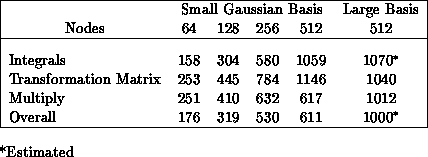
Table 8.6:
SMC Performance on the Delta (MFLOPS)
In the present state of the program, the perfectly parallel
integral-calculation step is the dominant element in most of our
calculations, as desired and expected based on the amount of
floating-point work. It is also the most complex step, however, with
little linear algebra but with many math library calls (sin, cos, exp,
sqrt), floating-point divides, and branches. Not surprisingly,
therefore, it is comparatively slow. We have timed the CRAY version at
 on a single-processor Y-MP, reflecting the routine's
intrinsically scalar character. Present performance on the i860 is
about
on a single-processor Y-MP, reflecting the routine's
intrinsically scalar character. Present performance on the i860 is
about  . Some additional optimization is planned,
but substantial improvement may have to await more mature versions of
the compiler and libraries.
. Some additional optimization is planned,
but substantial improvement may have to await more mature versions of
the compiler and libraries.
Figure 8.10:
Calculated Integral Elastic Cross Sections for Electron Scattering
by the C H
H Isomers Cyclopropane and Propylene. For comparison,
experimental total cross sections of Refs. [Floeder:85a] (open symbols) and
[Nishimura:91a] (filled symbols) are shown; triangles are cyclopropane and
circles propylene data.
Isomers Cyclopropane and Propylene. For comparison,
experimental total cross sections of Refs. [Floeder:85a] (open symbols) and
[Nishimura:91a] (filled symbols) are shown; triangles are cyclopropane and
circles propylene data.
With the program components as described above, the present code should
run on 512 nodes of the Delta at a sustained rate of approximately  . In practice, lower performance is obtained, due to
synchronization delays, load imbalance, file I/O,
etc.
Actual timings taken from 64- to 512-node production runs are given in
Table
8.6
. The limited data available for the
integral-evaluation package reflects the difficulty of obtaining an
accurate operation count; for the case shown, a count was obtained
using flow-tracing utilities on a CRAY. For the ``large'' case shown
in the table, we estimate overall performance at
. In practice, lower performance is obtained, due to
synchronization delays, load imbalance, file I/O,
etc.
Actual timings taken from 64- to 512-node production runs are given in
Table
8.6
. The limited data available for the
integral-evaluation package reflects the difficulty of obtaining an
accurate operation count; for the case shown, a count was obtained
using flow-tracing utilities on a CRAY. For the ``large'' case shown
in the table, we estimate overall performance at  ,
inclusive of all I/O and overhead, on 512 nodes of the Delta; this
estimate is based on an approximate operation count for the integral
package and actual counts for the remaining routines.
,
inclusive of all I/O and overhead, on 512 nodes of the Delta; this
estimate is based on an approximate operation count for the integral
package and actual counts for the remaining routines.
Next:
8.3.5 Selected Results
Up:
8.3.4 Performance
Previous:
Mark IIIfp
Guy Robinson
Wed Mar 1 10:19:35 EST 1995
8.3.5 Selected Results
Next:
8.3.6 Conclusion
Up:
Studies of Electron-Molecule
Previous:
Intel Machines
The distributed-memory SMC program has been applied to a number of elastic
and inelastic electron-molecule scattering problems, emphasizing polyatomic
gases of interest in low-temperature plasma applications [
JTIS:88a
],
[
Manos:89a
]. Initial applications [
Hipes:90a
],
[
Winstead:91d
]
on the Mark IIIfp were to elastic scattering by ethylene (C H
H ), ethane
(C
), ethane
(C H
H ), propane (C
 H
H ), disilane (Si
 H
H ), germane
(GeH
), germane
(GeH ), and tetrafluorosilane (SiF
 ). We have since studied elastic
scattering by other systems, including phosphine (PH
). We have since studied elastic
scattering by other systems, including phosphine (PH ), propylene
(C
), propylene
(C H
H ) and its isomer cyclopropane,
n
-butane (C
) and its isomer cyclopropane,
n
-butane (C H
H ), and
1,2-
trans
-difluoroethylene, both on the Mark IIIfp and on the Intel
machines. We have also examined inelastic collisions with ethylene
[
Sun:92a
], formaldehyde (CH
), and
1,2-
trans
-difluoroethylene, both on the Mark IIIfp and on the Intel
machines. We have also examined inelastic collisions with ethylene
[
Sun:92a
], formaldehyde (CH O), methane (CH
 ), and silane
(SiH
), and silane
(SiH ). Below we present selected results of these calculations, where
possible comparing to experimental data.
). Below we present selected results of these calculations, where
possible comparing to experimental data.
Figure
8.10
shows integral elastic cross sections-that is,
cross sections summed over all angles of scattering, plotted as a function of
the electron's kinetic energy-for the two C H
H isomers, cyclopropane
and propylene. Scattering from propylene requires some special
consideration, because of its small dipole moment [
Winstead:92a
]. These
calculations were performed in the static-exchange approximation, neglecting
polarization and excitation effects, on 256-node partitions of the Delta.
The results in Figure
8.10
should be considered preliminary,
since studies to test convergence
of the cross
section with respect to basis set are in progress, but we do not expect
major changes at the energies shown. Corresponding experimental values
have not been reported, but the total scattering cross section, of
which elastic scattering is the dominant component, has been measured
[
Floeder:85a
], [
Nishimura:91a
], and these data are included
in Figure
8.10
. Both the calculation and the measurements
show a clear isomer effect in the vicinity of the broad maximum, which
gradually lessens at higher energies. At the level of approximation
(static-exchange) used in these calculations, the maxima in the cross
sections are expected to appear shifted to higher energies and
somewhat broadened and lowered in intensity. Thus, for propylene, where
some discrepancy is seen between the two measurements, our calculation
appears to support the larger values of [
Nishimura:91a
].
isomers, cyclopropane
and propylene. Scattering from propylene requires some special
consideration, because of its small dipole moment [
Winstead:92a
]. These
calculations were performed in the static-exchange approximation, neglecting
polarization and excitation effects, on 256-node partitions of the Delta.
The results in Figure
8.10
should be considered preliminary,
since studies to test convergence
of the cross
section with respect to basis set are in progress, but we do not expect
major changes at the energies shown. Corresponding experimental values
have not been reported, but the total scattering cross section, of
which elastic scattering is the dominant component, has been measured
[
Floeder:85a
], [
Nishimura:91a
], and these data are included
in Figure
8.10
. Both the calculation and the measurements
show a clear isomer effect in the vicinity of the broad maximum, which
gradually lessens at higher energies. At the level of approximation
(static-exchange) used in these calculations, the maxima in the cross
sections are expected to appear shifted to higher energies and
somewhat broadened and lowered in intensity. Thus, for propylene, where
some discrepancy is seen between the two measurements, our calculation
appears to support the larger values of [
Nishimura:91a
].
Figure 8.11:
Differential Cross Sections for Elastic Scattering of  Electrons by Disilane and Ethane. Experimental points for ethane (circles)
are from Ref. [Tanaka:88a]; disilane data (squares) are from Ref.
[Tanaka:89a].
Electrons by Disilane and Ethane. Experimental points for ethane (circles)
are from Ref. [Tanaka:88a]; disilane data (squares) are from Ref.
[Tanaka:89a].
Figure
8.11
shows the plotting of the calculated
differential cross section, that is, the cross section as a function of
scattering angle, for elastic scattering of  electrons from
ethane and its analogue disilane. These results were obtained on the
Mark IIIfp within the static-approximation. Agreement with experiment
[Tanaka:88a;89a], is quite
good; although there are quantitative differences where the magnitude
of the cross section is small, the qualitative features are well
reproduced for both molecules.
electrons from
ethane and its analogue disilane. These results were obtained on the
Mark IIIfp within the static-approximation. Agreement with experiment
[Tanaka:88a;89a], is quite
good; although there are quantitative differences where the magnitude
of the cross section is small, the qualitative features are well
reproduced for both molecules.
Calculations of electronic excitation cross sections are shown in
Figures
8.12
and
8.13
. In
Figure
8.12
, we present the integral cross section for
excitation of the  state of ethylene
[
Sun:92a
], obtained on the Mark IIIfp in a two-channel approximation.
This
state of ethylene
[
Sun:92a
], obtained on the Mark IIIfp in a two-channel approximation.
This  excitation weakens the C-C bond, and its cross
section is relevant to the dissociation of ethylene by low-energy electron
impact. As seen in the figure, the cross section increases rapidly from
threshold (experimental value
excitation weakens the C-C bond, and its cross
section is relevant to the dissociation of ethylene by low-energy electron
impact. As seen in the figure, the cross section increases rapidly from
threshold (experimental value  ) and reaches a fairly high peak
value before beginning a gradual decline. The threshold rise is largely due
to a
d
-wave (
) and reaches a fairly high peak
value before beginning a gradual decline. The threshold rise is largely due
to a
d
-wave ( ) contribution, seen as a shoulder around
 above threshold, which may arise from a core-excited shape
resonance. Relative measurements of this cross section [
Veen:76a
],
which we have placed on an absolute scale by normalizing to our calculated
value at the broad maximum, show a much sharper structure near threshold, but
are otherwise in good agreement.
above threshold, which may arise from a core-excited shape
resonance. Relative measurements of this cross section [
Veen:76a
],
which we have placed on an absolute scale by normalizing to our calculated
value at the broad maximum, show a much sharper structure near threshold, but
are otherwise in good agreement.
Figure 8.12:
Integral Cross Section for Electron-Impact Excitation of the
 State of Ethylene. Solid line: present
two-channel result; dashed line: relative measurement of Ref. [Veen:76a],
normalized to the calculated value at the broad maximum.
State of Ethylene. Solid line: present
two-channel result; dashed line: relative measurement of Ref. [Veen:76a],
normalized to the calculated value at the broad maximum.
Figure
8.13
shows the cross section for electron-impact
excitation of the  and
and  states of formaldehyde, obtained from a three-channel calculation. Portions
of this calculation were done on the Mark IIIfp, the iPSC/860, and the Delta.
Experimental data for these excitations are not available, but an independent
calculation at a similar level of theory has been reported
[
Rescigno:90a
], and is shown in the figure. Since the complex-Kohn
calculation of [
Rescigno:90a
] included only partial waves up to
states of formaldehyde, obtained from a three-channel calculation. Portions
of this calculation were done on the Mark IIIfp, the iPSC/860, and the Delta.
Experimental data for these excitations are not available, but an independent
calculation at a similar level of theory has been reported
[
Rescigno:90a
], and is shown in the figure. Since the complex-Kohn
calculation of [
Rescigno:90a
] included only partial waves up to
 , we show both the full SMC result, obtained from
  , and a restricted SMC result, obtained with
f
projected onto a
spherical-harmonic basis
, and a restricted SMC result, obtained with
f
projected onto a
spherical-harmonic basis  ,
,  . The agreement
between the restricted SMC result and that of [
Rescigno:90a
] is in
general excellent; however, comparison to the full SMC result indicates
that such a restriction introduces some errors at higher energies.
. The agreement
between the restricted SMC result and that of [
Rescigno:90a
] is in
general excellent; however, comparison to the full SMC result indicates
that such a restriction introduces some errors at higher energies.
Figure 8.13:
Calculated Integral Cross Sections for Electron-Impact Excitation of
the  and
and  States of
Formaldehyde, Obtained from Three-Channel Calculations. Solid lines:
present SMC results; short-dashed lines: SMC results, limited to
States of
Formaldehyde, Obtained from Three-Channel Calculations. Solid lines:
present SMC results; short-dashed lines: SMC results, limited to
 ; long-dashed lines: complex-Kohn calculations of Ref.\
[Rescigno:90a].
; long-dashed lines: complex-Kohn calculations of Ref.\
[Rescigno:90a].
Next:
8.3.6 Conclusion
Up:
Studies of Electron-Molecule
Previous:
Intel Machines
Guy Robinson
Wed Mar 1 10:19:35 EST 1995
8.3.6 Conclusion
Next:
9 Loosely Synchronous Problems
Up:
Studies of Electron-Molecule
Previous:
8.3.5 Selected Results
The concurrent implementation of a large sequential code which is in
production on CRAY-type
machines is a type of project
which is likely to become increasingly common as commercial parallel
machines proliferate and ``mainstream'' computer users are attracted by
their potential. Several lessons which emerge from the port of the SMC
code may prove useful to those contemplating similar projects. One is
the value of focusing on the concurrent implementation and, so far as
possible, avoiding or deferring minor improvements. If the original
code is a reasonably effective production tool, such tinkering is
unlikely to be of great enough benefit to justify the distraction from
the primary goal of achieving a working concurrent version. On the
other hand, major issues of structure and organization which bear
directly on the parallel conversion deserve very careful attention, and
should ideally be thought through before the actual conversion has
begun. In the SMC case, the principal such issue was how to implement
efficiently the transformation from primitive integrals to physical
matrix elements. The solution arrived at not only suggested that a
significant departure from the sequential code was warranted but also
determined the data decomposition. A further point worth mentioning is
that the conversion was greatly facilitated by the C P environment
which fostered collaboration between workers familiar with the original
code and its application, and workers adept at parallel programming
practice, and in which there was ready access both to smaller machines
for debugging
runs and to larger production machines.
Finally, we believe that the emphasis on achieving a simple
communication strategy has justified itself in practice, not only in
efficiency but in the portability and reliability of the program.
P environment
which fostered collaboration between workers familiar with the original
code and its application, and workers adept at parallel programming
practice, and in which there was ready access both to smaller machines
for debugging
runs and to larger production machines.
Finally, we believe that the emphasis on achieving a simple
communication strategy has justified itself in practice, not only in
efficiency but in the portability and reliability of the program.
At present the parallel SMC code is essentially in production mode, all
capabilities of the original sequential code having been implemented and some
optimization performed. Further optimization of the primitive-integral
package is in progress, but the major focus in the near future is likely to
be applications on the one hand and extending the capabilities of the
parallel code on the other. We are particularly interested in modifying
the program to allow the study of electron scattering from open-shell systems
(i.e., those with unpaired electrons), with a view to obtaining cross
sections for some of the more important polyatomic species found in
materials-processing plasmas. With continued progress in parallel hardware,
we are very optimistic about the prospects for theory to make a substantial
contribution to our knowledge of electron-polyatomic collisions.
Next:
9 Loosely Synchronous Problems
Up:
Studies of Electron-Molecule
Previous:
8.3.5 Selected Results
Guy Robinson
Wed Mar 1 10:19:35 EST 1995
9 Loosely Synchronous Problems
Next:
9.1 Problem Structure
Up:
Parallel Computing Works
Previous:
8.3.6 Conclusion
Guy Robinson
Wed Mar 1 10:19:35 EST 1995
9.1 Problem Structure
Next:
Geomorphology by Micromechanical
Up:
9 Loosely Synchronous Problems
Previous:
9 Loosely Synchronous Problems
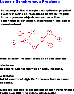
Figure 9.1:
The Loosely Synchronous Problem Class
The significance of loosely synchronous
problems and their natural parallelism was an important realization
that emerged gradually (perhaps in 1987 as a clear concept) as we
accumulated results from C P research. As described in
Figure
9.1
, fundamental theories often describe phenomena
in terms of a set of similar entities obeying a single law. However,
one does not usually describe practical problems in terms of their
fundamental description in a theory such as QCD in Section
4.3
.
Rather, we use macroscopic concepts. Looking at society, a particle
physicist might view it as a bunch of quarks and gluons; a nuclear
physicist as a collection of protons and neutrons; a chemist as a
collection of molecules; a biochemist as a set of proteins; a
biologist as myriad cells; and a social scientist as a collection of
people. Each description is appropriate to answer certain questions,
and it is usually clear which description should be used. If we
consider a simulation of society, or a part there of, only the QCD
description is naturally synchronous. The other fields view society as
a set of macroscopic constructs, which are no longer identical and
typically have an irregular interconnect. This is caricatured in
Figure
9.1
as an irregular network. The simulation is
still data-parallel and, further, there is a critical macroscopic
synchronization-in a time-stepped simulation at every time step
P research. As described in
Figure
9.1
, fundamental theories often describe phenomena
in terms of a set of similar entities obeying a single law. However,
one does not usually describe practical problems in terms of their
fundamental description in a theory such as QCD in Section
4.3
.
Rather, we use macroscopic concepts. Looking at society, a particle
physicist might view it as a bunch of quarks and gluons; a nuclear
physicist as a collection of protons and neutrons; a chemist as a
collection of molecules; a biochemist as a set of proteins; a
biologist as myriad cells; and a social scientist as a collection of
people. Each description is appropriate to answer certain questions,
and it is usually clear which description should be used. If we
consider a simulation of society, or a part there of, only the QCD
description is naturally synchronous. The other fields view society as
a set of macroscopic constructs, which are no longer identical and
typically have an irregular interconnect. This is caricatured in
Figure
9.1
as an irregular network. The simulation is
still data-parallel and, further, there is a critical macroscopic
synchronization-in a time-stepped simulation at every time step
 ,
,  ,
,  . This is an algorithmic
synchronization that ensures natural scaling parallelism, that is, that
the efficiency of Equations
3.10
and
3.11
is
given by
. This is an algorithmic
synchronization that ensures natural scaling parallelism, that is, that
the efficiency of Equations
3.10
and
3.11
is
given by

and

with the parameter  of Equation
3.10
equal
to zero.
of Equation
3.10
equal
to zero.  is given by Equation
3.10
in terms
of the system dimension.
The efficiency only
depends on the problem grain size and not explicitly on the number of
processing nodes. As emphasized in [
Gustafson:88a
], these
problems scale so that if one doubles both the machine and problem
size, the speedup will also double with constant efficiency. This
situation is summarized in Figure
9.2
.
is given by Equation
3.10
in terms
of the system dimension.
The efficiency only
depends on the problem grain size and not explicitly on the number of
processing nodes. As emphasized in [
Gustafson:88a
], these
problems scale so that if one doubles both the machine and problem
size, the speedup will also double with constant efficiency. This
situation is summarized in Figure
9.2
.
Figure 9.2:
Speedup as a Function of Number of Processors 
Why is there no synchronization overhead in this problem class?
Picturesquely, we can say that the processors ``know'' that they are
synchronized at the end of each algorithmic time step. We use time in
the generalized complex system
language of
Section
3.3
and so it would represent, for instance,
iteration number in a matrix problem. Operationally, we can describe
the loosely synchronous class on a MIMD machine by the
communication-calculation sequence in Figure
9.3
. The
update (calculate) phase can involve very different algorithms and
computations for the points stored in different processors. Thus, a
MIMD architecture is needed in the general case. Synchronization is
provided, as in Figure
9.3
by the internode communication
phases at each time step. As described in Chapters
5
and
16
, this does not need, but certainly can use, the full
asynchronous message-passing capability of a MIMD machine.
Figure 9.3:
Communication-Calculation Phases in a Loosely Synchronous
Problem
We have split the loosely synchronous problems into two chapters,
with those in Chapter
12
showing more irregularities and
greater need for MIMD architectures than the applications described in
this chapter. There has been no definitive
study of which loosely synchronous problems can run well on SIMD
machines. Some certainly can, but not all. We have discussed some
of these issues in Section
6.1
. If, as many expect, SIMD
will remain a cost-effective architecture offered commercially, it
will be important to better clarify the class of irregular problems
that definitely need the full MIMD architecture.
As mentioned above, the applications in this chapter are ``modestly''
loosely synchronous. They include particle simulations
(Sections
9.2
and
9.3
), solutions of partial
differential equation (Sections
9.3
,
9.4
,
9.5
,
9.7
), and circuit simulation (Sections
9.5
and
9.6
). In Section
9.8
, we describe an optimal
assignment algorithm that can be used for multiple target Kalman
filters
and was developed for the large scale
battle management simulation of Sections
18.3
and
18.4
. Section
9.9
covers the parallelization of
learning (``back-propagation'') neural nets with improved learning
methods. An interesting C P application not covered in detail in
this book was the calculation of an exchange energy in solid
P application not covered in detail in
this book was the calculation of an exchange energy in solid  at temperatures below
  [Callahan:88a;88b].
This was our first major
use of the nCUBE-1 in production mode and Callahan suffered all the
difficulties of a pioneer with the, at the time, decidely unreliable
hardware and software. He used 250 hours on our 512-node
nCUBE-1,
which was equivalent to 1000 hours of a
non-vectorized
CRAY X-MP
implementation. In discussing
SIMD versus MIMD, one usually concentrates on the synchronization
aspects. However, Callahan's application illustrates another point;
namely, commercial SIMD machines typically have many more processors
than a comparable MIMD computer. For example, Thinking Machines
introduced the 32-node MIMD CM-5 as roughly equivalent (in price) to an
[Callahan:88a;88b].
This was our first major
use of the nCUBE-1 in production mode and Callahan suffered all the
difficulties of a pioneer with the, at the time, decidely unreliable
hardware and software. He used 250 hours on our 512-node
nCUBE-1,
which was equivalent to 1000 hours of a
non-vectorized
CRAY X-MP
implementation. In discussing
SIMD versus MIMD, one usually concentrates on the synchronization
aspects. However, Callahan's application illustrates another point;
namely, commercial SIMD machines typically have many more processors
than a comparable MIMD computer. For example, Thinking Machines
introduced the 32-node MIMD CM-5 as roughly equivalent (in price) to an
 SIMD CM-2. The SIMD architecture has 256 times as many
nodes. Of course, the SIMD nodes are much simpler, but this still
implies that one needs a large enough problem to exploit this extra
number of nodes. There are some coarse-grain SIMD
machines-especially special-purpose QCD machines [
Battista:92a
],
[
Christ:86a
], [
Fox:93a
], [
Marinari:93a
]-but it is more
natural to build fine-grain machines. If the node is large, one might
as well add MIMD capability! Full matrix
algorithms, such as LU decomposition,
(see Chapter
8
), are often
synchronous, but do not perform very well on SIMD machines due to
insufficient parallelism [
Fox:92j
]. Many of the operations only
involve single rows and columns and have severe load imbalance on
fine-grain machines. Callahan's
SIMD CM-2. The SIMD architecture has 256 times as many
nodes. Of course, the SIMD nodes are much simpler, but this still
implies that one needs a large enough problem to exploit this extra
number of nodes. There are some coarse-grain SIMD
machines-especially special-purpose QCD machines [
Battista:92a
],
[
Christ:86a
], [
Fox:93a
], [
Marinari:93a
]-but it is more
natural to build fine-grain machines. If the node is large, one might
as well add MIMD capability! Full matrix
algorithms, such as LU decomposition,
(see Chapter
8
), are often
synchronous, but do not perform very well on SIMD machines due to
insufficient parallelism [
Fox:92j
]. Many of the operations only
involve single rows and columns and have severe load imbalance on
fine-grain machines. Callahan's  application did not exhibit
``massive'' parallelism, and so ``had'' to use a MIMD machine
irrespective of his problem's temporal structure.
He used 512 nodes on the nCUBE-1 by combining three forms of
parallelism: Two came from the problem formulation with spatial and
temporal parallelism, the other from running four different parameter
values concurrently.
application did not exhibit
``massive'' parallelism, and so ``had'' to use a MIMD machine
irrespective of his problem's temporal structure.
He used 512 nodes on the nCUBE-1 by combining three forms of
parallelism: Two came from the problem formulation with spatial and
temporal parallelism, the other from running four different parameter
values concurrently.
A polymer
simulation [Ding:88a;88b] [
Ding:88a
]
[
Ding:88b
] by Ding and Goddard, using the reptation method,
exhibited a similar effect. There is a chain of
N
chemical units and
the algorithm involves special treatment of the two units at the
beginning and end of the linear polymer. The MIMD program ran
successfully on the Mark III and FPS
T-Series, but the
problem is too ``small'' (parallelism of  ) for this algorithm to
run on a SIMD machine even though most of the basic operations can be
run synchronously.
) for this algorithm to
run on a SIMD machine even though most of the basic operations can be
run synchronously.
This issue of available parallelism also complicates the implementation of
multigrid algorithms on SIMD machines [Frederickson:88a;88b;89a;89b].
Next:
Geomorphology by Micromechanical
Up:
9 Loosely Synchronous Problems
Previous:
9 Loosely Synchronous Problems
Guy Robinson
Wed Mar 1 10:19:35 EST 1995
Geomorphology by Micromechanical
Simulations
Next:
Plasma Particle-in-Cell
Simulation
Up:
9 Loosely Synchronous Problems
Previous:
9.1 Problem Structure
Geomorphology
is the study of the small-scale
surface evolution of the earth under the forces resulting from such agents as
wind, water, gravity, and ice. Understanding and prediction in
geomorphology are critically dependent upon the ability to model the
processes that shape the landscape. Because these processes in general
are too complicated on large scales to describe in detail, it is
necessary to adopt a system of hierarchical models in which the
behavior of small systems is summarized by a set of rules governing the
next larger system; in essence, these rules constitute a simplified
algorithm for the physical processes in the smaller system that cannot
be treated fully at larger scales. A significant fraction of the
processes in geomorphology involve entrainment, transport and
deposition of particulate matter. Where the intergrain forces become
comparable to or greater than the forces arising from the transporting
agents, consideration of the properties of a granular material, a
system of grains which collide with the slide against neighboring
grains, is warranted. A micromechanical description of granular
materials has proved difficult, except in energetic flow regimes
[
Haff:83a
], [
Jenkins:83a
]. Thus, researchers have turned to
dynamical and computer simulations at the level of individual grains in
order to elucidate some of the basic mechanical properties of granular
materials
([
Cundall:79a
],
[
Walton:83a
] pioneered this simulation technique). In this
section, we discuss the role that hypercube concurrent processing has
played and is expected to play both in grain-level dynamical
simulations and in relating these simulations to modelling the
formation and evolution of landforms.
As an example of this approach to geomorphology, we shall consider
efforts to model transport of sand
by the wind based upon the
grain-to-grain dynamics. Sand is transported by the wind primarily in
saltation
and in reptation [
Bagnold:41a
]. Saltating
grains are
propelled along the surface in short hops by the wind. Each collision
between a saltating sand grain and the surface results in a loss of
energy which is compensated, on the average, by energy acquired from the
wind. Reptating grains are ejected from the sand surface by saltating
grain-sand bed impacts; they generally come to rest shortly after
returning to the sand surface.
Computer simulations of saltating grain impacts upon a loose grain bed
were performed on an early version of the hypercube [Werner:88a;88b].
Collisions between a single
impacting grain and a box of 384 circular grains were simulated. The
grains interact through stiff, inelastic compressional contact forces
plus a Coulomb friction force. The equations of motion for the
particles are integrated forward in time using a predictor-corrector
technique. At each step in time, the program checks for contacts
between particles and, where contacts exist, computes the contact
forces. Dynamical simulations of granular materials are
computationally intensive, because the time scale of the interaction
between grains (tens of microseconds) is much smaller than the time
scale of the simulation (order one second).
The simulation was decomposed on a Caltech hypercube by assigning the
processors to regions of space lying on a rectangular grid. The
computation time is a combination of calculation time in each processor
due to contact searches and to force computations, and of communication
time in sending information concerning grain positions and velocities
to neighboring processors for interparticle force calculations on
processor boundaries. Because the force computation is complicated,
the communication time was found to be a negligible fraction of the
total computation time for granular materials in which enduring
intergrain contacts are dominant. The boundaries between processors
are changed incrementally throughout the calculation in order to
balance the computational load among the processors. The optimal
decomposition has enough particles per processor to diminish the
relative importance of statistical fluctuations in the load, and a
system of boundaries which conforms as much as possible to the geometry
of the problem. For grain-bed impacts, efficiencies between 0.89 and
0.97 were achieved [
Werner:88a
].
Irregularities of the geometry are important in determining which
sand grains interact with each other. Thus, it is not possible to
find an efficient synchronous algorithm for this and many other particle
interaction problems. The very irregular inhomogeneous
astrophysical calculations described in Section
12.4
illustrate this point clearly. One also finds the same issue in
molecular dynamics
codes, such as CHARMM
which are extensively used in chemistry.
This problem
is, however, loosely synchronous as we can naturally macroscopically
synchronize the calculation after each time step-thus a MIMD
implementation where each processor processes its own irregular
collection of grains is very natural and efficient. The sand grain
problem, unlike that of Section
12.4
, has purely local forces as
the grains must be in physical contact to affect each other. Thus,
only very localized communication is necessary. Note that
Section
4.5
describes a synchronous formulation of this
problem.
The results of the grain-bed impact simulations have facilitated
treatment of two larger scale problems. A simulation of steady-state
saltation in which calculation of saltating grain trajectories and
modifications to the wind velocity profile, due to acceleration of
saltating grains, were combined with a grain-bed impact distribution
function derived from experiments and simulations. This simulation yielded
such characteristics of saltation as flux and erosive potential
[
Werner:90a
]. A simulation of the rearrangement of surface grains
in reptation led to the formation of self-organized small-scale bedforms,
which resemble wind ripples in both size and shape [
Landry:93a
],
[Werner:91a;93a]. Larger, more complicated ripple
formation simulations and a simulation of sand dune formation, using a
similar approach which is under development, are problems that will
require a combination of processing power and memory not available on
present supercomputers. Ripple and dune simulations are expected to
run efficiently with a spatial decomposition on a hypercube.
Water is an important agent for the transport of sediment. Unlike
wind-blown sand transport, underwater sand transport requires
simultaneous simulation of the grains and the fluid because water and
sand are similar in density. We are developing a grain/fluid mixture
simulation code for a hypercube in which the fluid is modelled by a gas
composed of elastic hard circles (spheres in three dimensions). The
simulation steps the gas forward at discrete time intervals, allowing
the gas particles to collide (with another gas particle or a
macroscopic grain) only once per step. The fluid velocity and the fluid
force on each grain are computed by averaging. Since a typical void
between macroscopic grains will be occupied by up to 1000 gas particles,
the requisite computational speed and memory capacity can be found only
in the hypercube architecture. Communication is expected to be minimal
and load balancing can be accomplished for a sufficiently large system.
It is expected that larger scale simulations of erosion and deposition
by water [
Ahnert:87a
] will benefit from the findings of the
fluid/grain mixture simulations. Also, these large-scale landscape
evolution simulations are suitable themselves for a MIMD parallel
machine.
Computer simulation is assuming an increasing role in geomorphology.
We suggest that the development and availability of high-performance
MIMD concurrent processors will have considerable influence upon the
future of computing in geomorphology.
Next:
Plasma Particle-in-Cell
Simulation
Up:
9 Loosely Synchronous Problems
Previous:
9.1 Problem Structure
Guy Robinson
Wed Mar 1 10:19:35 EST 1995
Plasma Particle-in-Cell
Simulation of anElectron Beam Plasma Instability
Next:
9.3.1 Introduction
Up:
9 Loosely Synchronous Problems
Previous:
Geomorphology by Micromechanical
Guy Robinson
Wed Mar 1 10:19:35 EST 1995
9.3.1 Introduction
Next:
9.3.2 GCPIC Algorithm
Up:
Plasma Particle-in-Cell
Simulation
Previous:
Plasma Particle-in-Cell
Simulation
Plasmas-gases
of electrically charged particles-are
one of the most complex fluids encountered in nature. Because of the
long-range nature of the electric and magnetic interactions between
plasma electrons and the ions composing them, plasmas exhibit a wide
variety of collective forms of motions, for example, coherent motions of large
number of electrons, ions, or both. This leads to an extremely rich
physics of plasmas. Plasma particle-in-cell
(PIC) simulation codes have proven to be a powerful tool for
the study of complex nonlinear plasma problems in many areas of plasma
physics research such as space and astrophysical plasmas, magnetic and
inertial confinement, free electron lasers, electron and ion beam
propagation and particle accelerators. In PIC codes, the orbits of
thousands to millions of interacting plasma electrons and ions are
followed in time as the particles move in electromagnetic fields
calculated self-consistently from the charge and current densities
created by these same plasma particles.
We developed an algorithm, called the
general concurrent
particle-in-cell algorithm
(GCPIC) for implementing PIC codes
efficiently on MIMD parallel computers [
Liewer:89c
]. This
algorithm was first used to implement a well-benchmarked [
Decyk:88a
]
one-dimensional electrostatic PIC code. The benchmark problem, used to
benchmark the Mark IIIfp, was a simulation of an electron beam plasma
instability ([
Decyk:88a
], [
Liewer:89c
]). Dynamic load
balancing
has been implemented in a
one-dimensional electromagnetic
GCPIC code
[
Liewer:90a
]; this code was used to study electron
dynamics
in magnetosonic shock waves in space
plasmas [
Liewer:91a
]. A two-dimensional electrostatic PIC code
has also been implemented using the GCPIC algorithm with and without
dynamic load balancing [Ferraro:90b;93a].
More recently, the two-dimensional electrostatic
GCPIC code was extended to an electromagnetic code [
Krucken:91a
]
and used to study parametric instabilities of large amplitude Alfvén
waves in space plasmas [
Liewer:92a
].
Guy Robinson
Wed Mar 1 10:19:35 EST 1995
9.3.2 GCPIC Algorithm
Next:
9.3.3 Electron Beam Plasma
Up:
Plasma Particle-in-Cell
Simulation
Previous:
9.3.1 Introduction
In plasma PIC codes, the orbits of the many interacting plasma electrons
and ions are followed as an initial value problem as the particles move in
self-consistently calculated electromagnetic fields. The fields are found by
solving Maxwell's equations,
or a subset,
with the plasma currents and charge density as source terms; the
electromagnetic fields determine the forces on the particles. In a PIC
code, the particles can be anywhere in the simulation
domain,
but the field equations are solved
on a discrete grid. At each time step in a PIC code, there are two
stages to the computation. In the first stage, the position and
velocities of the particles are updated by calculating the forces on
the particles from interpolation of the field values at the grid
points; the new charge and current densities at the grid points are
then calculated by interpolation from the new positions and velocities
of the particles. In the second stage, the updated fields are found by
solving the field equations on the grid using the new charge and
current densities. Generally, the first stage accounts for most of the
computation time because there are many more particles than grid
points.
The GCPIC algorithm [
Liewer:89c
] is designed to make the most
computationally intensive portion of a PIC code, which updates the
particles and the resulting charge and current densities, run
efficiently on a parallel processor. The time used to make these
updates is generally on the order of 90% of the total time for a
sequential code, with the remaining time divided between the
electromagnetic field solution and the diagnostic computations.
To implement a PIC code in parallel using the GCPIC algorithm, the physical
domain of the particle simulation is partitioned into subdomains, equal in
number to the number of processors, such that all subdomains have roughly
equal numbers of particles. For problems with nonuniform particle
densities, these subdomains will be of unequal physical size. Each
processor is assigned a subdomain and is responsible for storing the
particles and the electromagnetic field quantities for its subdomain and for
performing the particle computations for its particles. For a
one-dimensional code on a hypercube, nearest-neighbor subdomains are
assigned to nearest-neighbor processors. When particles move to new
subdomains, they are passed to the appropriate processor. As long as the
number of particles per subdomain is approximately equal, the processors'
computational loads will be balanced. Dynamic load balancing
is accomplished by repartitioning the simulations domain into
subdomains with roughly equal particle numbers when the processor loads
become sufficiently unbalanced. The computation of the new partitions,
done in a simple way using a crude approximation to the plasma density
profile, adds very little overhead to the parallel code.
The decomposition used for dividing the particles is termed the
primary decomposition
. Because the primary decomposition is not
generally the optimum one for the field solution on the grid, a
secondary decomposition
is used to divide the field computation.
The secondary decomposition remains fixed. At each time step, grid
data must be transferred between the two decompositions
[Ferraro:90b;93a],
[
Liewer:89c
].
The GCPIC algorithm has led to a very efficient parallel implementation of
the benchmarked one-dimensional electrostatic PIC code [
Liewer:89c
]. In
this electrostatic code, only forces from self-consistent (and external)
electric fields are included; neither an external nor a plasma-generated
magnetic field is included.
Next:
9.3.3 Electron Beam Plasma
Up:
Plasma Particle-in-Cell
Simulation
Previous:
9.3.1 Introduction
Guy Robinson
Wed Mar 1 10:19:35 EST 1995
9.3.3 Electron Beam Plasma Instability
Next:
Performance Results for
Up:
Plasma Particle-in-Cell
Simulation
Previous:
9.3.2 GCPIC Algorithm
The problem used to benchmark the one-dimensional electrostatic GCPIC code on
the Mark IIIfp was a simulation of an instability in a plasma due to the
presence of an electron beam. The six color pictures in Figure 9.4
(Color Plate) show results from this simulation from the
Mark IIIfp. Plotted is electron phase space-position versus velocity of
the electrons-at six times during the simulation. The horizontal axis is
the velocity and the vertical axis is the position of the electrons.
Initially, the background plasma electrons (magenta dots) have a Gaussian
distribution of velocities about zero. The width of the distribution in
velocity is a measure of the temperature of the electrons. The beam
electrons (yellow dots) stream through the background plasma at five times
the thermal velocity. The beam density was 10% of the density of the
background electrons. Initially, these have a Gaussian distribution about
the beam velocity. Both beam and background electrons are distributed
uniformly in
x
. This initial configuration is unstable to an electrostatic
plasma wave which grows by tapping the free energy of the electron beam. At
early times, the unstable waves grow exponentially. The influence of this
electrostatic wave on the electron phase space is shown in the subsequent
plots. The beam electrons lose energy to the wave. The wave acts to try to
``thermalize'' the electron's velocity distribution in the way collisions
would act in a classical fluid. At some point, the amplitude of the wave's
electrostatic potential is enough to ``trap'' some of the beam and background
electrons, leading the visible swirls in the phase space plots. This
trapping causes the wave to stop growing. In the end, the beam and
background electrons are mixed and the final distribution is ``hotter''
kinetic energy from the electron beam which has gone into heating both the
background and beam electrons.
Figure 9.4:
Time history of electron phase space in a
plasma PIC simulation of an electron beam plasma instability on the Mark
IIIfp hypercube. The horizontal axis is the electron velocity and the
vertical axis is the position. Initially, a small population of beam
electrons (green dots) stream through the background plasma electrons
(magenta dots). An electronic wave grows, tapping the energy in the
electron beam. The vortices in phase space at late times result from
electrons becoming trapped in the potential of the wave. See section 9.3 of
the text for further description.
Next:
Performance Results for
Up:
Plasma Particle-in-Cell
Simulation
Previous:
9.3.2 GCPIC Algorithm
Guy Robinson
Wed Mar 1 10:19:35 EST 1995
Performance Results for One-DimensionalElectrostatic Code
Next:
9.3.5 One-Dimensional Electromagnetic Code
Up:
Plasma Particle-in-Cell
Simulation
Previous:
9.3.3 Electron Beam Plasma
Timing results for the benchmark problem, using the one-dimensional code
without dynamic load balancing, are given in the tables. In
Table
9.1
, results for the
push time
are given for
various hypercube dimensions for the Mark III and Mark IIIfp hypercubes.
Here, we define the push time as the time per particle per time step to
update the particle positions and velocities (including the interpolation to
find the forces at the particle positions) and to
deposit
(interpolate) the particles' contributions to the charge and/or current
densities onto the grid. Table
9.1
shows the efficiency of the
push for runs in which the number of particles
increased linearly
with the number of processors used, so that the number of particles per
processor was constant (
fixed grain size
). The
efficiency
is
defined to be  , where
  is the run time
on
N
processors. In the ideal situation, a code's run time on
N
will be
is the run time
on
N
processors. In the ideal situation, a code's run time on
N
will be
 of its run time on one processor, and the efficiency is 100%. In
practice, communication between nodes and unequal processor loads leads to a
decrease in the efficiency.
of its run time on one processor, and the efficiency is 100%. In
practice, communication between nodes and unequal processor loads leads to a
decrease in the efficiency.
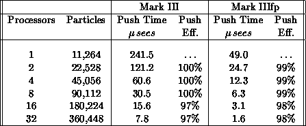
Table 9.1:
Hypercube Push Efficiency for Increasing Problem Size
The Mark III Hypercube consists of up to 64 independent processors, each with
four megabytes of dynamic random access memory and 128 kilobytes of static
RAM. Each processor consists of two Motorola MC68020 CPUs with a MC68882
Co-processor. The newer Mark IIIfp Hypercubes have, in addition, a Weitek
floating-point processor on each node. In Table
9.1
, push times
are given for both the Mark III processor (Motorola MC68882) and the
Mark IIIfp processor (Weitek). For the Weitek runs, the entire parallel code
was downloaded into the Weitek processors. The push time for the
one-dimensional electrostatic code has been benchmarked on many computers
[
Decyk:88a
]. Some of the times are given in Table
9.2
;
times for other computers can be found in [
Decyk:88a
]. For the Mark III
and Mark IIIfp runs, 720,896 particles were used (11,264 per processor);
for the other runs in Table
9.2
, 11,264 particles were used.
In all cases, the push time is the time per particle per time step to make
the particle updates. It can be seen that for the push portion of the code,
the 64-processor Mark IIIfp is nearly twice the speed of a one-processor
CRAY X-MP and 2.6 times the speed of a CRAY 2.
We have also compared the total run time for the benchmark code for a
case with 720,896 particles and 1024 grid points run for 1000 time
steps. The total run time on the 64-node Mark IIIfp was  ; on a one-processor CRAY 2,
  . For this
case, the 64-node Mark IIIfp was 1.6 times faster than the
CRAY 2
for the entire code. For the Mark IIIfp run,
about 10% of the total run time was spent in the initialization of the
particles, which is done sequentially.
. For this
case, the 64-node Mark IIIfp was 1.6 times faster than the
CRAY 2
for the entire code. For the Mark IIIfp run,
about 10% of the total run time was spent in the initialization of the
particles, which is done sequentially.
Benchmark times for the two-dimensional GCPIC code can be found in
[
Ferraro:90b
].
Next:
9.3.5 One-Dimensional Electromagnetic Code
Up:
Plasma Particle-in-Cell
Simulation
Previous:
9.3.3 Electron Beam Plasma
Guy Robinson
Wed Mar 1 10:19:35 EST 1995
9.3.5 One-Dimensional Electromagnetic Code
Next:
9.3.6 Dynamic Load Balancing
Up:
Plasma Particle-in-Cell
Simulation
Previous:
Performance Results for
The parallel one-dimensional electrostatic code was modified to include the
effects of external and self-consistent magnetic fields. This one-dimensional
electromagnetic code, with kinetic electrons and ions, has been used to
study electron dynamics in oblique collisionless shock waves such as in the
earth's bow shock. Forces on the particles are found from the fields at the
grid points by interpolation. For this code, with variation in the
x
direction only, the orbit equations for the
i
particle are

Motion is followed in the
x
direction only, but all three velocity
components must be calculated in order to calculate the  force. The longitudinal (along
x
) electric field is found by solving
Poisson's equation
force. The longitudinal (along
x
) electric field is found by solving
Poisson's equation

The transverse (to
x
) electromagnetic fields,  ,
,  ,
,  , and
, and
 , are found by solving

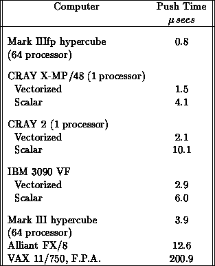
Table 9.2:
Comparison of Push Times on Various Computers
The plasma current density  and charge density
 are found at the grid points by interpolation from the
particle positions. Only the transverse (
y
and
z
) components of the
plasma current are needed. These coupled particle and field equations are
solved in time as an initial value problem. As in the electrostatic code,
the fields are solved by Fourier-transforming
the charge and
current densities and solving the equation in
k
space, and advancing
the Fourier components in time. External fields and currents can also
be included. At each time step, the fields are transformed back to
configuration space to calculate the forces needed to advance the
particles to the next time step. The hypercube FFT
routine
described in Section
12.4
was used in the one-dimensional
codes. Extending the existing parallel electrostatic code to include
the electromagnetic effects required no change in the parallel
decomposition of the code.
are found at the grid points by interpolation from the
particle positions. Only the transverse (
y
and
z
) components of the
plasma current are needed. These coupled particle and field equations are
solved in time as an initial value problem. As in the electrostatic code,
the fields are solved by Fourier-transforming
the charge and
current densities and solving the equation in
k
space, and advancing
the Fourier components in time. External fields and currents can also
be included. At each time step, the fields are transformed back to
configuration space to calculate the forces needed to advance the
particles to the next time step. The hypercube FFT
routine
described in Section
12.4
was used in the one-dimensional
codes. Extending the existing parallel electrostatic code to include
the electromagnetic effects required no change in the parallel
decomposition of the code.
Guy Robinson
Wed Mar 1 10:19:35 EST 1995
9.3.6 Dynamic Load Balancing
Next:
9.3.7 Summary
Up:
Plasma Particle-in-Cell
Simulation
Previous:
9.3.5 One-Dimensional Electromagnetic Code
In the GCPIC electrostatic code, the partitioning of the grid was static. The
grid was partitioned so that the computational load of the processors was
initially balanced. As simulations progress and particles move among
processors, the spatial distribution of the particles can change, leading to
load imbalance. This can severely degrade the parallel efficiency of the
push stage of the computation. To avoid this, dynamic load
balancing
has been implemented in a one-dimensional
electromagnetic code [
Liewer:90a
] and a two-dimensional electrostatic
code [
Ferraro:93a
].
To implement dynamic load balancing,
the grid is
repartitioned into new subdomains with roughly equal numbers of
particles as the simulation progresses. The repartitioning is not done
at every time step. The load imbalance is monitored at a
user-specified interval. When the imbalance becomes sufficiently
large, the grid is repartitioned and the particles moved to the
appropriate processors, as necessary. The load was judged sufficiently
imbalanced to warrant load balancing when the number of particles per
processor deviated from the ideal value  (= number of
particles/number of processors) by
(= number of
particles/number of processors) by  , for example,
twice the statistical fluctuation level.
, for example,
twice the statistical fluctuation level.
The dynamic load balancing is performed during the push stage of the
computation. Specifically, the new grid partitions are computed after
the particle positions have been updated, but before the particles are
moved to new processors to avoid an unnecessary moving of particles.
If the loads are sufficiently balanced, the subroutine computing the
new grid partitions is not called. The subroutine, which moves the
particles to appropriate processors, is called in either case.
To accurately represent the physics, a particle cannot move more than one
grid cell per time step. As a result, in the static one-dimensional code,
the routine which moves particles to new processors only had to move particles
to nearest-neighbor processors. To implement dynamic load balancing, this
subroutine had to be modified to allow particles to be moved to processors
any number of steps away. Moving the particles to new processors after grid
repartitioning can add significant overhead; however, this is incurred only
at time steps when load balancing occurs.
The new grid partitions are computed by a very simple method which adds
very little overhead to the parallel code. Each processor constructs
an approximation to the plasma density profile,  , and uses
this to compute the grid partitioning to load balance.
To construct the approximate density profile, each processor
sends the locations of its current subdomain boundaries and its current
number of particles to all other processors. From this information,
each processor can compute the average plasma density in each processor
and from this can create the approximate-to-density profile (with as
many points as processors). This approximate profile is used to
compute the grid partitioning which approximately divides the particles
equally among the processors. This is done by determining the set of
subdomain boundaries
, and uses
this to compute the grid partitioning to load balance.
To construct the approximate density profile, each processor
sends the locations of its current subdomain boundaries and its current
number of particles to all other processors. From this information,
each processor can compute the average plasma density in each processor
and from this can create the approximate-to-density profile (with as
many points as processors). This approximate profile is used to
compute the grid partitioning which approximately divides the particles
equally among the processors. This is done by determining the set of
subdomain boundaries  and
and  such that

Linear interpolation of the approximate profile is used in the numerical
integration. The actual plasma density profile could also be used in the
integration to determine the partitions. No additional computation would be
necessary to obtain the local (within a processor)  because it
is already computed for the field solution stage. However, it would
require more communication to make the density profile global. Other
methods of calculating new subdomain boundaries, such as sorting
particles, require a much larger amount of communication and
computational overhead.
because it
is already computed for the field solution stage. However, it would
require more communication to make the density profile global. Other
methods of calculating new subdomain boundaries, such as sorting
particles, require a much larger amount of communication and
computational overhead.
Next:
9.3.7 Summary
Up:
Plasma Particle-in-Cell
Simulation
Previous:
9.3.5 One-Dimensional Electromagnetic Code
Guy Robinson
Wed Mar 1 10:19:35 EST 1995
9.3.7 Summary
Next:
9.4 Computational Electromagnetics
Up:
Plasma Particle-in-Cell
Simulation
Previous:
9.3.6 Dynamic Load Balancing
The GCPIC algorithm was developed and implemented by Paulett C. Liewer, Jet
Propulsion Laboratory, Caltech, and Viktor K. Decyk, Physics Department,
University of California, Los Angeles. R. D. Ferraro, Jet Propulsion
Laboratory, Caltech, implemented the two-dimensional electrostatic PIC
code using the GCPIC algorithm with dynamic load balancing.
Guy Robinson
Wed Mar 1 10:19:35 EST 1995
9.4 Computational Electromagnetics
Next:
LU Factorization of
Up:
9 Loosely Synchronous Problems
Previous:
9.3.7 Summary
A group at JPL, led by Jean Patterson, developed several hypercube
codes for the solution of large-scale electromagnetic scattering and
radiation problems. Two codes were parallel implementations of
standard production-level EM analysis codes and the remaining are
largely or entirely new. Included in the parallel implementations of
existing codes is the widely used
numerical electromagnetics
code
(NEC-2) developed at Lawrence Livermore National Laboratory.
Other codes include an integral equation formulation Patch code, a
time-domain finite-difference code, a three-dimensional
finite-elements
code, and infinite and finite
frequency selective surfaces codes. Currently, we are developing an
anisotropic material modeling capability for the three-dimensional
Finite Elements code and a three-dimensional coupled approach code. In
the Coupled Approach, one uses finite elements to represent the
interior of a scattering object, and the boundary integrals for the
exterior. Along with the analysis tools, we are developing an
Electromagnetic Interactive Analysis Workstation (EIAW) as an
integrated environment to aid in design and analysis. The workstation
provides a general user interface for specification of an object to be
analyzed and graphical representations of the results. The EIAW
environment is implemented on an Apollo DN4500 Color Graphics
Workstation, and a Sun Sparc2. This environment provides a uniform
user interface for accessing the available parallel processor resources
(e.g., the JPL/Caltech Mark IIIfp and the Intel iPSC/860 hypercubes.)
[
Calalo:89b
].
One of the areas of current emphasis is the development of the
anisotropic three-dimensional finite element analysis tool. We briefly
describe this effort here. The finite element method is being used to
compute solutions to open region electromagnetic scattering problems
where the domain may be irregularly shaped and contain differing
material properties. Such a scattering object may be composed of
dielectric and conducting materials, possibly with anisotropic and
inhomogeneous dielectric properties. The domain is discretized by a
mesh of polygonal (two-dimensional) and polyhedral (three-dimensional)
elements with nodal points at the corners. The finite element solution
that determines the field quantities at these nodal points is stated
using the Helmholtz equation. It is derived from Maxwell's
equations
describing the incident and
scattered field for a particular wave number,
k
. The two-dimensional
equation for the out-of-plane magnetic field,  , is given by

where  is the relative permittivity and
  is the relative
magnetic permeability. The equation for the electric field is similarly
stated, interchanging
is the relative
magnetic permeability. The equation for the electric field is similarly
stated, interchanging  and
and  .
.
The open region problem is solved in a finite domain by imposing an
artificial boundary condition for a circular boundary. For the
two-dimensional case, we are applying the approach of Bayliss and Turkel
[
Bayliss:80a
]. The cylindrical artificial boundary condition on
scattered field,  (where
  ), is given
by
), is given
by

where  is the radius of artificial boundary,
  is the
angular coordinate, and
A
and
B
are operators that are dependent on
is the
angular coordinate, and
A
and
B
are operators that are dependent on
 .
.
The differential Equation
9.7
can be converted to an
integral equation by multiplying by a test function which has certain
continuity properties. If the total field is expressed in terms of the
incident and scattered fields, then we may substitute
Equation
9.8
to arrive at our weak form equation

where
F
is the excitation, which depends on the incident field.

Substituting the field and test function representations in terms of
nodal basis functions into Equation
9.9
forms a set of
linear equations for the coefficients of the basis functions. The
matrix which results from this finite-element approximation is sparse
with nonzero elements clustered about the diagonal.
The solution technique for the finite-element problem is based on a
domain decomposition
. This decomposition
technique divides the physical problem space among the processors of
the hypercube. While elements are the exclusive responsibility of
hypercube processors, the nodal points on the boundaries of the
subdomains are shared. Because shared nodal points require that there
be communication between hypercube processors, it is important for
processing efficiency to minimize the number of these shared nodal points.
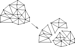
Figure 9.5:
Domain Decomposition of the Finite Element Mesh into Subdomains,
Each of Which are Assigned to Different Hypercube Processors.
The tedious process of specifying the finite-element model to describe
the geometry of the scattering object is greatly simplified by invoking
the graphical editor, PATRAN-Plus, within the Hypercube Electromagnetics
Interactive Analysis Workstation. The graphical input is used to
generate the finite-element mesh. Currently, we have implemented
isoparametric three-node triangular, six-node triangular, and nine-node
quadrilateral elements for the two-dimensional case, and linear four-node
tetrahedral elements for the three-dimensional case.
Once the finite-element mesh has been generated, the elements are
allocated to hypercube processors with the aid of a partitioning tool
which we have developed. In order to achieve good load balance,
each of the hypercube processors should receive approximately
the same number of elements (which reflects the computation load) and
the same number of subdomain edges (which reflects the communication
requirement). The
recursive inertial partitioning
(RIP)
algorithm chooses the best
bisection axis of the mesh based on calculated moments of inertia.
Figure
9.6
illustrates one possible partitioning for a
dielectric cylinder.
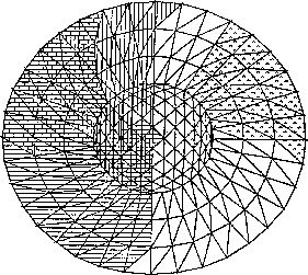
Figure 9.6:
Finite Element Mesh for a Dielectric Cylinder Partitioned Among
Eight Hypercube Processors
The finite-element problem can be solved using several different
strategies: iterative solution, direct solution, or a hybrid of the
two. We employ all of these techniques in our finite elements
testbed. We use a preconditioned biconjugate gradients approach for
iterative solutions and a Crout solver for the direct solution
[Peterson:85d;86a]. We
also have developed a hybrid solver which uses first Gaussian
elimination locally within hypercube processors, and then biconjugate
gradients to resolve the remaining degrees of freedom [
Nour-Omid:87b
].
The output from the finite elements code is displayed graphically at
the Electromagnetics Interactive Analysis Workstation. In Figure 9.7
(Color Plate) are plotted the real (on the left) and the imaginary (on
the right) components of the total scalar field for a conducting
cylinder of
ka=50
. The absorbing boundary is placed at
kr=62
.
Figure 9.8 (Color Plate) shows the plane wave propagation indicated by
vectors in a rectangular box (no scatterer). The box is modeled using
linear tetrahedral elements. Figure 9.9 (Color Plate) shows the plane
wave propagation (no scatterer) in a spherical domain, again using
tetrahedral linear elements. The half slices show the internal
fields. In the upper left is the
x
-component of the field, the lower
left is the
z
-component, and on the right is the
y
-component with
the fields shown as contours on the surface.
Figure 9.7:
Results from the two-dimensional
electromagnetic scalar finite-element code described in the text.
Figure 9.8:
Test case for the electromagnetic
three-dimensional code with no scatterer described in text.
Figure 9.9:
Test case for electromagnetic
three-dimensional planewave in spherical domain with no scatterer describes
in the text.
The speedups over the problem running on one processor are plotted for
hypercube configurations ranging from 1 to 32 processors in
Figure
9.10
. The problem for this set of runs is a
two-dimensional dielectric cylinder model consisting of 9313 nodes.
Figure 9.10:
Finite-Element Execution Speedup Versus Hypercube Size
The setup and solve portions of the total execution time demonstrate
87% and 81% efficiencies, respectively. The output portion where the
results obtained by each processor are sent back to the workstation run
at about 50% efficiency. The input routine exhibits no speedup and
greatly reduces the overall efficiency, 63% of the code. Clearly, this
is an area on which we now must focus. We have recently implemented the
partitioning code on parallel. We are also now reducing the size of the
input file by compressing the contents of the mesh data file and
removing formatted reads and writes. We are also developing a parallel mesh
partitioner which iteratively refines a coarse mesh which was
generated by the graphics software.
We are currently exploring a number of accuracy issues with regards to
the finite elements and coupled approach solutions. Such issues
include gridding density, element types, placement of artificial
boundaries, and specification of basis functions. We are investigating
outgoing wave boundary conditions; currently, we are using a modified
Sommerfield radiation condition in three dimensions. In addition, we
are exploring a number of higher order element types for three
dimensions. Central to our investigations is the objective of
developing analysis techniques for massive three-dimensional problems.
We have demonstrated that the parallel processing environments offered
by the current coarse-grain MIMD architectures are very well suited to
the solution of large-scale electromagnetic scattering and radiation
problems. We have developed a number of parallel EM analysis codes
that currently run in production mode. These codes are being embedded
in a Hypercube Electromagnetic Interactive Analysis Workstation. The
workstation environment simplifies the user specification of the model
geometry and material properties, and the input of run parameters. The
workstation also provides an ideal environment for graphically viewing
the resulting currents and near- and far-fields. We are continuing to
explore a number of issues to fully exploit the capabilities of this
large-memory, high-performance computing environment. We are also
investigating improved matrix solvers for both dense and sparse
matrices, and have implemented out-of-core solving techniques, which
will prevent us from becoming memory-limited. By establishing
testbeds, such as the finite-element one described here, we will
continue to explore issues that will maintain computational accuracy,
while reducing the overall computation time for EM scattering and
radiation analysis problems.
Next:
LU Factorization of
Up:
9 Loosely Synchronous Problems
Previous:
9.3.7 Summary
Guy Robinson
Wed Mar 1 10:19:35 EST 1995
LU Factorization of Sparse, Unsymmetric
Jacobian Matrices
Next:
9.5.1 Introduction
Up:
9 Loosely Synchronous Problems
Previous:
9.4 Computational Electromagnetics
Efficient sparse linear algebra
cannot
be achieved as a
straightforward extension of the dense case described in
Chapter
8
, even for concurrent implementations. This paper
details a new, general-purpose unsymmetric sparse LU
factorization
code built on the
philosophy of Harwell's MA28, with variations. We apply this code in
the framework of Jacobian-matrix factorizations, arising from Newton
iterations in the solution of nonlinear systems of equations. Serious
attention has been paid to the data-structure requirements, complexity
issues, and communication features of the algorithm. Key results
include reduced communication pivoting
for both the
``analyze'' A-mode and repeated B-mode factorizations, and effective
general-purpose data distributions useful incrementally to trade-off
process-column load balance
in factorization
against triangular solve performance. Future planned efforts are
cited in conclusion.
Other References
HPFA Paradigms
Guy Robinson
Wed Mar 1 10:19:35 EST 1995
9.5.1 Introduction
Next:
9.5.2 Design Overview
Up:
LU Factorization of
Previous:
LU Factorization of
The topic of this section is the implementation and concurrent
performance of sparse, unsymmetric LU factorization for medium-grain
multicomputers. Our target hardware is distributed-memory,
message-passing concurrent computers such as the Symult s2010 and
Intel iPSC/2 systems. For both of these systems, efficient cut-through
wormhole
routing technology provides pairwise communication
performance essentially independent of the spatial location of the
computers in the ensemble [
Athas:88a
]. The Symult s2010 is a
two-dimensional, mesh-connected concurrent computer; all examples in
this paper were run on this variety of hardware. Message-passing
performance, portability, and related issues relevant to this work are
detailed in [
Skjellum:90a
].
Figure 9.11:
An Example of Jacobian Matrix Structures. In
chemical-engineering process flowsheets, Jacobians with main-band
structure, lower-triangular structure (feedforwards), upper-triangular
structure (feedbacks), and borders (global or artificially restructured
feedforwards and/or feedbacks) are common.
Questions of linear-algebra performance are pervasive throughout scientific
and engineering computation. The need for high-quality, high-performance
linear algebra algorithms (and libraries) for multicomputer systems therefore
requires no attempt at justification. The motivation for the work described
here has a specific origin, however. Our main higher level research goal is
the concurrent dynamic simulation of systems modelled by ordinary
differential and algebraic equations; specifically, dynamic flowsheet
simulation of chemical plants (e.g., coupled distillation columns)
[
Skjellum:90c
]. Efficient sequential integration algorithms solve
staticized nonlinear equations at each time point via modified Newton
iteration (cf., [
Brenan:89a
], Chapter 5). Consequently, a
sequence of structurally identical linear systems must be solved; the
matrices are finite-difference approximations to
Jacobians
of the staticized system of ordinary
differential-algebraic equations.
These Jacobians are large, sparse, and unsymmetric for our
application area. In general, they possess both band and significant
off-band structure. Generic structures are depicted in
Figure
9.11
. This work should also bear relevance to
electric power network/grid dynamic simulation where sparse,
unsymmetric Jacobians arise, and elsewhere.
Next:
9.5.2 Design Overview
Up:
LU Factorization of
Previous:
LU Factorization of
Guy Robinson
Wed Mar 1 10:19:35 EST 1995
9.5.2 Design Overview
Next:
9.5.3 Reduced-Communication Pivoting
Up:
LU Factorization of
Previous:
9.5.1 Introduction
Figure 9.12:
Process-Grid Data Distribution of
Ax=b
. Representation of a
concurrent matrix, and distributed-replicated concurrent vectors on a
 logical process grid. The solution of
Ax=b
first appears in
x
, a column-distributed vector, and then is normally ``transposed'' via a
global
combine
to the row-distributed vector
y
.
logical process grid. The solution of
Ax=b
first appears in
x
, a column-distributed vector, and then is normally ``transposed'' via a
global
combine
to the row-distributed vector
y
.
We solve the problem
Ax=b
where
A
is large, and includes many zero
entries. We assume that
A
is unsymmetric both in sparsity pattern and in
numerical values. In general, the matrix
A
will be computed in a
distributed fashion, so we will inherit a distribution of the coefficients of
A
(cf., Figures
9.12
and
9.13
).
Following the style of Harwell's MA28 code for unsymmetric sparse
matrices, we use a two-phase approach to this solution. There is a first LU
factorization called A-mode or ``analyze,'' which builds data structures
dynamically, and employs a user-defined pivoting function. The repeated B-mode
factorization uses the existing data structures statically to factor a new,
similarly structured matrix, with the previous pivoting pattern. B-mode
monitors stability with a simple growth factor estimate. In practice, A-mode
is repeated whenever instability is detected. The two key contributions of
this sparse concurrent solver are reduced communication pivoting, and new
data distributions for better overall performance.
Figure 9.13:
Example of Process-Grid Data Distribution. An  array
with block-linear rows (
B=2
) and scattered columns on a
array
with block-linear rows (
B=2
) and scattered columns on a  logical process grid. Local arrays are denoted at left by
  where
where
 is the grid position of the process on
  . Subscripts
(i.e.,
. Subscripts
(i.e.,  ) are the global (
I,J
) indices.
) are the global (
I,J
) indices.
Following Van de Velde [
Velde:90a
], we consider the LU factorization of
a real matrix
A
,  . It is well known (e.g.,
[
Golub:89a
], pp. 117-118), that for any such matrix
A
, an LU
factorization of the form
. It is well known (e.g.,
[
Golub:89a
], pp. 117-118), that for any such matrix
A
, an LU
factorization of the form

exists, where  are square, (orthogonal) permutation
matrices, and
are square, (orthogonal) permutation
matrices, and  are the unit lower- and
upper-triangular factors, respectively. Whereas the pivot sequence is
stored (two
N
-length integer vectors), the permutation matrices are not
stored or computed with explicitly. Rearranging, based on the orthogonality
of the permutation matrices,
are the unit lower- and
upper-triangular factors, respectively. Whereas the pivot sequence is
stored (two
N
-length integer vectors), the permutation matrices are not
stored or computed with explicitly. Rearranging, based on the orthogonality
of the permutation matrices,  We factor
A
with implicit pivoting (no rows or columns are exchanged
explicitly as a result of pivoting). Therefore, we do not store
We factor
A
with implicit pivoting (no rows or columns are exchanged
explicitly as a result of pivoting). Therefore, we do not store  directly, but instead:
 . Consequently,
  ,
,  , and
, and
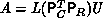 . The ``unravelling'' of the permutation
matrices is accomplished readily (without implication of additional
interprocess communication) during the triangular solves.
. The ``unravelling'' of the permutation
matrices is accomplished readily (without implication of additional
interprocess communication) during the triangular solves.
For the sparse case, performance is more difficult to quantify than for
the dense case, but, for example, banded matrices
with
bandwidth
 can be factored with
  work; we expect subcubic complexity in
N
for reasonably sparse
matrices, and strive for subquadratic complexity, for very sparse
matrices. The triangular solves can be accomplished in work
proportional to the number of entries in the respective triangular
matrix
L
or
U
. The pivoting strategy is treated as a parameter of
the algorithm and is not predetermined. We can consequently treat
the pivoting function as an application-dependent function, and
sometimes tailor it to special problem structures (cf., Section 7 of
[
Velde:88a
]) for higher performance. As for all sparse
solvers, we also seek subquadratic memory requirements in
N
,
attained by storing matrix entries in linked-list fashion, as
illustrated in Figure
9.14
.
work; we expect subcubic complexity in
N
for reasonably sparse
matrices, and strive for subquadratic complexity, for very sparse
matrices. The triangular solves can be accomplished in work
proportional to the number of entries in the respective triangular
matrix
L
or
U
. The pivoting strategy is treated as a parameter of
the algorithm and is not predetermined. We can consequently treat
the pivoting function as an application-dependent function, and
sometimes tailor it to special problem structures (cf., Section 7 of
[
Velde:88a
]) for higher performance. As for all sparse
solvers, we also seek subquadratic memory requirements in
N
,
attained by storing matrix entries in linked-list fashion, as
illustrated in Figure
9.14
.
Figure 9.14:
Linked-list Entry Structure of Sparse Matrix. A single entry
consists of a double-precision value (8 bytes), the local row (i) and column
(j) index (2 bytes each), a ``Next Column Pointer'' indicating the next
current column entry (fixed j), and a ``Next Row Pointer'' indicating the next
current row entry (fixed i), at 4 bytes each. Total: 24 bytes per entry.
For further discussion of LU factorizations and sparse matrices,
see [
Golub:89a
], [
Duff:86a
].
Next:
9.5.3 Reduced-Communication Pivoting
Up:
LU Factorization of
Previous:
9.5.1 Introduction
Guy Robinson
Wed Mar 1 10:19:35 EST 1995
9.5.3 Reduced-Communication Pivoting
Next:
9.5.4 New Data Distributions
Up:
LU Factorization of
Previous:
9.5.2 Design Overview
At each stage of the concurrent LU factorization, the pivot element is
chosen by the user-defined pivot function. Then, the pivot row (new
row of
U
) must be broadcast,
and pivot column (new
column of
L
) must be computed and broadcast
on the
logical process grid (cf., Figure
9.12
), vertically
and horizontally, respectively. Note that these are interchangeable
operations. We use this degree of freedom to reduce the communication
complexity of particular pivoting
strategies, while
impacting the effort of the LU factorization itself negligibly.
We define two ``correctness modes'' of pivoting functions. In the first
correctness mode, ``first row fanout,'' the exit conditions for the pivot
function are: All processes must know  (the pivot process row); the
pivot process row must know
(the pivot process row); the
pivot process row must know  (the pivot process column) as well as
 , the
, the  -local matrix row of the pivot; and the pivot
process must know in addition the pivot value and
-local matrix row of the pivot; and the pivot
process must know in addition the pivot value and  -local matrix
column
-local matrix
column  of the pivot. Partial column pivoting and preset
pivoting can be set up to satisfy these correctness conditions as follows. For
partial column pivoting, the
k
row is eliminated at the
k
step of
the factorization. From this fact, each process can derive the process row
of the pivot. Partial column pivoting and preset
pivoting can be set up to satisfy these correctness conditions as follows. For
partial column pivoting, the
k
row is eliminated at the
k
step of
the factorization. From this fact, each process can derive the process row
 and
and  -local matrix row
  using the row data
distribution function. Having identified themselves, the pivot-row processes
can look for the largest element in local matrix row
using the row data
distribution function. Having identified themselves, the pivot-row processes
can look for the largest element in local matrix row  and choose
the pivot element globally among themselves via a combine. At
completion, this places
and choose
the pivot element globally among themselves via a combine. At
completion, this places  ,
,  , and the pivot value in the
entire pivot process row. This completes the requirements for the ``first row
fanout'' correctness mode. For preset pivoting, the
k
elimination row
and column are both stored as
, and the pivot value in the
entire pivot process row. This completes the requirements for the ``first row
fanout'' correctness mode. For preset pivoting, the
k
elimination row
and column are both stored as  , and
each process knows these values
without communication
.
Furthermore, the pivot process looks up the
pivot value. Hence, preset pivoting satisfies the requirements of this
correctness mode also.
, and
each process knows these values
without communication
.
Furthermore, the pivot process looks up the
pivot value. Hence, preset pivoting satisfies the requirements of this
correctness mode also.
For ``first row fanout,'' the universal knowledge of  and
knowledge of the pivot matrix row
and
knowledge of the pivot matrix row  by the pivot process
row, allow the vertical broadcast
of this row (new
row of
U
). In addition, we broadcast
by the pivot process
row, allow the vertical broadcast
of this row (new
row of
U
). In addition, we broadcast
 ,
,
 , and the pivot value simultaneously. This extends the
correct value of
, and the pivot value simultaneously. This extends the
correct value of  to all processes, as well as
  and
the pivot value to the pivot process column. Hence, the multiplier
(
L
) column may be correctly computed and broadcast
.
Along with the multiplier column broadcast
, we include
the pivot value. After this broadcast
, all processes
have the correct indices
and
the pivot value to the pivot process column. Hence, the multiplier
(
L
) column may be correctly computed and broadcast
.
Along with the multiplier column broadcast
, we include
the pivot value. After this broadcast
, all processes
have the correct indices  and
the pivot value. This provides all that's required to complete the
current elimination step.
and
the pivot value. This provides all that's required to complete the
current elimination step.
For the second correctness mode ``first column fanout,'' the exit conditions
for the pivot function are: All processes must know  and the entire
pivot process column must know
and the entire
pivot process column must know  , the pivot value, and
  .
The pivot process in addition knows
.
The pivot process in addition knows  . Partial row pivoting can
be set up to satisfy these correctness conditions. The arguments are
analogous to partial column pivoting and are given in [
Skjellum:90c
].
. Partial row pivoting can
be set up to satisfy these correctness conditions. The arguments are
analogous to partial column pivoting and are given in [
Skjellum:90c
].
For ``first column fanout,'' the entire pivot process column knows the
pivot value, and local column of the pivot. Hence, the multiplier
column may be computed by dividing the pivot matrix column by the pivot
value. This column of
L
can then be broadcast
horizontally, including the pivot value,  , and
, and  as
additional information. After this step, the entire ensemble has the
correct pivot value, and
as
additional information. After this step, the entire ensemble has the
correct pivot value, and  ; in addition, the pivot process row
has the correct
; in addition, the pivot process row
has the correct  . Hence, the pivot matrix row may be
identified and broadcast
. This second
broadcast
completes the needed information in each
process for effecting the
k
elimination step.
. Hence, the pivot matrix row may be
identified and broadcast
. This second
broadcast
completes the needed information in each
process for effecting the
k
elimination step.
Thus, when using partial row or partial column pivoting, only local
combines of the pivot process column (respectively row) are needed.
The other processes don't participate in the combine, as they must
without this methodology. Preset pivoting implies no pivoting
communication, except very occasionally (e.g., 1 in 5000 times),
as noted in [
Skjellum:90c
], to remove memory unscalabilities. This
pivoting approach is a direct savings, gained at a negligible
additional broadcast
overhead. See also
[
Skjellum:90c
].
Next:
9.5.4 New Data Distributions
Up:
LU Factorization of
Previous:
9.5.2 Design Overview
Guy Robinson
Wed Mar 1 10:19:35 EST 1995
9.5.4 New Data Distributions
Next:
9.5.5 Performance Versus Scattering
Up:
LU Factorization of
Previous:
9.5.3 Reduced-Communication Pivoting
We introduce new closed-form  -time,
  -memory data
distributions
useful for sparse matrix
factorizations and the problems that generate
such matrices. We quantify evaluation costs in Table
9.3
.
-memory data
distributions
useful for sparse matrix
factorizations and the problems that generate
such matrices. We quantify evaluation costs in Table
9.3
.
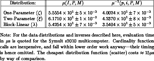
Table 9.3:
Evaluation Times for Three Data Distributions
Every concurrent data structure is associated with a logical process grid at
creation (cf., Figure
9.12
and [Skjellum:90a;90c]).
Vectors are either row- or column-distributed within a
two-dimensional process grid. Row-distributed vectors are
replicated
in each process column, and distributed in the process rows. Conversely,
column-distributed vectors are replicated in each process row, and
distributed in the process columns. Matrices are distributed both in rows
and columns, so that a single process owns a subset of matrix rows and
columns. This partitioning follows the ideas proposed by Fox et al.
[
Fox:88a
] and others. Within the process grid, coefficients of vectors
and matrices are distributed according to one of several data distributions.
Data distributions are chosen to compromise between load-balancing
requirements and constraints on where information can be calculated in the
ensemble.
Definition 1 (Data-Distribution Function)
A data-distribution function  maps three integers
  where
where  , is the global name of a coefficient,
P
is
the number of processes among which all coefficients are to be partitioned,
and
M
is the total number of coefficients. The pair
, is the global name of a coefficient,
P
is
the number of processes among which all coefficients are to be partitioned,
and
M
is the total number of coefficients. The pair  represents the
process
p
(
represents the
process
p
( ) and local (process-
p
) name
i
of the
coefficient (
) and local (process-
p
) name
i
of the
coefficient ( ). The inverse distribution
function
). The inverse distribution
function  transforms the local name
i
back
to the global coefficient name
I
.
transforms the local name
i
back
to the global coefficient name
I
.
The formal requirements for a data-distribution function are as follows. Let
 be the set of global coefficient names associated with process
 , defined implicitly by a data distribution function
 . The following set properties must hold:
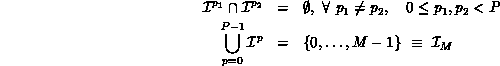
The cardinality of the set  , is given by
  .
.
The linear and scatter data-distribution functions are most often
defined. We generalize these functions (by blocking
and scattering parameters) to incorporate practically important
degrees of freedom. These generalized distribution functions yield
optimal static load balance
as do the unmodified
functions described in [
Velde:90a
] for unit block size, but they
differ in coefficient placement. This distinction is technical, but
necessary for efficient implementations.
Definition 2 (Generalized Block-Linear)
The definitions for the generalized block-linear distribution function,
inverse, and cardinality function are:
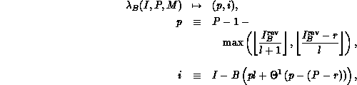
while
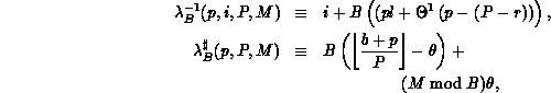
where
B
denotes the coefficient block size,
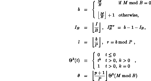
and where  .
.
For
B=1
, a load-balance-equivalent variant of the common linear
data-distribution function is recovered. The general block-linear
distribution function divides coefficients among the
P
processes
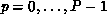 so that each
  is a set of coefficients with
contiguous global names, while optimally load-balancing the
b
blocks among
the
P
sets. Coefficient boundaries between processes are on multiples of
B
. The maximum possible coefficient imbalance between processes is
B
.
If
is a set of coefficients with
contiguous global names, while optimally load-balancing the
b
blocks among
the
P
sets. Coefficient boundaries between processes are on multiples of
B
. The maximum possible coefficient imbalance between processes is
B
.
If  , the last block in process
P-1
will be foreshortened.
, the last block in process
P-1
will be foreshortened.
Definition 3 (Parametric Functions)
To allow greater freedom in the distribution of coefficients among
processes, we define a new, two-parameter distribution function family,
 . The
B
blocking
parameter (just introduced in
the block-linear function) is mainly suited to the clustering of
coefficients that must not be separated by an interprocess boundary
(again, see [
Skjellum:90c
] for a definition of general
block-scatter,
. The
B
blocking
parameter (just introduced in
the block-linear function) is mainly suited to the clustering of
coefficients that must not be separated by an interprocess boundary
(again, see [
Skjellum:90c
] for a definition of general
block-scatter,  ). Increasing
B
worsens the static load
balance. Adding a second scaling parameter
S
(of no impact on the
static load balance) allows the distribution to scatter coefficients to
a greater or lesser degree, directly as a function of this one
parameter. The two-parameter distribution function, inverse and
cardinality function are defined below. The one-parameter distribution
function family,
). Increasing
B
worsens the static load
balance. Adding a second scaling parameter
S
(of no impact on the
static load balance) allows the distribution to scatter coefficients to
a greater or lesser degree, directly as a function of this one
parameter. The two-parameter distribution function, inverse and
cardinality function are defined below. The one-parameter distribution
function family,  , occurs as the special case
B=1
, also as
noted below:
, occurs as the special case
B=1
, also as
noted below:

where
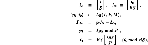
with
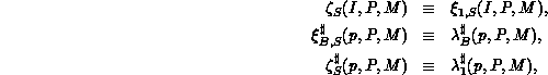
and where
r
,
b
,
etc.
are as defined above.
The inverse distribution function  is defined as
follows:
is defined as
follows:
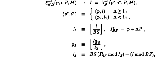
with

For
S = 1
, a block-scatter distribution results, while for  , the generalized block-linear distribution
function is recovered. See also [
Skjellum:90c
].
, the generalized block-linear distribution
function is recovered. See also [
Skjellum:90c
].
Definition 4 (Data Distributions)
Given a data-distribution function family  (
( ), a process list of
P
(
Q
),
M
(
N
) as the number of coefficients, and a row (respectively,
column) orientation, a row (column) data distribution
), a process list of
P
(
Q
),
M
(
N
) as the number of coefficients, and a row (respectively,
column) orientation, a row (column) data distribution  (
( ) is defined as:

respectively,

A two-dimensional data distribution may be identified as consisting of a row
and column distribution defined over a two-dimensional process grid of
 processes, as
  .
.
Further discussion and detailed comparisons on data-distribution functions
are offered in [
Skjellum:90c
]. Figure
9.13
illustrates the
effects of linear and scatter data-distribution functions on a small
rectangular array of coefficients.
Next:
9.5.5 Performance Versus Scattering
Up:
LU Factorization of
Previous:
9.5.3 Reduced-Communication Pivoting
Guy Robinson
Wed Mar 1 10:19:35 EST 1995
9.5.5 Performance Versus Scattering
Next:
9.5.6 Performance
Up:
LU Factorization of
Previous:
9.5.4 New Data Distributions
Consider a fixed logical process grid of
R
processes, with  .
For the sake of argument, assume partial row pivoting during LU factorization
for the retention of numerical stability. Then, for the LU factorization, it
is well known that a scatter distribution is ``good'' for the matrix rows,
and optimal if no off-diagonal pivots were chosen. Furthermore, the
optimal column distribution is also scatter, because columns are chosen in
order for partial row pivoting. Compatibly, a scatter distribution of matrix
rows is also ``good'' for the triangular solves. However, for triangular
solves, the best column distribution is linear, because this implies less
intercolumn communication, as we detail below. In short, the optimal
configurations conflict, and because explicit redistribution is expensive, a
static compromise must be chosen. We address this need to compromise through
the one-parameter distribution function,
.
For the sake of argument, assume partial row pivoting during LU factorization
for the retention of numerical stability. Then, for the LU factorization, it
is well known that a scatter distribution is ``good'' for the matrix rows,
and optimal if no off-diagonal pivots were chosen. Furthermore, the
optimal column distribution is also scatter, because columns are chosen in
order for partial row pivoting. Compatibly, a scatter distribution of matrix
rows is also ``good'' for the triangular solves. However, for triangular
solves, the best column distribution is linear, because this implies less
intercolumn communication, as we detail below. In short, the optimal
configurations conflict, and because explicit redistribution is expensive, a
static compromise must be chosen. We address this need to compromise through
the one-parameter distribution function,  , described in the previous
section, offering a variable degree of scattering via the
S
-parameter. To
first order, changing
S
does not affect the cost of computing the Jacobian
(assuming columnwise finite-difference computation), because each process
column works independently.
, described in the previous
section, offering a variable degree of scattering via the
S
-parameter. To
first order, changing
S
does not affect the cost of computing the Jacobian
(assuming columnwise finite-difference computation), because each process
column works independently.
It's important to note that triangular solves derive no benefit from
Q > 1
. The standard column-oriented solve keeps one process column active
at any given time. For any column distribution, the updated right-hand-side
vectors are retransmitted
W
times (process column-to-process column) during
the triangular solve-whenever the active process column changes. There are
at least  such transmissions (linear distribution), and
at most
such transmissions (linear distribution), and
at most  transmissions (scatter distribution). The
complexity of this retransmission is
transmissions (scatter distribution). The
complexity of this retransmission is  , representing quadratic work
in
N
for
, representing quadratic work
in
N
for  .
.
Calculation complexity for a sparse triangular solve is proportional to the
number of elements in the triangular matrix, with a low leading coefficient.
Often, there are  with
x < 1
elements in the triangular
matrices, including fill. This operation is then
with
x < 1
elements in the triangular
matrices, including fill. This operation is then  , which is
less than quadratic in
N
. Consequently, for large
W
, the retransmission
step is likely of greater cost than the original calculation. This
retransmission effect constrains the amount of scattering and size of
Q
in
order to have any chance of concurrent speedup in the triangular solves.
, which is
less than quadratic in
N
. Consequently, for large
W
, the retransmission
step is likely of greater cost than the original calculation. This
retransmission effect constrains the amount of scattering and size of
Q
in
order to have any chance of concurrent speedup in the triangular solves.
Using the one-parameter distribution with  implies that
 , so that the retransmission complexity is
  .
Consequently, we can bound the amount of retransmission work by making
S
sufficiently large. Clearly,
.
Consequently, we can bound the amount of retransmission work by making
S
sufficiently large. Clearly,  is a hard upper bound, because
we reach the linear distribution limit at that value of the parameter. We
suggest picking
is a hard upper bound, because
we reach the linear distribution limit at that value of the parameter. We
suggest picking  as a first guess, and
  , more
optimistically. The former choice basically reduces retransmission effort by
an order of magnitude. Both examples in the following section illustrate the
effectiveness of choosing
S
by these heuristics.
, more
optimistically. The former choice basically reduces retransmission effort by
an order of magnitude. Both examples in the following section illustrate the
effectiveness of choosing
S
by these heuristics.
The two-parameter  distribution can be used on the matrix rows to
trade off load balance
in the factorizations and
triangular solves against the amount of (communication) effort needed
to compute the Jacobian. In particular, a greater degree of scattering
can dramatically increase the time required for a Jacobian computation
(depending heavily on the underlying equation structure and problem),
but significantly reduce load imbalance during the linear algebra
steps. The communication overhead caused by multiple process rows
suggests shifting toward smaller
P
and larger
Q
(a squatter grid),
in which case greater concurrency is attained in the Jacobian
computation, and the additional communication previously induced is
then somewhat mitigated. The one-parameter distribution used on the
matrix columns then proves effective in controlling the cost of the
triangular solves by choosing the minimally allowable amount of column
scattering.
distribution can be used on the matrix rows to
trade off load balance
in the factorizations and
triangular solves against the amount of (communication) effort needed
to compute the Jacobian. In particular, a greater degree of scattering
can dramatically increase the time required for a Jacobian computation
(depending heavily on the underlying equation structure and problem),
but significantly reduce load imbalance during the linear algebra
steps. The communication overhead caused by multiple process rows
suggests shifting toward smaller
P
and larger
Q
(a squatter grid),
in which case greater concurrency is attained in the Jacobian
computation, and the additional communication previously induced is
then somewhat mitigated. The one-parameter distribution used on the
matrix columns then proves effective in controlling the cost of the
triangular solves by choosing the minimally allowable amount of column
scattering.
Let's specify make explicit the performance objectives we consider when tuning
S
, and, more generally, when tuning the grid shape  .
In the modified Newton iteration, for instance, a Jacobian
factorization is reused until convergence
slows
unacceptably. An ``LU Factorization
+
Backsolve'' step is followed
by
.
In the modified Newton iteration, for instance, a Jacobian
factorization is reused until convergence
slows
unacceptably. An ``LU Factorization
+
Backsolve'' step is followed
by  ``Forward
+
Backsolves,'' with
``Forward
+
Backsolves,'' with  typically
(and varying dynamically throughout the calculation). Assuming an
averaged
typically
(and varying dynamically throughout the calculation). Assuming an
averaged  , say
, say  (perhaps as large as five
[
Brenan:89a
]), then our first-level performance goal is a
heuristic
minimization of
(perhaps as large as five
[
Brenan:89a
]), then our first-level performance goal is a
heuristic
minimization of

over
S
for fixed
P, Q
.  more heavily weights the reduction
of triangular solve costs versus B-mode factorization than we might at
first have assumed, placing a greater potential gain on the one-parameter
distribution for higher overall performance. We generally want heuristically
to optimize
more heavily weights the reduction
of triangular solve costs versus B-mode factorization than we might at
first have assumed, placing a greater potential gain on the one-parameter
distribution for higher overall performance. We generally want heuristically
to optimize

over
S
,
P
,
Q
,
R
. Then, the possibility of fine-tuning row and
column distributions is important, as is the use of non-power-of-two grid
shapes.
Next:
9.5.6 Performance
Up:
LU Factorization of
Previous:
9.5.4 New Data Distributions
Guy Robinson
Wed Mar 1 10:19:35 EST 1995
9.5.6 Performance
Next:
Order 13040 Example
Up:
LU Factorization of
Previous:
9.5.5 Performance Versus Scattering
Guy Robinson
Wed Mar 1 10:19:35 EST 1995
Order 13040 Example
Next:
Order 2500 Example
Up:
9.5.6 Performance
Previous:
9.5.6 Performance
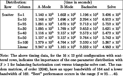
Table 9.4:
Order 13040 Band Matrix Performance
We consider an order 13040 banded matrix
with a
bandwidth
of 326 under partial row pivoting. For this
example, we have compiled timing results for a  process
grid with random matrices (entries have range 0-10,000), using
different values of
S
on the column distribution
(Table
9.4
). We indicate timing for A-mode, B-mode,
Backsolves and Forward- and Backsolves together (``Solve'' heading).
For this example,
S=30
saves
process
grid with random matrices (entries have range 0-10,000), using
different values of
S
on the column distribution
(Table
9.4
). We indicate timing for A-mode, B-mode,
Backsolves and Forward- and Backsolves together (``Solve'' heading).
For this example,
S=30
saves  of the triangular solve cost
compared to
S=1
, or approximately 186 seconds, roughly 6 seconds
above the linear optimal. Simultaneously, we incur about 17 seconds
additional cost in B-mode, while saving about 93 seconds in the
Backsolve. Assuming
of the triangular solve cost
compared to
S=1
, or approximately 186 seconds, roughly 6 seconds
above the linear optimal. Simultaneously, we incur about 17 seconds
additional cost in B-mode, while saving about 93 seconds in the
Backsolve. Assuming 
 , in the first
above-mentioned objective function, we save about 262 (respectively,
76) seconds. Based on this example, and other experiences, we conclude
that this is a successful practical technique for improving overall
sparse linear algebra performance. The following example further
bolsters this conclusion.
, in the first
above-mentioned objective function, we save about 262 (respectively,
76) seconds. Based on this example, and other experiences, we conclude
that this is a successful practical technique for improving overall
sparse linear algebra performance. The following example further
bolsters this conclusion.
Guy Robinson
Wed Mar 1 10:19:35 EST 1995
Order 2500 Example
Next:
9.5.7 Conclusions
Up:
9.5.6 Performance
Previous:
Order 13040 Example
Now, we turn to a timing example of an order 2500 sparse, random matrix. The
matrix has a random diagonal, plus 2 percent random fill of the
off-diagonals; entries have a dynamic range of 0-10,000. Normally, data is
averaged over random matrices for each grid shape (as noted), and over four
repetitive runs for each random matrix. Partial row pivoting was used
exclusively. Table
9.5
compiles timings for various grid shapes
of row-scatter/column-scatter, and row-scatter/column-(
S=10
)
distributions, for as few as nine nodes and as many as 128. Memory
limitations set the lower bound on the number of nodes.
This example demonstrates that speedups are possible for this reasonably
small sparse example with this general-purpose solver, and that the
one-parameter distribution is critical to achieving overall better performance
even for this random, essentially unstructured example. Without the
one-parameter distribution, triangular-solve performance is poor, except in
grid configurations where the factorization is itself degraded (e.g.,
 ). Furthermore, the choice of
S=10
is universally reasonable
for the
Q > 1
grid shapes illustrated here, so the distribution proves easy
to tune for this type of matrix. We are able to maintain an almost constant
speed for the triangular solves while increasing speed for both the A-mode
and B-mode factorizations. We presume, based on experience, that
triangular-solve times are comparable to the sequential solution
times-further study is needed in this area to see if and how
performance can be improved. The consistent A-mode to B-mode ratio of
approximately two is attributed primarily to reduced communication
costs in B-mode, realized through the elimination of essentially all
combine operations in B-mode.
). Furthermore, the choice of
S=10
is universally reasonable
for the
Q > 1
grid shapes illustrated here, so the distribution proves easy
to tune for this type of matrix. We are able to maintain an almost constant
speed for the triangular solves while increasing speed for both the A-mode
and B-mode factorizations. We presume, based on experience, that
triangular-solve times are comparable to the sequential solution
times-further study is needed in this area to see if and how
performance can be improved. The consistent A-mode to B-mode ratio of
approximately two is attributed primarily to reduced communication
costs in B-mode, realized through the elimination of essentially all
combine operations in B-mode.
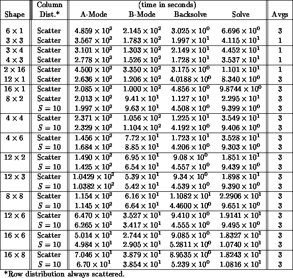
Table 9.5:
Order 2500 Matrix Performance. Performance is a function of grid
shape and size, and
S
-parameter. ``Best'' performance is for the
 grid with
S=10
.
grid with
S=10
.
While triangular-solve performance exemplifies sequentialism in the
algorithm, it should be noted that we do achieve significant overall
performance improvements between 6 nodes and 96 ( grid) nodes,
and that the repeatedly used B-mode factorization remains dominant compared
to the triangular solves even for 128 nodes. Consequently, efforts aimed
at increasing performance of the B-mode factorization (at the expense
of additional A-mode work) are interesting to consider. For the
factorizations, we also expect that we are achieving nontrivial speedups
relative to one node, but we are unable to quantify this at present because
of the memory limitations alluded to above.
grid) nodes,
and that the repeatedly used B-mode factorization remains dominant compared
to the triangular solves even for 128 nodes. Consequently, efforts aimed
at increasing performance of the B-mode factorization (at the expense
of additional A-mode work) are interesting to consider. For the
factorizations, we also expect that we are achieving nontrivial speedups
relative to one node, but we are unable to quantify this at present because
of the memory limitations alluded to above.
Next:
9.5.7 Conclusions
Up:
9.5.6 Performance
Previous:
Order 13040 Example
Guy Robinson
Wed Mar 1 10:19:35 EST 1995
9.5.7 Conclusions
Next:
Concurrent DASSL Applied
Up:
LU Factorization of
Previous:
Order 2500 Example
There are several classes of future work to be considered. First, we
need to take the A-mode ``analyze'' phase to its logical completion, by
including pivot-order sorting of the  pointer structures to
improve performance for systems that should demonstrate subquadratic
sequential complexity. This will require minor modifications to B-mode
(that already takes advantage of column-traversing elimination), to
reduce testing for inactive rows as the elimination progresses. We
already realize optimal computation work in the triangular solves, and
we mitigate the effect of
Q > 1
quadratic communication work using
the one-parameter distribution.
pointer structures to
improve performance for systems that should demonstrate subquadratic
sequential complexity. This will require minor modifications to B-mode
(that already takes advantage of column-traversing elimination), to
reduce testing for inactive rows as the elimination progresses. We
already realize optimal computation work in the triangular solves, and
we mitigate the effect of
Q > 1
quadratic communication work using
the one-parameter distribution.
Second, we need to exploit ``timelike'' concurrency in linear
algebra-multiple pivots. This has been addressed by Alaghband for
shared-memory implementations of MA28 with  -complexity
heuristics [
Alaghband:89a
]. These efforts must be reconsidered in the
multicomputer setting and effective variations must be devised. This
approach should prove an important source of additional speedup for many
chemical engineering
applications, because
of the tendency towards extreme sparsity, with mainly band and/or
block-diagonal structure.
-complexity
heuristics [
Alaghband:89a
]. These efforts must be reconsidered in the
multicomputer setting and effective variations must be devised. This
approach should prove an important source of additional speedup for many
chemical engineering
applications, because
of the tendency towards extreme sparsity, with mainly band and/or
block-diagonal structure.
Third, we could exploit new communication strategies and data
redistribution. Within a process grid, we could incrementally
redistribute  by utilizing the inherent broadcasts of
L
columns
and
U
rows to improve load balance
in the
triangular solves at the expense of slightly more factorization
computational overhead and significantly more memory overhead (a factor
of nearly two). Memory overhead could be reduced at the expense of
further communication if explicit pivoting were used concomitantly.
by utilizing the inherent broadcasts of
L
columns
and
U
rows to improve load balance
in the
triangular solves at the expense of slightly more factorization
computational overhead and significantly more memory overhead (a factor
of nearly two). Memory overhead could be reduced at the expense of
further communication if explicit pivoting were used concomitantly.
Fourth, we can develop adaptive broadcast
algorithms
that track the known load imbalance in the B-mode factorization, and
shift greater communication emphasis to nodes with less computational
work remaining. For example, the pivot column is naturally a ``hot
spot" because the multiplier column (
L
column) must be computed
before broadcast
to the awaiting process columns.
Allowing the non-pivot columns to handle the majority of the
communication could be beneficial, even though this implies additional
overall communication. Similarly, we might likewise apply this to the
pivot row broadcast
, and especially for the pivot
process, because it must participate in two broadcast
operations.
We could utilize two process grids. When rows (columns) of  are
broadcast
, extra broadcasts to a
secondary process grid could reasonably be included. The secondary
process grid could work on redistributing
are
broadcast
, extra broadcasts to a
secondary process grid could reasonably be included. The secondary
process grid could work on redistributing  to an efficient process
grid shape and size for triangular solves while the factorization
continues on the primary grid. This overlapping of communication and
computation could also be used to reduce the cost of transposing the
solution vector from column-distributed to row-distributed, which
normally follows the triangular solves.
to an efficient process
grid shape and size for triangular solves while the factorization
continues on the primary grid. This overlapping of communication and
computation could also be used to reduce the cost of transposing the
solution vector from column-distributed to row-distributed, which
normally follows the triangular solves.
The sparse solver supports arbitrary user-defined pivoting strategies. We
have considered but not fully explored issues of fill-reduction versus
minimum time; in particular we have implemented a Markowitz-count
fill-reduction strategy [
Duff:86a
]. Study of the usefulness of partial
column pivoting and other strategies is also needed. We will report on this
in the future.
Reduced-communication pivoting and parametric distributions can be applied
immediately to concurrent dense solvers with definite improvements in
performance. While triangular solves remain lower-order work in the dense
case, and may sensibly admit less tuning in
S
, the reduction of pivot
communication is certain to improve performance. A new dense solver
exploiting these ideas is under construction at present.
In closing, we suggest that the algorithms generating the sequences of
sparse matrices must themselves be reconsidered in the concurrent setting.
Changes that introduce multiple right-hand sides could help to amortize
linear algebra cost over multiple timelike steps of the higher level
algorithm. Because of inevitable load imbalance, idle processor time is
essentially free-algorithms that find ways to use this time by asking for
more speculative (partial) solutions appear useful in working towards
higher performance.
This work was performed by Anthony Skjellum and Alvin Leung while the
latter held a Caltech Summer Undergraduate Research Fellowship. A
helpful contribution was the dense concurrent linear algebra library
provided by Eric Van de Velde, as well as his prototype sparse
concurrent linear algebra library.
Next:
Concurrent DASSL Applied
Up:
LU Factorization of
Previous:
Order 2500 Example
Guy Robinson
Wed Mar 1 10:19:35 EST 1995
Concurrent DASSL Applied to Dynamic
Distillation Column Simulation
Next:
9.6.1 Introduction
Up:
9 Loosely Synchronous Problems
Previous:
9.5.7 Conclusions
The accurate, high-speed solution of systems of ordinary
differential-algebraic equations (DAEs) of low index is of great
importance in chemical, electrical, and other engineering disciplines.
Petzold's Fortran-based DASSL
is the most widely used
sequential code for solving DAEs. We have devised and implemented a
completely new C code, Concurrent DASSL, specifically for
multicomputers and patterned on DASSL [Skjellum:89a;90c].
In this work, we address
the issues of data distribution and the performance of the overall
algorithm, rather than just that of individual steps. Concurrent DASSL
is designed as an open, application-independent environment below which
linear algebra algorithms may be added in addition to standard support
for dense and sparse algorithms. The user may furthermore attach
explicit data interconversions between the main computational steps, or
choose compromise distributions. A ``problem formulator'' (simulation
layer) must be constructed above Concurrent DASSL, for any specific
problem domain. We indicate performance for a particular chemical
engineering application, a sequence of coupled distillation columns.
Future efforts are cited in conclusion.
Guy Robinson
Wed Mar 1 10:19:35 EST 1995
9.6.1 Introduction
Next:
9.6.2 Mathematical Formulation
Up:
Concurrent DASSL Applied
Previous:
Concurrent DASSL Applied
We discuss the design of a general-purpose integration system
for ordinary differential-algebraic equations
of low index, following up on our more
preliminary discussion in [
Skjellum:89a
]. The new solver,
Concurrent DASSL, is a parallel, C-language implementation of the
algorithm codified in Petzold's DASSL, a widely used Fortran-based
solver for DAE's [
Petzold:83a
], [
Brenan:89a
], and is based on
a loosely synchronous model of communicating sequential processes
[
Hoare:78a
]. Concurrent DASSL retains the same numerical
properties as the sequential algorithm, but introduces important new
degrees of freedom compared to it. We identify the main computational
steps in the integration process; for each of these steps, we specify
algorithms that have correctness independent of data
distribution.
We cover the computational aspects of the major computational steps, and
their data distribution preferences for highest performance. We indicate the
properties of the concurrent sparse linear algebra as it relates to the rest
of the calculation. We describe the proto-Cdyn simulation layer, a
distillation-simulation-oriented Concurrent DASSL driver which,
despite specificity, exposes important requirements for concurrent solution
of ordinary DAE's; the ideas behind a template formulation for simulation
are, for example, expressed.
We indicate formulation issues and specific features of the chemical
engineering problem-dynamic distillation simulation. We indicate
results for an example in this area, which demonstrates not only the
feasibility of this method, but also the need for additional future
work. This is needed both on the sparse linear algebra, and on
modifying the DASSL algorithm to reveal more concurrency, thereby
amortizing the cost of linear algebra over more time steps in the algorithm.
Guy Robinson
Wed Mar 1 10:19:35 EST 1995
9.6.2 Mathematical Formulation
Next:
9.6.3 proto-Cdyn - Simulation
Up:
Concurrent DASSL Applied
Previous:
9.6.1 Introduction
We address the following initial-value problem consisting of combinations of
N
linear and nonlinear coupled, ordinary differential-algebraic
equations over the interval  :
:
IVP
 :
:

with unknown state vector  , known external inputs
 , where
  and
and
 are the given initial-value,
derivative vectors, respectively. We will refer to Equation
9.11
's
deviation from
are the given initial-value,
derivative vectors, respectively. We will refer to Equation
9.11
's
deviation from  as the residuals or residual vector. Evaluating the
residuals means computing
as the residuals or residual vector. Evaluating the
residuals means computing  (``model
evaluation'') for specified arguments
(``model
evaluation'') for specified arguments  ,
,  ,
,  and
t
.
and
t
.
DASSL's integration algorithm can be used to solve systems fully
implicit in  and
and  and of index zero or one, and
specially structured forms of index two (and higher)
[
Brenan:89a
, Chapter 5], where the index is the minimum number of times
that part or all of Equation
9.11
must be differentiated with
respect to
t
in order to express
and of index zero or one, and
specially structured forms of index two (and higher)
[
Brenan:89a
, Chapter 5], where the index is the minimum number of times
that part or all of Equation
9.11
must be differentiated with
respect to
t
in order to express  as a continuous function
of
as a continuous function
of  and
t
[
Brenan:89a
, page 17].
and
t
[
Brenan:89a
, page 17].
By substituting a finite-difference approximation  for
for
 , we obtain:

a set of (in general) nonlinear
staticized
equations. A sequence of
Equation
9.12
's will have to be solved, one at each discrete time
 , in the numerical
approximation scheme; neither
M
nor the
, in the numerical
approximation scheme; neither
M
nor the  's need be
predetermined. In DASSL, the variable step-size integration algorithm
picks the
's need be
predetermined. In DASSL, the variable step-size integration algorithm
picks the  's as the integration progresses, based on its
assessment of the local error. The discretization operator for
's as the integration progresses, based on its
assessment of the local error. The discretization operator for  ,
,  , varies during the numerical integration process and
hence is subscripted as
, varies during the numerical integration process and
hence is subscripted as  .
.
The usual way to solve an instance of the staticized equations,
Equation
9.12
, is via the familiar Newton-Raphson iterative
method (yielding  ):
):

given an initial, sufficiently good approximation  . The
classical method is recovered for
. The
classical method is recovered for  and
c = 1
, whereas a modified
(damped) Newton-Raphson method results for
and
c = 1
, whereas a modified
(damped) Newton-Raphson method results for  (respectively,
 ). In the original DASSL algorithm and in Concurrent
DASSL, the Jacobian
). In the original DASSL algorithm and in Concurrent
DASSL, the Jacobian  is
computed by finite differences
rather than
analytically; this departure leads in another sense to a modified
Newton-Raphson method even though
is
computed by finite differences
rather than
analytically; this departure leads in another sense to a modified
Newton-Raphson method even though  and
c = 1
might always
be satisfied. For termination, a limit
and
c = 1
might always
be satisfied. For termination, a limit  is imposed; a
further stopping criterion of the form
is imposed; a
further stopping criterion of the form  is also incorporated (see Brenan et al.
[
Brenan:89a
, pages 121-124]).
is also incorporated (see Brenan et al.
[
Brenan:89a
, pages 121-124]).
Following Brenan et al., the approximation  is
replaced by a BDF-generated linear approximation,
is
replaced by a BDF-generated linear approximation,  ,
and the Jacobian
,
and the Jacobian

From this approximation, we define  in the intuitive way. We then consider Taylor's Theorem with
remainder, from which we can easily express a forward finite-difference
approximation for each Jacobian column (assuming sufficient smoothness of
in the intuitive way. We then consider Taylor's Theorem with
remainder, from which we can easily express a forward finite-difference
approximation for each Jacobian column (assuming sufficient smoothness of
 ) with a scaled difference of two residual vectors:

By picking  proportional to
  , the
j
unit vector in the natural basis for
, the
j
unit vector in the natural basis for  , namely
 , Equation
9.15
yields a
first-order-accurate approximation in
, Equation
9.15
yields a
first-order-accurate approximation in  of the
j
column of the
Jacobian matrix:
of the
j
column of the
Jacobian matrix:
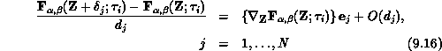
Each of these
N
Jacobian-column computations is independent and
trivially parallelizable. It's well known, however, that for special
structures such as banded
and block
n
-diagonal
matrices, and even for general sparse matrices, a single residual can
be used to generate multiple Jacobian columns [
Brenan:89a
],
[
Duff:86a
]. We discuss these issues as part of the concurrent
formulation section below.
The solution of the Jacobian linear system of equations is required for each
k
-iteration, either through a direct (e.g., LU-factorization) or
iterative (e.g., preconditioned-conjugate-gradient) method. The most
advantageous solution approach depends on
N
as well as special mathematical
properties and/or structure of the Jacobian matrix  . Together, the inner (linear equation solution) and
outer (Newton-Raphson iteration)
loops solve a single
time point; the overall algorithm generates a sequence of solution points
. Together, the inner (linear equation solution) and
outer (Newton-Raphson iteration)
loops solve a single
time point; the overall algorithm generates a sequence of solution points
 .
.
In the present work, we restrict our attention to direct, sparse linear
algebra as described in [
Skjellum:90d
], although future versions of
Concurrent DASSL will support the iterative linear algebra approaches
by Ashby, Lee, Brown, Hindmarsh et al. [
Ashby:90a
],
[
Brown:91a
]. For the sparse LU factorization, the factors are stored
and reused in the modified Newton scenario. Then, repeated use of the old
Jacobian implies just a forward- and back-solve step using the triangular
factors
L
and
U
. Practically, we can use the Jacobian for up to about
five steps [
Brenan:89a
]. The useful lifetime of a single Jacobian
evidently depends somewhat strongly on details of the integration procedure
[
Brenan:89a
].
Next:
9.6.3 proto-Cdyn - Simulation
Up:
Concurrent DASSL Applied
Previous:
9.6.1 Introduction
Guy Robinson
Wed Mar 1 10:19:35 EST 1995
9.6.3 proto-Cdyn - Simulation Layer
Next:
Template Structure
Up:
Concurrent DASSL Applied
Previous:
9.6.2 Mathematical Formulation
To use the Concurrent DASSL system on other than toy problems, a
simulation layer must be constructed above it. The purpose of this layer is
to accept a problem specification from within a specific problem domain, and
formulate that specification for concurrent solution as a set of
differential-algebraic equations, including any needed data. On one hand,
such a layer could explicitly construct the subset of equations needed for
each processor, generate the appropriate code representing the residual
functions, and create a set of node programs for effecting the simulation.
This is the most flexible approach, allowing the user to specify arbitrary
nonlinear DAEs. It has the disadvantage of requiring a lot of compiling and
linking for each run in which the problem is changed in any significant
respect (including but not limited to data distribution), although with
sophisticated tactics, parametric variations within equations could be
permitted without recompiling from scratch, and incremental linking could be
supported.
We utilize a template-based approach here, as we do in the Waveform-Relaxation
paradigm for concurrent dynamic simulation
[
Skjellum:88a
]. This is akin to the
ASCEND II
methodology
utilized by Kuru and many others [
Kuru:81a
]. It is a compromise
approach from the perspective of flexibility; interesting physical
prototype subsystems are encapsulated into compiled code as templates.
A template is a conceptual building block with states, nonstates,
parameters, inputs, and outputs (see below). A general network made
from instantiations of templates can be constructed at run time without
changing any executable code. User input specifies the number and type
of each template, their interconnection pattern, and the initial value
of systemic states and extraneous (nonstate) variables, plus the value
of adjustable parameters and more elaborate data, such as physical
properties. The addition of templates requires new subroutines for the
evaluation of the residuals of their associated DAEs, and for
interfacing to the remainder of the system (e.g., parsing of user
input, interconnectivity issues). With suitable automated tools, this
addition process can be made straightforward to the user.
Importantly, the use of a template-based methodology does not imply a
degradation in the numerical quality of the model equations or solution
method used. We are not obliged to tear equations based on templates
or groups of templates as is done in sequential-modular simulators
[
Westerberg:79a
], [
Cook:80a
], where ``sequential'' refers in this
sense to the stepwise updating of equation subsets, without connection to the
number of computers assigned to the problem solution.
Ideally, the simulation layer could be made universal. That is, a
generic layer of high flexibility and structural elegance would be
created once and for all (and without predilection for a specific
computational engine). Thereafter, appropriate templates would be
added to articulate the simulator for a given problem domain. This is
certainly possible with high-quality simulators such as ASCEND II and
Chemsim (a recent Fortran-based simulator driving DASSL and MA28
[
Andersen:88a
], [
Duff:77a
], [
Petzold:83a
]). Even so, we
have chosen to restrict our efforts to a more modest simulation layer,
called proto-Cdyn, which can create arbitrary networks of coupled
distillation columns. This restricted effort has required significant
effort, and already allows us to explore many of the important issues
of concurrent dynamic simulation. General-purpose simulators are for
future consideration. They must address significant questions of
user-interface in addition to concurrency-formulation issues.
In the next paragraphs, we describe the important features of
proto-Cdyn. In doing so, we indicate important issues for any
Concurrent DASSL driver.
Next:
Template Structure
Up:
Concurrent DASSL Applied
Previous:
9.6.2 Mathematical Formulation
Guy Robinson
Wed Mar 1 10:19:35 EST 1995
Template Structure
Next:
Problem Preformulation
Up:
9.6.3 proto-Cdyn - Simulation
Previous:
9.6.3 proto-Cdyn - Simulation
A template is a prototype for a sequence of DAEs which can be used
repeatedly in different instantiations. Normally, but not always, the
template corresponds to some subsystem of a physical-model description of a
system, like a tank or distillation tray. The key characteristics of a
template are: the number of integration states it incorporates (typically
fixed), the number of nonstate variables it incorporates (typically fixed),
its input and output connections to other templates, and external sources
(forcing functions) and sinks. State variables participate in the overall
DASSL integration process. Nonstates are defined as variables
which, given the states of a template alone, may be computed uniquely. They
are essentially local tear variables. It is up to the template designer
whether or not to use such local tear variables: They impact the numerical
quality of the solution, in principle. Alternative formulations, where all
variables of a template are treated as states, can be posed and comparisons
made. Because of the superlinear growth of linear algebra complexity, the
introduction of extra integration states must be justified on the basis of
numerical accuracy. Otherwise, they artificially slow down the problem
solution, perhaps significantly. Nonstates are extremely convenient and
practically useful; they appear in all the dynamic simulators we have come
across.
The template state and nonstate structure imply a two-phase residual
computation. First, given a state  , the non-states of each template
are updated on a template-by-template basis. Then, given its states and
non-states, inputs from other templates and external inputs, each template's
residuals may be computed. In the sequential implementation, this poses no
particular nuisances, other than having two evaluation loops over all templates.
However, in concurrent evaluation, a communication phase intervenes between
nonstate and residual updates. This communication phase transmits
all states and nonstates appearing as outputs of templates to their
corresponding inputs at other templates. This transmission mechanism is
considered below under concurrent formulation.
, the non-states of each template
are updated on a template-by-template basis. Then, given its states and
non-states, inputs from other templates and external inputs, each template's
residuals may be computed. In the sequential implementation, this poses no
particular nuisances, other than having two evaluation loops over all templates.
However, in concurrent evaluation, a communication phase intervenes between
nonstate and residual updates. This communication phase transmits
all states and nonstates appearing as outputs of templates to their
corresponding inputs at other templates. This transmission mechanism is
considered below under concurrent formulation.
Next:
Problem Preformulation
Up:
9.6.3 proto-Cdyn - Simulation
Previous:
9.6.3 proto-Cdyn - Simulation
Guy Robinson
Wed Mar 1 10:19:35 EST 1995
Problem Preformulation
Next:
9.6.4 Concurrent Formulation
Up:
9.6.3 proto-Cdyn - Simulation
Previous:
Template Structure
In general, the ``optimal'' ordering for the equations of a dynamic
simulation will in general be too difficult to establish
, because
of the NP-hard issues involved in structure selection. However, many
important heuristics can be applied, such as those that precedence-order the
nonlinear equations, and those that permute the Jacobian structure to a more
nearly triangular or banded form [
Duff:86a
]. For the proto-Cdyn
simulator, we skirt these issues entirely, because it proves easy to arrange
a network of columns to produce a ``good structure''-a main block
tridiagonal Jacobian structure with off-block-diagonal structure for the
intercolumn connections, simply by taking the distillation columns with their
states in tray-by-tray, top-down (or bottom-up) order.
Given a set of DAEs, and an ordering for the equations and states
(i.e., rows and columns of the Jacobian, respectively), we need to
partition these equations between the multicomputer nodes, according to a
two-dimensional process grid of shape  . The partitioning of
the equations forms, in main part, the so-called concurrent database.
This grid structure is illustrated in [
Skjellum:90d
, Figure 2.]. In
proto-Cdyn, we utilize a single process grid for the entire
Concurrent DASSL calculation. That is, we do not currently exploit the
Concurrent DASSL feature which allows explicit transformations
between the main calculational phases (see below). In each process column,
the entire set of equations is to be reproduced, so that any process column
can compute not only the entire residual vector for a prediction calculation,
but also, any column of the Jacobian matrix.
. The partitioning of
the equations forms, in main part, the so-called concurrent database.
This grid structure is illustrated in [
Skjellum:90d
, Figure 2.]. In
proto-Cdyn, we utilize a single process grid for the entire
Concurrent DASSL calculation. That is, we do not currently exploit the
Concurrent DASSL feature which allows explicit transformations
between the main calculational phases (see below). In each process column,
the entire set of equations is to be reproduced, so that any process column
can compute not only the entire residual vector for a prediction calculation,
but also, any column of the Jacobian matrix.
A mapping between the global and local equations must be created.
In the general case, it will be difficult to generate a closed-form
expression for either the global-to-local mapping or its inverse (that also
require  storage). At most, we will have on a hand a partial (or
weak) inverse in each process, so that the corresponding global index of each
local index will be available. Furthermore, in each node, a partial
global-to-local list of indices associated with the given node will be stored
in global sort order. Then, by binary search, a weak global-to-local mapping
will be possible in each process. That is, each process will be able to
identify if a global index resides within it, and the corresponding local
index. A strong mapping for row (column) indices will require communication
between all the processes in a process row (respectively, column). In the
foregoing, we make the tacit assumption that it is an unreasonable practice
to use storage proportional to the entire problem size
N
in each node,
except if this unscalability can be removed cheaply when necessary for large
problems.
storage). At most, we will have on a hand a partial (or
weak) inverse in each process, so that the corresponding global index of each
local index will be available. Furthermore, in each node, a partial
global-to-local list of indices associated with the given node will be stored
in global sort order. Then, by binary search, a weak global-to-local mapping
will be possible in each process. That is, each process will be able to
identify if a global index resides within it, and the corresponding local
index. A strong mapping for row (column) indices will require communication
between all the processes in a process row (respectively, column). In the
foregoing, we make the tacit assumption that it is an unreasonable practice
to use storage proportional to the entire problem size
N
in each node,
except if this unscalability can be removed cheaply when necessary for large
problems.
The proto-Cdyn simulator works with templates of specific
structure-each template is a form of a distillation tray and generates the
same number of integration states. It therefore skirts the need for weak
distributions. Consequently, the entire row-mapping procedure can be
accomplished using the closed-form general two-parameter distribution
function family  described in [
Skjellum:90d
], where the block size
B
is chosen as the number of integration states per template. The
column-mapping procedure is accomplished with the one-parameter distribution
function family
described in [
Skjellum:90d
], where the block size
B
is chosen as the number of integration states per template. The
column-mapping procedure is accomplished with the one-parameter distribution
function family  also described in [
Skjellum:90d
]. The effects of
row and column degree-of-scattering are described in [
Skjellum:90d
]
with attention to linear algebra performance.
also described in [
Skjellum:90d
]. The effects of
row and column degree-of-scattering are described in [
Skjellum:90d
]
with attention to linear algebra performance.
Next:
9.6.4 Concurrent Formulation
Up:
9.6.3 proto-Cdyn - Simulation
Previous:
Template Structure
Guy Robinson
Wed Mar 1 10:19:35 EST 1995
9.6.4 Concurrent Formulation
Next:
Overview
Up:
Concurrent DASSL Applied
Previous:
Problem Preformulation
Guy Robinson
Wed Mar 1 10:19:35 EST 1995
Overview
Next:
Single Integration Step
Up:
9.6.4 Concurrent Formulation
Previous:
9.6.4 Concurrent Formulation
Next, we turn to Equation
9.11
's (that is,
IVP
's)
concurrent numerical solution via the DASSL algorithm. We cover the
major computational steps in abstract, and we also describe the generic
aspects of proto-Cdyn in this connection. In the subsequent section,
we discuss issues peculiar to the distillation simulation.
Broadly, the concurrent solution of
IVP
consists of three block
operations: startup, dynamic simulation, and a cleanup phase.
Significant concurrency is apparent only in the dynamic simulation
phase. We will assume that the simulation interval requested generates
enough work so that the startup and cleanup phases prove insignificant
by comparison and consequently pose no serious
Amdahl's-law
bottleneck. Given this assumption, we
can restrict our attention to a single step of
IVP
as illustrated
schematically in Figure
9.15
.
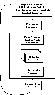
Figure 9.15:
Major Computational Blocks of a Single Integration Step.A single step in the integration begins with a number of BDF-related
computations, including the solution ``prediction'' step. Then,
``correction'' is achieved through Newton iteration steps, each involving a
Jacobian computation, and linear-system solution (LU factorization plus
forward- and back-solves). The computation of the Jacobian in turn relies upon
multiple independent residual calculations, as shown. The three items
enclosed in the rounded rectangle (Jacobian computation-through at most
N
Residual computations-and LU factorization) are, in practice, computed less
often than the others-the old Jacobian matrix is used in the iteration loop
until convergence
slows intolerably.
In the startup phase, a sequential host program interprets the user
specification for the simulation. From this it generates the concurrent
database: the templates and their mutual interconnections, data needed by
particular templates, and a distribution of this information among the
processes that are to participate. The processes are themselves spawned and
fed their respective databases.
Once they receive
their input information, the processes rebuild the data structures for
interfacing with Concurrent DASSL,
and for
generating the residuals. Tolerances and initial derivatives must be
computed and/or estimated. Furthermore, in each process column, the
processes must rendezvous to finalize their communication labelling for
the transmission of states and nonstates to be performed during the
residual calculation. This provides the basis for a reactive,
deadlock-free
update procedure described below.
The cleanup phase basically retrieves appropriate state values and returns
them to the host for propagation to the user. Cleanup may be
interspersed intermittently with the actual dynamic simulation. It provides
a simple record of the results of simulation and terminates the concurrent
processes at the simulation's conclusion.
The dynamic simulation phase consists of repetitive prediction and correction
steps, and marches in time. Each successful time step requires the solution
of one or more instances of Equation
9.12
-additional time steps
that converge but fail to satisfy error tolerances, or fail to converge
quickly enough, are necessarily discarded. In the next section, we cover
aspects of these operations in more detail, for a single step.
Next:
Single Integration Step
Up:
9.6.4 Concurrent Formulation
Previous:
9.6.4 Concurrent Formulation
Guy Robinson
Wed Mar 1 10:19:35 EST 1995
Single Integration Step
Next:
The Integration Computations
Up:
9.6.4 Concurrent Formulation
Previous:
Overview
Guy Robinson
Wed Mar 1 10:19:35 EST 1995
The Integration Computations
Next:
Single Residuals
Up:
Single Integration Step
Previous:
Single Integration Step
These computations of DASSL are a
fixed-leading-coefficient, variable-stepsize and -order,
backward-differentiation-formula (BDF) implicit integration scheme, described
clearly in [
Brenan:89a
, Chapter 5] and outlined in [
Petzold:83a
].
Concurrent DASSL faithfully implements this numerical method, with no
significant differences. Test problems run with the DASSL Fortran
code and the new C code (on one and multiple computers) certify this degree
of compatibility.
The sequential time complexity of the integration computations is  , if
considered separately from the residual calculation called in turn, which is
also normally
, if
considered separately from the residual calculation called in turn, which is
also normally  (see below). We pose these operations on a
 grid, where we assume that each process column can compute
complete residual vectors. Each process column repeats the entire prediction
operations: There is no speedup associated with
Q > 1
, and we replicate
all DASSL BDF and predictor vectors in each process column. Taller,
narrower grids are likely to provide the overall greatest speedup, though the
residual calculation may saturate (and slow down again) because of excessive
vertical communication requirements. It's definitely not true that the
grid, where we assume that each process column can compute
complete residual vectors. Each process column repeats the entire prediction
operations: There is no speedup associated with
Q > 1
, and we replicate
all DASSL BDF and predictor vectors in each process column. Taller,
narrower grids are likely to provide the overall greatest speedup, though the
residual calculation may saturate (and slow down again) because of excessive
vertical communication requirements. It's definitely not true that the
 shape is optimal in all cases.
The distribution of coefficients in the rows has no impact on the integration
operations, and is dictated largely by the requirements of the residual
calculation itself. In practical problems, the concurrent database cannot be
reproduced in each process (cf., [
Lorenz:92a
]), so a given process
will only be able to compute some of the residuals. Furthermore, we may not
have complete freedom in scattering these equations, because there will often
be a trade-off between the degree of scattering and the amount of
communication needed to form the entire residual vector.
The amount of  integration-computation work is not terribly
large-there is consequently a nontrivial but not tremendous effort
involved in the integration computations. (Residual computations
dominate in many if not most circumstances.) Integration operations
consist mainly of vector-vector operations not requiring any
interprocess communication and, in addition, fixed startup costs.
Operations include prediction of the solution at the time point,
initiation and control of the Newton iteration that ``corrects'' the
solution, convergence
and error-tolerance checking,
and so forth. For example, the approximation
integration-computation work is not terribly
large-there is consequently a nontrivial but not tremendous effort
involved in the integration computations. (Residual computations
dominate in many if not most circumstances.) Integration operations
consist mainly of vector-vector operations not requiring any
interprocess communication and, in addition, fixed startup costs.
Operations include prediction of the solution at the time point,
initiation and control of the Newton iteration that ``corrects'' the
solution, convergence
and error-tolerance checking,
and so forth. For example, the approximation  is chosen
within this block using the BDF formulas. For these operations, each
process column currently operates independently, and repetitively forms
the results. Alternatively, each process column could stride with step
Q
, and row-combines could be used to propagate information
across the columns [
Skjellum:90a
]. This alternative would
increase speed for sufficiently large problems, and can easily be
implemented. However, because of load imbalance in other stages of the
calculation, we are convinced that including this type of
synchronization could be an overall negative rather than positive to
performance. This alternative will nevertheless be a future
user-selectable option.
is chosen
within this block using the BDF formulas. For these operations, each
process column currently operates independently, and repetitively forms
the results. Alternatively, each process column could stride with step
Q
, and row-combines could be used to propagate information
across the columns [
Skjellum:90a
]. This alternative would
increase speed for sufficiently large problems, and can easily be
implemented. However, because of load imbalance in other stages of the
calculation, we are convinced that including this type of
synchronization could be an overall negative rather than positive to
performance. This alternative will nevertheless be a future
user-selectable option.
Included in these operations are a handful of norm operations, which
constitute the main interprocess communication required by the
integration computations step; norms are implemented concurrently via
recursive doubling (combine) [
Stone:87a
], [
Skjellum:90a
].
Actually, the weighted norm used by DASSL requires two recursive
doubling operations, each of which combines a scalar. The first
operation obtains the vector coefficient of maximum absolute value, the
second sums the weighted norm itself. Each can be implemented as
Q
independent column combines, each producing the same repetitive result,
or a single
Q
-striding norm that takes advantage of the repetition of
information, but utilizes two combines over the entire process grid.
Both are supported in Concurrent DASSL, although the former is the
default norm. As with the original DASSL, the norm function can be
replaced, if desired.
Next:
Single Residuals
Up:
Single Integration Step
Previous:
Single Integration Step
Guy Robinson
Wed Mar 1 10:19:35 EST 1995
Single Residuals
Next:
Jacobian Computation
Up:
Single Integration Step
Previous:
The Integration Computations
These are computed in prediction and as needed
during correction. Multiple residuals are computed when forming the
finite-difference Jacobian. Single residuals are computed repetitively in
each process column, whereas the multiple residuals of a Jacobian computation
are computed uniquely in the process columns.
Here, we consider the single residual computation required by the integration
computations just described. Given a state vector  , and
approximation for
, and
approximation for  , we need to evaluate
 . The exploitable concurrency available in this step is strictly
a function of the model equations. As defined, there are
N
equations in
this system, so we expect to use at best
N
computers for this step.
Practically, there will be interprocess communication between the process
rows, corresponding to the connectivity among the equations. This will place
an upper limit on
. The exploitable concurrency available in this step is strictly
a function of the model equations. As defined, there are
N
equations in
this system, so we expect to use at best
N
computers for this step.
Practically, there will be interprocess communication between the process
rows, corresponding to the connectivity among the equations. This will place
an upper limit on  (the number of row processes) that can be used
before the speed will again decrease: We can expect efficient speedup for
this step provided that the cost of the interprocess communication is
insignificant compared to the single-equation grain size. As estimated in
[
Skjellum:90a
], the granularity
(the number of row processes) that can be used
before the speed will again decrease: We can expect efficient speedup for
this step provided that the cost of the interprocess communication is
insignificant compared to the single-equation grain size. As estimated in
[
Skjellum:90a
], the granularity  for the
Symult s2010 multicomputer is about fifty, so this implies about 450
floating-point operations per communication in order to achieve
90% concurrent efficiency in this phase.
for the
Symult s2010 multicomputer is about fifty, so this implies about 450
floating-point operations per communication in order to achieve
90% concurrent efficiency in this phase.
Guy Robinson
Wed Mar 1 10:19:35 EST 1995
Jacobian Computation
Next:
Exploitation of Latency
Up:
Single Integration Step
Previous:
Single Residuals
There is evidently much more available
concurrency in this computational step than for the single residual and
integration operations, since, for finite differencing,
N
independent
residual computations are apparently required, each of which is a
single-state perturbation of  . Based on our overview of the
residual computation, we might naively expect to use
. Based on our overview of the
residual computation, we might naively expect to use  processes
effectively; however, the simple perturbations can actually require much
less model evaluation effort because of latency
[
Duff:86a
], [
Kuru:81a
], which is directly a function of the
sparsity structure of the model equations as seen in,
Equation
9.11
. In short, we can attain the same
performance with much less than
processes
effectively; however, the simple perturbations can actually require much
less model evaluation effort because of latency
[
Duff:86a
], [
Kuru:81a
], which is directly a function of the
sparsity structure of the model equations as seen in,
Equation
9.11
. In short, we can attain the same
performance with much less than  processors.
In general, we'd like to consider the Jacobian computation on a rectangular
grid. For this, we can consider using  to accomplish the
calculation. With a general grid shape, we exploit some concurrency in
both
the column evaluations and the residual computations, with
to accomplish the
calculation. With a general grid shape, we exploit some concurrency in
both
the column evaluations and the residual computations, with
 the time for this step,
 the corresponding speedup,
  the
residual evaluation time with
P
row processes, and
the
residual evaluation time with
P
row processes, and  the
apparent speedup compared to one row process:
the
apparent speedup compared to one row process:
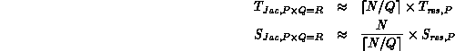
assuming no shortcuts are available as a result of latency. This timing is
exemplified in the example below, which does not take advantage of latency.
There is additional work whenever the Jacobian structure is rebuilt for
better numerical stability in the subsequent LU factorization (A-mode).
Then,  work is involved in each process in the filling of the
initial Jacobian. In the normal case, work proportional to the number of
local nonzeroes plus fill elements is incurred in each process for
refilling the sparse Jacobian structure.
work is involved in each process in the filling of the
initial Jacobian. In the normal case, work proportional to the number of
local nonzeroes plus fill elements is incurred in each process for
refilling the sparse Jacobian structure.
Guy Robinson
Wed Mar 1 10:19:35 EST 1995
Exploitation of Latency
Next:
The LU Factorization
Up:
Single Integration Step
Previous:
Jacobian Computation
This approach has
been considered in the Concurrent DASSL framework. We currently have
experimental versions of two mechanisms, both of which are designed to
work with the sparse-matrix structures associated with direct, sparse
LU factorization ([
Skjellum:90d
]). The first is called
``bandlike'' Jacobian evaluation. For a banded Jacobian matrix of
bandwidth
b
, only
b
residuals are needed to
evaluate the Jacobian. This feature is incorporated into the original
DASSL, along with a LINPACK banded solver. In Concurrent DASSL,
collections of Jacobian columns are placed in each process column,
according to the column data distribution, which thus far is picked
solely to balance LU factorization and triangular-solve performance
[
Skjellum:90d
]. In each process column, there will be
``compatible'' columns that can be evaluated using a single, composite
perturbation. Identification of these compatible columns is
accomplished by checks on the bandwidth
overlap
condition. Columns that possess off-band structure are stricken from
the list and evaluated separately. Presumably, a heuristic algorithm
could be employed further to increase the size of the compatible sets,
but this is yet to be implemented. The same ``greedy'' algorithm of
Curtis et al. used for the sequential reduction of Jacobian computation
effort would be applied independently to each process column (see
comments by [
Duff:86a
, Section 12.3]). Then, clearly, the column
distribution affects the performance of the Jacobian computation, and
the linear-algebra performance can no longer be viewed so readily in
isolation.
We have also devised a ``blocklike'' format, which will be applied to block
n-diagonal matrices that include some off-block entries as well. Optimally,
fewer residual computations will be needed than for the banded case. The same
column-by-column compatible sets will be created, and the Curtis algorithm
can also be applied. Hopefully, because of the less restrictive
compatibility requirement, the blocklike case will produce higher
concurrent speedups than those attained using the conservative bandlike
assumption for Jacobians possessing blocklike structure. Comparative results
will be presented in a future paper.
Next:
The LU Factorization
Up:
Single Integration Step
Previous:
Jacobian Computation
Guy Robinson
Wed Mar 1 10:19:35 EST 1995
The LU Factorization
Next:
Forward- and Back-solving
Up:
Single Integration Step
Previous:
Exploitation of Latency
Following the philosophy of Harwell's MA28, we have interfaced a new
concurrent sparse solver to Concurrent DASSL, the details of which are
quoted elsewhere in this proceedings [
Skjellum:90d
]. In short,
there is a two-step factorization procedure: A-mode, which chooses
stable pivots according to a user-specified function, and builds the
sparse data structures dynamically; and B-mode, which reuses the data
structures and pivot sequence on a similar matrix, but monitors
stability with a growth-factor test. A-mode is repeated whenever
necessary to avoid instability. We expect subcubic time complexity and
subquadratic space complexity in
N
for the sparse solver. We attain
acceptable factorization speedups for systems that are not narrow
banded, and of sufficient size. We intend to incorporate multiple
pivoting heuristic strategies, following [
Alaghband:89a
], to
further improve performance of future versions of the solver. This may
also contribute to better performance of the triangular solves.
Guy Robinson
Wed Mar 1 10:19:35 EST 1995
Forward- and Back-solving Steps
Next:
Residual Communication
Up:
Single Integration Step
Previous:
The LU Factorization
These take the factored
form  , with
  unit lower-triangular,
  upper-triangular, and permutation
matrices
upper-triangular, and permutation
matrices  ,
,  , and solve
Ax = b
, using the
implicit pivoting approach described in [
Skjellum:90d
].
Sequentially, the triangular solves each require work proportional to
the number of entries in the respective triangular factor, including
fill-in. We have yet to find an example of sufficient size for which
we actually attain speedup for these operations, at least for the
sparse case. At most, we try to prevent these operations from becoming
competitive in cost to the B-mode factorization; we detail these
efforts in [
Skjellum:90d
]. In brief, the optimum grid shape for
the triangular solves has
Q=1
, and
P
somewhat reduced from what we
can use in all the other steps. As stated,
P
small seems better thus
far, although for many examples increasing the overhead as a function
of increasing
P
is not unacceptable (see [
Skjellum:90d
] and the
example below).
, and solve
Ax = b
, using the
implicit pivoting approach described in [
Skjellum:90d
].
Sequentially, the triangular solves each require work proportional to
the number of entries in the respective triangular factor, including
fill-in. We have yet to find an example of sufficient size for which
we actually attain speedup for these operations, at least for the
sparse case. At most, we try to prevent these operations from becoming
competitive in cost to the B-mode factorization; we detail these
efforts in [
Skjellum:90d
]. In brief, the optimum grid shape for
the triangular solves has
Q=1
, and
P
somewhat reduced from what we
can use in all the other steps. As stated,
P
small seems better thus
far, although for many examples increasing the overhead as a function
of increasing
P
is not unacceptable (see [
Skjellum:90d
] and the
example below).
Guy Robinson
Wed Mar 1 10:19:35 EST 1995
Residual Communication
Next:
9.6.5 Chemical Engineering Example
Up:
Single Integration Step
Previous:
Forward- and Back-solving
This is an important aspect of the
proto-Cdyn layer. As indicated in the startup-phase discussion, the
members of a process column initially share information about the groups of
states and nonstates they will exchange during a residual computation. For
residual communication, a reactive transmission mechanism is employed to
avoid deadlocks.
Each process transmits its next group
of states to the appropriate process and then looks for any receipt of
state information. Along with the state values are indices that
directly drive the destinations for these values. This index
information is shared during the startup phase and allows the messages
to drive the operation. Through nonblocking receives, this procedure
avoids problems of transmission ordering. Regardless of the template
structure, at most one send and receive is needed between any pair of
column processes.
Guy Robinson
Wed Mar 1 10:19:35 EST 1995
9.6.5 Chemical Engineering Example
Next:
9.6.6 Conclusions
Up:
Concurrent DASSL Applied
Previous:
Residual Communication
The algorithms and formalism needed to run this example amount to about
70,000 lines of C code including the simulation layer, Concurrent DASSL,
the linear algebra packages, and support functions [Skjellum:90a;90c;90d].
In this simulation, we consider seven distillation columns
arranged in a tree sequence [
Skjellum:90c
], working on the
distillation of eight alcohols: methanol, ethanol, propan-1-ol,
propan-2-ol, butan-1-ol, 2-methyl propan-1-ol, butan-2-ol, and 2-methyl
propan-2-ol. Each column has 143 trays. Each tray is initialized to a
nonsteady condition, and the system is relaxed to the steady state
governed by a single-feed stream to the first column in the sequence.
This setup generates suitable dynamic activity for illustrating the
cost of a single ``transient'' integration step.
We note the performance in Table
9.6
. Because we have not
exploited latency in the Jacobian computation, this calculation is quite
expensive, as seen for the sequential times on a Sun 3/260 depicted there.
(The timing for the Sun 3/260 is quite comparable to a single Symult s2010
node and was lightly loaded during this test run.) As expected, Jacobian
calculations speed up efficiently, and we are able to get an approximate
speedup of 100 for this step using 128 nodes. The A-mode linear algebra also
speeds up significantly. The B-mode factorization speeds up negligibly and
quickly slows down again for more than 16 nodes. Likewise, the triangular
solves are significantly slower than the sequential time. It should be noted
that B-mode reflects two orders of magnitude speed improvement over A-mode.
This reflects the fact that we are seeing almost linear time complexity in
B-mode, since this example has a narrow block tridiagonal Jacobian with too
little off-diagonal coupling to generate much fill-in. It seems hard to
imagine speeding up B-mode for such an example, unless we can exploit
multiple pivots. We expect multiple-pivot heuristics to do reasonably well
for this case, because of its narrow structure, and nearly block tridiagonal
structure. We have used Wilson Equation Vapor-Liquid Equilibrium with the
Antoine Vapor equation. We have found that the thermodynamic calculations
were much less demanding than we expected, with bubble-point computations
requiring `` '' iterations to converge. Consequently, there was
not the greater weight of Jacobian calculations we expected beforehand. Our
model assumes constant pressure, and no enthalpy balances. We include no
flow dynamics and include liquid and vapor flows as states, because of the
possibility of feedbacks.
'' iterations to converge. Consequently, there was
not the greater weight of Jacobian calculations we expected beforehand. Our
model assumes constant pressure, and no enthalpy balances. We include no
flow dynamics and include liquid and vapor flows as states, because of the
possibility of feedbacks.
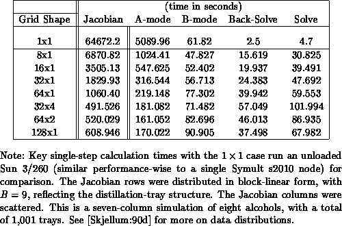
Table 9.6:
Order 9009 Dynamic Simulation Data
If we utilize latency
in the Jacobian calculation, we
could reduce the sequential time by a factor of about 100. This
improvement would also carry through to the concurrent times for
Jacobian solution. At that ratio, Jacobian computation to B-mode
factorization has a sequential ratio of about 10:1. As is, we achieve
legitimate speedups of about five. We expect to improve these results
using the ideas quoted elsewhere in this book and in
[
Skjellum:90d
].
From a modelling point-of-view, two things are important to note.
First, the introduction of more nonideal thermodynamics would improve
speedup, because these calculations fall within the Jacobian
computation phase and single-residual computation. Furthermore, the
introduction of a more realistic model will likewise bear on
concurrency, and likely improve it. For example, introducing flow
dynamics, enthalpy balances, and vapor holdups makes the model more
difficult to solve numerically (higher index). It also increases the
chance for a wide range of stepsizes, and the possible need for
additional A-mode factorizations to maintain stability in the
integration process. Such operations are more costly, but also have a
higher speedup. Furthermore, the more complex models will be less
likely to have near diagonal dominance; consequently more
pivoting
is to be expected, again increasing the
chance for overall speedup compared to the sequential case. Mainly, we
plan to consider the waveform-relaxation
approach more heavily, and also to consider new classes of dynamic
distillation simulations with Concurrent DASSL [
Skjellum:90c
].
Next:
9.6.6 Conclusions
Up:
Concurrent DASSL Applied
Previous:
Residual Communication
Guy Robinson
Wed Mar 1 10:19:35 EST 1995
9.6.6 Conclusions
Next:
9.7 Adaptive Multigrid
Up:
Concurrent DASSL Applied
Previous:
9.6.5 Chemical Engineering Example
We have developed a high-quality concurrent code, Concurrent DASSL, for
the solution of ordinary differential-algebraic equations
of low index. This code, together with
appropriate linear algebra and simulation layers, allows us to explore
the achievable concurrent performance of nontrivial problems. In
chemical engineering,
we have applied it
thus far to a reasonably large, simple model of coupled distillation
columns. We are able to solve this large problem, which is quite
demanding on even a large mainframe because of huge memory requirements
and nontrivial computational requirements; the speedups achieved thus
far are legitimately at least five, when compared to an efficient
sequential implementation. This illustrates the need for improvements
to the linear algebra code, which are feasible because sparse matrices
will admit multiple pivots heuristically. It also illustrates the need
to consider hidden sources of additional timelike concurrency in
Concurrent DASSL, perhaps allowing multiple right-hand sides to be
attacked simultaneously by the linear algebra codes, and amortizing
their cost more efficiently. Furthermore, the performance points up
the need for detailed research into novel numerical techniques, such as
waveform relaxation, which we have begun to do as well
[
Skjellum:88a
].
Guy Robinson
Wed Mar 1 10:19:35 EST 1995
9.7 Adaptive Multigrid
Next:
9.7.1 Introduction
Up:
9 Loosely Synchronous Problems
Previous:
9.6.6 Conclusions
Guy Robinson
Wed Mar 1 10:19:35 EST 1995
9.7.1 Introduction
Next:
9.7.2 The Basic Algorithm
Up:
9.7 Adaptive Multigrid
Previous:
9.7 Adaptive Multigrid
Simple relaxation methods reduce the high-frequency components of the
solution error by an order of magnitude in a few iterations. This
observation is used to derive the multigrid
method; see Brandt [
Brandt:77a
], Hackbusch [
Hackbusch:85a
];
Hackbusch and Trottenberg [
Hackbusch:82a
]. In the multigrid
method,
a smoothed problem is projected to a
coarser grid. This coarse-grid problem is then solved recursively by
smoothing and coarse-grid correction. The recursion terminates on the
coarsest grid, where an exact solver is used. In the full multigrid
method, a coarser grid is also used to compute an initial guess for the
multigrid iteration on a finer grid. With this method, it is possible
to solve the problem with an operation count proportional to the number
of unknowns.
Multigrid methods are best understood for elliptic problems, that is,
the Poisson equation, stationary reaction-diffusion equations, implicit
time-steps in parabolic problems, and so on. However, the multigrid
approach is also successful for many other applications, from fluid
flow to computer vision. Parallelization issues are independent of
particular applications, and elliptic problems are a good test bed for
the study of concurrent multigrid. We chose two- and three-dimensional
stationary nonlinear reaction-diffusion equations in a rectangular
domain  as our model problem, that is,

with suitable boundary conditions.
To parallelize multigrid, we proceed as follows (see also [
Velde:87a
],
[
Velde:87b
]). First, a sequential multigrid procedure is developed.
Here, the basic numerical problems are addressed: which smoothing,
restriction, and prolongation operators to use, the resolution required (size
of the finest grid), the number of levels (size of the coarsest grid), and
the coarsest-grid solver. Second, this sequential multigrid code is
generalized to include local grid refinement (in the neighborhood of
singularities, for example). Three basic problems are addressed in this
second stage: the algorithmic aspect of local grid refinement, the numerical
treatment of interior boundaries, and the relaxation of partially overlapping
grid patches. In the third and last step, the multigrid code is
parallelized. This can now be done without introducing new numerical issues.
Each concurrent process starts a sequential multigrid procedure, each one
locally refining to a particular subdomain. To achieve this, a communication
operation for the exchange of interior boundary values is needed. Depending
on the size of the coarsest grid, it might be required to develop,
independently, a concurrent coarsest grid solver.
This parallelization strategy has the advantage that all numerical problems
can be addressed in the sequential stages. Although our implementation is
for regular grids, the same strategy is also valid for irregular grids.
Next:
9.7.2 The Basic Algorithm
Up:
9.7 Adaptive Multigrid
Previous:
9.7 Adaptive Multigrid
Guy Robinson
Wed Mar 1 10:19:35 EST 1995
9.7.2 The Basic Algorithm
Next:
9.7.3 The Adaptive Algorithm
Up:
9.7 Adaptive Multigrid
Previous:
9.7.1 Introduction
To simplify the switch to adaptive grids later, we use a multigrid
variant known as the
full approximation scheme
. Thus, on every
level, we compute an approximation to the solution of the original
equation, not of an error equation. This multigrid procedure is
defined by the following basic building blocks: a coarsest-grid
solver, a solution restriction operator, a right-hand-side restriction
operator, a prolongation operator, and a smoothing operator.
Two feasible coarsest-grid solvers are relaxation until
convergence
and a direct solver (embedded in a
Newton iteration if the problem is nonlinear). The cost of solving a
problem on the coarsest grid is, of course, related to the size of the
coarsest grid. If the coarsest grid is very coarse, the cost is
negligible. However, numerical reasons often dictate a minimum
resolution for the coarsest grid. Moreover, elaborate computations may
take place on the coarsest grid; see [
Bolstadt:86a
],
[
Chan:82a
], [
Dinar:85a
] for examples of multigrid
continuation. In some instances, the performance of the computations
on the coarsest grids cannot be neglected.
Many alternatives exist for smoothing. Parallelization will be easiest with
point relaxations. Jacobi underrelaxation and red-black Gauss-Seidel
relaxation are particularly suited for concurrent implementations and for
adaptive grids. Hence, we shall restrict our attention to point relaxation
methods.
The intergrid transfers are usually simple: linear interpolation as the
prolongation operator, injection or full-weight restriction as the
restriction operator.
The main data structure of the sequential nonadaptive algorithm is a doubly
linked list
of grids, where a grid structure
provides memory for the solution and right-hand-side vectors, and each
grid is connected to one finer and one coarser grid. The sequential
multigrid code has the following structure: a library of operations
on grid functions, a code related to the construction of a doubly
linked list of grids, and the main multigrid algorithm. We maintain
this basic structure for the concurrent and adaptive algorithms.
Although the doubly linked list of grids will be replaced by a more
complex structure, the basic multigrid algorithm will not be altered.
While the library of grid function operations will be expanded, the
fundamental operations will remain the same. This is important,
because the basic library for a general multigrid package with several
options for each operator is large.
Next:
9.7.3 The Adaptive Algorithm
Up:
9.7 Adaptive Multigrid
Previous:
9.7.1 Introduction
Guy Robinson
Wed Mar 1 10:19:35 EST 1995
9.7.3 The Adaptive Algorithm
Next:
9.7.4 The Concurrent Algorithm
Up:
9.7 Adaptive Multigrid
Previous:
9.7.2 The Basic Algorithm
Here, we focus on the use of adaptive grids for sequential computations. We
shall apply these ideas in the next section to achieve concurrency.
Figure
9.16
illustrates the grid structure of a one-dimensional
adaptive multigrid procedure. Fine grids are introduced only where
necessary, in the neighborhood of a singularity, for example. In two and
three dimensions the topology is more complicated, and it makes sense to
refine in several subdomains that partially overlap.
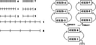
Figure 9.16:
One-Dimensional Adaptive Multigrid Structure
We focus first on the intergrid transfers. Although these operators are
straightforward, they are the source of some implementation difficulties for
the concurrent algorithm, because load-balanced data distributions of fine and
coarse grids are not compatible. The structure introduced here avoids these
difficulties. Before introducing a fine grid on a subdomain, we construct
an artificial coarse grid on the same subdomain. This artificial coarse
grid, called a
child grid
, differs from a normal grid data structure only
because its data vectors (the solution and right-hand side) are subvectors of
the parent-grid data vectors. Thus, child grids do not use extra memory for
data (except for some negligible amount for bookkeeping). In
Figure
9.16
, grid 1 is a parent-grid with two children, grids 2
and 3. With child grids, the intergrid transfers of the nonadaptive
procedure can be reused. The restriction, for example, takes place between a
fine grid (defined over a subdomain) and a coarse child grid (in
Figure
9.16
, between grids 4 and 2 and between grids 5 and 3,
respectively). Because data memory of child and parent grid are shared, the
appropriate subvectors of the coarse grid data are updated automatically.
Similarly, prolongation occurs between the child grid and the fine grid.
The basic data structure of the nonadaptive procedure, the doubly linked list
of grids, is transformed radically as a result of child grids and their
refinements. The data structure is now a tree of doubly linked
lists;
see Figure
9.16
. As mentioned
before, the intergrid transfers are not affected by this complicated
structure. For relaxation, the only significant difference is that
more than one grid may have to be relaxed on each level. When the
boundary of one grid intersects the interior of another grid on the
same level, the boundary values must be interpolated
(Figure
9.17
). This does not affect the relaxation
operators, as long as the relaxation step is preceded by a
boundary-interpolation step.

Figure 9.17:
Boundary Interpolation
Next:
9.7.4 The Concurrent Algorithm
Up:
9.7 Adaptive Multigrid
Previous:
9.7.2 The Basic Algorithm
Guy Robinson
Wed Mar 1 10:19:35 EST 1995
9.7.4 The Concurrent Algorithm
Next:
9.7.5 Summary
Up:
9.7 Adaptive Multigrid
Previous:
9.7.3 The Adaptive Algorithm
The same structure that made the multigrid code adaptive allows us to
parallelize it. For now, assume that every process starts out with a copy of
the coarsest grid, defined on the whole domain. Each process is assigned a
subdomain in which to compute the solution to maximum accuracy. The collection
of subdomains assigned to all processes covers the computational domain.
Within each process, an adaptive grid structure is constructed so that the
finest level at which the solution is needed envelops the assigned subdomain;
see Figure
9.18
. The set of all grids (in whatever process they
reside) forms a tree structure like the one described in the previous section.
The same algorithm can be applied to it. Only one addition must be made to
the program: overlapping grids on the same level but residing in different
processes must communicate in order to interpolate boundary values. This is
an operation to be added to the basic library.
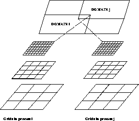
Figure 9.18:
Use of Adaptive Multigrid for Concurrency
The coarsest grid can often be ignored as far as machine efficiency is
concerned. As mentioned in Section
9.7.2
, the computations on the
coarsest grid are sometimes substantial. In such cases, it is crucial
to parallelize the coarsest-grid computations. With relaxation until
convergence
as the coarsest-grid solver, one could
simply divide up the coarsest grid over all concurrent processes. It
is more likely, however, that the coarsest-grid computations involve a
direct solution method. In this case, the duplicated coarsest grid is
well suited as an interface to a concurrent direct solver, because it
simplifies the initialization of the coefficient matrix. We refer to
Section
8.1
and [
Velde:90a
] for details on some direct
solvers.
The total algorithm, adaptive multigrid and concurrent coarsest grid
solver, is heterogeneous: its communication structure is irregular and
varies significantly from one part of the program to the next, making
the data distribution for optimal load balance
difficult to predict. On the coarsest level, we achieve load balance
by exploiting the data distribution independence of our linear algebra
code; see [
Lorenz:92a
]. On the finer levels, load balance is
obtained by allocating an approximately equal number of finest-grid
points to each process.
Next:
9.7.5 Summary
Up:
9.7 Adaptive Multigrid
Previous:
9.7.3 The Adaptive Algorithm
Guy Robinson
Wed Mar 1 10:19:35 EST 1995
9.7.5 Summary
Next:
9.8 Munkres Algorithm for
Up:
9.7 Adaptive Multigrid
Previous:
9.7.4 The Concurrent Algorithm
The concurrent multigrid program was developed by Eric F. Van de Velde.
Associated C P references are [
Lorenz:89a
], [
Lorenz:92a
],
[
Velde:87a
], [
Velde:87b
], [
Velde:89b
], [
Velde:90a
].
P references are [
Lorenz:89a
], [
Lorenz:92a
],
[
Velde:87a
], [
Velde:87b
], [
Velde:89b
], [
Velde:90a
].
Guy Robinson
Wed Mar 1 10:19:35 EST 1995
9.8 Munkres Algorithm for Assignment
Next:
9.8.1 Introduction
Up:
9 Loosely Synchronous Problems
Previous:
9.7.5 Summary
Guy Robinson
Wed Mar 1 10:19:35 EST 1995
9.8.1 Introduction
Next:
9.8.2 The Sequential Algorithm
Up:
9.8 Munkres Algorithm for
Previous:
9.8 Munkres Algorithm for
The so-called
assignment problem
is of
considerable importance in a variety of applications, and can be stated as
follows. Let

and

be two sets of items, and let

be a measure of the distance (dissimilarity) between individual items from
the two lists. Taking  , the objective of the assignment
problem is to find the particular mapping
, the objective of the assignment
problem is to find the particular mapping


such that the total association score

is minimized over all permutations  .
.
For  , the naive (exhaustive search) complexity of the
assignment problem is
, the naive (exhaustive search) complexity of the
assignment problem is  . There are,
however, a variety of exact solutions to the assignment problem with reduced
complexity
. There are,
however, a variety of exact solutions to the assignment problem with reduced
complexity  ([
Blackman:86a
], [
Burgeios:71a
],
[
Kuhn:55a
]). Section
9.8.2
briefly describes one such method,
Munkres algorithm
[
Kuhn:55a
], and presents a
particular sequential
implementation. Performance of the algorithm is examined for the
particularly nasty problem of associating lists of random points within the
unit square. In Section
9.8.3
, the algorithm is generalized for
concurrent execution, and performance results for runs on the Mark III
hypercube are presented.
([
Blackman:86a
], [
Burgeios:71a
],
[
Kuhn:55a
]). Section
9.8.2
briefly describes one such method,
Munkres algorithm
[
Kuhn:55a
], and presents a
particular sequential
implementation. Performance of the algorithm is examined for the
particularly nasty problem of associating lists of random points within the
unit square. In Section
9.8.3
, the algorithm is generalized for
concurrent execution, and performance results for runs on the Mark III
hypercube are presented.
Guy Robinson
Wed Mar 1 10:19:35 EST 1995
9.8.2 The Sequential Algorithm
Next:
9.8.3 The Concurrent Algorithm
Up:
9.8 Munkres Algorithm for
Previous:
9.8.1 Introduction
The input to the assignment problem is the matrix  of dissimilarities from Equation
9.19
. The first point to note
is that the particular assignment which minimizes Equation
9.21
is not altered if a
fixed
value is added to or subtracted from all
entries in any row or column of the cost matrix
D
. Exploiting this fact,
Munkres' solution to the assignment problem can be divided into two parts
of dissimilarities from Equation
9.19
. The first point to note
is that the particular assignment which minimizes Equation
9.21
is not altered if a
fixed
value is added to or subtracted from all
entries in any row or column of the cost matrix
D
. Exploiting this fact,
Munkres' solution to the assignment problem can be divided into two parts
-
M1:
-
Modifications of the distance matrix
D
by row/column
subtractions, creating a (large) number of zero entries.
-
M2:
-
With
 denoting the row indices of all zeros in
column
i
, construction of a so-called
minimal representative set
,
meaning a distinct selection
denoting the row indices of all zeros in
column
i
, construction of a so-called
minimal representative set
,
meaning a distinct selection  for each
i
, such that
for each
i
, such that
 .
.
The steps of Munkres algorithm generally follow those in the constructive
proof of P. Hall's theorem on minimal representative sets.
The preceding paragraph provides a hopelessly incomplete hint as to the
number theoretic basis for Munkres algorithm. The particular implementation
of Munkres algorithm used in this work is as described in Chapter 14 of
[
Blackman:86a
]. To be definite, take  and let the
columns of the distance matrix be associated with items from list
and let the
columns of the distance matrix be associated with items from list  .
The first step is to subtract the smallest item in each column from all
entries in the column. The rest of the algorithm can be viewed as a search
for
special
zero entries (starred zeros
.
The first step is to subtract the smallest item in each column from all
entries in the column. The rest of the algorithm can be viewed as a search
for
special
zero entries (starred zeros  ), and proceeds as
follows:
), and proceeds as
follows:
Munkres Algorithm
-
Step 1:
-
Setup
-
Find a zero
Z
in the distance matrix.
-
If there is no starred zero already in its row or column, star this
zero.
-
Repeat steps 1.1, 1.2 until all zeros have been considered.
-
Step 2:
-
 Count, Solution Assessment
-
Cover every column containing a
 .
.
-
Terminate the algorithm if all columns are covered. In this case, the
locations of the
 entries in the matrix provide the solution to
the assignment problem.
entries in the matrix provide the solution to
the assignment problem.
-
Step 3:
-
Main Zero Search
-
Find an uncovered
Z
in the distance matrix and prime it,
 . If no such zero exists, go to Step 5
-
If No
 exists in the row of the
  , go to Step 4.
-
If a
 exists, cover this row and uncover the column of
the
exists, cover this row and uncover the column of
the  . Return to Step 3.1 to find a new
Z
.
. Return to Step 3.1 to find a new
Z
.
-
Step 4:
-
Increment Set of Starred Zeros
-
Construct the ``alternating sequence'' of primed and starred zeros:
-
-
 : Unpaired
  from Step 3.2
-
-
 : The
: The  in the column of
-
-
 : The
: The  in the row of
  ,
if
such a zero exists
,
if
such a zero exists
-
-
 : The
: The  in the column of
The sequence eventually terminates with an unpaired  for some
N
.
for some
N
.
-
Unstar each starred zero of the sequence.
-
Star each primed zero of the sequence, thus increasing the number of
starred zeros by one.
-
Erase all primes, uncover all columns and rows, and return to Step 2.
-
Step 5:
-
New Zero Manufactures
-
Let
h
be the smallest uncovered entry in the (modified) distance
matrix.
-
Add
h
to all covered rows.
-
Subtract
h
from all uncovered columns
-
Return to Step 3, without altering stars, primes, or covers.
A (very) schematic flowchart for the algorithm is shown in
Figure
9.19
. Note that Steps 1,5 of the algorithm overwrite
the original distance matrix.
The preceding algorithm involves flags (starred or primed) associated with
zero entries in the distance matrix, as well as ``covered'' tags associated
with individual rows and columns. The implementation of the zero tagging is
done by first noting that there is
at most
one  or
or  in any row or column. The covers and zero tags of the algorithm are
accordingly implemented using five simple arrays:
in any row or column. The covers and zero tags of the algorithm are
accordingly implemented using five simple arrays:
-
CC
 :
:
-
Covered column tags,
 .
.
-
CR
 :
:
-
Covered row tags,

-
ZS
 :
:
-
 locators for columns of the matrix. If positive,
ZS
locators for columns of the matrix. If positive,
ZS is the row index of the
  in the
  column of the matrix.
-
ZR
 :
:
-
 locators for rows of the matrix. If positive,
ZR
locators for rows of the matrix. If positive,
ZR is the column of the
  in the
  row of the matrix.
-
ZP
 :
:
-
 locators for rows of the matrix. If positive,
ZP
locators for rows of the matrix. If positive,
ZP is the column of the
  in the
  row of the matrix.
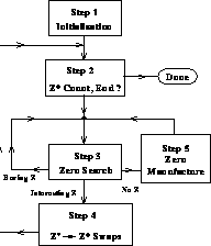
Figure 9.19:
Flowchart for Munkres Algorithm
Entries in the cover arrays CC and CR are one if the row or column is covered
zero otherwise. Entries in the zero-locator arrays ZS, ZR, and ZP are zero if
no zero of the appropriate type exists in the indexed row or column.
With the star-prime-cover scheme of the preceding paragraph, a sequential
implementation of Munkres algorithm is completely straightforward. At the
beginning of Step 1, all cover and locator flags are set to zero, and the
initial zero search provides an initial set of nonzero entries in ZS().
Step 2 sets appropriate entries in CC() to one and simply counts the covered
columns. Steps 3 and 5 are trivially implemented in terms of the
cover/zero arrays and the ``alternating sequence'' for Step 4 is readily
constructed from the contents of ZS(), ZR() and ZP().
As an initial exploration of Munkres algorithm, consider the task of
associating two lists of random points within a 2D unit square, assuming
the cost function in Equation
9.19
is the usual
Cartesian
distance. Figure
9.20
plots
total CPU times for execution of Munkres algorithm for equal size lists
versus list size. The vertical axis gives CPU times in seconds for one
node of the Mark III hypercube. The circles and crosses show the time
spent in Steps 5 and 3, respectively. These two steps (zero search
and zero manufacture) account for essentially
all
of the CPU
time. For the  case, the total CPU time spent in Step 2
was about
case, the total CPU time spent in Step 2
was about  , and that spent in Step 4 was too small
to be reliably measured. The large amounts of time spent in Steps 3 and
5 arise from the very large numbers of times these parts of the
algorithm are executed. The
, and that spent in Step 4 was too small
to be reliably measured. The large amounts of time spent in Steps 3 and
5 arise from the very large numbers of times these parts of the
algorithm are executed. The  case involves 6109 entries
into Step 3 and 593 entries into Step 5.
case involves 6109 entries
into Step 3 and 593 entries into Step 5.
Since the zero searching in Step 3 of the algorithm is required so often, the
implementation of this step is done with some care. The search for zeros is
done column-by-column, and the code maintains pointers to both the last
column searched and the most recently uncovered column (Step 3.3) in order to
reduce the time spent on subsequent re-entries to the Step 3 box of
Figure
9.19
.
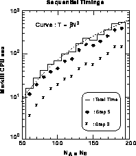
Figure 9.20:
Timing Results for the Sequential Algorithm Versus Problem Size
The dashed line of Figure
9.20
indicates the nominal
 scaling predicted for Munkres algorithm. By and
large, the timing results in Figure
9.20
are consistent with
this expected behavior. It should be noted, however, that both the nature of
this scaling and the coefficient of
scaling predicted for Munkres algorithm. By and
large, the timing results in Figure
9.20
are consistent with
this expected behavior. It should be noted, however, that both the nature of
this scaling and the coefficient of  are very dependent on the nature
of the data sets. Consider, for example, two identical trivial lists
are very dependent on the nature
of the data sets. Consider, for example, two identical trivial lists

with the distance between items given by the absolute value function. For the
data sets in Equation
9.22
, the preliminaries and Step 1 of
Munkres algorithm completely solve the association in a time which scales as
 . In contrast, the random-point association problem is a much greater
challenge for the algorithm, as nominal pairings indicated by the initial
nearest-neighbor searches of the preliminary step are tediously undone in the
creation of the staircaselike sequence of zeros needed for Step 4. As a
brief, instructive illustration of the nature of this processing,
Figure
9.21
plots the CPU time
per step
for the last
passes through the outer loop of Figure
9.19
for the
150
. In contrast, the random-point association problem is a much greater
challenge for the algorithm, as nominal pairings indicated by the initial
nearest-neighbor searches of the preliminary step are tediously undone in the
creation of the staircaselike sequence of zeros needed for Step 4. As a
brief, instructive illustration of the nature of this processing,
Figure
9.21
plots the CPU time
per step
for the last
passes through the outer loop of Figure
9.19
for the
150 150 assignment problem (recall that each pass through the outer
loop increases the
150 assignment problem (recall that each pass through the outer
loop increases the  count by one). The processing load per step is
seen to be highly nonuniform.
count by one). The processing load per step is
seen to be highly nonuniform.
Figure 9.21:
Times Per Loop (i.e.,  increment) for the Last Several
Loops in the Solution of the
increment) for the Last Several
Loops in the Solution of the  Problem
Next:
9.8.3 The Concurrent Algorithm
Up:
9.8 Munkres Algorithm for
Previous:
9.8.1 Introduction
Guy Robinson
Wed Mar 1 10:19:35 EST 1995
9.8.3 The Concurrent Algorithm
Next:
Optimization Methods
for
Up:
9.8 Munkres Algorithm for
Previous:
9.8.2 The Sequential Algorithm
The timing results from Figure
9.20
clearly dictate the manner
in which the calculations in Munkres algorithm should be distributed among
the nodes of a hypercube for concurrent execution. The zero and minimum
element searches for Steps 3 and 5 are the most time consuming and should
be done concurrently. In contrast, the essentially bookkeeping tasks
associated with Steps 2 and 4 require insignificant CPU time and are most
naturally done in lockstep (i.e., all nodes of the hypercube perform the same
calculations on the same data at the same time). The details of the
concurrent algorithm are as follows.
Data Decomposition
The distance matrix  is distributed across the
nodes of the hypercube, with entire columns assigned to individual
nodes. (This assumes, effectively, that
is distributed across the
nodes of the hypercube, with entire columns assigned to individual
nodes. (This assumes, effectively, that  ,
which is always the case for assignment problems which are big enough
to be ``interesting.'') The cover and zero locator lists defined in
Section
9.8.2
are duplicated on all nodes.
,
which is always the case for assignment problems which are big enough
to be ``interesting.'') The cover and zero locator lists defined in
Section
9.8.2
are duplicated on all nodes.
Task Decomposition
The concurrent implementation of Step 5 is particularly
trivial. Each node first finds its own minimum uncovered value,
setting this value to some ``infinite'' token if all columns assigned
to the node are covered. A simple loop on communication channels
determines the global minimum among the node-by-node minimum values,
and each node then modifies the contents of its local portion of the
distance matrix according to Steps 5.2 and 5.3.
The concurrent implementation of Step 3 is just slightly more awkward. On
entry to Step 3, each node searches for zeros according to the rules of
Section
9.8.2
, and fills a three-element status list:

where
S
is a zero-search status flag,

If the status is nonnegative, the last two entries in the status list
specify the location of the found zero. A simple channel loop is used to
collect the individual status lists of each node into all nodes, and the
action taken next by the program is as follows:
-
If all nodes give negative status (no
Z
found), all nodes proceed
to Step 5.
-
If any node gives status one, all nodes proceed to Step 4 for lockstep
updates of the zero location lists, using the row-column indices of the node
which gave status one as the starting point for Step 4.1. If more than one
node returns status one (highly unlikely, in practice), only the first such
node (lower node number) is used.
-
If all zeros uncovered are ``Boring,'' the cover switching in Step 3.3
of the algorithm is performed. This is done in lockstep, processing the
Z
s
returned by the nodes in order of increasing node number. Note that the cover
rearrangements performed for one node may well cover a
Z
returned by a node
with a higher node number. In such cases, the nominal
Z
returned by the
later node is simply ignored.
It is worth emphasizing that only the actual
searches
for zero and
minimum entries in Steps 3 and 5 are done concurrently. The updates of
the cover and zero locator lists are done in unison.
The concurrent algorithm has been implemented on the Mark III hypercube, and
has been tested against random point association tasks for a variety of list
sizes. Before examining results of these tests, however, it is worth noting
that the concurrent implementation is not particularly dependent on the
hypercube topology. The only communication-dependent parts of the algorithm
are
-
Determination of the ensemble-wide minimum value for Step 5;
-
Collection of the local Step 3 status lists
(Equation
9.24
),
either of which could be easily done for almost any MIMD architecture.
Table
9.7
presents performance results for the association of
random lists of 200 points on the Mark III hypercube for various cube
dimensions. (For consistency, of course, the same input lists are used for
all runs.) Time values are given in CPU seconds for the total execution
time, as well as the time spent in Steps 3 and 5. Also given are the
standard concurrent execution efficiencies,

as well as the number of times the Step 3 box of Figure
9.19
is entered during execution of the algorithm. The numbers of entries into
the other boxes of Figure
9.19
are independent of the hypercube
dimension.
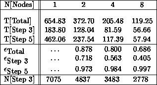
Table 9.7:
Concurrent Performance for  Random Points. T
is time,
Random Points. T
is time,  efficiency, and N[Step 3] the number of times
Step 3 is executed.
efficiency, and N[Step 3] the number of times
Step 3 is executed.
There is an aspect of the timing results in Table
9.7
which
should be noted. Namely, essentially
all
inefficiencies of the
concurrent algorithm are associated with Step 3 for two nodes compared to
Step 3 for one node. The times spent in Step 5 are approximately halved for
each increase in the dimension of the hypercube. However, the efficiencies
associated with the zero searching in Step 3 are rather poorer, particularly
for larger numbers of nodes.
At a simple, qualitative level, the inefficiencies associated with Step 3 are
readily understood. Consider the task of finding a single zero located
somewhere inside an  matrix. The mean sequential search time is

since, on average, half of the entries of the matrix will be examined before
the zero is found. Now consider the same zero search on two nodes. The node
which has the half of the matrix containing the zero will find it in about
half the time of Equation
9.26
.
However
, the other node
will
always
search through all of its  items before
returning a null status for Equation
9.24
. Since the node
which found the zero must wait for the other node before the (lockstep)
modifications of zero locators and cover tags, the node without the zero
determines the actual time spent in Step 3, so that
items before
returning a null status for Equation
9.24
. Since the node
which found the zero must wait for the other node before the (lockstep)
modifications of zero locators and cover tags, the node without the zero
determines the actual time spent in Step 3, so that

In the full program, the concurrent bottleneck is not as bad as
Equation
9.27
would imply. As noted above, the concurrent
algorithm can process multiple ``Boring'' Zs in a single pass through Step 3.
The frequency of such multiple Zs per step can be estimated by noting the
decreasing number of times Step 3 is entered with increasing hypercube
dimension, as indicated in Table
9.7
. Moreover, each node
maintains a counter of the last column searched during Step 3. On subsequent
re-entries, columns prior to this marked column are searched for zeros only
if they have had their cover tag changed during the prior Step 3 processing.
While each of these algorithm elements does diminish the problems associated
with Equation
9.27
, the fact remains that the search for zero
entries in the distributed distance matrix is the least efficient step in
concurrent implementations of Munkres algorithm.
The results presented in Table
9.7
demonstrate that an
efficient implementation of Munkres algorithm is certainly feasible.
Next, we examine how these efficiencies change as the problem size
is varied.
The results shown in Tables
9.8
and
9.9
demonstrate an improvement of concurrent efficiencies with increasing problem
size-the expected result. For the  problem on eight nodes,
the efficiency is only about 50%. This problem is too small for eight
nodes, with only 12 or 13 columns of the distance matrix assigned to
individual nodes.
problem on eight nodes,
the efficiency is only about 50%. This problem is too small for eight
nodes, with only 12 or 13 columns of the distance matrix assigned to
individual nodes.
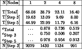
Table 9.8:
Concurrent Performance for  Random Points
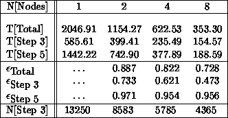
Table 9.9:
Concurrent Performance for  Random Points
While the performance results in Tables
9.7
through
9.9
are certainly acceptable, it is nonetheless
interesting to investigate possible improvements of efficiency for the
zero searches in Step 3. The obvious candidate for an algorithm
modification is some sort of checkpointing: At intermediate times
during the zero search, the nodes exchange a ``Zero Found Yet?'' status
flag, with all nodes breaking out of the zero search loop if any node
returns a positive result.
For message-passing machines such as the Mark III, the checkpointing scheme is
of little value, as the time spent in individual entries to Step 3 is not
enormous compared to the node-to-node communication time. For example, for
the two-node solution of the  problem, the mean time for a
single entry to Step 3 is only about
problem, the mean time for a
single entry to Step 3 is only about  , compared to a typical
node-to-node communications time which can be a significant fraction of a
millisecond. The time required to perform a single Step 3 calculation is not
large compared to node-to-node communications. As a (not unexpected)
consequence, all attempts to improve the Step 3 efficiencies through various
``Found Anything?'' schemes were completely unsuccessful.
, compared to a typical
node-to-node communications time which can be a significant fraction of a
millisecond. The time required to perform a single Step 3 calculation is not
large compared to node-to-node communications. As a (not unexpected)
consequence, all attempts to improve the Step 3 efficiencies through various
``Found Anything?'' schemes were completely unsuccessful.
The checkpointing difficulties for a message-passing machine could disappear,
of course, on a shared-memory machine. If the zero-search status flags for
the various nodes could be kept in memory locations readily (i.e., rapidly)
accessible to all nodes, the problems of the preceding paragraph might be
eliminated. It would be interesting to determine whether significant
improvements on the (already good) efficiencies of the concurrent Munkres
algorithm could be achieved on a shared-memory machine.
Next:
Optimization Methods
for
Up:
9.8 Munkres Algorithm for
Previous:
9.8.2 The Sequential Algorithm
Guy Robinson
Wed Mar 1 10:19:35 EST 1995
Optimization Methods
for Neural Nets:Automatic Parameter Tuning and
FasterConvergence
Next:
9.9.1 Deficiencies of Steepest
Up:
9 Loosely Synchronous Problems
Previous:
9.8.3 The Concurrent Algorithm
Computers and standard programming languages can be used efficiently
for high-level, clearly formulated problems such as computing balance
sheets and income statements, solving partial differential equations,
or managing operations in a car factory. It is much more difficult to
write efficient and fault-tolerant programs for ``simple'' primitive
tasks like hearing, seeing, touching, manipulating parts, recognizing
faces, avoiding obstacles, and so on. Usually, the existing artificial
systems for the above tasks are within a narrowly limited domain of
application, very sensitive to hardware and software failures, and
difficult to modify and adapt to new environments.
Neural nets
represent a new approach to bridging the gap
between cheap computational power and solutions for some of the above-cited
tasks. We as human beings like to consider ourselves good examples of the
power of the neuronal approach to problem solving.
To avoid naive optimism and over inflated expectations about
``self-programming'' computers, it is safer to see this development as
the creation of another level of tools insulating generic users looking
for fast solutions from the details of sophisticated learning
mechanisms. Today, generic users do not care about writing operating
systems; in the near future
some
users will not care about
programming and debugging.
They will have to choose
appropriate off-the-shelf subsystems (both hardware and software) and
an appropriate set of examples and high-level specifications; neural
nets
will do the rest. Neural networks have
already been useful in areas like pattern classification,
robotics,
system modeling, and forecasting over time
([
Borsellino:61a
], [
Broomhead:88a
], [
Gorman:88a
],
[
Sejnowski:87a
], [
Rumelhart:86b
], [
Lapedes:87a
]).
The focus of this work is on ``supervised learning'', that is, learning
an association between input and output patterns from a set of
examples. The mapping is executed by a feed-forward network with
different layers of units, such as the one shown in
Figure
9.22
.
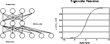
Figure 9.22:
Multilayer Perceptron and Transfer Function
Each unit that is not in the input layer receives an input given by a
weighted sum of the outputs of the previous layer and produces an output
using a ``sigmoidal'' transfer function, with a linear range and saturation
for large positive and negative inputs. This particular architecture has
been considered because it has been used extensively in neural network
research, but the learning method presented can be used for different network
designs ([
Broomhead:88a
]).
Next:
9.9.1 Deficiencies of Steepest
Up:
9 Loosely Synchronous Problems
Previous:
9.8.3 The Concurrent Algorithm
Guy Robinson
Wed Mar 1 10:19:35 EST 1995
9.9.1 Deficiencies of Steepest Descent
Next:
9.9.2 The ``Bold Driver''
Up:
Optimization Methods
for
Previous:
Optimization Methods
for
The multilayer perceptron, initialized with random weights, presents random
output patterns. We would like to execute a learning stage, progressively
modifying the values of the connection strengths in order to make the outputs
nearer to the prescribed ones.
It is straightforward to transform the learning task into an
optimization
problem (i.e., a search for the minimum of a specified function,
henceforth called
energy
). If the
energy
is defined as the sum
of the squared errors between
obtained
and
desired
output
pattern over the set of examples, minimizing it will accomplish the task.
A large fraction of the theoretical and applied research in supervised
learning is based on the
steepest descent
method for minimization.
The negative gradient of the energy with respect to the weights is
calculated during each iteration, and a step is taken in that direction (if
the step is small enough, energy reduction is assured). In this way, one
obtains a sequence of weight vectors,  , that converges to a
local minimum of the energy function:
, that converges to a
local minimum of the energy function:

Now, given that we are interested in converging to the local minimum in the
shortest time (this is not always the case: to combat noise some slowness may
be desired), there is no good reason to restrict ourselves to steepest
descent, and there are at least a couple of reasons in favor of other
methods. First, the
learning speed
,  , is a free
parameter that has to be chosen carefully for each problem (if it is too
small, progress is slow; if too large, oscillations may be created).
Second, even in the optimal case of a step along the steepest descent
direction bringing the system to the absolute minimum (
along this
direction
), it can be proved that steepest descent can be arbitrarily slow,
particularly when ``the search space contains long ravines that are
characterized by sharp curvature across the ravine and a gently sloping
floor'' [
Rumelhart:86b
]. In other words, if we are unlucky with the
choice of units along the different dimensions (and this is a frequent event
when the number of weights is 1000 or 10,000), it may be the case that during
each iteration, the previous error is reduced by 0.000000001%!
, is a free
parameter that has to be chosen carefully for each problem (if it is too
small, progress is slow; if too large, oscillations may be created).
Second, even in the optimal case of a step along the steepest descent
direction bringing the system to the absolute minimum (
along this
direction
), it can be proved that steepest descent can be arbitrarily slow,
particularly when ``the search space contains long ravines that are
characterized by sharp curvature across the ravine and a gently sloping
floor'' [
Rumelhart:86b
]. In other words, if we are unlucky with the
choice of units along the different dimensions (and this is a frequent event
when the number of weights is 1000 or 10,000), it may be the case that during
each iteration, the previous error is reduced by 0.000000001%!
The problem is essentially caused by the fact that the gradient does not
necessarily point in the direction of the minimum, as it is shown in
Figure
9.23
.
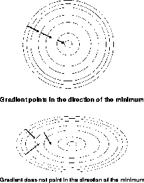
Figure 9.23:
Gradient Direction for Different Choice of Units
If the energy is quadratic, a large ratio of the maximum to minimum
eigenvalues
causes the ``zigzagging'' motion
illustrated. In the next sections, we will illustrate two suggestions
for tuning parameters in an adaptive way and selecting better descent
directions.
Next:
9.9.2 The ``Bold Driver''
Up:
Optimization Methods
for
Previous:
Optimization Methods
for
Guy Robinson
Wed Mar 1 10:19:35 EST 1995
9.9.2 The ``Bold Driver'' Network
Next:
The Broyden-Fletcher-Goldfarb-Shanno
One-StepMemoryless
Up:
Optimization Methods
for
Previous:
9.9.1 Deficiencies of Steepest
There are
no general prescriptions
for selecting an appropriate
learning
rate  in back-propagation, in order
to avoid oscillations and converge to a good local minimum of the
energy in a short time. In many applications, some kind of ``black
magic,'' or trial-and-error process, is employed. In addition, usually
no
fixed
learning rate is appropriate for the entire learning
session.
in back-propagation, in order
to avoid oscillations and converge to a good local minimum of the
energy in a short time. In many applications, some kind of ``black
magic,'' or trial-and-error process, is employed. In addition, usually
no
fixed
learning rate is appropriate for the entire learning
session.
Both problems can be solved by
adapting
the learning rate to the local
structure of the energy surface.
We start with a given learning rate (the value does not matter) and
monitor the energy after each weight update. If the energy decreases,
the learning rate for the next iteration is increased by a factor
 . Conversely, if the energy increases (an ``accident'' during
learning), this is taken as an indication that the step made was too
long, the learning rate is decreased by a factor
. Conversely, if the energy increases (an ``accident'' during
learning), this is taken as an indication that the step made was too
long, the learning rate is decreased by a factor  , the last
change is cancelled, and a new trial is done. The process of reduction
is repeated until a step that decreases the energy value is found (this
will inevitably happen because the search direction is that of the
negative gradient). An example of the size of the learning rate as a
function of the iteration number is shown in Figure
9.24
.
, the last
change is cancelled, and a new trial is done. The process of reduction
is repeated until a step that decreases the energy value is found (this
will inevitably happen because the search direction is that of the
negative gradient). An example of the size of the learning rate as a
function of the iteration number is shown in Figure
9.24
.
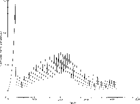
Figure 9.24:
Learning Rate Magnitude as a Function of the Iteration Number for a
Test Problem
The name ``Bold Driver''
was selected for the
analogy with the learning process of young and inexperienced car drivers.
By using this ``brutally heuristic'' method, learning converges in a time
that is comparable to, and usually better than that of standard (batch)
back-propagation with an optimal and fixed learning rate. The
important difference is that the time-consuming
meta-optimization
phase for choosing  is avoided. The values for
  and
and  can be fixed once and for all (e.g.,
  ,
,  )
and performance does not depend critically on their choice.
)
and performance does not depend critically on their choice.
Next:
The Broyden-Fletcher-Goldfarb-Shanno
One-StepMemoryless
Up:
Optimization Methods
for
Previous:
9.9.1 Deficiencies of Steepest
Guy Robinson
Wed Mar 1 10:19:35 EST 1995
The Broyden-Fletcher-Goldfarb-Shanno
One-StepMemoryless Quasi-Newton Method
Next:
9.9.4 Parallel Optimization
Up:
Optimization Methods
for
Previous:
9.9.2 The ``Bold Driver''
Steepest descent suffers from a bad reputation with researchers in
optimization. From the literature (e.g., [
Gill:81a
]), we found a
wide selection of more appropriate optimization
techniques. Following the
``decision tree'' and considering the characteristics of large supervised
learning problems (large memory requirements and time-consuming calculations
of the energy and the gradient), the Broyden-Fletcher-Goldfarb-Shanno
one-step memoryless quasi-Newton method (all adjectives are necessary to
define it) is a good candidate in the competition and performed very
efficiently on different problems.
Let's define the following vectors:  ,
,  and
and
 . The one-dimensional search
direction for the
n
th iteration is a modification of the gradient
. The one-dimensional search
direction for the
n
th iteration is a modification of the gradient
 , as follows:

Every
N
steps (
N
being the number of weights in the network), the search
is restarted in the direction of the negative gradient.
The coefficients  and
and  are combinations of scalar products:

The one-dimensional minimization
used in this
work is based on quadratic
interpolation and tuned to back-propagation where, in a single step, both the
energy value and the negative gradient can be efficiently obtained. Details
on this step are contained in [
Williams:87b
].
The computation during each step requires  operations (the same
behavior as standard batch back-propagation), while the CPU time for
each step increases by an average factor of three for the problems
considered. Because the total number of steps for
convergence
is much smaller, we measured a large net
benefit in computing time.
operations (the same
behavior as standard batch back-propagation), while the CPU time for
each step increases by an average factor of three for the problems
considered. Because the total number of steps for
convergence
is much smaller, we measured a large net
benefit in computing time.
Last but not least, this method can be efficiently implemented on MIMD
parallel computers.
Guy Robinson
Wed Mar 1 10:19:35 EST 1995
9.9.4 Parallel Optimization
Next:
9.9.5 Experiment: the Dichotomy
Up:
Optimization Methods
for
Previous:
The Broyden-Fletcher-Goldfarb-Shanno
One-StepMemoryless
Neural nets are ``by definition'' parallel computing systems of many
densely interconnected units. Parallel computation is the basic method used
by our brain
to achieve response times of hundreds of
milliseconds, using sloppy biological hardware with computing times of
a few milliseconds per basic operation.
Our implementation of the learning algorithm is based on the use of MIMD
machines with large grain size. An efficient mapping strategy consists of
assigning a subset of the examples (input-output pairs) and the
entire
network structure to each processor. To obtain proper
generalization, the number of example patterns has to be much larger (say,
 ) than the number of parameters defining the architecture
(i.e., the number of connection weights). For this reason, the amount
of memory used for storing the weights is not too large for significant
problems.
) than the number of parameters defining the architecture
(i.e., the number of connection weights). For this reason, the amount
of memory used for storing the weights is not too large for significant
problems.
Function and gradient evaluation is executed in parallel. Each processor
calculates the contribution of the assigned patterns (with no communication),
and a global combining-distributing step (see the
ADDVEC
routine in
[
Fox:88a
]) calculates the total energy and gradient (let's remember that
the energy is a
sum
of the patterns' contributions) and communicates
the result to all processors.
Then the one-dimensional minimization along the search direction is completed
and the weights are updated.
Figure 9.25:
``Healthy Food'' Has to Be Distinguished from ``Junk Food'' Using
Taste and Smell Information.
This simple parallelization approach is promising: It can be easily adapted to
different network representations and learning strategies, and it is going to
be a fierce competitor with analog implementations of neural networks, when
these are available for significant applications (let's remember that
airplanes do not flap their wings  ).
).
Guy Robinson
Wed Mar 1 10:19:35 EST 1995
9.9.5 Experiment: the Dichotomy Problem
Next:
9.9.6 Experiment: Time Series
Up:
Optimization Methods
for
Previous:
9.9.4 Parallel Optimization
This problem consists of classifying a set of randomly generated patterns
(with real values) in two classes. An example in two dimensions is given by
the ``healthy food'' learning problem. Inputs are given by points in the
``smell'' and ``taste'' plane, corresponding to the different foods. The
learning task consists of producing the correct classification as ``healthy
food'' or ``junk food'' (Figure
9.25
).
On this problem we obtained a speedup of 20-120 (going from 6 to 100
patterns in two dimensions).
Guy Robinson
Wed Mar 1 10:19:35 EST 1995
9.9.6 Experiment: Time Series Prediction
Next:
9.9.7 Summary
Up:
Optimization Methods
for
Previous:
9.9.5 Experiment: the Dichotomy
In this case, the task is to predict the next value in the sequence (ergodic
and chaotic) generated by the logistic map [
Lapedes:87a
], according to
the recurrence relation:

We tried different architecture and obtained a speedup of 400-500, and
slightly better generalization properties for the BFGS optimization method
presented.
In general, we obtained a larger speedup for problems with high-precision
requirements (using real values for inputs or outputs). See also
[
Battiti:89a
].
Guy Robinson
Wed Mar 1 10:19:35 EST 1995
9.9.7 Summary
Next:
10 DIME Programming Environment
Up:
Optimization Methods
for
Previous:
9.9.6 Experiment: Time Series
The distributed optimization [Battiti:89a;89e]
software was developed by Roberto Battiti,
modifying a back-propagation program written by Steve Otto. Fox and
Williams inspired our first investigations into the
optimization
literature (Shanno's conjugate
gradient
[
Shanno:78a
] is used in
[
Williams:87b
]).
Guy Robinson
Wed Mar 1 10:19:35 EST 1995
10 DIME Programming Environment
Next:
DIME: Portable Software
Up:
Parallel Computing Works
Previous:
9.9.7 Summary
Other References
HPFA Paradigms
Guy Robinson
Wed Mar 1 10:19:35 EST 1995
DIME: Portable Software for IrregularMeshes
for Parallel or SequentialComputers
Next:
10.1.1 Applications and Extensions
Up:
10 DIME Programming Environment
Previous:
10 DIME Programming Environment
In the next two chapters, we describe software tools developed to aid
the user in the parallelization of some of the harder algorithms.
Here we describe DIME,
which is designed to generate both statically
and adaptively irregular meshes. DIME was already used in the
application of Section
7.2
; however, it is more typically
used for partial differential equations describing problems with
nonuniform and varying density.
A large fraction of the problems that we wish to solve with a computer are
continuum simulations of physical systems, where the interesting variable
is not a finite collection of numbers but a function on a domain. For the
purposes of the computation such a continuous spatial domain is given a
structure, or mesh, to which field values may be attached and neighboring
values compared to calculate derivatives of the field.
If the domain of interest has a simple shape, such as a cylinder or cuboid,
there may be a natural choice of mesh
whose structure is very
regular like that of a crystal, but when we come to more complex geometries
such as the space surrounding an aircraft or inside turbomachinery, there are
no regular structures that can adequately represent the domain. The
only way to mesh such complex domains is with an unstructured mesh,
such as that shown in Figure
10.1
. At the right is a plot
of a solution to Laplace's
equation on the domain.
Figure 10.1:
Mesh and Solution of Laplace Equation
Notice that the mesh is especially fine at the sharp corners of the boundary
where the solution changes rapidly: A desirable feature for a mesh is its
ability to adapt, so that when the solution begins to emerge, the mesh
may be made finer where necessary.
Naturally, we would like to run our time-consuming physical simulation
with the most cost-effective general-purpose computer, which we believe to
be the MIMD architecture. In view of the difficulty of programming an
irregular structure such as one of these meshes, and the special difficulty
of doing so with an MIMD machine, I decided to write not just a program for
a specialized application, but a
programming environment
for
unstructured triangular meshes.
The resulting software (DIME: Distributed Irregular Mesh Environment,
[
Williams:90b
]) is responsible for the mesh structure, and a separate
application code runs a particular type of simulation on the mesh. DIME
keeps track of the mesh structure, allowing mesh creation, reading and
writing meshes to disk, and graphics; also adaptive refinement and certain
topological changes to the mesh. It hides the parallelism from the
application code, and splits the mesh among the processors in an efficient
way.
The application code is responsible for attaching data to the elements and
nodes of the mesh, manipulating and computing with these data and the data
from its mesh neighborhood. DIME is designed not only to be portable
between different MIMD parallel machines, but it also runs on any Unix
machine, treating this as a parallel machine with just one processor.
This ability to run on a sequential machine is due to DIME's use of the
Cubix
server (Section
5.2
).
Next:
10.1.1 Applications and Extensions
Up:
10 DIME Programming Environment
Previous:
10 DIME Programming Environment
Guy Robinson
Wed Mar 1 10:19:35 EST 1995
10.1.1 Applications and Extensions
Next:
10.1.2 The Components of
Up:
DIME: Portable Software
Previous:
DIME: Portable Software
The most efficient speed for aircraft flight is just below the speed of
sound: the transonic regime. Simulations of flight at these speeds consume
large quantities of computer time, and are a natural candidate for a DIME
application. In addition to the complex geometries of airfoils and turbines
for which these simulations are required, the flow tends to develop
singular regions or shocks in places that cannot be predicted in
advance; the adaptive refinement
capability of a DIME mesh allows the mesh to be fine and detail
resolved near shocks while keeping the regions of smooth flow coarsely
meshed for economy (Section
12.3
).
The version of DIME developed within C P was only able to mesh
two-dimensional manifolds. More recent developments are described in
Section
10.1.7
. The manifold may, however, be embedded in a
higher-dimensional space. In collaboration with the
Biology
division at Caltech, we have simulated the
electrosensory system of the weakly electric fish
Apteronotus
leptorhynchus
. The simulation involves creating a mesh covering the
skin of the fish, and using the
boundary element method
to
calculate field strengths in the three-dimensional space surrounding
the fish (Section
12.2
).
P was only able to mesh
two-dimensional manifolds. More recent developments are described in
Section
10.1.7
. The manifold may, however, be embedded in a
higher-dimensional space. In collaboration with the
Biology
division at Caltech, we have simulated the
electrosensory system of the weakly electric fish
Apteronotus
leptorhynchus
. The simulation involves creating a mesh covering the
skin of the fish, and using the
boundary element method
to
calculate field strengths in the three-dimensional space surrounding
the fish (Section
12.2
).
In the same vein of embedding the mesh in higher dimensions, we have
simulated a bosonic string of high-energy physics, embedding the mesh in up
to 26 spatial dimensions. The problem here is to integrate over not only all
positions of the mesh nodes, but also over all
triangulations
of the
mesh (Section
7.2
).
The information available to a DIME application is certain data stored
in the elements and nodes of the mesh. When doing
finite-element
calculations, one would like a
somewhat higher level of abstraction, which is to refer to functions
defined on a domain, with certain smoothness constraints and boundary
conditions. We have made a further software layer on top of DIME to
facilitate this: DIMEFEM. With this we may add, multiply,
differentiate and integrate functions defined in terms of the
Lagrangian finite-element family, and define linear, bilinear, and
nonlinear operators acting on these functions. When a bilinear operator
is defined, a variational principle may be solved by
conjugate-gradient
methods. The
preconditioner
for the CG method may in itself
involve solving a variational principle. The DIMEFEM package has been
applied to a sophisticated incompressible flow algorithm
(Section
10.2
).
Next:
10.1.2 The Components of
Up:
DIME: Portable Software
Previous:
DIME: Portable Software
Guy Robinson
Wed Mar 1 10:19:35 EST 1995
10.1.2 The Components of DIME
Next:
10.1.3 Domain Definition
Up:
DIME: Portable Software
Previous:
10.1.1 Applications and Extensions
Figure
10.2
shows the structure of a DIME application. The shaded
parts represent the contribution from the user, being a definition of a
domain which is to be meshed, a definition of the data to be maintained at
each element, node, and boundary edge of the mesh, and a set of functions
that manipulate this data. The user may also supply or create a script file
for running the code in batch mode.
Figure 10.2:
Major Components of DIME
The first input is the definition of a domain to be meshed. A file may be
made using the elementary CAD program
curvetool
, which allows straight
lines, arcs, and cubic splines to be manipulated interactively to define a
domain.
Before sending a domain to a DIME application, it must be predigested to some
extent, with the help of a human. The user must produce a coarse mesh that
defines the topology of the domain to the machine. This is done with the
program
meshtool
, which allows the user to create nodes and connect
them to form a triangulation.
The user writes a program for the mesh, and this program is loaded into each
processor of the parallel machine. When the DIME function
readmesh
()
is called, (or ``Readmesh'' clicked on the menu), the mesh created by
meshtool
is read into a single processor, and then the function
balance_orb
() may be called (or ``Balance'' clicked on the menu) to
split the mesh into domains, one domain for each processor.
The user may also call the function
writemesh
() (or click
``Writemesh'' in the menu), which causes the parallel mesh to be written to
disk. If that mesh is subsequently read in, it is read in its
domain-decomposed form, with different pieces assigned to different
processors.
In Figure
10.2
, the Cubix
server is not
mandatory, but only needed if the DIME application is to run in
parallel. The application
also runs on a sequential machine
,
which is considered to be a one-processor parallel machine.
Next:
10.1.3 Domain Definition
Up:
DIME: Portable Software
Previous:
10.1.1 Applications and Extensions
Guy Robinson
Wed Mar 1 10:19:35 EST 1995
10.1.3 Domain Definition
Next:
10.1.4 Mesh Structure
Up:
DIME: Portable Software
Previous:
10.1.2 The Components of
Figure
10.3
shows an example of a DIME boundary structure. The
filled blobs are
points
, with
curves
connecting the points. Each
curve may consist of a set of curve segments, shown in the figure separated
by open circles. The curve segments may be straight lines, arcs of circles,
or Bezier cubic sections. The program
curvetool
is for the interactive
production of boundary files. When the domain is satisfactory, it should be
meshed using
meshtool
.
Figure 10.3:
Boundary Structure
The program
meshtool
is used for defining boundaries and creating
a triangulation of certain regions of a grid.
Meshtool
adds
nodes to an existing triangulation using the Delaunay
triangulation
[
Bowyer:81a
]. A new
node may be added anywhere except at the position of an existing node.
Figure
10.4
illustrates how the Delaunay triangulation
(thick gray lines) is derived from the Voronoi tesselation (thin black
lines).
Figure 10.4:
Voronoi Tesselation and Resulting Delaunay Triangulation
Each node (shown by a blob in the figure) has a ``territory,'' or Voronoi
polygon, which is the part of the plane closer to the node than to any other
node. The divisions between these territories are shown as thin lines in the
figure, and are the perpendicular bisectors of the lines between the nodes.
This procedure tesselates the plane into a set of disjoint polygons and is
called the Voronoi tesselation. Joining nodes whose Voronoi polygons have a
common border creates a triangulation of the nodes known as the Delaunay
triangulation. This triangulation has some desirable properties, such as the
diagonal dominance of a finite-element
stiffness
matrix derived from the mesh [
Young:71a
].
Guy Robinson
Wed Mar 1 10:19:35 EST 1995
10.1.4 Mesh Structure
Next:
10.1.5 Refinement
Up:
DIME: Portable Software
Previous:
10.1.3 Domain Definition
Figure
10.5
shows a triangular mesh covering a rectangle, and
Figure
10.6
the logical structure of that mesh split among four
processors. The logical mesh shows the elements as shaded triangles and nodes
as blobs. Each element is connected to exactly three nodes, and each node is
connected to one or more elements. If a node is at a boundary, it has a
boundary structure attached, together with a pointer to the next node
clockwise around the boundary.
Figure 10.5:
A Mesh Covering a Rectangle
Figure 10.6:
The Logical Structure of the Mesh Split Among Four Processors
Each node, element and boundary structure has user data attached to it, which
is automatically transferred to another processor if load-balancing causes the
node or element to be moved to another processor. DIME knows only the size
of the user data structures. Thus, these structures may not contain pointers,
since when those data are moved to another processor the pointers will be
meaningless.
The shaded ovals in Figure
10.5
are
physical nodes
,
each of which consists of one or more
logical nodes
. Each logical
node has a set of aliases, which are the other logical nodes belonging
to the same physical node. The physical node is a conceptual object,
and is unaffected by parallelism; the logical node is a copy of the
data in the physical node, so that each processor which owns a part of
that physical node may access the data as if it had the whole node.
DIME is meant to make distributed processing of an unstructured
mesh
almost
as easy as sequential programming. However, there is a remaining ``kernel
of parallelism'' that the user must bear in mind. Suppose each node of the
mesh gathers data from its local environment (i.e., the neighboring
elements); if that node is split among several processors, it will only
gather the data from those elements which lie in the same processor and
consequently each node will only have part of the result. We need to combine
the partial results from the logical nodes and return the combined result to
each. This facility is provided by a macro in DIME called
NODE_COMBINE
, which is called each time the node data is changed
according to its local environment.
Next:
10.1.5 Refinement
Up:
DIME: Portable Software
Previous:
10.1.3 Domain Definition
Guy Robinson
Wed Mar 1 10:19:35 EST 1995
10.1.5 Refinement
Next:
10.1.6 Load Balancing
Up:
DIME: Portable Software
Previous:
10.1.4 Mesh Structure
The Delaunay triangulation used by
meshtool
would be an ideal way to
refine the working mesh, as well as making a coarse mesh for initial
download. Unfortunately, adding a new node to an existing Delaunay
triangulation may have global consequences; it is not possible to predict
in advance how much of the current mesh should be replaced to accommodate the
new node. Doing this in parallel requires an enormous amount of communication
to make sure that the processors do not tread on each others' toes
[
Williams:89c
].
DIME uses the algorithm of Rivara [Rivara:84a;89a]
for refinement of the mesh, which is well suited to
loosely synchronous parallel operation, but results in a triangulation
which is not a Delaunay triangulation, and thus lacks some desirable
properties. The process of topological relaxation changes the
connectivity of the mesh to make it a Delaunay triangulation.
It is usually desirable to avoid triangles in the mesh which have
particularly acute angles, and topological relaxation will reduce this
tendency. Another method of doing this is by moving the nodes toward
the average position of their neighboring nodes; a physical analogy
would be to think of the edges of the mesh as damped springs and
allowing the nodes to move under the action of the springs.
Guy Robinson
Wed Mar 1 10:19:35 EST 1995
10.1.6 Load Balancing
Next:
10.1.7 Summary
Up:
DIME: Portable Software
Previous:
10.1.5 Refinement
When DIME operates in parallel, the mesh should be distributed among the
processors of the machine so that each processor has about the same amount of
mesh to deal with, and the communication time is as small as
possible. There are several ways to do this, such as with a computational
neural net, by simulated annealing,
or even
interactively.
DIME uses a strategy known as
recursive bisection
[
Fox:88mm
], which has the advantages of being robust,
simple, and deterministic, though sometimes the resulting communication
pattern may be less than optimal. The method is illustrated in
Figure
10.7
: each blob represents the center of an
element, and the vertical and horizontal lines represent processor
divisions. First, a median vertical line is found which splits the set
of elements into two sets of approximately equal numbers, then (with
two-way parallelism) two horizontal medians which split the halves into
four approximately equal quarters, then (with four-way parallelism)
four vertical medians, and so on. Chapter
11
describes more
general and powerful load-balancing methods.
Figure 10.7:
Recursive Bisection
Figure 10.8 (Color Plate) and Figure 10.9 (Color Plate) are from a calculation
of transonic flow over an airfoil (see Section
12.3
).
Figure 10.9 shows the parallel structure of the DIME mesh
used to calculate the flow. The redundant copies of shared nodes have
been separated to show the data connections between them in yellow and
blue.
Figure :
Pressure plot Mach 0.8 flow over a NACA0012
airfoil, with the sonic line shown. The mesh for this computation is shown
in Figure 10.9.
Figure 10.9:
Depiction of the mesh for the transonic
flow calculation of color Figure 10.8. Each group of similarly colored
triangles is owned by an individual processor. The mesh has been
dynamically adapted and load-balanced. The yellow lines connect copies of
nodes which are in the same geometric positioin, but have been separated
for the purpose of this picture. The load balancing is by orthogonal
recursive bisection.
In the pressure plot, there is a vertical shock about two-thirds of the
way downstream from the leading edge of the airfoil. This can also be
seen in the mesh plot since the same region has especially small
triangles and high mesh density. Since each processor has about the
same number of triangles, the processor regions are also small in the
neighborhood of the shock.
Next:
10.1.7 Summary
Up:
DIME: Portable Software
Previous:
10.1.5 Refinement
Guy Robinson
Wed Mar 1 10:19:35 EST 1995
10.1.7 Summary
Next:
DIMEFEM: High-level Portable
Up:
DIME: Portable Software
Previous:
10.1.6 Load Balancing
The DIME software was written by Roy Williams, and the C P work is
published in [
Baillie:90e
], [Williams:87a;87b;88a;88d;89c;90b].
P work is
published in [
Baillie:90e
], [Williams:87a;87b;88a;88d;89c;90b].
DIME has evolved recently into something rather more general: instead
of a set of explicitly triangular elements which have access to the
three nodes around them, the new language DIME++ has the idea of a set
of objects that have an index to another set of objects. Just as DIME
is able to refine its mesh dynamically, and load-balance the mesh, so
in DIME++ the indices may be created and modified dynamically and the
sets load-balanced [Williams:91a;91c;92a;93b].
This more general formulation of the interface frees the system from
explicitly triangular meshes, and greatly expands and generalizes the
range of problems that can be addressed: higher dimensions,
different kinds of elements, multigrid, graph problems, and
multiblock. Instead of linked lists,
DIME++ stores
data in long vectors for maximum efficiency; it is written as a C++
class library for extensibility and polymorphism.
Guy Robinson
Wed Mar 1 10:19:35 EST 1995
DIMEFEM: High-level Portable Irregular-Mesh
Finite-Element Solver
Next:
10.2.1 Memory Allocation
Up:
10 DIME Programming Environment
Previous:
10.1.7 Summary
DIMEFEM
[
Williams:89a
] is a software layer which
enables finite-element
calculations to be done
with the irregular mesh maintained by DIME. The data objects dealt
with by DIMEFEM are finite-element functions (FEFs), which may be
scalar or have several components (vector fields), as well as linear,
multilinear and nonlinear operators which map these FEFs to numbers.
The guiding principle is that interesting physical problems may be
expressed in variational terms involving FEFs and operators on them
[
Bristeau:87a
], [
Glowinski:84a
]. We shall use as an example
a Poisson solver.
Poisson's equation is  , which may also be expressed
variationally as: Find
u
such that for all
v
, which may also be expressed
variationally as: Find
u
such that for all
v

where the unknown
u
and the dummy variable
v
are taken to have the
correct boundary conditions. To implement this with DIMEFEM, we first
allocate space in each element for the FEFs
u
and
f
, then explicitly set
f
to the desired function. We now define the linear operator
L
and
bilinear operator
a
as above, and call the linear solver to evaluate
u
.
Guy Robinson
Wed Mar 1 10:19:35 EST 1995
10.2.1 Memory Allocation
Next:
10.2.2 Operations and Elements
Up:
DIMEFEM: High-level Portable
Previous:
DIMEFEM: High-level Portable
When DIME creates a new element by refinement, it comes equipped with a
pointer to a block of memory of user-specified size which DIMEFEM uses
to store the data representing FEFs and corresponding linear operators.
A template is kept of this element memory containing information about
which one is already allocated and which one is free. When an FEF is to
be created, the memory allocator is called, which decides how much
memory is needed per element and returns an offset from the start of
the element-data-space for storing the new FEF. Thus, a function in
DIMEFEM typically consists of allocating a stack of work space, doing
calculations, then freeing the work space.
An FEF thus consists of a specification of an element type, a number of
fields (one for scalar, two or more for vector), and an offset into the
element data for the nodal values.
Guy Robinson
Wed Mar 1 10:19:35 EST 1995
10.2.2 Operations and Elements
Next:
10.2.3 Navier-Stokes Solver
Up:
DIMEFEM: High-level Portable
Previous:
10.2.1 Memory Allocation
Finite-element approximations to functions form a finite-dimensional vector
space, and as such may be multiplied by a scalar and added. Functions are
provided to do these operations. If the function is expressed as Lagrangian
elements it may also be differentiated, which changes the order of
representation: For example, differentiating a quadratic element produces a
linear element.
At present, DIMEFEM provides two kinds of elements, Lagrangian and Gaussian,
although strictly speaking the latter is not a finite element because it
possesses no interpolation functions. The Gaussian element is simply a
collection of function values at points within each triangle and a set of
weights, so that integrals may be done by summing the function values
multiplied by the weights. As with one-dimensional Gaussian integration,
integrals are exact to some polynomial
order. We cannot differentiate Gaussian FEFs, but can apply pointwise
operators such as multiplication and function evaluation that cannot be
done in the Lagrangian representation.
Consider the nonlinear operator
L
defined by

The most accurate way to evaluate this is to start with
u
in Lagrangian
form, differentiate, convert to Gaussian representation, exponentiate, then
multiply by the weights and sum. This can be done explicitly with DIMEFEM,
but in the future we hope to create an environment which ``knows'' about
representations, linearity, and so on, and can parse an expression such as the
above and evaluate it correctly.
The computational kernel of any finite-element software is the linear solver.
We have implemented this with preconditioned conjugate
gradient
, so that the user supplies a linear
operator
L
, an elliptic bilinear operator
a
, a scalar product
S
(a strongly elliptic symmetric bilinear operator which satisfies
the triangle inequality), and an initial guess for the solution. The
conjugate-gradient
solver replaces the guess
by the solution
u
of the standard variational equation

using the preconditioner
S
.
Next:
10.2.3 Navier-Stokes Solver
Up:
DIMEFEM: High-level Portable
Previous:
10.2.1 Memory Allocation
Guy Robinson
Wed Mar 1 10:19:35 EST 1995
10.2.3 Navier-Stokes Solver
Next:
10.2.4 Results
Up:
DIMEFEM: High-level Portable
Previous:
10.2.2 Operations and Elements
We have implemented a sophisticated incompressible flow solver using DIME and
DIMEFEM. The algorithm is described more completely in
[
Bristeau:87a
]. The evolution equation for an incompressible Newtonian
fluid of viscosity
n
is

We use a three-stage operator-split scheme whereby for each time step of
length
dt
, the equation is integrated
-
from
t
to
 with incompressibility and no convection,
then
with incompressibility and no convection,
then
-
from
 to
to  with convection and
no incompressibility condition, then
with convection and
no incompressibility condition, then
-
to
t + dt
as in stage one with incompressibility and no convection.
The parameter  is
is  .
.
Each of these three implicit steps involves the solution of either a Stokes
problem:

or the nonlinear problem:\

where  is a parameter inversely proportional to the time step. We
solve the Navier-Stokes equation,
and
consequently also these subsidiary problems, with given velocity at the
boundary (Dirichlet boundary conditions).
is a parameter inversely proportional to the time step. We
solve the Navier-Stokes equation,
and
consequently also these subsidiary problems, with given velocity at the
boundary (Dirichlet boundary conditions).
Guy Robinson
Wed Mar 1 10:19:35 EST 1995
10.2.4 Results
Next:
10.2.5 Summary
Up:
DIMEFEM: High-level Portable
Previous:
10.2.3 Navier-Stokes Solver
With velocity approximated by quadratic, and pressure by linear Lagrangian
elements, we found that both the Stokes and nonlinear solvers converged in
three to five iterations. We ran the square cavity problem
as a benchmark.
To reach a steady-state solution, we adopted the following strategy:
With a coarse mesh, keep advancing simulation time until the velocity field no
longer changes, then refine the mesh, iterate until the velocity stabilizes,
refine, and so on. The refinement strategy was as follows. The velocity is
approximated with quadratic elements with discontinuous derivatives, so we
can calculate the maximum of this derivative discontinuity for each element,
then refine those elements above the 70th percentile of this quantity.
Figure
10.10
shows the results. At top left is the mesh
after four cycles of this refinement and
convergence
, at Reynolds number 1000. We note heavy
refinement at the top left and top right, where the boundary conditions
force a discontinuity in velocity, and also along the right side where
the near discontinuous vorticity field is being transported around the
primary vortex. Bottom left shows the logical structure, split among
four transputers.
The top right and bottom right
show streamlines and vorticity, respectively. The results accord well
with the benchmark of [
Schreiber:83a
].
Figure 10.10:
Results for Square Cavity Problem with Reynolds Number 1000
Guy Robinson
Wed Mar 1 10:19:35 EST 1995
10.2.5 Summary
Next:
11 Load Balancing and
Up:
DIMEFEM: High-level Portable
Previous:
10.2.4 Results
The DIMEFEM software was written by Roy Williams, and the flow algorithm
developed by R. Glowinski of the University of Houston [Williams:89a;90b].
Guy Robinson
Wed Mar 1 10:19:35 EST 1995
11 Load Balancing and Optimization
Next:
11.1 Load Balancing as
Up:
Parallel Computing Works
Previous:
10.2.5 Summary
Guy Robinson
Wed Mar 1 10:19:35 EST 1995
11.1 Load Balancing as an Optimization Problem
Next:
11.1.1 Load Balancing a
Up:
11 Load Balancing and
Previous:
11 Load Balancing and
We have seen many times that parallel computing involves breaking
problems into parts which execute concurrently. In the simple regular
problems seen in the early chapters, especially Chapters
4
and
6
, it was usually reasonably obvious how to
perform this breakup to optimize performance of the program on a
parallel machine. However, in Chapter
9
and even more so in
Chapter
12
, we will find that the nature of the parallelism is
as clear as before, but that it is nontrivial to implement
efficiently.
Irregular loosely synchronous problems consist of a collection of
heterogeneous tasks communicating with each other at the
macrosynchronization points characteristic of this problem class. Both
the execution time per task and amount and pattern of communication can
differ from task to task. In this section, we describe and compare
several approaches to this problem. We note that formally this is a
very hard-so-called NP-complete-optimization problem. With
 tasks running on
  processors we
cannot afford to examine every one of the
processors we
cannot afford to examine every one of the 
 assignments
of tasks to processors.
Experience has shown that this problem is easier than one would have
thought-partly at least because one does not require the exactly
optimal assignment. Rather, a solution whose execution time is, say,
within 10% of the optimal value is quite acceptable. Remember, one
has probably chosen to ``throw away'' a larger fraction than this of
the possible MPP performance by using a high-level language such as
Fortran or C on the node (independent of any parallelism issues). The
physical optimization
methods described in Section
11.3
and more problem-specific
heuristics
have shown themselves very suitable for
this class of approximate optimization [Fox:91j;92i].
In 1985, at a DOE contract renewal review at Caltech,
we thought that this load balancing issue would be a major and perhaps
the key stumbling block for parallel computing. However, this is not
the case-it is a hard and important problem, but for loosely
synchronous problems it can be solved straightforwardly
[
Barnard:93a
], [Fox:92c;92h;92i],
[
Fox:92h
] [
Mansour:92d
]. Our approach to
this uses physical analogies and stems in fact from dinner
conversations between Fox and David Jefferson, a collaborator from
UCLA, at this meeting
[Fox:85k;86a;88e;88mm]. An
interesting computer science challenge is to understand why the
NP-complete
load-balancing problem appears ``easier
in practice'' than the Travelling Salesman Problem, which is the
generic NP-complete optimization problem. We will return to this
briefly in Section
11.3
, but note that the ``shape of the
objection function'' (in physics language, the ``energy landscape'')
illustrated in Figure
11.1
appears critical. Load-balancing
problems appear to fall into the ``easy class'' of NP-complete
optimization problems with the landscape of Figure
11.1
(a).
The methods discussed in the following are only a sample of the many
effective approaches developed recently: [
Barhen:88a
],
[
Berger:87a
], [
Chen:88a
], [
Chrisochoides:91a
],
[
Ercal:88a
], [
Ercal:88b
],
[Farhat:88a;89b], [
Fox:88nn
],
[
Hammond:92b
], [
Houstis:90a
], [
Livingston:88a
],
[
Miller:92a
], [
Nolting:91a
], [
Teng:91a
],
[
Walker:90b
]. The work of Simon [
Barnard:93a
],
[
Pothen:90a
], [
Simon:91b
], [
Venkatakrishnan:92a
] on
recursive spectral bisection-a method with similarities to the
eigenvector recursive bisection
(ERB) method mentioned later-has
been particularly successful.
assignments
of tasks to processors.
Experience has shown that this problem is easier than one would have
thought-partly at least because one does not require the exactly
optimal assignment. Rather, a solution whose execution time is, say,
within 10% of the optimal value is quite acceptable. Remember, one
has probably chosen to ``throw away'' a larger fraction than this of
the possible MPP performance by using a high-level language such as
Fortran or C on the node (independent of any parallelism issues). The
physical optimization
methods described in Section
11.3
and more problem-specific
heuristics
have shown themselves very suitable for
this class of approximate optimization [Fox:91j;92i].
In 1985, at a DOE contract renewal review at Caltech,
we thought that this load balancing issue would be a major and perhaps
the key stumbling block for parallel computing. However, this is not
the case-it is a hard and important problem, but for loosely
synchronous problems it can be solved straightforwardly
[
Barnard:93a
], [Fox:92c;92h;92i],
[
Fox:92h
] [
Mansour:92d
]. Our approach to
this uses physical analogies and stems in fact from dinner
conversations between Fox and David Jefferson, a collaborator from
UCLA, at this meeting
[Fox:85k;86a;88e;88mm]. An
interesting computer science challenge is to understand why the
NP-complete
load-balancing problem appears ``easier
in practice'' than the Travelling Salesman Problem, which is the
generic NP-complete optimization problem. We will return to this
briefly in Section
11.3
, but note that the ``shape of the
objection function'' (in physics language, the ``energy landscape'')
illustrated in Figure
11.1
appears critical. Load-balancing
problems appear to fall into the ``easy class'' of NP-complete
optimization problems with the landscape of Figure
11.1
(a).
The methods discussed in the following are only a sample of the many
effective approaches developed recently: [
Barhen:88a
],
[
Berger:87a
], [
Chen:88a
], [
Chrisochoides:91a
],
[
Ercal:88a
], [
Ercal:88b
],
[Farhat:88a;89b], [
Fox:88nn
],
[
Hammond:92b
], [
Houstis:90a
], [
Livingston:88a
],
[
Miller:92a
], [
Nolting:91a
], [
Teng:91a
],
[
Walker:90b
]. The work of Simon [
Barnard:93a
],
[
Pothen:90a
], [
Simon:91b
], [
Venkatakrishnan:92a
] on
recursive spectral bisection-a method with similarities to the
eigenvector recursive bisection
(ERB) method mentioned later-has
been particularly successful.
Figure 11.1:
Two Possible ``Energy Landscapes'' for an Optimization
Problem
A few general remarks are necessary; we use the phrases ``load
balancing'' and ``data decomposition'' interchangeably. One needs
both
ab initio
and dynamic distribution and redistribution of data on
the parallel machine. We also can examine load balancing at the level
of data or of tasks that encapsulate the data and
algorithm. In elegant (but currently inefficient) software models
with one datum per task, these formulations are equivalent. Our
examples will do load balancing at the level of data values, but the
task and data distribution problems are essentially equivalent.
Our methods are applicable to general loosely synchronous problems and
indeed can be applied to arbitrary problem classes. However, we will
choose a particular finite-element problem to illustrate the issues
where one needs to distribute a mesh, such as that illustrated in
Figure
11.2
. Each triangle or element represents a task
which communicates with its neighboring three triangles. In doing, for
example, a simulation of fluid flow on the mesh, each element of the
mesh communicates regularly with its neighbors, and this pattern may be
repeated thousands of times.
Figure 11.2:
An Unstructured Triangular Mesh Surrounding a Four-Element
Airfoil. The mesh is distributed among 16 processors, with divisions
shown by heavy lines.
We may classify load-balancing strategies into four broad types, depending on
when the optimization is made and whether the cost of the optimization is
included in the optimization itself:\
-
By Inspection:
The load-balancing strategy may be determined
by inspection, such as with a rectangular lattice of grid points split into
smaller rectangles, so that the load-balancing problem is solved before the
program is written. This is illustrated by the QCD decomposition of
Figure
4.3
.
-
Static:
The optimization is nontrivial, but may be done by
a sequential machine before starting the parallel program, so that the
load-balancing problem is solved before the parallel program begins.
-
Quasi-Dynamic:
The circumstances determining the optimal balance
change during program execution, but discretely and infrequently. Because
the change is discrete, the load-balance
problem,
and hence its solution, remain the same until the next change. If
these changes are infrequent enough, any savings made in the subsequent
computation make up for the time spent solving the load-balancing
problem. The difference between this and the static case is that the
load balancing must be carried out in parallel to prevent a sequential
bottleneck.
Koller calls these problems
adiabatic
[
Fox:90nn
], using a physical
analogy where the load balancer can be viewed as a heatbath keeping
the problem in equilibrium. In adiabatic systems, changes are
sufficiently slow that the heatbath can ``keep up'' and the system
evolves from equilibrium state to equilibrium state.
-
Dynamic:
The circumstances determining the optimal
balance change frequently or continuously during execution, so that the
cost of the load balancing calculation after each change should be
minimized in addition to optimizing the splitting of the actual
calculation. This means that there must be a decision made every so
often to decide if load balancing is necessary, and how much time to
spend on it. The chess program in Section
14.3
shows very
irregular dynamic behavior so that statistical load-balancing methods
similar to the
scattered
decomposition of Section
11.2
must be used.
If the mesh is solution-adaptive, that is, if the mesh, and hence the
load-balancing problem, change discretely during execution of the code,
then it is most efficient to decide the optimal mesh distribution in
parallel. In this section, three parallel algorithms,
orthogonal
recursive bisection
(ORB),
eigenvector
recursive bisection
(ERB) and a
simple parallelization of
simulated annealing
(SA) are discussed for load-balancing a dynamic
unstructured triangular mesh on 16 processors of an nCUBE
machine.
The test problem is a solution-adaptive Laplace
solver, with an initial mesh of 280 elements, refined in seven stages
to 5772 elements. We present execution times for the solver resulting
from the mesh distributions using the three algorithms, as well as
results on imbalance, communication traffic, and element migration.
In this section, we shall consider the quasi-dynamic case with observations
on the time taken to do the load balancing that bear on the dynamic case.
The testbed is an unstructured-mesh finite-element code, where the elements
are the atoms of the problem, which are to be assigned to processors. The
mesh is solution-adaptive, meaning that it becomes finer in places where the
solution of the problem dictates refinement.
We shall show that a class of finite-element applications share common
load-balancing requirements, and formulate load balancing as a graph-coloring
problem. We shall discuss three methods for solving this graph-coloring
problem: one based on statistical physics, one derived from a computational
neural net, and one cheap and simple method.
We present results from running these three load-balancing methods, both in
terms of the quality of the graph-coloring solution (machine-independent
results), and in terms of the particular machine (16 processors of an nCUBE)
on which the test was run.
Next:
11.1.1 Load Balancing a
Up:
11 Load Balancing and
Previous:
11 Load Balancing and
Guy Robinson
Wed Mar 1 10:19:35 EST 1995
11.1.1 Load Balancing a Finite-Element Mesh
Next:
11.1.2 The Optimization Problem
Up:
11.1 Load Balancing as
Previous:
11.1 Load Balancing as
An important class of problems are those which model a continuum system by
discretizing continuous space with a mesh. Figure
11.2
shows an
unstructured triangular mesh surrounding a cross-section of a four-element
airfoil from an Airbus A-310. The variations in mesh density are caused by
the nature of the calculation for which the mesh has been used; the airfoil
is flying at Mach 0.8 to the left, so that a vertical shock extends upward at
the trailing edge of the main airfoil, which is reflected in the increased
mesh density.
The mesh has been split among 16 processors of a distributed machine, with
the divisions between processors shown by heavy lines. Although the areas of
the processor domains are different, the numbers of triangles or elements
assigned to the processors are essentially the same. Since the work done by
a processor in this case is the same for each triangle, the workloads for the
processors are the same. In addition, the elements have been assigned to
processors so that the number of adjacent elements which are in different
processors is minimized.
In order to analyze the optimal distribution of elements among the
processors, we must consider the way the processors need to exchange data
during a calculation. In order to design a general load balancer for such
calculations, we would like to specify this behavior with the fewest possible
parameters, which do not depend on the particular mesh being distributed.
The following remarks apply to several application codes,
written to run with the DIME software (Section
10.1
), which use
two-dimensional unstructured meshes, as follows:\
-
Laplace:
A scalar Laplace solver with linear finite elements,
using Jacobi relaxation;
-
Wing:
A finite-volume transonic Euler solver, with harmonic and
biharmonic artificial dissipation [
Williams:89b
];
-
Convect:
A simple finite-volume solver which convects a scalar
field with uniform velocity, with no dissipation;
-
Stress:
A plane-strain elasticity solver with linear finite
elements using conjugate gradient
to solve the
stiffness matrix;
-
Fluid:
An incompressible flow solver with quadratic elements
for velocity and linear elements for pressure, using conjugate
gradient
to solve the Stokes problem and a nonlinear
least-squares technique for the convection [
Williams:89a
].
As far as load balancing is concerned, all of these codes are rather
similar. This is because the algorithms used are local: Each
element or node of the mesh gets data from its neighboring elements or
nodes. In addition, a small amount of global data is needed; for
example, when solving iteratively, each processor calculates the norm of
the residual over its part of the mesh, and all the processors need the
minimum value of this to decide if the solve has converged.
We can analyze the performance of code using an approach similar to that
in Section
3.5
. In this case, the computational kernel of
each of these applications is iterative, and each iteration may be
characterized by three numbers:\
-
the number of floating-point operations during the iteration, which is
proportional to the number of elements (or nodes or mesh points) owned
by the processor;
-
the number of global combining operations during the iteration;
-
the number and size of local communication events, in which the
elements at the boundary of the processor region communicate data loosely
synchronously [
Fox:88a
] with their neighboring elements in other
processors, which is proportional to the number of elements at the boundary
of the processor domain.
These numbers are listed in the following table for the five applications
listed above:\
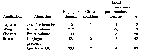
The two finite-volume applications do not have iterative matrix solves,
so they have no convergence
checking and thus have
no need for any global data exchange. The ratio
c
in the last column
is the ratio of the third to the fifth columns and may be construed as
follows. Suppose a processor has
E
elements, of which
B
are at the
processor boundary. Then the amount of communication the processor
must do compared to the amount of calculation is given by the general
form of Equation
3.10
, which here becomes

It follows that a large value of
c
corresponds to an eminently
parallelizable operation, since the communication rate is low compared to
calculation. The ``Stress'' example has a high value of
c
because the
solution being sought is a two-dimensional strain field; while the
communication is doubled, the calculation is quadrupled, because the elements
of the scalar stiffness matrix are replaced by  block matrices,
and each block requires four multiplies instead of one. For the ``Fluid''
example, with quadratic elements, there are the two components of velocity
being communicated at both nodes and edges, which is a factor of four for
communication, but the local stiffness matrix is now
block matrices,
and each block requires four multiplies instead of one. For the ``Fluid''
example, with quadratic elements, there are the two components of velocity
being communicated at both nodes and edges, which is a factor of four for
communication, but the local stiffness matrix is now  because
of the quadratic elements. Thus, we conclude that the more interacting
fields, and the higher the element order, the more efficiently the
application runs in parallel.
because
of the quadratic elements. Thus, we conclude that the more interacting
fields, and the higher the element order, the more efficiently the
application runs in parallel.
Next:
11.1.2 The Optimization Problem
Up:
11.1 Load Balancing as
Previous:
11.1 Load Balancing as
Guy Robinson
Wed Mar 1 10:19:35 EST 1995
11.1.2 The Optimization Problem and Physical Analogy
Next:
11.1.3 Algorithms for Load
Up:
11.1 Load Balancing as
Previous:
11.1.1 Load Balancing a
We wish to distribute the elements among the processors of the machine to
minimize both load imbalance (one processor having more elements than
another) and communication between elements.
Our approach here is to write down a cost function
which is minimized when the total running time of the code is minimized
and is reasonably simple and independent of the details of the code.
We then minimize this cost function and distribute the elements
accordingly.
The load-balancing problem [Fox:88a;88mm],
may be stated as a graph-coloring
problem: Given an
undirected graph of
N
nodes (finite elements), color these nodes with
P
colors (processors) to minimize a cost function
H
which is
related to the time taken to execute the program for a given coloring.
For DIME applications, it is the finite elements which are to be
distributed among the processors, so the graph to be colored is
actually the dual graph to the mesh, where each graph node corresponds
to an element of the mesh and has (if it is not at a boundary) three neighbors.
We may construct the cost function as the sum of a part that minimizes
load imbalance and one that minimizes communication:\

where  is the part of the cost function which is minimized when
each processor has equal work,
is the part of the cost function which is minimized when
each processor has equal work,  is minimal when communication time
is minimized, and
is minimal when communication time
is minimized, and  is a parameter expressing the balance between the
two, with
is a parameter expressing the balance between the
two, with  related to the number
c
discussed above. If
related to the number
c
discussed above. If  and
and  were proportional to the times taken for calculation and
communication, then
were proportional to the times taken for calculation and
communication, then  should be inversely proportional to
c
. For
programs with a great deal of calculation compared to communication,
should be inversely proportional to
c
. For
programs with a great deal of calculation compared to communication,
 should be small, and vice versa.
As  is increased, the number of processors in use will decrease until
eventually the communication is so costly that the entire calculation must be
done on a single processor.
is increased, the number of processors in use will decrease until
eventually the communication is so costly that the entire calculation must be
done on a single processor.
Let
e, f,
 label the nodes of the graph, and
  be the
color (or processor assignment) of graph node
e
. Then the number of graph
nodes of color
q
is:\
be the
color (or processor assignment) of graph node
e
. Then the number of graph
nodes of color
q
is:\

and  is proportional to the maximum value of
  , because the
whole calculation runs at the speed of the slowest processor, and the slowest
processor is the one with the most graph nodes. This ignores node and
link (node-to-node communication) contention, which contribute to idle
time.
, because the
whole calculation runs at the speed of the slowest processor, and the slowest
processor is the one with the most graph nodes. This ignores node and
link (node-to-node communication) contention, which contribute to idle
time.
The formulation as a maximum of  is, however, not satisfactory
when a perturbation is added to the cost function, such as that from
the communication cost function. If, for example, we were to add a
linear forcing term proportional to
is, however, not satisfactory
when a perturbation is added to the cost function, such as that from
the communication cost function. If, for example, we were to add a
linear forcing term proportional to  , the cost function would be:\

and the minimum of this perturbed cost function is either  if
if  is less than
  , or
, or  ,
,
 if
if  is larger than this. This
discontinuous behavior as a result of perturbations is undesirable, so
we use a sum of squares instead, whose minima change smoothly with the
magnitude of a perturbation:\
is larger than this. This
discontinuous behavior as a result of perturbations is undesirable, so
we use a sum of squares instead, whose minima change smoothly with the
magnitude of a perturbation:\

where  is a scaling constant to be determined.
We now consider the communication part of the cost function. Let
us define the matrix

which is the amount of communication between processors
q
and
r
, and the notation  means that the graph nodes
e
and
f
are connected by an edge of the graph.
means that the graph nodes
e
and
f
are connected by an edge of the graph.
The cost of communication from processors
q
to
r
depends on the
machine architecture; for some parallel machines it may be possible to write
down this metric explicitly. For example, with the early hypercubes, the cost
is the number of bits which are different in the binary representations of
the processor numbers
q
and
r
. The metric may also depend on the
message-passing software, or even on the activities of other users for a
shared machine. A truly portable load balancer would have no option but to
send sample messages around and measure the machine metric, then distribute
the graph appropriately. In this book, however, we shall avoid the question
of the machine metric by simply assuming that all pairs of processors are
equally far apart, except of course a processor may communicate with itself
at no cost.
The cost of sending the quantity  of data also depends on the
programming: the cost will be much less if it is possible for the
of data also depends on the
programming: the cost will be much less if it is possible for the
 messages to be bundled together and sent as one, rather
than separately. The major problem is latency:
The
cost to send a message in any distributed system is the sum of an
initial fixed price and one proportional to the size of the
message. This is also the case for the pricing of telephone calls,
freight shipping, mail service, and many other examples from the
everyday world. If the message is large enough, we may ignore
latency: For the nCUBE used in Section
11.1.7
of this book,
latency may be ignored if the message is longer than a hundred bytes or
so. In the tests of Section
11.1.7
, most of the messages are
indeed long enough to neglect latency, though there is certainly
further work needed on load balancing in the presence of this important
effect. We also ignore blocking (idling) due to needed resources
being unavailable due to contention.
messages to be bundled together and sent as one, rather
than separately. The major problem is latency:
The
cost to send a message in any distributed system is the sum of an
initial fixed price and one proportional to the size of the
message. This is also the case for the pricing of telephone calls,
freight shipping, mail service, and many other examples from the
everyday world. If the message is large enough, we may ignore
latency: For the nCUBE used in Section
11.1.7
of this book,
latency may be ignored if the message is longer than a hundred bytes or
so. In the tests of Section
11.1.7
, most of the messages are
indeed long enough to neglect latency, though there is certainly
further work needed on load balancing in the presence of this important
effect. We also ignore blocking (idling) due to needed resources
being unavailable due to contention.
The result of this discussion is that we shall assume that the cost of
communicating the quantity  of data is proportional to
  ,
unless
q=r
, in which case the cost is zero. This is a good
assumption on many new machines, such as the Intel Touchstone series.
,
unless
q=r
, in which case the cost is zero. This is a good
assumption on many new machines, such as the Intel Touchstone series.
We shall now make the assumption that the total communication cost is the sum
of the individual communications between processors:\

where  is a constant to be determined. Notice that any
overlap between calculation and communication is ignored. Here, we
have ignored ``global'' contributions to
is a constant to be determined. Notice that any
overlap between calculation and communication is ignored. Here, we
have ignored ``global'' contributions to  , such as
collective communication (global sums or reductions) mentioned in
Section
11.1.1
.
, such as
collective communication (global sums or reductions) mentioned in
Section
11.1.1
.
Substituting the expression for  , the expression for the load balance
cost function simplifies to
, the expression for the load balance
cost function simplifies to

The assumptions made to derive this cost function are significant. The most
serious deviation from reality is neglecting the parallelism of
communication, so that a minimum of this cost function may have grossly
unbalanced communication loads. This turns out not to be the case, however,
because when the mesh is equally balanced, there is a lower limit to the
amount of boundary, analogous to a bubble having minimal surface area for
fixed volume; if we then minimize the sum of surface areas for a set of
bubbles of equal volumes, each surface must be minimized and equal.
We may now choose the scaling constants  and
and  . A
convenient choice is such that the optimal
. A
convenient choice is such that the optimal  and
and  have contributions of about unit size from each processor; the form
of the scaling constant
have contributions of about unit size from each processor; the form
of the scaling constant  is because the surface area of a
compact shape in
d
dimensions varies as the
d-1
power of the size,
while volume varies as the
d
power. The final form for
H
is
is because the surface area of a
compact shape in
d
dimensions varies as the
d-1
power of the size,
while volume varies as the
d
power. The final form for
H
is

where
d
is the dimensionality of the mesh from which the graph came.
The formalism of this section has a simple physical interpretation
[Fox:86a;88kk;88mm;88tt;88uu], which we introduce
here and discuss further in Section
11.2
. The data points
(tasks) to be distributed can be thought of as particles moving around
in the discrete space formed by the processors. This physical system
is controlled by the Hamiltonian (energy function) given in
Equation
11.9
. The two terms in the Hamiltonian have simple
physical meanings illustrated in Figure
11.3
. The first term
in Equation
11.9
ensures equal work per node and is a
short-range repulsive force trying to push particles away if they land
in the same node. The second term in Equation
11.9
is a
long-range attractive force which links ``particles'' (data points)
which communicate with each other. This force tries to pull particles
together (into the same node) with a strength proportional to the
information needed to be communicated between them. In general, this
communication force depends on the architecture of the interconnect of
the parallel machine, although Equation
11.9
has assumed a
simple form for this. The analogy is preserved in general with the MPP
interconnect architecture translating into a topology for the discrete
space formed by the processors in the analogy. This topology implies a
distance dependence force for the communication term in
H
.
We can also extend the discussion to include the cost of moving data
between processors to rebalance a dynamically changing problem. This
migration cost becomes a third force attracting each particle to the
processor in which it currently resides. Figure
11.3
illustrates these three forces.
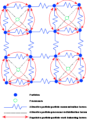
Figure:
Sixteen Data Points Distributed Optimally on Four Processors,
Illustrating the Physical Analogy of Section
11.3
.
We take a simple two-dimensional mesh connection for the particles.
Note that the load-balancing problem becomes that of finding the
equilibrium state of a system of particles with a ``conflict'' between
short-range repulsive (hardcore) and long-range attractive forces.
This scenario is qualitatively similar to classical atomic physics
problems and leads one to expect that the physically based
optimization methods could be effective. This physical analogy is
extended in Section
11.2
where we show that the physical
system exhibits effects that can be associated with temperature and
phase transitions. We also indicate how it needs to be extended for
problems with microscopic structure in their temporal properties.
Next:
11.1.3 Algorithms for Load
Up:
11.1 Load Balancing as
Previous:
11.1.1 Load Balancing a
Guy Robinson
Wed Mar 1 10:19:35 EST 1995
11.1.3 Algorithms for Load Balancing
Next:
11.1.4 Simulated Annealing
Up:
11.1 Load Balancing as
Previous:
11.1.2 The Optimization Problem
This book presents performance evaluation of three load-balancing
algorithms, all of which run in parallel. With a massively parallel machine,
it would not be possible to load-balance the mesh sequentially. This is
because (1) there would be a serious sequential bottleneck,
(2) there would not be enough memory in a host machine to
store the entire distributed mesh, and (3) the large cost incurred in
communicating the entire mesh.
The three methods are:\
-
SA
-Simulated annealing:
We
directly minimize the above cost function by a process analogous to
slow physical cooling.
-
ORB
-Orthogonal recursive bisection:
A simple method which cuts the graph into two by a vertical
cut, then cuts each half into two by a horizontal cut, then cuts each
quarter vertically, and so on. These cuts are usually
motivated by the natural geometrical or physical structure of the
problem [
Baden:87a
], [
Fox:88mm
]. However, they can also be
generated in more abstract fashion directly from a graph [
Fox:88nn
].
-
ERB
-Eigenvector recursive bisection: This method also cuts
the graph in two then each half into two, and so on, but the cutting is done
using an eigenvector of a matrix with the same sparsity structure as the
adjacency matrix of the graph. The method is an approximation to a
computational neural net [
Fox:88e
], [
Williams:91a
].
Guy Robinson
Wed Mar 1 10:19:35 EST 1995
11.1.4 Simulated Annealing
Next:
11.1.5 Recursive Bisection
Up:
11.1 Load Balancing as
Previous:
11.1.3 Algorithms for Load
Simulated annealing
[
Fox:88mm
], [
Hajek:88a
],
[
Kirkpatrick:83a
], [
Otten:89a
] is a very general optimization
method which stochastically simulates the slow cooling of a physical
system. The idea is that there is a cost function
H
(in physical
terms, a Hamiltonian) which associates a cost with a state of the
system, a ``temperature''
T
, and various ways to change the state of
the system. The algorithm works by iteratively proposing changes and
either accepting or rejecting each change. Having proposed a change we
may evaluate the change  in
H
. The proposed change may be
accepted or rejected by the
Metropolis
criterion; if the cost function decreases
in
H
. The proposed change may be
accepted or rejected by the
Metropolis
criterion; if the cost function decreases  the
change is accepted unconditionally; otherwise it is accepted but only
with probability
the
change is accepted unconditionally; otherwise it is accepted but only
with probability  . A crucial requirement for the
proposed changes is
reachability
or
ergodicity
-that there
be a sufficient variety of possible changes that one can always find a
sequence of changes so that any system state may be reached from any
other.
. A crucial requirement for the
proposed changes is
reachability
or
ergodicity
-that there
be a sufficient variety of possible changes that one can always find a
sequence of changes so that any system state may be reached from any
other.
When the temperature is zero, changes are accepted only if
H
decreases, an
algorithm also known as
hill-climbing
, or more generally, the
greedy algorithm
[
Aho:83a
].
The system soon reaches a state in which none
of the proposed changes can decrease the cost function, but this is
usually a poor optimum. In real life, we might be trying to achieve
the highest point of a mountain range by simply walking upwards; we
soon arrive at the peak of a small foothill and can go no further.
On the contrary, if the temperature is very large, all changes are accepted,
and we simply move at random ignoring the cost function. Because of the
reachability property of the set of changes, we explore all states of the
system, including the global optimum.
Simulated annealing consists of running the accept/reject algorithm between
the temperature extremes. We propose many changes, starting at a high
temperature and exploring the state space, and gradually decreasing the
temperature to zero while hopefully settling on the global optimum. It can
be shown that if the temperature decreases sufficiently slowly (the inverse
of the logarithm of the time), then the probability of being in a global
optimum tends to certainty [
Hajek:88a
].
Figure
11.4
shows simulated annealing applied to the load-balancing cost function in one dimension. The graph to be colored is a
periodically connected linear array of 200 nodes, to be colored with four
colors. The initial configuration, at the bottom of the figure, is the left
100 nodes colored white, two domains of 50 each in mid grays, and with no
nodes colored in the darkest gray. We know that the global optimum is 50
nodes of each color, with all the nodes of the same color consecutive.
Iterations run up the figure with the final configurations at the top.
Figure 11.4:
Simulated Annealing of a Ring Graph of Size 200, with the Four
Graph Colors Shown by Gray Shades. The time history of the annealing
runs vertically, with the maximum temperature and the starting
configuration at the bottom, and zero temperature and the final optimum at
the top. The basic move is to change the color of a graph node to a
random color.
At each iteration of the annealing, a random node is chosen, and its color
changed to a random color. This proposed move is accepted if the Metropolis
criterion is accepted. At the end of the annealing, a good balance is
achieved at the top of the figure, with each color having equal numbers
of nodes; but there are 14 places where the color changes (communication
cost = 14), rather than the minimum four.
Heuristics
In choosing the change to be made to the state of the system, there may be
intuitive or heuristic reasons to choose a change which tends to reduce the
cost function. For our example of load balancing, we know that the optimal
coloring of the graph has equal-sized compact ``globules''; if we were to
restrict the new color of a node to the color of one of its two neighbors,
then the boundaries between colors move without creating new domains.
The effect of this algorithm is shown in Figure
11.5
, with the same
number of iterations as Figure
11.4
. The imbalance of 100 white
nodes is quickly removed, but there are only three colors of 67 nodes each in
the (periodically connected) final configuration. The problem is that the
changes do not satisfy reachability; if a color is not present in graph
coloring, then it can never come back.
Figure:
Same as Figure
11.4
, Except the Basic Move Is to
Change the Color of a Graph Node to the Color of One of the Neighbors.
Even if reachability is satisfied, a heuristic may degrade the quality of the
final optimum, because a heuristic is coercing the state toward local minima
in much the same way that a low temperature would. This may reduce the
ability of the annealing algorithm to explore the state space, and cause it to
drop into a local minimum and stay there, resulting in poor performance
overall.
Figure
11.6
shows a solution to this problem. There is a high
probability the new color is one of the neighbors, but also a small
probability of a ``seed'' color, which is a randomly chosen color. Now we see
a much better final configuration, close to the global optimum. The balance
is perfect and there are five separate domains instead of the optimal four.
Figure:
Same as Figure
11.4
, Except the Basic Move Is to
Change the Color of a Graph Node to the Color of One of the Neighbors
with Large Probability, and to a Random Color with Small Probability.
Collisional Simulated Annealing
As presented so far, simulated annealing is a sequential algorithm,
since whenever a move is made an acceptance decision must be made
before another move may be evaluated. A parallel variant, which we
shall call
collisional
simulated annealing,
would be to propose several changes to the state
of the system, evaluate the Metropolis criterion on each
simultaneously, then make those changes which are accepted.
Figure
11.7
shows the results of the same set of changes as
Figure
11.6
, but doing 16 changes simultaneously instead of
sequentially. Now there are eight domains in the final configuration
rather than five. The essential difference from the sequential
algorithm is that  resulting from several simultaneous
changes is not the sum of the
resulting from several simultaneous
changes is not the sum of the  values if the changes are made
in sequence. We tend to get
parallel collisions
,
where there may be two changes, each of which is beneficial,
but which together are detrimental. For example, a married couple
might need to buy a lawnmower;
if either buys it,
the result is beneficial to the couple, but if both simultaneously buy
lawn mowers, the result is detrimental because they only need one.
values if the changes are made
in sequence. We tend to get
parallel collisions
,
where there may be two changes, each of which is beneficial,
but which together are detrimental. For example, a married couple
might need to buy a lawnmower;
if either buys it,
the result is beneficial to the couple, but if both simultaneously buy
lawn mowers, the result is detrimental because they only need one.
Figure:
Same as Figure
11.6
, Except the Optimization Is
Being Carried Out in Parallel by 16 Processors. Note the fuzzy edges of
the domains caused by parallel collisions.
Figure
11.8
shows how parallel collisions can adversely
affect the load-balancing process. At left, two processors share a
small mesh, shown by the two colors, with a sawtooth division between
them. There are seven edges with different colors on each side. In
the middle are shown each processor's separate views of the situation,
and each processor discovers that by changing the color of the teeth of
the sawtooth it can reduce the boundary from 7 to 4. On the right is
shown the result of these simultaneous changes; the boundary has
increased to 15, instead of the 4 that would result if only one
processor went ahead.
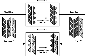
Figure 11.8:
Illustration of a Parallel Collision During Load Balance. Each
processor may take changes which decrease the boundary length, but the
combined changes increase the boundary.
The problem with this parallel variant is, of course, that we are no longer
doing the correct algorithm, since each processor is making changes without
consulting the others. As noted in [
Baiardi:89a
], [
Barajas:87a
],
[
Braschi:90a
], [
Williams:86b
], we have an algorithm which is
highly parallel, but not particularly efficient. We should note that when
the temperature is close to zero, the success rate of changes (ratio of
accepted to proposed changes) falls to zero: Since a parallel collision
depends on two successful changes, the parallel collision rate is proportional
to the square of the low success rate, so that the effects of parallel
collisions must be negligible at low temperatures.
One approach [
Fox:88a
] [
Johnson:86a
] to the parallel
collision problem is
rollback
.
We make the
changes in parallel, as above, then check to see if any parallel
collisions have occurred, and if so, undo enough of the changes so that
there are no collisions. While rollback ensures that the algorithm is
carried out correctly, there may be a great deal of overhead,
especially in a tightly coupled system at high temperature, where each
change may collide with many others, and where most changes will be
accepted. In addition, of course, rollback involves a large software
and memory overhead since each change must be recorded in such a way
that it can be rescinded, and a decision must be reached about which
changes are to be undone.
For some cost functions and sets of changes, it may be possible to divide the
possible changes into classes such that parallel changes within a class do
not collide. An important model in statistical physics is the
Potts
model
[
Wu:82a
], whose cost function is the same as the communication
part of the load-balance cost function. If the underlying graph is a square
lattice, the graph nodes may be divided into ``red'' and ``black'' classes, so
called because the arrangement is like the red and black squares of a
checkerboard
. Then we may change all the red
nodes or all the black nodes in parallel with no collisions.
Some highly efficient parallel simulated annealing algorithms have been
implemented [
Coddington:90a
] for the Potts model
using
clustering.
These methods are based on the locality
of the Potts cost function: the change in cost function from a
change in the color of a graph node depends only on the colors of the
neighboring nodes of the graph. Unfortunately, the balance part of the
cost function interferes with this locality in that widely separated
(in terms of the Hamming distance) changes may collide, so these
methods are not suitable for load balancing.
In this book, we shall use the simple collisional simulated annealing
algorithm, making changes without checking for parallel collisions. Further
work is required to invent and test more sophisticated parallel algorithms
for simulated annealing, which may be able to avoid the degradation of
performance caused by parallel collisions without unacceptable inefficiency
from the parallelism [
Baiardi:89a
].
Clustering
Since the basic change made in the graph-coloring problem is to change the
color of one node, a boundary can move at most one node per iteration. The
boundaries between processors are diffusing toward their optimal
configurations. A better change is to take a connected set of nodes
which are the same color, and change the color of the entire set at once
[
Coddington:90a
]. This is shown in Figure
11.9
where the
cluster is chosen first by picking a random node; we then add nodes
probabilistically to the cluster; in this case, the neighbor is added with
probability 0.8 if it has the same color, and never if it has a different
color. Once a neighbor has failed to be added, the cluster generation
finishes. The coloring of the graph becomes optimal extremely quickly
compared to the single color change method of Figure
11.6
.
Figure:
Same as Figure
11.6
, Except the Basic Move Is to
Change the Color of a Connected Cluster of Nodes.
Figure
11.10
shows the clustered simulated annealing running in
parallel, where 16 clusters are chosen simultaneously. The performance is
degraded, but still better than Figure
11.7
, which is parallel but
with single color changes.
Figure:
Same as Figure
11.7
, Except That the Cluster Method
Is Being Carried Out in Parallel by 16 Processors.
Summary of the Algorithm
The annealing algorithm as presented so far requires that several parameters
be chosen for tuning, which are in
italic font
in the description
below.
First, we pick the initial coloring of the graph so that each graph node takes
a color corresponding to the processor in which it currently resides. We
form a population table, of which each processor has a copy of  , the
number of nodes which have color
q
. We pick a value for
, the
number of nodes which have color
q
. We pick a value for  , the
importance of communication
.
, the
importance of communication
.
We pick a
maximum temperature
and the
number of stages
during
which the temperature is to be reduced to zero. Each stage consists of a
number of changes to the graph coloring which may be accepted or rejected,
with no communication between the processors. At the end of the stage, each
processor has a different idea of the population table, and the colors of
neighboring graph nodes which are in different processors, because each
processor has made changes without knowledge of the others. At the end of
the stage, the processors communicate to update the population tables and
local neighbor information so that each processor has up-to-date information.
Each stage consists of either having a given
number of accepted changes
,
or a
given number of rejected changes
, whichever comes first,
followed by a loosely synchronous communication between processors.
Each trial move within a stage consists of looking for a cluster of uniform
color, choosing a new color for the cluster, evaluating the change in cost
function, and using the Metropolis
criterion to
decide whether to accept it. The cluster is chosen by first picking a
random graph node as a seed, and probabilistically forming a cluster.
Neighboring nodes are added to the cluster with a given
cluster
probability
if they are the same color as the seed and reside in the
same processor.
The proposed new color for the cluster is chosen to be either random with
given
seed probability
, or a random color chosen from the set of
neighbors of the cluster. The Metropolis criterion is then used to decide if
the color change is to be accepted, and if so, the local copy of the
population table is updated.
Next:
11.1.5 Recursive Bisection
Up:
11.1 Load Balancing as
Previous:
11.1.3 Algorithms for Load
Guy Robinson
Wed Mar 1 10:19:35 EST 1995
11.1.5 Recursive Bisection
Next:
11.1.6 Eigenvalue Recursive Bisection
Up:
11.1 Load Balancing as
Previous:
11.1.4 Simulated Annealing
Rather than coloring the graph by direct minimization of the load-balance
cost function, we may do better to reduce the problem to a number of
smaller problems. The idea of recursive bisection
is that it is easier to color a graph with two colors than
many colors. We first split the graph into two halves, minimizing the
communication between the halves. We can then color each half with two
colors, and so on, recursively bisecting each subgraph.
There are two advantages to recursive bisection; first, each subproblem
(coloring a graph with two colors) is easier than the general problem;
second, there is natural parallelism. While the first stage is
splitting a single graph in two, and is thus a sequential problem, there is
two-way parallelism at the second stage, when the two halves are being split,
and four-way parallelism when the four quarters are being split. Thus,
coloring a graph with
P
colors is achieved in a number of stages which is
logarithmic in
P
.
Both of the recursive bisection methods we shall discuss split a graph into
two by associating a scalar quantity,  , with each graph node,
e
, which
we may call a
separator
field. By evaluating the median
S
of the
, with each graph node,
e
, which
we may call a
separator
field. By evaluating the median
S
of the
 , we can color the graph according to whether
  is greater or less
than
S
. The median is chosen as the division so that the number of nodes
in each half is automatically equal; the problem is now reduced to that of
choosing the field,
is greater or less
than
S
. The median is chosen as the division so that the number of nodes
in each half is automatically equal; the problem is now reduced to that of
choosing the field,  , so that the communication is minimized.
Orthogonal Recursive Bisection
A simple and cheap choice [
Fox:88mm
] for the separator field is based on
the position of the finite elements in the mesh. We might let the value
of  be the
x
-coordinate of the center of mass of the element, so that
the mesh is split in two by a median line parallel to the
y
-axis. At the
next stage, we split the submesh by a median line parallel to the
x
-axis,
alternating between
x
and
y
stage by stage, as shown in
Figure
11.11
. Another example is shown in
Figure
12.13
.
be the
x
-coordinate of the center of mass of the element, so that
the mesh is split in two by a median line parallel to the
y
-axis. At the
next stage, we split the submesh by a median line parallel to the
x
-axis,
alternating between
x
and
y
stage by stage, as shown in
Figure
11.11
. Another example is shown in
Figure
12.13
.
Figure 11.11:
Load Balancing by ORB for Four Processors. The elements (left)
are reduced to points at their centers of mass (middle), then split into
two vertically, then each half split into two horizontally. The result
(right) shows the assignment of elements to processors.
Next:
11.1.6 Eigenvalue Recursive Bisection
Up:
11.1 Load Balancing as
Previous:
11.1.4 Simulated Annealing
Guy Robinson
Wed Mar 1 10:19:35 EST 1995
11.1.6 Eigenvalue Recursive Bisection
Next:
11.1.7 Testing Procedure
Up:
11.1 Load Balancing as
Previous:
11.1.5 Recursive Bisection
Better but more expensive methods for splitting a graph are based on
finding a particular eigenvector of a sparse matrix
which has the structure of the adjacency matrix of the graph,
and using this eigenvector as a separator field [
Barnes:82a
],
[
Boppana:87a
], [
Pothen:89a
].
Neural Net Model
For our discussion of eigenvector bisection, we use the concept of a
computational neural net,
based on the model of
Hopfield and Tank [
Fox:88tt
], [
Hopfield:85b
]. When the graph
is to be colored with two colors, these may be conveniently represented
by the two states of a neuron, which we conventionally represent by the
numbers
-1
and
+1
. The Hopfield-Tank neural net finds the minimum
of a ``computational energy,'' which is a negative-definite quadratic
form over a space of variables which may take these values
-1
and
+1
, and consequently is ideally suited to the two-processor load-balance
problem. Rewriting the load balance cost function,

where the  are
``neural firing rates,'' which are continuous variables during the
computation and tend to 1 as the computation progresses. The first
term of this expression is the communication part of the cost function,
the second term ensures equal numbers of the two colors if
are
``neural firing rates,'' which are continuous variables during the
computation and tend to 1 as the computation progresses. The first
term of this expression is the communication part of the cost function,
the second term ensures equal numbers of the two colors if  is
small enough, and the third term is zero when the
is
small enough, and the third term is zero when the  are 1, but
pushes the
are 1, but
pushes the  away from zero during the computation. The latter
is to ensure that
H
is negative-definite, and the large but arbitrary
constant
away from zero during the computation. The latter
is to ensure that
H
is negative-definite, and the large but arbitrary
constant  plays no part in the final computation. The firing rate
or output
plays no part in the final computation. The firing rate
or output  of a neuron is related to its
activity
of a neuron is related to its
activity
 by
a sigmoid function which we may take to be
by
a sigmoid function which we may take to be  . The
constant
. The
constant  adjusts the ``gain'' of the neuron as an amplifier. The
evolution equations to be solved are then:
adjusts the ``gain'' of the neuron as an amplifier. The
evolution equations to be solved are then:

where  is a time constant for the system
and
is a time constant for the system
and  is the degree (number of neighbors) of the graph node
e
.
If the gain is sufficiently low, the stable solution of this set of
equations is that all the
is the degree (number of neighbors) of the graph node
e
.
If the gain is sufficiently low, the stable solution of this set of
equations is that all the  are zero, and as the gain becomes
large, the
are zero, and as the gain becomes
large, the  grow and the
  tend to either
-1
or
+1
. The
neural approach to load balancing thus consists of slowly increasing
the gain from zero while solving this set of coupled nonlinear
differential equations.
tend to either
-1
or
+1
. The
neural approach to load balancing thus consists of slowly increasing
the gain from zero while solving this set of coupled nonlinear
differential equations.
Let us now linearize this set of equations for small values of  , meaning
that we neglect the hyperbolic tangent, because for small
x
,
, meaning
that we neglect the hyperbolic tangent, because for small
x
,  . This linear set of equations may be written in terms of the
vector
u
of all the
. This linear set of equations may be written in terms of the
vector
u
of all the  values and the adjacency matrix
A
of
the graph, whose element
values and the adjacency matrix
A
of
the graph, whose element  is 1 if and only if the distinct graph
nodes
e
and
f
are connected by an edge of the graph. We may write
is 1 if and only if the distinct graph
nodes
e
and
f
are connected by an edge of the graph. We may write

where
D
is a diagonal matrix whose elements are the degrees of the
graph nodes,
I
is the identity matrix, and
E
is the matrix
with 1 in each entry. This linear set of equations may be solved exactly
from a knowledge of the eigenvalues and eigenvectors
of the symmetric matrix
N
. If  is sufficiently large, all
eigenvalues of
N
are positive, and when
is sufficiently large, all
eigenvalues of
N
are positive, and when  is greater than a critical value, the eigenvector of
N
corresponding to its largest eigenvalue grows exponentially. Of
course, when the neuron activities are no longer close to zero, the
growth is no longer exponential, but this initial growth determines the
form of the emerging solution.
is greater than a critical value, the eigenvector of
N
corresponding to its largest eigenvalue grows exponentially. Of
course, when the neuron activities are no longer close to zero, the
growth is no longer exponential, but this initial growth determines the
form of the emerging solution.
If  is sufficiently small, so that balance is strongly enforced, then
the eigenspectrum of
N
is dominated by that of
E
. The highest
eigenvalue of
N
must be chosen from the space of the lowest eigenvalue
of
E
. The lowest eigenvalue of
E
is zero, with eigenspace given
by those vectors with
is sufficiently small, so that balance is strongly enforced, then
the eigenspectrum of
N
is dominated by that of
E
. The highest
eigenvalue of
N
must be chosen from the space of the lowest eigenvalue
of
E
. The lowest eigenvalue of
E
is zero, with eigenspace given
by those vectors with  , which is just the balance condition. We
observe that multiples of the identity matrix make no difference to the
eigenvectors, and conclude that the dominant eigenvector
s
satisfies
, which is just the balance condition. We
observe that multiples of the identity matrix make no difference to the
eigenvectors, and conclude that the dominant eigenvector
s
satisfies
 and
and  , where
 is maximal. The matrix
  is the
Laplacian
matrix
of the graph [
Pothen:89a
], and is positive semi-definite. The lowest
eigenvector of the Laplacian has eigenvalue zero, and is explicitly excluded
by the condition
is the
Laplacian
matrix
of the graph [
Pothen:89a
], and is positive semi-definite. The lowest
eigenvector of the Laplacian has eigenvalue zero, and is explicitly excluded
by the condition  . Thus, it is the second eigenvector which we
use for load balancing.
. Thus, it is the second eigenvector which we
use for load balancing.
In summary, we have set up the load balance problem for two processors as a
neural computation problem, producing a set of nonlinear differential
equations to be solved. Rather than solve these, we have assumed that the
behavior of the final solution is governed by the eigenstate which first
emerges at a critical value of the gain. This eigenstate is the second
eigenvector of the Laplacian matrix of the graph.
If we split a connected graph in two equal pieces while minimizing the
boundary, we expect each half to be a connected subgraph of the original
graph. This is not true in all geometries, but is in ``reasonable
cases.'' This intuition is supported by a theorem of Fiedler [Fiedler:75a;75b]
that when we do the splitting by
the second eigenvector of the Laplacian matrix, at least one-half is
always connected.
To calculate this second eigenstate, we use the Lanczos method
[
Golub:83a
], [
Parlett:80a
],
[
Pothen:89a
]. We can explicitly exclude the eigenvector of value
zero, because the form of this eigenvector is equal entries for each
element of the vector. The accuracy of the Lanczos method increases
quickly with the number of
Lanczos vectors
used. We find that
30 Lanczos vectors are sufficient for splitting a graph of 4000 nodes.
A closely related eigenvector method [
Barnes:82a
], [
Boppana:87a
] is
based on the second highest eigenvector of the adjacency matrix of the graph,
rather than the second lowest eigenvector of the Laplacian matrix. The
advantage of the Laplacian method is in the implementation: The first
eigenvector is known exactly (the vector of all equal elements), so that it
can be explicitly deflated in the Lanczos method.
Figure 11.12 (Color Plate) shows eigenvector recursive bisection in
action. A triangular mesh surrounding a four-element airfoil has already
been split into eight pieces, with the pieces separated by gray lines.
Each of these pieces is being split into two, and the plot shows the
value of the eigenvector used to make the next split, shown by black
lines. The eigenvector values range from large and positive in red
through dark and light blue, green, yellow, and back to red. The eight
eigenvector calculations are independent and are, of course, done in
parallel.
Figure 11.12:
A stage of eigenvalue recursive
bisection. A mesh has already been split into eight pieces, which are
separated by gray lines, and the eigenvector is depicted on each of these.
The next split (into sizteen pieces) is shown by the black lines.
Figure 11.13:
Solution of the Laplace Equation Used to Test Load-Balancing
Methods. The outer boundary has voltage increasing linearly from  to
to  in the vertical direction, the light shade is voltage
1
, and
the dark shade voltage
-1
.
in the vertical direction, the light shade is voltage
1
, and
the dark shade voltage
-1
.
The splitting is constructed by finding a median value for the
eigenvector so that half the triangles have values greater than the
median and half lower. The black line is the division between these.
Next:
11.1.7 Testing Procedure
Up:
11.1 Load Balancing as
Previous:
11.1.5 Recursive Bisection
Guy Robinson
Wed Mar 1 10:19:35 EST 1995
11.1.7 Testing Procedure
Next:
11.1.8 Test Results
Up:
11.1 Load Balancing as
Previous:
11.1.6 Eigenvalue Recursive Bisection
The applications described in Section
11.1.1
have been implemented with
DIME (Distributed Irregular Mesh Environment), described in
Section
10.1
.
We have tested these three load-balancing methods using the application
code ``Laplace'' described in Section
11.1.1
. The problem is
to solve Laplace's equation with Dirichlet boundary conditions, in the domain
shown in Figure
11.13
. The square outer boundary has voltage
linearly increasing vertically from  to
to  , the lightly shaded
S-shaped internal boundary has voltage
+1
, and the dark shaded hook-shaped
internal boundary has voltage
-1
. Contour lines of the solution are also
shown in the figure, with contour interval
, the lightly shaded
S-shaped internal boundary has voltage
+1
, and the dark shaded hook-shaped
internal boundary has voltage
-1
. Contour lines of the solution are also
shown in the figure, with contour interval  .
.
The test begins with a relatively coarse mesh of 280 elements, all residing
in a single processor, with the others having none. The Laplace equation is
solved by Jacobi iteration, the mesh is refined based on the solution
obtained so far, then is balanced by the method under test. This
sequence-solve, refine, balance-is repeated seven times until the final
mesh has 5772 elements. The starting and ending meshes are shown in
Figure
11.14
.
Figure 11.14:
Initial and Final Meshes for the Load-Balancing Test. The
initial mesh with 280 elements is essentially a uniform meshing of the
square, and the final mesh of 5772 elements is dominated by the highly
refined S-shaped region in the center.
The refinement is solution-adaptive, so that the set of elements to be
refined is based on the solution that has been computed so far. The
refinement criterion is the magnitude of the gradient of the solution, so
that the most heavily refined part of the domain is that between the S-shaped
and hook-shaped boundaries where the contour lines are closest together. At
each refinement, the criterion is calculated for each element of the mesh, and
a value is found such that a given proportion of the elements are to be
refined, and those with higher values than this are refined loosely
synchronously. For this test of load balancing, we refined 40% of the
elements of the mesh at each stage.
This choice of refinement criterion is not particularly to improve the
accuracy of the solution, but to test the load-balancing methods as the mesh
distribution changes. The initial mesh is essentially a square covered in
mesh of roughly uniform density, and the final mesh is dominated by the long,
thin S-shaped region between the internal boundaries, so the mesh changes
character from two-dimensional to almost one-dimensional.
We ran this test sequence on 16 nodes of an nCUBE/10 parallel machine, using
ORB and ERB and two runs with SA, the difference being a factor of ten in
cooling rate, and different starting temperatures.
The eigenvalue recursive bisection used the deflated Lanczos method for
diagonalization, with three iterations of 30 Lanczos vectors each to find the
second eigenvector. These numbers were chosen so that more iterations and
Lanczos vectors produced no significant improvement, and fewer degraded
the performance of the algorithm.
The parameters used for the collisional annealing were as follows:\
-
The starting temperature for the run labelled SA1 was 0.2, and for
SA2, 1.0. In the former case, movement of the boundaries is
allowed, but a significant memory of the initial coloring is retained. In
the latter case, large fluctuations are allowed, the system is heated to
randomness, and all memory of the initial configuration is erased.
-
The interface (boundary) importance,
 , was set at 0.1, which is
large enough to make communication important in the cost function, but
small enough that all processors will get their share of elements.
, was set at 0.1, which is
large enough to make communication important in the cost function, but
small enough that all processors will get their share of elements.
-
The curves labelled SA1 correspond to cooling to zero temperature in
500 stages, those labelled SA2 to cooling in 5000 stages.
-
Each stage consisted of finding either one successful change (per
processor) or 200 unsuccessful changes before communicating, and thus getting
the correct global picture.
-
The cluster probability was set to 0.58, giving an average cluster size
of about 22. This is a somewhat arbitrary choice and further work is
required to optimize this.
In Figure
11.15
, we show the divisions between processor domains for
the three methods at the fifth stage of the refinement, with 2393 elements
in the mesh. The figure also shows the divisions for the ORB method at the
fourth stage: Note the unfortunate processor division to the left of the
S-shaped boundary which is absent at the fifth stage.
Figure 11.15:
Processor Divisions Resulting from the Load-Balancing
Algorithms. Top, ORB at the fourth and fifth stages; lower left, ERB at
the fifth stage; lower right, SA2 at the fifth stage.
Next:
11.1.8 Test Results
Up:
11.1 Load Balancing as
Previous:
11.1.6 Eigenvalue Recursive Bisection
Guy Robinson
Wed Mar 1 10:19:35 EST 1995
11.1.8 Test Results
Next:
11.1.9 Conclusions
Up:
11.1 Load Balancing as
Previous:
11.1.7 Testing Procedure
We made several measurements of the running code, which can be
divided into three categories:\
Machine-independent Measurements
These are measurements of the quality of the solution to the
graph-partitioning problem which are independent of the particular
machine on which the code is run.
Let us define
load imbalance
to be the difference between the maximum
and minimum numbers of elements per processor compared to the average number
of elements per processor. More precisely, we should use equations
(i.e., work) per processor as, for instance, with Dirichlet boundary
conditions, the finite element boundary nodes are inactive and
generate no equations [
Chrisochoides:93a
].
The two criteria for measuring communication overhead are the
total
traffic size
, which is the sum over processors of the number of
floating-point numbers sent to other processors per iteration of the Laplace
solver, and the
number of messages
, which is the sum over processors of
the number of messages used to accomplish this communication.
These results are shown in Figure
11.16
. The load imbalance is
significantly poorer for both the SA runs, because the method does not have
the exact balance built in as do the RB methods, but instead exchanges load
imbalance for reducing the communication part of the cost function. The
imbalance for the RB methods comes about from splitting an odd number of
elements, which of course cannot be exactly split in two.
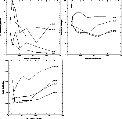
Figure 11.16:
Machine-independent Measures of Load-Balancing Performance.
Left, percentage load imbalance; lower left, total amount of
communication; right, total number of messages.
There is a sudden reduction in total traffic size for the ORB method between
the fourth and fifth stages of refinement. This is caused by the geometry of
the mesh as shown at the top of Figure
11.15
; at the fourth stage
the first vertical bisection is just to the left of the light S-shaped region
creating a large amount of unnecessary communication, and for the fifth and
subsequent stages the cut fortuitously misses the highly refined part of the
mesh.
Machine-dependent Measurements
These are measurements which depend on the particular hardware and
message-passing software on which the code is run. The primary
measurement is, of course, the time it takes the code to run to
completion; this is the sum of startup time, load-balancing time,
and the product of the number of iterations of the inner loop times the
time per iteration. For quasi-static load balancing, we are assuming
that the time spent on the basic problem computation is much longer
than the load-balance time, so parallel computation time is our primary
measurement of load-balancing performance. Rather than use an
arbitrary time unit such as seconds for this measurement, we have
counted this time per iteration as an equivalent number of floating-point
operations (flops). For the nCUBE, this time unit is  for a 64-bit multiply. Thus, we measure
flops per iteration
of the Jacobi solver.
for a 64-bit multiply. Thus, we measure
flops per iteration
of the Jacobi solver.
The secondary measurement is the
communication time
per iteration,
also measured in flops. This is just the local communication in the graph,
and does not include the time for the global combine which is necessary to
decide if the Laplace solver has reached convergence
.
Figure
11.17
shows the timings measured from running the test
sequence on the 16-processor nCUBE. For the largest mesh, the difference in
running time is about 18% between the cheapest load-balancing method (ORB)
and the most expensive (SA2). The ORB method spends up to twice as much time
communicating as the others, which is not surprising, since ORB pays little
attention to the structure of the graph it is splitting, concentrating only
on getting exactly half of the elements on each side of an arbitrary line.
Figure 11.17:
Machine-dependent Measures of Load-Balancing Performance.
Left, running time per Jacobi iteration in units of the time for a
floating-point operation (flop); right, time spent doing local
communication in flops.
The curves on the right of Figure
11.17
show the time spent in local
communication at each stage of the test run. It is encouraging to note the
similarity with the lower left panel of Figure
11.16
, showing that
the time spent communicating is roughly proportional to the total traffic
size, confirming this assumption made in Section
11.1.2
.
Measurements for Dynamic Load Balancing
After refinement of the mesh, one of the load-balancing algorithms is run and
decisions are reached as to which of a processor's elements are to be sent
away, and to which processor they are to be sent. As discussed in
Section
10.1
, a significant fraction of the time taken by the load
balancer is taken in this migration of elements, since not only must the
element and its data be communicated, but space must be allocated in the new
processor and other processors must be informed of the new address of the
element, and so on. Thus, an important measure of the performance of an
algorithm for dynamic (in contrast to quasi-dynamic) load balancing is the
number of
elements migrated
, as a proportion of the total number of
elements.
Figure
11.18
shows the percentage of the elements which migrated
at each stage of the test run. The one which does best here is ORB, because
refinement causes only slight movement of the vertical and horizontal median
lines. The SA runs are different because of the different starting
temperatures: SA1 started at a temperature low enough that the edges of the
domains were just ``warmed up,'' in contrast to SA2 which started at a
temperature high enough to completely forget the initial configuration and,
thus, essentially all the elements are moved. The ERB method causes the
largest amount of element migration, which is because of two reasons. The
first is because some elements are migrated several times because the load
balancing is done in  stages for
P
processors; this is not a
fundamental problem, and arises from the particular implementation of the
method used here. The second reason is that a small change in mesh
refinement may lead to a large change in the second eigenvector; perhaps
a modification of the method could use the distribution of the mesh before
refinement to create an inertial term so that the change in eigenvector as
the mesh is refined could be controlled.
stages for
P
processors; this is not a
fundamental problem, and arises from the particular implementation of the
method used here. The second reason is that a small change in mesh
refinement may lead to a large change in the second eigenvector; perhaps
a modification of the method could use the distribution of the mesh before
refinement to create an inertial term so that the change in eigenvector as
the mesh is refined could be controlled.
Figure 11.18:
Percentage of Elements Migrated During Each Load-Balancing
Stage. The percentage may be greater than 100 because the recursive
bisection methods may cause the same element to be migrated several
times.
The migration time is only part of the time taken to do the load balancing,
the other part being that taken to make the decisions about which element
goes where. The total times for load balancing during the seven stages of
the test run (solving the coloring problem plus the migration time) are shown
in the table below:\
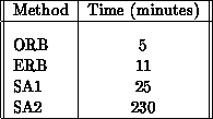
For the test run, the time per iteration was measured in fractions of a
second, and it took few iterations to obtain full
convergence
of the Laplace
equation, so that a high-quality load balance is obviously irrelevant
for this simple case. The point is that the more sophisticated the
algorithm for which the mesh is being used, the greater the time taken
in using the distributed mesh compared to the time taken for the load
balance. For a sufficiently complex application-for example,
unsteady reactive flow simulation-the calculations associated with
each element of the mesh may be enough that a few minutes spent load
balancing is completely negligible, so that the quasi-dynamic
assumption is justified.
Next:
11.1.9 Conclusions
Up:
11.1 Load Balancing as
Previous:
11.1.7 Testing Procedure
Guy Robinson
Wed Mar 1 10:19:35 EST 1995
11.1.9 Conclusions
Next:
Applications and Extensions
Up:
11.1 Load Balancing as
Previous:
11.1.8 Test Results
The Laplace solver that we used for the test run embodies the typical
operation that is done with finite-element meshes. This operation is
matrix-vector multiply. Thus, we are not testing load-balancing
strategies just for a Laplace solver but for a general class of
applications, namely, those which use matrix-vector multiply as the
heart of a scheme which iterates to convergence
on a
fixed mesh, then refines the mesh and repeats the convergence.
The case of the Laplace solver has a high ratio of communication to
calculation, as may be seen from the discussion of Section
11.1.1
, and
thus brings out differences in load-balancing algorithms particularly well.
Each load-balancing algorithm may be measured by three criteria:\
-
the quality of the solution it produces, measured by the time per
iteration in the solver;
-
the time it takes to do the load balancing, measured by the time it
takes to solve the graph-coloring problem and by the number of elements which
must then be migrated; and
-
the portability of the method for different kinds of applications
with different kinds of meshes, and the number of parameters that must be set
to obtain optimal performance from the method.
Orthogonal recursive bisection is certainly cheap, both in terms of the time
it takes to solve the graph-coloring problem and the number of elements which
must be migrated. It is also portable to different applications, the only
required information being the dimensionality of the mesh. And it is easy to
program. Our tests indicate, however, that more expensive methods can
improve performance by over 20%. Because ORB pays no attention to the
connectivity of the element graph, one suspects that as the geometry of the
underlying domain and solution becomes more complex, this gap will widen.
Simulated annealing is actually a family of methods for solving optimization
problems. Even when run sequentially, care must be taken in choosing the
correct set of changes that may be made to the state space, and in choosing a
temperature schedule to ensure a good optimum. We have tried a ``brute force''
parallelization of simulated annealing, essentially ignoring the parallelism.
For sufficiently slow cooling, this method produces the best solution to the
load-balancing problem when measured either against the load-balance cost
function, or by timings on a real parallel computer. Unfortunately, it takes
a long time to produce this high-quality solution, perhaps because some of
the numerous input parameters are not set optimally. A more sensitive
treatment is probably required to reduce or eliminate parallel
collisions [
Baiardi:89a
]. Clearly, further work is required to
make SA a portable and efficient parallel load balancer for parallel
finite-element meshes. True portability may be difficult to achieve
for SA, because the problem being solved is graph coloring, and graphs
are extremely diverse; perhaps something approaching an expert
system may be required to decide the optimal annealing strategy for a
particular graph.
Eigenvalue recursive bisection
seems to be a good compromise between the other methods,
providing a solution of quality near that of SA at a price little more
than that of ORB. There are few parameters to be set, which are
concerned with the Lanczos algorithm for finding the second
eigenvector. Mathematical analysis of the ERB method takes place in
the familiar territory of linear algebra, in contrast to analysis of SA
in the jungles of nonequilibrium thermodynamics. A major point in
favor of ERB for balancing finite-element meshes is that the software
for load balancing with ERB is shared to a large extent with the body
of finite-element software: The heart of the
eigenvector
calculation is a
matrix-vector multiply, which has already been efficiently coded
elsewhere in the finite-element library. Recursive spectral bisection
[
Barnard:93a
] has been developed as a production load balancer and
very successfully applied to a variety of finite-element problems.
The C P research described in this section has been continued by
Mansour in Fox's new group at Syracuse [Mansour:91a;92a-e].
P research described in this section has been continued by
Mansour in Fox's new group at Syracuse [Mansour:91a;92a-e].
He has
considered simulating annealing, genetic algorithms, neural
networks,
and spectral bisection producing in
each parallel implementation. Further, he introduced a
multiscale
or graph contraction approach where large
problems to be decomposed are not directly tackled but are first
``clumped'' or contracted to a smaller problem [
Mansour:93b
],
[
Ponnusamy:93a
]. The latter can be decomposed using the basic
techniques discussed above and this solution of the small problem used
to initialize a fast refinement algorithm for the original large
problem. This strategy has an identical philosophy to the multigrid
approach (Section
9.7
) for partial differential equations. We
are currently collaborating with Saltz in integrating these data
decomposers into the high-level data-parallel languages reviewed in
Section
13.1
.
Next:
Applications and Extensions
Up:
11.1 Load Balancing as
Previous:
11.1.8 Test Results
Guy Robinson
Wed Mar 1 10:19:35 EST 1995
Applications and Extensions of the Physical Analogy
Next:
11.3 Physical Optimization
Up:
11 Load Balancing and
Previous:
11.1.9 Conclusions
In [Fox:86a;92c;92h;93a],
we point out some interesting features of the physical
analogy and energy function introduced in Section
11.1.4
.
Suppose that we are using the simulating annealing method of
Section
11.1.4
on a dynamically varying system. Assume that
this annealing algorithm is running in parallel in the same machine on
which the problem executes. Suppose that we use a (reasonably)
optimal annealing strategy. Even in this case, the ``heatbath''
formed by load balancer
and operating system can
only ``cool'' the problem to a minimum temperature  . At this
temperature, any further gains from improved decomposition by lowering
the temperature will be outweighed by time taken to perform the
annealing. This
temperature
. At this
temperature, any further gains from improved decomposition by lowering
the temperature will be outweighed by time taken to perform the
annealing. This
temperature
 is independent of
performance of computer; it is a property of the system being
simulated. Thus, we can consider this temperature
is independent of
performance of computer; it is a property of the system being
simulated. Thus, we can consider this temperature  as a new
property of a dynamical complex system.
High
values of
as a new
property of a dynamical complex system.
High
values of  imply that the system is rapidly varying; low values
that it is slowly varying.
imply that the system is rapidly varying; low values
that it is slowly varying.
Now we want to show that decompositions can lead to phase
transitions
between different states of the
physical system defined by analogy of Section
11.1.2
. In
the language of Chapter
3
, we can say that the complex
system representing this problem exhibits a phase transition. We
illustrate this with a trivial particle dynamics
problem shown in Figure
11.19
. Typically, we use on
such problems the domain decomposition of Figure
11.19
(a),
where each node of the parallel machine contains a single connected
region (compare Section
12.4
). Alternatively, we can use the
scattered
decomposition-described for
matrices in Section
8.1
and illustrated in
Figure
11.19
(b). One assigns to each processor several small
regions of the space scattered uniformly throughout the domain. Each
processor gets ``a piece of the action'' and shares those parts of the
domain where the particle density and hence computational work is
either large or small. This was explored for partial differential
equations in [
Morison:86a
]. The scattered decomposition is a
local minimum-there is an optimal size for the scattered blocks of
space assigned to each processor. Both in this example and generally,
the scattered decomposition is not as good as domain decomposition.
This is shown in Figure
11.19
(c), which sketches the energy
H
as a function of the chosen decomposition. Now, suppose that the
particles move in time from
t
to  as shown in
Figure
11.19
(d). The scattered decomposition minimum is
unchanged
, but as shown in Figure
11.19
(c),(d) the domain
decomposition minimum moves with time.
as shown in
Figure
11.19
(d). The scattered decomposition minimum is
unchanged
, but as shown in Figure
11.19
(c),(d) the domain
decomposition minimum moves with time.
Figure 11.19:
Particle Dynamics Problem on a Four-node System with Two
Decompositions (a) Domain, Time
t
, (b) Scattered Times
t
and
 , (c) Instantaneous Energies, (d) Domain Decomposition
Changing from Time
t
to
, (c) Instantaneous Energies, (d) Domain Decomposition
Changing from Time
t
to 
Now, one would often be interested not in the instantaneous energy
H
, but rather in the average

For this new objective function  , the scattered
decomposition can be the global minimum as illustrated in
Figure
11.20
. The domain decomposition is smeared with time
and so its minimum is raised in value; the value of
H
at the
scattered decomposition minimum is unchanged. We can study
, the scattered
decomposition can be the global minimum as illustrated in
Figure
11.20
. The domain decomposition is smeared with time
and so its minimum is raised in value; the value of
H
at the
scattered decomposition minimum is unchanged. We can study  as a function of
  , and the hardware ratio
  used in Equation
3.10
. As
used in Equation
3.10
. As  increases or
  decreases, we move from the situation of
Figure
11.19
(c) to that of Figure
11.20
. In
physics language,
decreases, we move from the situation of
Figure
11.19
(c) to that of Figure
11.20
. In
physics language,  and
and  are order parameters which
control the phase transition between the two states
scattered
and
domain
. Rapidly varying systems (high
are order parameters which
control the phase transition between the two states
scattered
and
domain
. Rapidly varying systems (high  ), rather than those with
lower
), rather than those with
lower  , are more likely to see the transition as
  increases.
This agrees with physical intuition, as we now describe. When
increases.
This agrees with physical intuition, as we now describe. When  is
small (slowly varying system), domain decomposition is the global
minimum and this switches to a scattered decomposition as
is
small (slowly varying system), domain decomposition is the global
minimum and this switches to a scattered decomposition as  increases. In Figure
11.19
(a),(b), we can associate with each
particle in the simulation a spin value which indicates the label of
the processor to which it is assigned. Then we see the direct analogy
to physical spin systems. At high temperatures, we have spin waves
(scattered decomposition); at low temperatures, (magnetic) domains
(domain decomposition).
increases. In Figure
11.19
(a),(b), we can associate with each
particle in the simulation a spin value which indicates the label of
the processor to which it is assigned. Then we see the direct analogy
to physical spin systems. At high temperatures, we have spin waves
(scattered decomposition); at low temperatures, (magnetic) domains
(domain decomposition).
Figure:
The Average Energy  of Equation
11.13
of Equation
11.13
We end by noting that in the analogy there is a class of problems which
we call
microscopically dynamic
. These are explored in
[
Fox:88f
], [Fox:88kk;88uu].
In this problem class, the fundamental entities (particles in above
analogy) move between nodes of parallel machine on a microscopic time
scale. The previous discussion had only considered the
adiabatic
loosely synchronous problems where one can assume that the
data elements (particles in the analogy) can be treated as fixed in a
particular processor at each time instant. We will not give a general
discussion here, but rather just illustrate the ideas with one
example-the global sum calculation written in Fortran as
DO l I=l, LIMIT1
A(I)=0
DO 1 J=l, LIMIT2
1 A(I)=A(I) + B(I,J)
This is illustrated in Figure 11.21 (Color Plate) for the case
LIMIT1=4
decomposed onto a four-node machine. The value of
LIMIT1
is
important for performance considerations but irrelevant for the discussion
here. The optimal scheduling of communication and calculation is tricky
and is discussed as the
fold
algorithm in [
Fox:88a
]. The
four tasks of calculating the four
A(I)
cannot be viewed as
particles as they move from node to node and we cannot represent this
movement in the formalism used up to now. Rather, we now represent the
tasks by ``space-time'' strings or world lines and one replaces
Equation
11.9
by a Hamiltonian which describes interacting
strings rather than interacting particles. This can be applied to
event-driven simulations, message routing, and other microscopically
dynamic problems. The strings need to be draped over the space-time
grid formed by the complex computer as it evolves in time.
Figure 11.21 (Color Plate) shows this compact ``draping'' for the fold
algorithm.
Figure 11.21:
The Fold Algorithm. Four global sums
interleaved optimally on four processors.
We have successfully applied similar ideas to multivehicle and multiarm
robot path planning and routing problems [
Chiu:88f
], [Fox:90e;90k;92c],
[
Gandhi:90a
].
Comparison of the vehicle navigation in Figure 11.22 (Color Plate) with the
computational routing problem in Figure 11.21 (Color Plate) illustrates the
analogy.
Figure 11.22:
Two- and four-vechcle navigation
problems. in each case, vehicles have been given initial and final target
positions. The black squares are impassable and define a narrow pass.
Physical optimisation methods[Fox:88ii;90e] were used to find solutions.
Next:
11.3 Physical Optimization
Up:
11 Load Balancing and
Previous:
11.1.9 Conclusions
Guy Robinson
Wed Mar 1 10:19:35 EST 1995
11.3 Physical Optimization
Next:
An Improved Method
Up:
11 Load Balancing and
Previous:
Applications and Extensions
C P maintained a significant activity in optimization.
There were several reasons for this, one of which
was, of course, natural curiosity. Another was the importance of load
balancing and data decomposition which is, as discussed previously in
this chapter, ``just'' an optimization problem. Again, we already
mentioned in Section
6.1
our interest in neural
networks
as a naturally parallel approach to
artificial intelligence. Section
9.9
and Section
11.1
have
shown how neural networks can be used in a range of optimization
problems. Load balancing has the important (optimization)
characteristic of NP completeness, which implies that it would take an
exponential time to solve completely. Thus, we studied the travelling
salesman problem (TSP) which is well known to be NP-complete and
formally equivalent to other problems with this property. One
important contribution of C
P maintained a significant activity in optimization.
There were several reasons for this, one of which
was, of course, natural curiosity. Another was the importance of load
balancing and data decomposition which is, as discussed previously in
this chapter, ``just'' an optimization problem. Again, we already
mentioned in Section
6.1
our interest in neural
networks
as a naturally parallel approach to
artificial intelligence. Section
9.9
and Section
11.1
have
shown how neural networks can be used in a range of optimization
problems. Load balancing has the important (optimization)
characteristic of NP completeness, which implies that it would take an
exponential time to solve completely. Thus, we studied the travelling
salesman problem (TSP) which is well known to be NP-complete and
formally equivalent to other problems with this property. One
important contribution of C P was the work of Simic
[Simic:90a;91a]. [
Simic:91a
]
P was the work of Simic
[Simic:90a;91a]. [
Simic:91a
]
Simic derived the relationship between the neural network
[
Hopfield:86a
] and elastic net [Durbin:87a;89a],
[Rose:90f;91a;93a],
[
Yuille:90a
]
approaches to the TSP. This work has been extensively reviewed
[Fox:91j;92c;92h;92i]
and we will not go into the details
here. A key concept is that of
physical optimization
which
implies the use of a physics approach of minimizing the energy, that
is, finding the ground state of a complex system
set up as a physical analogy to the optimization problem. This idea is
illustrated clearly by the discussion in Section
11.1.3
and
Section
11.2
. One can understand some reasons why a physics
analogy could be useful from two possible plots of the objective
function to be minimized, against the possible configurations, that is,
against the values of parameters to be determined. Physical systems
tend to look like Figure
11.1
(a), where correlated (i.e.,
local) minima are ``near'' global minima. We usually do not get the
very irregular landscape shown in Figure
11.1
(b). In fact,
we do find the latter case with the so-called random field Ising model,
and here conventional physics methods perform poorly
[
Marinari:92a
], [
Guagnelli:92a
]. Ken Rose showed how these
ideas could be generalized to a wide class of optimization problems as
a concept called
deterministic annealing
[
Rose:90f
], [
Stolorz:92a
]. Annealing is
illustrated in Figure 11.23 (Color Plate). One uses temperature to
smooth out the objective function (energy function) so that at high
temperature one can find the (smeared) global minimum without getting
trapped in spurious local minima. Temperature is decreased skillfully
initializing the search at Temperature  by the solution at the
previous higher temperature
by the solution at the
previous higher temperature  . This annealing can be applied
either statistically [
Kirkpatrick:83a
] as in Sections
11.1
and
11.3
or with a deterministic iteration. Neural and
elastic networks can be viewed as examples of deterministic annealing.
Rose generalized these ideas to clustering [Rose:90a;90c;91a;93a];
. This annealing can be applied
either statistically [
Kirkpatrick:83a
] as in Sections
11.1
and
11.3
or with a deterministic iteration. Neural and
elastic networks can be viewed as examples of deterministic annealing.
Rose generalized these ideas to clustering [Rose:90a;90c;91a;93a];
vector quantization used in coding [
Miller:92b
],
[
Rose:92a
]; tracking
[Rose:89b;90b]; and electronic packing [
Rose:92b
].
Deterministic annealing ;has also been used for robot path planning
with many degrees of freedom [
Fox:90k
], [
Gandhi:90b
] (see
also Figure 11.22 (Color Plate)), character recognition
[
Hinton:92a
], scheduling problems
[Gislen:89a;91a], [
Hertz:92a
],
[
Johnston:92a
], and quadratic assignment
[
Simic:91a
].
Figure 11.23:
Annealing tracks global minima by
initializing search at one temperature by minima found at other temperatures .
Neural networks
have been shown to perform poorly
in practice on the TSP [
Wilson:88a
], but we found them excellent
for the formally equivalent load-balancing problem in
Section
11.1
. This is now understood from the fact that the
simple neural networks
used in the TSP
[
Hopfield:86a
] used many redundant neural variables, and the
difficulties reported in [
Wilson:88a
] can be traced to the role of
the constraints that remove redundant variables. The neural network
approach summarized in Section
11.1.6
uses a parameterization that
has no redundancy and so it is not surprising that it works well. The
elastic network can be viewed as a neural network with some constraints
satisfied exactly [
Simic:90a
]. This can also be understood by
generalizing the conventional binary neurons to multistate or Potts
variables
[Peterson:89b;90a;93a].
Moscato developed several novel ways of combining simulated annealing
with genetic algorithms [Moscato:89a;89c;89d;89e]
and
showed the power and flexibility of these methods.
Next:
An Improved Method
Up:
11 Load Balancing and
Previous:
Applications and Extensions
Guy Robinson
Wed Mar 1 10:19:35 EST 1995
An Improved Method for the
Travelling Salesman Problem
Next:
11.4.1 Background on Local
Up:
11 Load Balancing and
Previous:
11.3 Physical Optimization
The Travelling Salesman Problem (TSP) is probably the most well-known
member of the wider field of
combinatorial
optimization
(CO) problems. These are difficult
optimization problems where the set of feasible solutions (trial
solutions which satisfy the constraints of the problem but are not
necessarily optimal) is a finite, though usually very large set. The
number of feasible solutions grows as some combinatoric factor such as
 , where
N
characterizes the size of the problem. We have already
commented on the use of neural networks for the TSP in the previous
section. Here we show how to combine problem-specific heuristics with
simulated annealing, a physical optimization
method.
, where
N
characterizes the size of the problem. We have already
commented on the use of neural networks for the TSP in the previous
section. Here we show how to combine problem-specific heuristics with
simulated annealing, a physical optimization
method.
It has often been the case that progress on the TSP has led to progress
on many CO problems and more general optimization problems. In this
way, the TSP is a playground for the study of CO problems. Though the
present work concentrates on the TSP, a number of our ideas are general
and apply to all optimization problems.
The most significant issues occur as one tries to find extremely good
or exact solutions to the TSP. Many algorithms exist which are fast
and find feasible solutions which are within a few percent of the
optimum length. Here, we present algorithms which will usually find
exact solutions to substantial instances of the TSP. We are limited by
space considerations to a brief presentation of the method-more
details may be found in [
Martin:91a
].
In a general instance of the TSP one is given
N
``cities'' and a
matrix  giving the distance or cost function for going from
city
i
to
j
. Without loss of generality, the distances can be
assumed to be positive. A ``tour'' consists of a list of
N
cities,
giving the distance or cost function for going from
city
i
to
j
. Without loss of generality, the distances can be
assumed to be positive. A ``tour'' consists of a list of
N
cities,
 , where each city appears once and only once. In the TSP, the
problem is to find the tour with the minimum ``length,'' where length
is defined to be the sum of the lengths along each step of the tour,
, where each city appears once and only once. In the TSP, the
problem is to find the tour with the minimum ``length,'' where length
is defined to be the sum of the lengths along each step of the tour,
and  is
identified with
is
identified with  to make it periodic.
Most common instances of the TSP have a symmetric distance matrix; we
will hereafter focus on this case. All CO problems can be formulated
as optimizing an objective function (e.g., the length) subject to
constraints (e.g., legal tours).
Next:
11.4.1 Background on Local
Up:
11 Load Balancing and
Previous:
11.3 Physical Optimization
Guy Robinson
Wed Mar 1 10:19:35 EST 1995
11.4.1 Background on Local Search Heuristics
Next:
Background on Markov
Up:
An Improved Method
Previous:
An Improved Method
In a local search method, one first defines a neighborhood topology on the set
of all tours. For instance, one might define the neighborhood of a tour
 to be all those tours which can be obtained by changing at most
k
edges of
to be all those tours which can be obtained by changing at most
k
edges of  . A tour is said to be
locally opt
if no tour in its
neighborhood is shorter than it. One can search for locally opt tours by
starting with a random tour
. A tour is said to be
locally opt
if no tour in its
neighborhood is shorter than it. One can search for locally opt tours by
starting with a random tour  and performing
k
-changes on it as long
as the tour length decreases. In this way, one constructs a sequence of
tours
and performing
k
-changes on it as long
as the tour length decreases. In this way, one constructs a sequence of
tours  ,
,  ,
,  . Eventually the process stops and one has
reached a local opt tour. Lin [
Lin:65a
] studied the case of
k=2
and
k=3
, and showed that one could get quite good tours quickly.
Furthermore, since in general there are quite a few locally opt tours, in
order to find the globally optimal tour, he suggested repeating this process
from random starts many times until one was confident all the locally opt
tours had been found. Unfortunately, the number of local opt tours rises
exponentially with
N
, the number of cities. Thus in general, it is more
efficient to use a more sophisticated local opt (say higher
k
) than to try
to repeat the search from random starts many times. The current
state-of-the-art optimization heuristic is an algorithm due to Lin and
Kernighan [
Lin:73a
]. It is a variable depth
k
-neighborhood search,
and it is the benchmark against which all heuristics are tested. Since it is
significantly better than three-opt, for any instance of the TSP, there are
many fewer
L
-
K
-opt tours than there are three-opt tours. This
postpones the problem of doing exponentially many random starts until one
reaches
N
on the order of a few hundred. For still larger
N
, the number
of
L
-
K
-opt tours itself gets unmanageable. Given that one really does
want to tackle these larger problems, there are two natural ways to go.
First, one can try to extend the neighborhood which
L
-
K
considers, just
as
L
-
K
extended the neighborhood of three-changes. Second, one expects
that instead of sampling the local opt tours in a random way as is done by
applying the local searches from random starts many times, it might be
possible to obtain local opt tours in a more efficient way, say via a
sampling with a bias in favor of the shorter tours. We will see that this
gives rise to an algorithm which indeed enables one to solve much larger
instances.
. Eventually the process stops and one has
reached a local opt tour. Lin [
Lin:65a
] studied the case of
k=2
and
k=3
, and showed that one could get quite good tours quickly.
Furthermore, since in general there are quite a few locally opt tours, in
order to find the globally optimal tour, he suggested repeating this process
from random starts many times until one was confident all the locally opt
tours had been found. Unfortunately, the number of local opt tours rises
exponentially with
N
, the number of cities. Thus in general, it is more
efficient to use a more sophisticated local opt (say higher
k
) than to try
to repeat the search from random starts many times. The current
state-of-the-art optimization heuristic is an algorithm due to Lin and
Kernighan [
Lin:73a
]. It is a variable depth
k
-neighborhood search,
and it is the benchmark against which all heuristics are tested. Since it is
significantly better than three-opt, for any instance of the TSP, there are
many fewer
L
-
K
-opt tours than there are three-opt tours. This
postpones the problem of doing exponentially many random starts until one
reaches
N
on the order of a few hundred. For still larger
N
, the number
of
L
-
K
-opt tours itself gets unmanageable. Given that one really does
want to tackle these larger problems, there are two natural ways to go.
First, one can try to extend the neighborhood which
L
-
K
considers, just
as
L
-
K
extended the neighborhood of three-changes. Second, one expects
that instead of sampling the local opt tours in a random way as is done by
applying the local searches from random starts many times, it might be
possible to obtain local opt tours in a more efficient way, say via a
sampling with a bias in favor of the shorter tours. We will see that this
gives rise to an algorithm which indeed enables one to solve much larger
instances.
Next:
Background on Markov
Up:
An Improved Method
Previous:
An Improved Method
Guy Robinson
Wed Mar 1 10:19:35 EST 1995
Background on Markov Chains and SimulatedAnnealing
Next:
11.4.3 The New Algorithm-Large-Step
Up:
An Improved Method
Previous:
11.4.1 Background on Local
Given that any local search method will stop in one of the many local opt
solutions, it may be useful to find a way for the iteration to escape by
temporarily allowing the tour length to increase. This leads to the
popular method of ``simulated annealing''
[
Kirkpatrick:83a
].
One starts by constructing a sequence of tours  ,
,  , and so
on. At each step of this chain, one does a
k
-change (moves to a
neighboring tour). If this decreases the tour length, the change is
accepted; if the tour length increases, the change is rejected with
some probability, in which case one simply keeps the old tour at that
step. Such a stochastic construction of a sequence of
T
s is called a
Markov chain
. It can be viewed as a rather
straightforward extension of the above local search to include
``noisiness'' in the search for shorter tours. Because increases in
the tour length are possible, this chain never reaches a fixed point.
For many such Markov chains, it is possible to show that given enough
time, the chain will visit every possible tour
T
, and that for very
long chains, the
T
s appear with a calculable probability
distribution. Such Markov chains are closely inspired by physical
models where the chain construction procedure is called a Monte
Carlo.
The stochastic accept/reject part is
supposed to simulate a random fluctuation due to temperature effects,
and the temperature is a parameter which measures the bias towards
short tours. If one wants to get to the globally optimal tour, one has
to move the temperature down towards zero, corresponding to a strong
bias in favor of short tours. Thus, one makes the temperature vary
with time, and the way this is done is called the annealing schedule,
and the result is simulated annealing.
, and so
on. At each step of this chain, one does a
k
-change (moves to a
neighboring tour). If this decreases the tour length, the change is
accepted; if the tour length increases, the change is rejected with
some probability, in which case one simply keeps the old tour at that
step. Such a stochastic construction of a sequence of
T
s is called a
Markov chain
. It can be viewed as a rather
straightforward extension of the above local search to include
``noisiness'' in the search for shorter tours. Because increases in
the tour length are possible, this chain never reaches a fixed point.
For many such Markov chains, it is possible to show that given enough
time, the chain will visit every possible tour
T
, and that for very
long chains, the
T
s appear with a calculable probability
distribution. Such Markov chains are closely inspired by physical
models where the chain construction procedure is called a Monte
Carlo.
The stochastic accept/reject part is
supposed to simulate a random fluctuation due to temperature effects,
and the temperature is a parameter which measures the bias towards
short tours. If one wants to get to the globally optimal tour, one has
to move the temperature down towards zero, corresponding to a strong
bias in favor of short tours. Thus, one makes the temperature vary
with time, and the way this is done is called the annealing schedule,
and the result is simulated annealing.
If the temperature is taken to zero too fast, the effect is essentially
the same as setting the temperature to zero exactly, and then the chain
just traps at a local opt tour forever. There are theoretical results
on how slowly the annealing has to be done to be sure that one reaches
the globally optimum solution, but in practice the running times are
astronomical. Nevertheless, simulated annealing is a standard and
widely used approach for many minimization problems. For the TSP, it
is significantly slower than Lin-Kernighan,
but it has the advantage that one can run for long times and
slowly improve the quality of the solutions. See, for instance, the
studies Johnson et al. [
Johnson:91a
] have done. The advantage is
due to the improved sampling of the short length tours: Simulated
annealing is able to ignore the tours which are not near the minimum
length. An intuitive way to think about it is that for a long run,
simulated annealing is able to try to improve an already very good
tour, one which probably has many links in common with the exact
optimum. The standard Lin-Kernighan algorithm, by contrast,
continually restarts from scratch, throwing away possibly useful
information.
Next:
11.4.3 The New Algorithm-Large-Step
Up:
An Improved Method
Previous:
11.4.1 Background on Local
Guy Robinson
Wed Mar 1 10:19:35 EST 1995
11.4.3 The New Algorithm-Large-Step Markov Chains
Next:
11.4.4 Results
Up:
An Improved Method
Previous:
Background on Markov
Simulated annealing
does not take
advantage of the local opt heuristics. This means that instead of
sampling local opt tours as does
L
-
K
repeated from random starts,
the chain samples all tours. It would be a great advantage to be able
to restrict the sampling of a Markov chain to the local opt tours
only. Then the bias which the Markov chain provides would enable one
to sample the shortest local opt tours more efficiently than local opt
repeated from random starts. This is what our new algorithm does.
To do this, one has to find a way to go from one local opt tour,  , to
another,
, to
another,  , and this is the heart of our procedure. We propose to do
a change on
, and this is the heart of our procedure. We propose to do
a change on  , which we call a ``kick.'' This can be a random
p
-change,
for instance, but we will choose something smarter than that. Follow this
kick by the local opt tour improvement heuristic until reaching a new local
opt tour
, which we call a ``kick.'' This can be a random
p
-change,
for instance, but we will choose something smarter than that. Follow this
kick by the local opt tour improvement heuristic until reaching a new local
opt tour  . Then accept or reject
  depending on the
increase or decrease in tour length compared to
depending on the
increase or decrease in tour length compared to  . This is illustrated
in Figure
11.24
. Since there are many changes in going from
. This is illustrated
in Figure
11.24
. Since there are many changes in going from  to
to  , we call this method a ``Large-Step Markov Chain.'' It can
also be called ``Iterated Local Opt,'' but it should be realized that it is
precisely finding a way to iterate which is the difficulty! The algorithm is
far better than the small-step Markov chain methods (conventional simulated
annealing) because the accept/reject procedure is not implemented on the
intermediate tours which are almost always of longer length. Instead, the
accept/reject does not happen until the system has returned to a local
minimum. The method directly steps from one local minimum to another. It is
thus much easier to escape from local minima.
, we call this method a ``Large-Step Markov Chain.'' It can
also be called ``Iterated Local Opt,'' but it should be realized that it is
precisely finding a way to iterate which is the difficulty! The algorithm is
far better than the small-step Markov chain methods (conventional simulated
annealing) because the accept/reject procedure is not implemented on the
intermediate tours which are almost always of longer length. Instead, the
accept/reject does not happen until the system has returned to a local
minimum. The method directly steps from one local minimum to another. It is
thus much easier to escape from local minima.
Figure 11.24:
Schematic Representation of the Objective Function and of the
Tour Modification Procedure Used in the Large-step Markov Chain
At this point, let us mention that this method is no longer a true
simulated annealing algorithm. That is, the algorithm does NOT
correspond to the simulation of any physical system undergoing
annealing. The reason is that a certain symmetry property, termed
``detailed balance''
in the physics community,
is not satisfied by the large-step algorithm. [
Martin:91a
] says a
bit more about this. One consequence of this is that the parameter
``temperature'' which one anneals with no longer plays the role of a
true, physical temperature-instead it is merely a parameter which
controls the bias towards the optimum. The lack of a physical analogy
may be the reason that this algorithm has not been tried before, even
though much more exotic algorithms (such as appealing to quantum
mechanical analogies!) have been proposed.
We have found that in practice, this methodology provides an efficient
sampling of the local opt tours. There are a number of criteria which need
to be met for the biased sampling of the Markov chain to be more efficient
than plain random sampling. These conditions are satisfied for the TSP, and
more generally whenever local search heuristics are useful. Let us stress
before proceeding to specifics that this large-step Markov chain approach is
extremely general, being applicable to any optimization
problem where one has local search heuristics. It enables one to get a
performance which is at least as good as local search, with substantial
improvements over that if the sampling can be biased effectively.
Finally, although the method is general, it can be adapted to match the
problem of interest through the choice of the kick. We will now
discuss how to choose the kick for the TSP.
Consider, for instance, the case where the local search is three-opt. If we
used a kick consisting of a three-change, the three-opt would very often
simply bring us back to the previous tour with no gain. Thus, it is probably
a good idea to go to a four-change for the kick when the local search is
three-opt. For more general local search algorithms, a good choice for the
kick would be a
k
-change which does not occur in the local search.
Surprisingly, it turns out that two-opt, three-opt, and especially
L
-
K
are structured so that there is one kick choice which is natural for all of
them. To see this, it is useful to go back to the paper by Lin and
Kernighan. In that paper, they define ``sequential'' changes and they also show
that if the tour is to be improved, one can force all the partial gains during
the
k
-change to be positive. A consequence of this is that the
checkout time for sequential
k
-changes can be completed in  steps.
It is easy to see that all two and three changes are sequential, and that the
first nonsequential change occurs at
k=4
(Figure 2 of their paper). We
call this graph a ``double-bridge'' change because of what it does to the tour.
It can be constructed by first doing a two-change which disconnects the tour;
the second two-change must then reconnect the two parts, thereby creating a
bridge. Note that both of the two-changes are bridges in their own way, and
that the double-bridge change is the only nonsequential four-change which
cannot be obtained by composing changes which are both sequential and leave
the tour connected. If we included this double-bridge change in the
definition of the neighborhood for a local search, checkout time would
require
steps.
It is easy to see that all two and three changes are sequential, and that the
first nonsequential change occurs at
k=4
(Figure 2 of their paper). We
call this graph a ``double-bridge'' change because of what it does to the tour.
It can be constructed by first doing a two-change which disconnects the tour;
the second two-change must then reconnect the two parts, thereby creating a
bridge. Note that both of the two-changes are bridges in their own way, and
that the double-bridge change is the only nonsequential four-change which
cannot be obtained by composing changes which are both sequential and leave
the tour connected. If we included this double-bridge change in the
definition of the neighborhood for a local search, checkout time would
require  steps (a factor
N
for each bridge essentially). Rather
than doing this change as part of the local search, we include such changes
stochastically as our kick. The double-bridge kick is the most natural
choice for any local search method which considers only sequential changes.
Because
L
-
K
does so many changes for
k
greater than three, but misses
double-bridges, one can expect that most of what remains in excess length
using
L
-
K
might be removed with our extension. The results below
indicate that this is the case.
steps (a factor
N
for each bridge essentially). Rather
than doing this change as part of the local search, we include such changes
stochastically as our kick. The double-bridge kick is the most natural
choice for any local search method which considers only sequential changes.
Because
L
-
K
does so many changes for
k
greater than three, but misses
double-bridges, one can expect that most of what remains in excess length
using
L
-
K
might be removed with our extension. The results below
indicate that this is the case.
Next:
11.4.4 Results
Up:
An Improved Method
Previous:
Background on Markov
Guy Robinson
Wed Mar 1 10:19:35 EST 1995
11.4.4 Results
Next:
Irregular Loosely Synchronous
Up:
An Improved Method
Previous:
11.4.3 The New Algorithm-Large-Step
At first we implemented the Large-Step Markov Chain for the three-opt local
search. We checked that we could solve to optimality problems of sizes up to
200 by comparing with a branch and bound program. For
N=100
, the
optimum was found in a few minutes on a SUN-3, while for
N=200
an hour or
two was required. For larger instances, we used problems which had been
solved to optimality by other people. We ran our program on the Lin-318
instance solved to optimality by Padberg and Crowder. Our iterated three-opt
found the optimal tour on each of five separate runs, with an average time of
less than 20 hours on the SUN-3. We also ran on the AT&T-532 instance
problem solved to optimality by Padberg and Rinaldi. By using a postreduction
method inspired by tricks explained in the Lin-Kernighan paper, the program
finds the optimum solution in 100 hours. It is of interest to ask what is
the expected excess tour length for very large problems using our method with
a reasonable amount of time. We have run on large instances of cities
randomly distributed in the unit square. Ordinary three-opt gives an average
length 3.6% above the Held-Karp bound, whereas the iterated three-opt does
better than
L
-
K
(which is 2.2% above): it leads to an average of less
than 2.0% above
H
-
K
. Thus we see that without much more algorithmic
complexity, one can improve three-opt by more than 1.6%.
In [
Martin:91a
], we suggested that such a dramatic improvement should
also carry over to the
L
-
K
local opt algorithm. Since then, we have
implemented a version of
L
-
K
and have run it on the instances mentioned
above. Johnson [
Johnson:90b
] and also Cook, Applegate, Chvatal
[
Cook:90b
] have similarly investigated the improvement of iterated
L
-
K
over repeated
L
-
K
. It is now clear that the iterated
L
-
K
is a big improvement. Iterated
L
-
K
is able to find the solution to the
Lin-318 instance in minutes, and the solution to the AT&T-532 problem in an
hour. At a recent TSP workshop [
TSP:90a
], a 783-city instance
constructed by Pulleyblank was solved to optimality by ourselves, Johnson,
and Cook et. al., all using the large-step method.
For large instances (randomly distributed cities), Johnson finds that
iterated
L
-
K
leads to an average excess length of 0.84% above the
Held-Karp bound. Previously it was expected that the exact optimum was
somewhere above 1% from the Held-Karp bound, but iterated
L
-
K
disproves
this conjecture.
One of the most exciting results of the experiments which have been performed
to date is this: For ``moderate''-sized problems (such as the AT&T-532 or
the 783 instance mentioned above), no careful ``annealing'' seems to be
necessary. It is observed that just setting the temperature to zero (no
uphill moves at all!) gives an algorithm which can often find the exact
optimum. The implication is that, for the large-step Markov chain algorithm,
the effective energy landscape has only one (or few) local minima! Almost
all of the previous local minima have been modified to saddle points by the
extended neighborhood structure of the algorithm.
Steve Otto had the original idea for the large-step Markov chain.
Olivier Martin has made (and continues to make) many improvements towards
developing new, fast local search heuristics. Steve Otto and Edward Felten
have developed the programs, and are working on a parallel implementation.
Next:
Irregular Loosely Synchronous
Up:
An Improved Method
Previous:
11.4.3 The New Algorithm-Large-Step
Guy Robinson
Wed Mar 1 10:19:35 EST 1995
Irregular Loosely Synchronous Problems
Next:
12.1 Irregular Loosely Synchronous
Up:
Parallel Computing Works
Previous:
11.4.4 Results
Guy Robinson
Wed Mar 1 10:19:35 EST 1995
12.1 Irregular Loosely Synchronous Problems Are Hard
Next:
Simulation of the
Up:
Irregular Loosely Synchronous
Previous:
Irregular Loosely Synchronous
This chapter contains some of the hardest applications we developed
within C P at Caltech. The problems are still ``just''
data-parallel with the natural ``massive'' (i.e., large scale as
directly proportional to the number of data elements or problem size)
loosely synchronous parallelism summarized in Figure
12.1
.
However, the irregularity of the problem-both static and
dynamic-makes the implementation technically hard.
Interestingly, after this hard work, we do find very good speedups,
that is, this problem class has as much parallelism as the simpler
synchronous problems of Chapters
4
and
6
. In
fact, one finds that it is in this class of problems that parallel
machines most clearly outperform traditional vector supercomputers
[Fox:89i;89n;90o].
The (dynamic) irregularity makes the parallelism harder to expose, but
it does not remove it; however, the irregularity of a problem can make
it impossible to get good performance on (SIMD) vector processors.
P at Caltech. The problems are still ``just''
data-parallel with the natural ``massive'' (i.e., large scale as
directly proportional to the number of data elements or problem size)
loosely synchronous parallelism summarized in Figure
12.1
.
However, the irregularity of the problem-both static and
dynamic-makes the implementation technically hard.
Interestingly, after this hard work, we do find very good speedups,
that is, this problem class has as much parallelism as the simpler
synchronous problems of Chapters
4
and
6
. In
fact, one finds that it is in this class of problems that parallel
machines most clearly outperform traditional vector supercomputers
[Fox:89i;89n;90o].
The (dynamic) irregularity makes the parallelism harder to expose, but
it does not remove it; however, the irregularity of a problem can make
it impossible to get good performance on (SIMD) vector processors.
Figure 12.1:
Data Parallelism
The problems contained in this chapter are also typical of the hardest
challenges for parallelizing compilers.
These
applications are not easy to write in a high-level language, such as
High Performance Fortran of Chapter
13
, in a way that compilers
can efficiently extract the parallelism. This area is one of major
research activity with interesting contributions from the groups at
Yale [
Bhatt:92a
] and Stanford [
Singh:92a
] for the
N-body
problem described in Section
12.4
.
The applications in this chapter can be summarized as follows:
-
Sections
12.2
,
12.3
: Adaptive unstructured
meshes-the data structure is an irregular graph-where we use the
DIME system of Chapter
10
to cope with the ``complication.'' A
domain-specific software tool, rather than a general compiler, has
been used.
-
Section
12.6
: Adaptive irregular clusters
superimposed on a regular grid. This application has essentially the
same parallelization issues as region finding in image
processing
[
Copty:92a
].
-
Section
12.7
: Sorting features an adaptive treelike
(hierarchical) data structure.
-
Sections
12.4
,
12.5
,
12.8
: These combine a
hierarchical tree structure for fast calculation of forces with the
underlying geometric structure of the physical domain. The applications
are either ``pure'' particle simulations or a mix of particle and
continuum calculations. In the latter case, they generalize to
irregular dynamic problems the particle in the cell
methods described in Section
9.3
.
We suggest that Chapters
12
,
14
, and
18
contain some of those applications which should be studied by computer
scientists developing new software tools and parallel languages. This
is where the application programmer needs help! We have separated off
Chapter
14
, as the violation of the loose
synchronization
condition in this chapter
produces different complications from the dynamic irregularity that
characterizes the applications of Chapter
12
.
Chapter
18
contains compound metaproblems
combining all types of problem structure.
Next:
Simulation of the
Up:
Irregular Loosely Synchronous
Previous:
Irregular Loosely Synchronous
Guy Robinson
Wed Mar 1 10:19:35 EST 1995
Simulation of the
Electrosensory System of the Fish Gnathonemus petersii
Next:
12.2.1 Physical Model
Up:
Irregular Loosely Synchronous
Previous:
12.1 Irregular Loosely Synchronous
All animals are faced with the computationally intense task of continuously
acquiring and analyzing sensory data from their environment. To ensure
maximally useful data, animals appear to use a variety of motor strategies or
behaviors to optimally position their sensory apparatus. In all higher
animals, neural structures which process both sensory and motor information
are likely to exist which can coordinate this exploratory behavior for the
sake of sensory acquisition.
To study this feedback loop, we have chosen the weak electric
fish, which use a unique electrically based means of exploring their
environment [
Bullock:86a
], [
Lissman:58a
]. These nocturnal
fish,
found in the murky waters of the Congo and Amazon,
have developed electrosensory systems to allow them to detect objects
without relying on vision. In fact, in some species this
electric sense appears to be their primary sensory
modality.
This sensory system relies on an electric organ which generates a weak
electric field surrounding the fish's body that in turn is detected by
specialized electroreceptor cells in the fish's skin. The presence of
animate or inanimate objects in the local environment causes distortions of
this electric field, which are interpreted by the fish. The simplicity of
the sensory signal, in addition to the distributed external representation of
the detecting apparatus, makes the electric fish an excellent animal
through which to study the involvement in sensory discrimination of the motor
system in general, and body position in particular.
Simulations in two dimensions [
Bacher:83a
], [
Heiligenberg:75a
] and
measurements with actual fish have shown that body position, especially the
tail angle, significantly alter the fields near the fish's skin.
To study quantitatively how the fish's behavior affects the ``electric
images'' of objects, we are developing three-dimensional computer simulations
of the electric fields that the fish generate and detect. These simulations,
when calibrated with the measured fields, should allow us to identify and
focus on behaviors that are most relevant to the fish's sensory acquisition
tasks, and to predict the electrical consequences of the behavior of the fish
with higher spatial resolution than possible in the tank.
Being able to visualize the electric fields, in false color on a simulated
fish's body as it swims, may provide a new level of understanding of how these
curious animals sense and respond to their world. For this simulation, we
have chosen the fish
Gnathonemus petersii
.
Next:
12.2.1 Physical Model
Up:
Irregular Loosely Synchronous
Previous:
12.1 Irregular Loosely Synchronous
Guy Robinson
Wed Mar 1 10:19:35 EST 1995
12.2.1 Physical Model
Next:
12.2.2 Mathematical Theory
Up:
Simulation of the
Previous:
Simulation of the
We need to reduce the great complexity of a biological organism to a
manageable physical model. The ingredients of this model are the fish body,
shown in Figure
12.2
, the object that the fish is sensing, and the
water exterior to both the fish and the object.
Figure 12.2:
Side and Top Views of the Fish, and Internal Potential Model
The real fish has some projecting fins, and our first approximation is to
neglect these because their electrical properties are essentially the same as
those of water.
We will assume that the fish is exploring a small conductive object, such as
a small metal sphere. First, we reduce the geometrical aspect of the object
to being pointlike, yet retaining some relevant electrical properties.
Except when the object is another electric fish, we expect it to have
no active electrical properties, but only to be an
induced dipole
.
We now come to the modelling of the fish body itself. This consists of a
skin with electroreceptor cells which can detect potential differences, and
a rather complex internal structure. We shall assume that the source voltage
is maintained at the interface between the internal structure and the skin,
so that we need not be concerned with the details of the internal structure.
Thus, the fish body is modelled as two parts: an internal part with a given
voltage distribution on its surface, and a surrounding skin with variable
conductivity.
The upshot of this model is that we need to solve Laplace's
equation in the water surrounding the fish, with an induced dipole at
the position of the object the fish is investigating, with a mixed or
Cauchy boundary condition at the surface of the fish body.
Guy Robinson
Wed Mar 1 10:19:35 EST 1995
12.2.2 Mathematical Theory
Next:
12.2.3 Results
Up:
Simulation of the
Previous:
12.2.1 Physical Model
The boundary element method
[
Brebbia:83a
], [
Cruse:75a
] has been
used for many applications where it is necessary to solve a linear elliptic
partial differential equation. Because of the linearity of the underlying
differential equation, there is a Green's function expressing the solution
throughout the three-dimensional domain in terms of the behavior at the
boundaries, so that the problem may be transformed into an integral equation
on the boundary.
The discrete approximation to this integral equation results in the solution
of a full set of simultaneous linear equations, one equation for each node of
the boundary mesh; the conventional finite-difference
method would result in solving a sparse set of equations,
one for each node of a mesh-filling space. Let us compare these
methods in terms of efficiency and software cost.
To implement the finite-difference method, we would first make a mesh filling
the domain of the problem (i.e., a three-dimensional mesh), then for each
mesh point set up a linear equation relating its field value to that of its
neighbors. We would then need to solve a set of sparse linear equations. In
the case of an exterior problem such as ours, we would need to pay special
attention to the farfield, making sure the mesh extends out far enough and
that the proper approximation is made at this outer boundary.
With the boundary element method, we discretize only the surface of the
domain, and again solve a set of linear equations, except that now they are
no longer sparse. The far field is no longer a problem, since this is taken
care of analytically.
If it is possible to make a regular grid surrounding the domain of interest,
then the finite-difference method is probably more efficient, since multigrid
methods or alternating direction methods will be faster than the solution of
a full matrix.
It is with complex geometries,
however, that the boundary element method can be faster and more
efficient on sequential or distributed-memory machines. It is much
easier to produce a mesh covering a curved two-dimensional manifold
than a three-dimensional mesh filling the space exterior to the
manifold. If the manifold is changing from step to step, the
two-dimensional mesh need only be distorted, whereas a
three-dimensional mesh must be completely remade, or at least strongly
smoothed, to prevent tangling. If the three-dimensional mesh is not
regular, the user faces the not inconsiderable challenge of explicit
load balancing and communication at the processor boundaries.
Next:
12.2.3 Results
Up:
Simulation of the
Previous:
12.2.1 Physical Model
Guy Robinson
Wed Mar 1 10:19:35 EST 1995
12.2.3 Results
Next:
12.2.4 Summary
Up:
Simulation of the
Previous:
12.2.2 Mathematical Theory
Figure
12.3
shows a view of four of the model fish in some rather
unlikely positions, with natural shading.
Figure 12.3:
Four Fish with Simple Shading
Figure
12.4
shows a side view of the fish with the free field (no
object) shown in gray scale, and we can see how the potential ramp at the
skin-body
interface has been smoothed out by the
resistivity of the skin. Figure
12.5
shows the computed
potential contours for the midplane around the fish body, showing the
dipole field emanating from the electric organ in the tail.

Figure 12.4:
Potential Distribution on the Surface of the Fish, with No
External Object
Figure 12.5:
Potential Contours on the Midplane of the Fish, Showing Dipole
Distribution from the Tail
Figure 12.6 (Color Plate) shows the difference field (voltage at the skin with
and without the object) for three object positions, near the tail (top), at
the center (middle) and near the head (bottom). It can be seen that this
difference field, which is the sensory input for the fish, is greatest when
the object is close to the head. A better view of the difference voltage
is shown in Figure
12.7
, which shows the envelope of the
difference voltage on the midline of the fish, for various object positions.
Again, we see that the maximum sensory input occurs when the object is close
to the head of the fish, rather than at the tail, where the electric organ is.
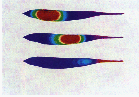
Figure 12.6:
Potentials on the surface of the electric
fish model as a conducting object moves from head (left) to tail (right) of
the fish, keeping 3cm from the midline (above the paper).
Figure 12.7:
Envelope of Voltage Differences Along Midline of the Fish, for
20 Object Positions, Each  Above Mid-plane
Guy Robinson
Wed Mar 1 10:19:35 EST 1995
12.2.4 Summary
Next:
12.3 Transonic Flow
Up:
Simulation of the
Previous:
12.2.3 Results
The BEM algorithm was written as a DIME application [Williams:90b;90c]
by Roy Williams,
Brian Rasnow of the Biology
Division, and Chris Assad of the
Engineering Division.
Guy Robinson
Wed Mar 1 10:19:35 EST 1995
12.3 Transonic Flow
Next:
12.3.1 Compressible Flow Algorithm
Up:
Irregular Loosely Synchronous
Previous:
12.2.4 Summary
Unstructured meshes have been widely used for calculations with
conventional sequential machines. Jameson [Jameson:86a;86b]
uses explicit
finite-element-based
schemes on fully
unstructured tetrahedral meshes to solve for the flow around a complete
aircraft, and other workers [
Dannenhoffer:89a
], [
Holmes:86a
],
[Lohner:84a;85a;86a]
have used unstructured triangular meshes. Jameson
and others [Jameson:87a;87b],
[
Mavriplis:88a
], [
Perez:86a
], [
Usab:83a
] have used
multigrid methods
to accelerate
convergence
. For this work [
Williams:89b
], we
have used the two-dimensional explicit algorithm of Jameson and
Mavriplis [
Mavriplis:88a
].
An explicit update procedure is local, and hence well matched to a massively
parallel distributed machine, whereas an implicit algorithm is more difficult
to parallelize. The implicit step consists of solving a sparse set of linear
equations, where matrix elements are nonzero only for mesh-connected nodes.
Matrix multiplication is easy to parallelize since it is also a local
operation, and the solve may thus be accomplished by an iterative technique
such as conjugate gradient, which consists of repeated matrix
multiplications. If, however, the same solve is to be done repeatedly for
the same mesh, the most efficient (sequential) method is first decomposing
the matrix in some way, resulting in fill-in. In terms of the mesh, this
fill-in represents nonlocal connection between nodes:indeed, if the
matrix were completely filled, the communication time would be proportional to
 for
N
nodes.
for
N
nodes.
Guy Robinson
Wed Mar 1 10:19:35 EST 1995
12.3.1 Compressible Flow Algorithm
Next:
12.3.2 Adaptive Refinement
Up:
12.3 Transonic Flow
Previous:
12.3 Transonic Flow
The governing equations are the Euler equations, which are of advective type
with no diffusion,

where
U
is a vector containing the information about the fluid at a
point. I have used bold symbols to indicate an
information
vector,
or a set of fields describing the state of the fluid. In this
implementation,
U
consists of density, velocity, and specific total
energy (or, equivalently, pressure); it could also include other information
about the state of the fluid such as chemical mixture or ionization data.
F
is the flux vector and has the same structure as
U
in each of
the two coordinate directions.
The numerical algorithm is explained in detail in [
Mavriplis:88a
], so
only an outline is given here. The method uses linear triangular elements to
approximate the field. First, a time step is chosen for each node which is
constrained by a local Courant condition. The calculation consists of two
parts:
-
-
Advection:
At each node, calculate
F
from
U
. Each
element then averages
F
from its neighboring nodes, and calculates the
flux across each edge of the element, which is then added back into the node
opposite the edge. This change in
U
is combined across the
representations of the node in different processors. If the node is at a
boundary which is a hard surface, a modification is made so that no flux of
mass or energy occurs through the surface.
-
-
Artificial Dissipation:
The artificial dissipation is calculated as a combination of approximations
to the Laplacian and the double Laplacian of
U
, involving a combine step
for each. The double Laplacian is only used where the flow is smooth, to
prevent dissipation of strong shocks.
The time stepping is done with a five-stage Runge-Kutta scheme, where the
advection step is done five times, and the dissipation step is done twice.
Since advection takes one communication stage and dissipation two, each full
time step requires nine loosely synchronous communication stages.
Next:
12.3.2 Adaptive Refinement
Up:
12.3 Transonic Flow
Previous:
12.3 Transonic Flow
Guy Robinson
Wed Mar 1 10:19:35 EST 1995
12.3.2 Adaptive Refinement
Next:
12.3.3 Examples
Up:
12.3 Transonic Flow
Previous:
12.3.1 Compressible Flow Algorithm
After the initial transients have dispersed and the flow has settled, the
mesh
may be refined. The criterion used is based on the gradient of
the pressure for deciding which elements are to be refined. The user specifies a
percentage of elements which are to be refined, and a criterion

is calculated for each element. A value  of this criterion
is found such that the given percentage of elements have a value of
of this criterion
is found such that the given percentage of elements have a value of
 greater than
  , and those elements are refined. The
criterion is not simply the gradient of the pressure, because the strongest
shock in the simulation would soak up all the
refinement
leaving weaker
shocks unresolved. With the element area
, and those elements are refined. The
criterion is not simply the gradient of the pressure, because the strongest
shock in the simulation would soak up all the
refinement
leaving weaker
shocks unresolved. With the element area  in the criterion,
regions will ``saturate'' after sufficient refinement, allowing weaker shocks
to be refined.
in the criterion,
regions will ``saturate'' after sufficient refinement, allowing weaker shocks
to be refined.
Guy Robinson
Wed Mar 1 10:19:35 EST 1995
12.3.3 Examples
Next:
12.3.4 Performance
Up:
12.3 Transonic Flow
Previous:
12.3.2 Adaptive Refinement
Figures 10.8 and 10.9 (Color Plates) show the pressure and
computational mesh resulting from Mach 0.8 flow over a NACA0012 airfoil
at 1.25 degrees angle of attack, computed with a 32-processor nCUBE
machine. This problem is that used by the AGARD working group
[
AGARD:83a
] in their benchmarking of compressible flow
algorithms. The mesh has 5135 elements after four stages of
adaptive
refinement. Each processor has about the same
number of elements. In the pressure plot is also shown the sonic line;
the plot agrees well with the AGARD data.
Note the shock about 2/3 of the way downstream from the leading edge,
and the corresponding increase in mesh density there.
Figure 12.8 (Color Plate) shows pressure in a wind-tunnel with a step. A
Mach 3 stream comes in from the left, with a detached bow-shock upstream
from the step. A second shock is attached by a Mach stem to the bow
shock, which is then reflected from the walls of the wind tunnel.
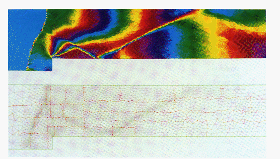
Figure 12.8:
Pressure and mesh for a Mach 3 wind
tunnel with a step. The red lines in the mesh separate processor domains.
The mesh has been dynamically adapted and load-balanced with orthogonal
recursive bisection.
Notice how the mesh density is much greater in the neighborhood of the
shocks and at the step where the pressure gradient is high. This
computation was performed on 32 processors of a Symult machine.
Guy Robinson
Wed Mar 1 10:19:35 EST 1995
12.3.4 Performance
Next:
12.3.5 Summary
Up:
12.3 Transonic Flow
Previous:
12.3.3 Examples
The efficiency of any parallel algorithm increases as the computational
load dominates the communication load [
Williams:90a
]. In the case
of a domain-decomposed mesh, the computational time depends on the
number of elements per processor, and the communication time on the
number of nodes at the boundary of the processor domain. If there are
N
elements in total, distributed among
n
processors, we expect the
computation to go as  and the communication as the square root of
this, so that the efficiency should approach unity as the square root
of
and the communication as the square root of
this, so that the efficiency should approach unity as the square root
of  .
.
We have run the example described above starting with a mesh of 525 elements,
and refining 50% of the elements. In fact, more than 50% will be refined
because of the nature of the refinement algorithm:In practice, it is about
70%. The refinement continues until the memory of the machine runs out.
Figure
12.9
shows timing results. At top right are results for
1, 4, 16, 64, and 256 nCUBE processors. The time taken per simulation
time step is shown for the compressible flow algorithm against number of
elements in the simulation. The curves end when the processor memory is
full. Each processor offers a nominal  memory, but when all the
software and communication buffers are accounted for, there is only about
memory, but when all the
software and communication buffers are accounted for, there is only about
 available for the mesh.
The top left of Figure
12.9
shows the same curves for 1,
4, 16, 64, and 128 Symult processors, and at bottom left the results
for 1, 4, 16, and 32 processors of a Meiko
CS-1 computing
surface. For comparison, the bottom right shows the results for one
head of the CRAY Y-MP,
and also for the Sun Sparcstation.
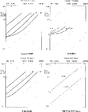
Figure 12.9:
Timings for Transonic Flow
Each figure has diagonal lines to guide the eye; these are lines of
constant time per element. We expect the curves for the sequential machines
to be parallel to these because the code is completely local and the time
should be proportional to the number of elements. For the parallel machines,
we expect the discrepancy from parallel lines to indicate the importance of
communication inefficiency.
Next:
12.3.5 Summary
Up:
12.3 Transonic Flow
Previous:
12.3.3 Examples
Guy Robinson
Wed Mar 1 10:19:35 EST 1995
12.3.5 Summary
Next:
12.4 Tree Codes for
Up:
12.3 Transonic Flow
Previous:
12.3.4 Performance
The transonic flow algorithm was written as a DIME application by
Roy Williams, using the algorithm of A. Jameson of Princeton University and
D. Mavriplis of NASA ICASE
[Williams:89b;90a;90b].
Guy Robinson
Wed Mar 1 10:19:35 EST 1995
12.4 Tree Codes for N-body Simulations
Next:
12.4.1 Oct-Trees
Up:
Irregular Loosely Synchronous
Previous:
12.3.5 Summary
Continuous physical systems must generally be ``discretized'' prior to
analysis with a digital computer. In practice, there are relatively
few ways to discretize a physical system. Finite-element and
finite-difference
approximations are useful
for dealing with partial differential equations in a small number of
dimensions (up to three). If the dimensionality of the independent
variable space is large, however, discretization by finite difference
or finite elements becomes unwieldy. For example, the collisionless
Boltzman equation,

is expressed as a partial differential equation in six independent variables.
A fairly modest discretization of the domain with 100 ``elements'' in each
dimension would result in a system with  elements. A simulation of
this size is out of the question on computers which will be available in the
foreseeable future.
elements. A simulation of
this size is out of the question on computers which will be available in the
foreseeable future.
Fortunately, another means of discretization is available. Particle
Simulation
(or N-body simulation) is
discussed at length by Hockney and Eastwood [
Hockney:81a
]. It is
appropriate for systems like the collisionless and collisional Boltzman
equation, and hence it is applicable to a number of outstanding
problems in astrophysics
, where the basic physical
processes are governed by Newtonian gravity and the Boltzman equation
[
Binney:87a
].
In such simulations, the phase-space density,
f
, is represented by a swarm
of ``particles'', or ``bodies'' which evolve in time according to the
dynamics of Newtonian gravity:

The
3N
second-order, ordinary differential equations
may be integrated in time by a large number of
methods, ranging from the very simple (Euler's method) to the very
complex [
Aarseth:85a
]. The difficulty with using
Equation
12.4
is that a straightforward implementation of
the right-hand sides of these equations requires  operations.
Each of
N
accelerations is the vector sum of
N-1
components, each
of which requires a handful of floating-point operations (including at
least one square-root). Even if one utilizes Newton's second law, one
can cut the total number of operations by half, but the asymptotic
operations.
Each of
N
accelerations is the vector sum of
N-1
components, each
of which requires a handful of floating-point operations (including at
least one square-root). Even if one utilizes Newton's second law, one
can cut the total number of operations by half, but the asymptotic
 behavior remains unchanged. N-body simulations using direct
summation are practical up to a few tens of thousands of bodies on
modern supercomputers. Even the teraflop
performance
promised by parallel computation would only increase this by an order
of magnitude or so. Substantially larger simulations require
alternative methods for evaluating the forces. The fact that gravity
is ``long-range,'' makes rapid evaluation of the forces problematical.
It is not acceptable to simply disregard all bodies beyond a certain
fixed cutoff, because the contribution of distant bodies does not
decrease fast enough to balance the fact that the number of bodies at a
given distance is an increasing function of distance.
behavior remains unchanged. N-body simulations using direct
summation are practical up to a few tens of thousands of bodies on
modern supercomputers. Even the teraflop
performance
promised by parallel computation would only increase this by an order
of magnitude or so. Substantially larger simulations require
alternative methods for evaluating the forces. The fact that gravity
is ``long-range,'' makes rapid evaluation of the forces problematical.
It is not acceptable to simply disregard all bodies beyond a certain
fixed cutoff, because the contribution of distant bodies does not
decrease fast enough to balance the fact that the number of bodies at a
given distance is an increasing function of distance.
Recent algorithmic advances [
Appel:85a
], [
Barnes:86a
],
[
Greengard:87b
], [
Jernighan:89a
] however, have shown that while
it is not acceptable to disregard distant collections of bodies, it is
possible to accurately approximate their contribution without summing all of
the individual components. It has been known since the time of Newton that
the effect of the earth on an apple may be computed by replacing the
countless individual atoms in the earth with a single point-mass located at
the earth's center. The force calculation is then:

Next:
12.4.1 Oct-Trees
Up:
Irregular Loosely Synchronous
Previous:
12.3.5 Summary
Guy Robinson
Wed Mar 1 10:19:35 EST 1995
12.4.1 Oct-Trees
Next:
12.4.2 Computing Forces
Up:
12.4 Tree Codes for
Previous:
12.4 Tree Codes for
There are a number of ways to utilize this fact in a computer
simulation [
Appel:85a
], [
Barnes:86a
], [
Greengard:87b
],
[
Zhao:87a
]. The methods differ in choice of data structure,
level of mathematical rigor, and complexity of the fundamental
interactions. We shall consider an adaptive tree data structure, and
an algorithm that treats each body independently. The algorithm
begins by partitioning space into an oct-tree, that is, a tree whose nodes
correspond to cubical regions of space. Each node may have up to eight
daughter nodes, corresponding to the eight subcubes that are obtained
by dividing in half in each Cartesian
direction.
The tree is defined by the following properties:
-
All terminal nodes of the tree have either one or zero bodies.
-
All nodes with one or zero bodies are terminal.
Oct-trees are somewhat difficult to draw on two-dimensional paper. The
corresponding analog in two dimensions is a quad-tree.
Figure
12.10
a shows a very shallow quad-tree, with each of the
square cells explicitly represented. Figure
12.10
b shows the same
tree in a more compact, ``flattened'' representation. The ``flattened''
representation has a tendency to de-emphasize the importance of the higher
levels of the tree. This is purely an artifact of the graphical
representation. In all cases, the tree consists of both terminal nodes and
internal nodes. Figure
12.11
shows a quad-tree derived from 10,000
bodies distributed at random on a disc.
Figure 12.10:
(a) Expanded and (b) Flat Representation of an Adaptive Tree
Figure 12.11:
10,000 Body Barnes-Hut Tree
The oct-tree
provides a convenient data structure
which allows us to record the properties of the matter distribution on
all length scales. It is especially convenient for astrophysical
systems because it is adaptive. That is, the depth of the tree adjusts
itself automatically to the local particle density. In order to use an
approximation like Equation
12.5
, we need to know certain
properties of the matter distribution in each cell. In the simplest
case, these properties are the mass and center-of-mass of the matter
distribution, but it is possible to use quadrupole moments
[
Hernquist:87a
], or higher-order moments [
Salmon:90a
] for
added accuracy. All of these properties may be computed by a bottom-up
traversal of the tree, combining the properties of the ``daughters'' of
a node to get the properties of the node itself. The time required for
this bottom-up traversal is proportional to the number of internal
nodes in the tree, that is,  .
.
Next:
12.4.2 Computing Forces
Up:
12.4 Tree Codes for
Previous:
12.4 Tree Codes for
Guy Robinson
Wed Mar 1 10:19:35 EST 1995
12.4.2 Computing Forces
Next:
12.4.3 Parallelism in Tree
Up:
12.4 Tree Codes for
Previous:
12.4.1 Oct-Trees
Once the distribution of matter is represented on a number of length scales,
it is possible to use the approximation in Equation
12.5
to
reduce the number of operations required to find the force on a body. The
force on each body is computed independently by a recursive procedure that
traverses the tree from the top down. Beginning at the root of the tree, we
simply apply a
multipole acceptability criterion
(MAC). This tells us
whether Equation
12.5
(or an appropriate higher-order
approximation) is sufficiently accurate. If it is, then we evaluate the
approximation, and eliminate the summation over all the bodies contained
within the node. Otherwise, we proceed recursively to the eight daughter
cells of the node. Whenever we reach a terminal node, we simply compute the
body-body interaction. The procedure is shown schematically in
Figure
12.12
.
Figure 12.12:
The Barnes-Hut Algorithm
The performance of the algorithm depends on how we evaluate the MAC. For
example, one could always answer ``no,'' in which case the performance would
be identical to the  case (although the bookkeeping overhead would be
somewhat higher, and we would not take advantage of Newton's second law).
The specifics of how best to evaluate the MAC would take us far afield
[
Barnes:89d
], [
Makino:90a
], and [
Salmon:92a
].
case (although the bookkeeping overhead would be
somewhat higher, and we would not take advantage of Newton's second law).
The specifics of how best to evaluate the MAC would take us far afield
[
Barnes:89d
], [
Makino:90a
], and [
Salmon:92a
].
Suffice it to say that all methods are based on the idea that the multipole
approximation is accurate when the distance to the cell is large compared to
the size of the cell. Essentially any criterion based on a ratio of
size-of-cell to distance-to-cell will require  -force evaluations
to compute the total force on each body [
Barnes:86a
], [
Salmon:90a
].
Since the forces on all bodies are evaluated independently, the total number
of evaluations is proportional to
-force evaluations
to compute the total force on each body [
Barnes:86a
], [
Salmon:90a
].
Since the forces on all bodies are evaluated independently, the total number
of evaluations is proportional to  , which is a substantial
improvement over the
, which is a substantial
improvement over the  situation that results from a naive evaluation
of Equation
12.3
.
situation that results from a naive evaluation
of Equation
12.3
.
Next:
12.4.3 Parallelism in Tree
Up:
12.4 Tree Codes for
Previous:
12.4.1 Oct-Trees
Guy Robinson
Wed Mar 1 10:19:35 EST 1995
12.4.3 Parallelism in Tree Codes
Next:
12.4.4 Acquiring Locally Essential
Up:
12.4 Tree Codes for
Previous:
12.4.2 Computing Forces
Computational science advances both in hardware and algorithms.
Occasionally, algorithmic advances are of such tremendous significance that
they completely overshadow the striking advances constantly being made by
hardware. Tree codes are just such an algorithmic advance. It is literally
true that a tree code running on a modest workstation can address larger
problems than can the fastest parallel supercomputer running an  algorithm. It is well known [
Fox:84e
], [
Fox:88a
] that parallel
computers can efficiently evaluate the
algorithm. It is well known [
Fox:84e
], [
Fox:88a
] that parallel
computers can efficiently evaluate the  force evaluations required by
direct application of Equation
12.5
. However, this fact is of
limited significance now that a new class of algorithms has changed the
underlying complexity of the problem. If parallel computers are to have an
impact on the N-body problem, then they must be able to efficiently execute
tree codes.
force evaluations required by
direct application of Equation
12.5
. However, this fact is of
limited significance now that a new class of algorithms has changed the
underlying complexity of the problem. If parallel computers are to have an
impact on the N-body problem, then they must be able to efficiently execute
tree codes.
Parallelization of tree codes is a challenging problem. Typical
astrophysical simulations are highly inhomogeneous. Spatial densities can
vary by a factor of  or more through the computational domain. The
tree must be adaptive to deal with such a large dynamic range in densities,
that is, it must be deep in regions of high particle density, and shallow in
regions of low particle density. Furthermore, the structure of the
inhomogeneities is often dynamic-for example, galaxies form, move, collide, and
merge in cosmological simulations. A fixed tree and/or a fixed decomposition
is not suitable for such a system. Despite these problems, it is possible to
find parallelism in tree codes and to run them efficiently on large parallel
computers [
Fox:89t
], [
Salmon:90a
], [Warren:92a;93a].
or more through the computational domain. The
tree must be adaptive to deal with such a large dynamic range in densities,
that is, it must be deep in regions of high particle density, and shallow in
regions of low particle density. Furthermore, the structure of the
inhomogeneities is often dynamic-for example, galaxies form, move, collide, and
merge in cosmological simulations. A fixed tree and/or a fixed decomposition
is not suitable for such a system. Despite these problems, it is possible to
find parallelism in tree codes and to run them efficiently on large parallel
computers [
Fox:89t
], [
Salmon:90a
], [Warren:92a;93a].
The technique of ``domain decomposition'' has been applied with excellent
results to a number of other problem areas. We have found that a slightly
abstracted concept of domain decomposition is also applicable to tree codes.
Recall that a domain decomposition usually proceeds by ``assigning'' spatial
domains to processors. In designing a parallel program, the precise meaning
of ``assign'' is crucial. We adopt the following ``owner-computes''
definition of a domain:
A domain is a rectangular region of simulation
space. Assignment of a domain to a processor implies that the processor will
be responsible for updating the positions and velocities of all particles
located within that region of simulation space.
We allow that processor
domains might change from one time step to the next, based, presumably, on
load-balancing considerations.
Processor domains are chosen using orthogonal recursive
bisection,
or ORB (see
Section
11.1.5
). Recall that ORB tries repeatedly to split
some measure of the ``load'' in half, and assign the halves to sets of
processors. In the present context, that means finding a coordinate so
that half of the computational ``load'' is associated with particles
above the split, and half is associated with particles below the
split. The result of applying orthogonal recursive bisection to a
system containing two ``galaxies,'' (well-separated regions with high
local particle density) is shown in Figure
12.13
.
Figure 12.13:
Decomposition Resulting from Orthogonal Recursive
Bisection of a System with Two Galaxies
It is a simple matter to record the ``load'' associated with each particle.
For example, one can count interactions, or one could simply read the clock
before and after the force on the particle is computed. Then, in order to
find the splitting coordinate, one simply executes a binary (or more
sophisticated) search, seeking a value of the coordinate for which half of
the per-particle work is above and half is below.
In fact, seeking the exact median coordinate of the per-particle work does
not necessarily guarantee load balance.
It
guarantees load balance
within the force calculation
, but it
does not account for load imbalance that may result during construction
of the tree, or during the other phases of the computation. It is
possible to account for these sources of load imbalance by seeking a
coordinate which is not precisely at the median (i.e.,  percentile), but rather at another percentile. The new target
percentile is found by measuring the actual load imbalance, and
adjusting the target by a small amount on each time step to reduce the
observed load imbalance [
Salmon:90a
].
percentile), but rather at another percentile. The new target
percentile is found by measuring the actual load imbalance, and
adjusting the target by a small amount on each time step to reduce the
observed load imbalance [
Salmon:90a
].
Next:
12.4.4 Acquiring Locally Essential
Up:
12.4 Tree Codes for
Previous:
12.4.2 Computing Forces
Guy Robinson
Wed Mar 1 10:19:35 EST 1995
12.4.4 Acquiring Locally Essential Data
Next:
12.4.5 Comments on Performance
Up:
12.4 Tree Codes for
Previous:
12.4.3 Parallelism in Tree
Many parallel algorithms conform to a pattern of activity that
can loosely be described as:
-
Choose a decomposition-that is, determine which processor is responsible
for updating which data.
-
Communicate-that is, arrange for some data to reside in several
processors. Exactly which data are replicated, and how they are stored
depends on the next phase.
-
Proceed with calculation using an essentially serial
implementation, but restrict the data updated by each processor to
those in the processor's domain.
In this volume, the techniques discussed are structured in this way. Some
important advantages arise from this approach to parallelism. It leads to
modularity and portability, by separating distinct functions into separate
phases. It also allows reuse of sequential code (in the third phase), which
is frequently highly optimized and extensively tested. One drawback of this
approach is the fact that it precludes overlapping of communication
and calculation. We shall not be concerned with overlap of communication and
calculation because communication overhead constitutes a small part of the
overall time in parallel tree code implementations [
Salmon:90a
].
We have already discussed decomposition, and described the use of
orthogonal recursive bisection to determine processor domains. The
next step is the acquisition of ``locally essential data'', that is, the
data that will be needed to compute the forces on the bodies in a local
domain. In other applications one finds that the locally essential
data associated with a domain is itself local. That is, it comes
from a limited region surrounding the processor domain. In the case of
hierarchical N-body simulations, however, the locally essential data is
not restricted to a particular region of space. Nevertheless, the
hierarchical nature of the algorithm guarantees that if a processor's
domain is spatially limited, then any particle within that domain will
not require detailed information about the particle distribution in
distant regions of space. This idea is illustrated in
Figure
12.14
, which shows the parts of the tree that are
required to compute forces on bodies in the grey region. Clearly, the
locally essential data for a limited domain is much smaller than the
total data set (shown in Figure
12.11
). In fact, when the
grain size of the domain is large, that is, when the number of bodies in
the domain is large, the size of the locally essential data set is only
a modest constant factor larger than the local data set itself
[
Salmon:90a
]. This means that the work (both communication and
additional computation) required to obtain and assemble the locally
essential dataset is proportional to the grain size, that is, is
 . In contrast, the work required to compute the forces
in parallel is
. In contrast, the work required to compute the forces
in parallel is  . The ``big-O'' notation can hide
large constants which dominate practical considerations. Typical
astrophysical simulations with
. The ``big-O'' notation can hide
large constants which dominate practical considerations. Typical
astrophysical simulations with  -
- bodies perform
200
500
interactions per body [
Hernquist:87a
],
[
Warren:92a
], and each interaction costs from 30 to 60 floating-point
operations. Thus, there is reason to be optimistic that assembly
of the locally essential data set will not be prohibitively expensive.
bodies perform
200
500
interactions per body [
Hernquist:87a
],
[
Warren:92a
], and each interaction costs from 30 to 60 floating-point
operations. Thus, there is reason to be optimistic that assembly
of the locally essential data set will not be prohibitively expensive.
Figure 12.14:
The Locally Essential Data Needed to Compute Forces in a
Processor Domain, Located in the Lower Left Corner of the System
Determining, in parallel, which data is locally essential for which
processors is a formidable task. Two facts allow us to organize the
communication of data into a regular pattern that guarantees that each
processor receives precisely the locally essential data which it needs.
-
At each level of the orthogonal recursive bisection, the domains are
always rectangles.
-
It is possible to quickly determine whether a given cell's multipole
approximation is acceptable for all particles in a given rectangular domain.
Or, conversely, whether the locally essential data for the domain includes
information contained in the daughters of the given cell. This test is
called the domain multipole acceptability criterion (DMAC).
The procedure by which processors go from having only local data to having
all locally essential data consists of a loop over each of the bisections in
the ORB tree. To initialize the iteration, each processor builds a tree from
its local data. Then, for each bisector, it traverses its tree, applying the
DMAC at each node, using the
complimentary domain
as an argument,
that is, asking whether the given cell contains an approximation that is
sufficient for all bodies in the domain on the other side of the current ORB
bisector. If the DMAC succeeds, the cell is needed on the other side of the
domain, so it is copied to a buffer and queued for transmission. Traversal
of the current branch can stop at this point because no additional
information within the current branch of the local tree can possibly be
necessary on the other side of the bisector. If the DMAC fails, traversal
continues to deeper levels of the tree. This procedure is shown
schematically in code in Table
12.1
.
Table 12.1:
Outline of
BuildLETree
which constructs a locally essential
representation of a tree.
Figure
12.15
shows schematically how some data might travel around
a 16-processor system during execution of the above code.
The second tree traversal in the above code conserves a processor's memory by
reclaiming data which was transmitted through the processor, but which is not
needed by the processor itself, or any other member of its current subset.
In Figure
12.15
, the body sent from processor 0110 through 1110
and 1010 to 1011 would likely be deleted from processor 1110's tree during
the pruning on channel 2, and from 1010's tree during the pruning on
channel 0.
Figure 12.15:
Data Flow in a 16 Processor System. Arrows indicate the flow of
data and are numbered with a decreasing ``channel'' number corresponding to
the bisector being traversed.
The Code requires the existence of a DMAC function. Obviously, the DMAC
depends on the details of the MAC which will eventually be used to traverse
the tree to evaluate forces. Notice, however, that the DMAC must be
evaluated
before
the entire contents of a cell are available in a
particular processor. (This happens whenever the cell itself extends outside
of the processor's domain). Thus, the DMAC must rely on purely geometric
criteria (the size and location of the cell), and cannot depend on, for
example, the
exact location of the center-of-mass of the cell. The DMAC is allowed,
however, to err on the side of caution. That is, it is allowed to return a
negative result about a cell even though subsequent data may reveal that the
cell is indeed acceptable. The penalty for such ``false negatives'' is
degraded performance, as they cause data to be unnecessarily communicated and
assembled into locally essential data
sets.

Figure 12.16:
The Distance Used by the DMAC is Computed by Finding the Shortest
Distance Between the Processor Domain and the Boundary of the Cell.
Because the DMAC must work with considerably less information than the
MAC, it is somewhat easier to categorically describe its behavior.
Figure
12.16
shows schematically how the DMAC is
implemented. Recall that the MAC is based on a ``distance-to-size''
ratio. The distance used by the DMAC is the shortest distance from the
cell to the processor domain. The ``min-distance'' MAC
[Salmon:90a;92a] uses precisely
this distance to decide whether a multipole approximation is
acceptable. Thus, in a sense, the min-distance MAC is best suited to
parallelization because it is equivalent to its own DMAC. The DMAC
generates fewer false-positive decisions. Fortunately, the
min-distance MAC also resolves certain difficulties associated with
more commonly used MACs, and is arguably the best of the ``simple''
MACs [
Salmon:92a
].
Next:
12.4.5 Comments on Performance
Up:
12.4 Tree Codes for
Previous:
12.4.3 Parallelism in Tree
Guy Robinson
Wed Mar 1 10:19:35 EST 1995
12.4.5 Comments on Performance
Next:
Fast Vortex Algorithm
Up:
12.4 Tree Codes for
Previous:
12.4.4 Acquiring Locally Essential
It is possible to generate a huge amount of data related to parallel
performance. One can vary the size of the problem, and/or the number of
processors. Performance can be related to various problem parameters, for
example,
the nonuniformity of the particle distribution. Parallel overheads can be
identified and attributed to communication, load imbalance, synchronization, or
additional calculation in the parallel code [
Salmon:90a
]. All
these provide useful diagnostics and can be used to predict performance
on a variety of machines. However, they also tend to obscure the fact
that the ultimate goal of parallel computation is to perform
simulations larger or faster than would otherwise be possible.
Rather than analyze a large number of statistics, we restrict
ourselves to the following ``bald'' facts.
In 1992, the 512-processor Intel Delta at Caltech evolved two
astrophysical simulations with 17.15 million bodies for approximately
600 time steps. The machine ran at an aggregate speed exceeding
5000 MFLOPS/sec. The systems under study were simulated regions of the
universe 100 Mpc (megaparsec) and 25 Mpc in diameter, which were
initialized with random-density fluctuations consistent with the
``cold dark matter'' hypothesis and the recent results on the
anisotropy of the microwave background radiation. The data from these
runs exceeded 25 Gbytes, and is analyzed in [
Zurek:93a
]. Salmon
and Warren were recipients of the 1992 Gordon Bell Price for
performance in practical parallel processing research.
Guy Robinson
Wed Mar 1 10:19:35 EST 1995
Fast Vortex Algorithm and ParallelComputing
Next:
12.5.1 Vortex Methods
Up:
Irregular Loosely Synchronous
Previous:
12.4.5 Comments on Performance
Vortex methods
are a powerful tool for the
simulation of incompressible flows
at high
Reynolds number. They rely on a discrete Lagrangian representation of
the vorticity field to approximately satisfy the Kelvin and Helmholtz
theorems which govern the dynamics of vorticity for inviscid flows. A
time-splitting technique can be used to include viscous effects. The
diffusion equation is considered separately after convecting the
particles with an inviscid vortex method. In our work, the viscous
effects are represented by the so-called deterministic method. The
approach was extended to problems where a flux of vorticity is used to
enforce the no-slip boundary condition.
In order to accurately compute the viscous transport of vorticity, gradients
need to be well resolved. As the Reynolds number is increased, these
gradients get steeper and more particles are required to achieve the
requisite resolution. In practice, the computing cost associated with the
convection step dictates the number of vortex particles and puts an upper
bound on the Reynolds number that can be simulated with confidence. That
threshold can be increased by reducing the asymptotic time complexity of the
convection step from  to
to  . The nearfield
of every vortex particle is identified. Within that region, the velocity is
computed by considering the pairwise interaction of vortices. The speedup
is achieved by approximating the influence of the rest of the domain, the
farfield. In that context, the interaction of two vortex particles is
treated differently depending on their spatial relation. The resulting
computer code does not lend itself to vectorization but has been successfully
implemented on concurrent computers.
. The nearfield
of every vortex particle is identified. Within that region, the velocity is
computed by considering the pairwise interaction of vortices. The speedup
is achieved by approximating the influence of the rest of the domain, the
farfield. In that context, the interaction of two vortex particles is
treated differently depending on their spatial relation. The resulting
computer code does not lend itself to vectorization but has been successfully
implemented on concurrent computers.
Guy Robinson
Wed Mar 1 10:19:35 EST 1995
12.5.1 Vortex Methods
Next:
12.5.2 Fast Algorithms
Up:
Fast Vortex Algorithm
Previous:
Fast Vortex Algorithm
Vortex methods (see [
Leonard:80a
]) are used to simulate incompressible
flows at high Reynolds number. The two-dimensional inviscid vorticity
equation,
is solved by discretizing the vorticity field into Lagrangian vortex
particles,
where  is the strength or the circulation of the
  particle. For an incompressible flow, the knowledge of the vorticity is
sufficient to reconstruct the velocity field. Using complex notation, the
induced velocity is given by
particle. For an incompressible flow, the knowledge of the vorticity is
sufficient to reconstruct the velocity field. Using complex notation, the
induced velocity is given by
The velocity is evaluated at each particle location and the discrete
Lagrangian elements are simply advected at the local fluid velocity. In this
way, the numerical scheme approximately satisfies Kelvin and Helmholtz
theorems that govern the motion of vortex lines. The numerical
approximations have transformed the original partial differential equation
into a set of
2N
ordinary differential equations,
an
N
-body problem. This class of problems
is encountered in many fields of computational physics, for example,
molecular dynamics,
gravitational
interactions, plasma physics
and, of course,
vortex dynamics.
Guy Robinson
Wed Mar 1 10:19:35 EST 1995
12.5.2 Fast Algorithms
Next:
12.5.3 Hypercube Implementation
Up:
Fast Vortex Algorithm
Previous:
12.5.1 Vortex Methods
When each pairwise interaction is considered, distant and nearby pairs of
vortices are treated with the same care. As a result, a disproportionate
amount of time is spent computing the influence of distant vortices that have
little influence on the velocity of a given particle. This is not to say
that the far field is to be totally ignored since the accumulation of small
contributions can have a significant effect. The key element in making the
velocity evaluation faster is to approximate the influence of the far field
by considering groups of vortices instead of the individual vortices
themselves. When the collective influence of a distant group of vortices is
to be evaluated, the very accurate representation of the group provided by
its vortices can be overlooked and a cruder description that retains only its
most important features can be used. These would be the group location,
circulation, and, possibly, some coarse approximation of its shape and
vorticity distribution.
A convenient approximate representation is based on multipole expansions. It
would be possible to build a fast algorithm by evaluating the multipole
expansion at the location of particles that do not belong to the group. This
is basically the scheme used by Barnes and Hut [
Barnes:86a
] (the
concurrent implementation of this algorithm is discussed in
Section
12.4
). Greengard and Rokhlin [
Greengard:87b
] went a step
further by proposing group-to-group interactions. In this case, the
multipole expansion is transformed into a Taylor series around the center of
the second group, where the influence of the first one is sought. The
expansions provide an accurate representation of the velocity field when the
distance between the groups is large compared to their radii.
One now needs a data structure that is going to facilitate the search for
acceptable approximations. As proposed by Appel [
Appel:85a
], a
binary tree is used. In that framework, a giant cluster sits on top of the
data structure; it includes all the vortex particles. It stores all the
information relevant to the group, that is, its location, its radius, and the
coefficients of the multipole expansion. In addition, it carries the address
of its two children, each of them responsible for approximately half of the
vortices of the parent group. Whenever smaller groups are sought, these
pointers are used to rapidly access the relevant information. The children
carry the description of their own group of vortices and are themselves
pointing at two smaller groups, their own children, the grandchildren of the
patriarchal group. More subgroups are created by equally dividing the
vortices of the parent groups along the ``x'' and ``y'' axis alternatively.
This splitting process stops when all groups have approximately  vortices. Then, instead of pointing toward two smaller groups, the parent
node points toward a list of vortices. This data structure provides a quick
way to access groups, from the largest to the smallest ones, and ultimately
to the individual vortices themselves. Appel's data structure is Lagrangian
since it is built on top of the vortices and moves with them. As a result,
it can be used for many time steps.
vortices. Then, instead of pointing toward two smaller groups, the parent
node points toward a list of vortices. This data structure provides a quick
way to access groups, from the largest to the smallest ones, and ultimately
to the individual vortices themselves. Appel's data structure is Lagrangian
since it is built on top of the vortices and moves with them. As a result,
it can be used for many time steps.
Comparing the speed of this algorithm with the classical  approach, the crossover occurs for as few as 150 vortices. At this point,
the extra cost of maintaining the data structure is balanced by the savings
associated with the approximate treatment of the far field. When
N
is
increased further, the savings outweigh the extra bookkeeping and the
proposed algorithm is faster than its competitor by a margin that increases
with the number of vortices.
approach, the crossover occurs for as few as 150 vortices. At this point,
the extra cost of maintaining the data structure is balanced by the savings
associated with the approximate treatment of the far field. When
N
is
increased further, the savings outweigh the extra bookkeeping and the
proposed algorithm is faster than its competitor by a margin that increases
with the number of vortices.
Next:
12.5.3 Hypercube Implementation
Up:
Fast Vortex Algorithm
Previous:
12.5.1 Vortex Methods
Guy Robinson
Wed Mar 1 10:19:35 EST 1995
12.5.3 Hypercube Implementation
Next:
12.5.4 Efficiency of Parallel
Up:
Fast Vortex Algorithm
Previous:
12.5.2 Fast Algorithms
The global nature of the  approach has made its parallel
implementation fairly straightforward (see [
Fox:88a
]). However,
as we have already seen in Section
12.4
, that character was
drastically changed by the fast algorithm as it introduced a strong
component of locality. Globality is still present since the influence
of particle is felt throughout the domain, but more care and
computational effort is given to its near field. The fast parallel
algorithm has to reflect that dual nature, otherwise an efficient
implementation will never be obtained. Moreover, the domain
decomposition can no longer ignore the spatial distribution of the
vortices. Nearby vortices are strongly coupled computationally, so it
makes sense to assign them to the same processor. Binary bisection is
used in the host to spatially decompose the domain. Then, only the
vortices are sent to the processors where a binary tree is locally
built on top of them. For example, Figure
12.17
shows the
portion of the data structure assigned to processor
1
in a
4-processor environment.
approach has made its parallel
implementation fairly straightforward (see [
Fox:88a
]). However,
as we have already seen in Section
12.4
, that character was
drastically changed by the fast algorithm as it introduced a strong
component of locality. Globality is still present since the influence
of particle is felt throughout the domain, but more care and
computational effort is given to its near field. The fast parallel
algorithm has to reflect that dual nature, otherwise an efficient
implementation will never be obtained. Moreover, the domain
decomposition can no longer ignore the spatial distribution of the
vortices. Nearby vortices are strongly coupled computationally, so it
makes sense to assign them to the same processor. Binary bisection is
used in the host to spatially decompose the domain. Then, only the
vortices are sent to the processors where a binary tree is locally
built on top of them. For example, Figure
12.17
shows the
portion of the data structure assigned to processor
1
in a
4-processor environment.
In a fast algorithm context, sending a copy of local data structure to
half the other processors does not necessarily result in a load
balanced
implementation. The work associated with
processor-to-processor interactions now depends on their respective
location in physical space. A processor whose vortices are located at
the center of the domain is involved in more costly interactions than a
peripheral processor. To achieve the best possible load balancing,
that central processor could send a copy of its data to more than half
of the other processors and hence itself be responsible for a smaller
fraction of the work associated with its vortices.
Before a decision is made on which one is going to visit and which
to receive, we minimize the number of pairs of processors that
need to exchange their data structure. Following the domain
decomposition, the portion of the data structure that sits above the
subtrees is not present anywhere in the hypercube. That gap is filled
by broadcasting the description of the largest group of every
processor. By limiting the broadcast
to one group per
processor, a small amount of data is actually exchanged but, as seen on
Figure
12.18
, this step gives every processor a coarse
description of its surroundings and helps it find its place in the
universe.
Figure 12.17:
Data Structure Assigned to Processor 1
Figure 12.18:
Data Structure Known to Processor 1 After Broadcast
If the vortices of processor
A
are far enough from those of processor
B
, it is even possible to use that coarse description to compute the
interaction of
A
and
B
without an additional exchange of
information. The far field of every processor can be quickly disposed of.
After thinking globally, one now has to act locally; if the vortices of
A
are adjacent to those of
B
, a more detailed description of
their vorticity field is needed to compute their mutual influence.
This requires a transfer of information from either
A
to
B
or
from
B
to
A
. In the latter case, most of the work involved in
the
A-B
interaction takes place in processor
A
. Obviously,
processor
B
should not always send its information away since it would
then remain idle while the rest of the hypercube is working. Load-balancing
concerns will dictate the flow of information.
Next:
12.5.4 Efficiency of Parallel
Up:
Fast Vortex Algorithm
Previous:
12.5.2 Fast Algorithms
Guy Robinson
Wed Mar 1 10:19:35 EST 1995
12.5.4 Efficiency of Parallel Implementation
Next:
12.5.5 Results
Up:
Fast Vortex Algorithm
Previous:
12.5.3 Hypercube Implementation
Since our objective is to compute the flow around a cylinder, the efficiency
of the parallel implementation was tested on such a problem. The region for
which  is uniformly covered with
N
particles. The parallel
efficiency is shown on Figure
12.19
as a function of the
hypercube size. The parallel implementation is fairly robust: The parallel
efficiency,
is uniformly covered with
N
particles. The parallel
efficiency is shown on Figure
12.19
as a function of the
hypercube size. The parallel implementation is fairly robust: The parallel
efficiency,  , remains larger than
  . The number of vortices per
processor was kept roughly constant at
1500
even if the parallel efficiency
is not a strong function of the size of the problem. It is, however, much
more sensitive to the quality of the domain decomposition. The fast parallel
algorithm performs better when all the subdomains have approximately the
same squarish shape or in other words, when the largest group assigned to a
processor is as compact as possible.
. The number of vortices per
processor was kept roughly constant at
1500
even if the parallel efficiency
is not a strong function of the size of the problem. It is, however, much
more sensitive to the quality of the domain decomposition. The fast parallel
algorithm performs better when all the subdomains have approximately the
same squarish shape or in other words, when the largest group assigned to a
processor is as compact as possible.
Figure 12.19:
Parallel Efficiency of the Fast Algorithm
The results of Figure
12.19
were obtained at early times when the
Lagrangian particles are still distributed evenly around the cylinder which
makes the domain decomposition an easier task. At later times, the
distribution of the vortices does not allow the decomposition of the domain
in groups having approximately the same radius and the same number of
vortices. Some subdomains cover a larger region of space and as a result,
the efficiency drops to approximately 0.6. This is mainly due to the fact
that more processors end up in the near field of a processor responsible for
a large group; the request lists are longer and more data has to be moved
between processors.
The sources of overhead corresponding to Figure
12.19
are shown
on Figure
12.20
normalized with the useful work. Load imbalance,
the largest overhead contributor, is defined as the difference between the
maximum useful work reported by a processor and the average useful work per
processor. Further, the extra work includes the time spent making a copy of
one's own data structure, the time required to absorb the returning
information, and the work that was duplicated in all processors, namely, the
search for acceptable interactions in the upper portion of the tree and the
subsequent creation of the request lists. The remaining overhead has been
lumped under communication time although most of it is probably idle time (or
synchronization time) that was not included in the definition of load
imbalance.
Figure 12.20:
Load Imbalance (solid), Communication and Synchronization Time
(dash), and Extra Work (dot-dash) as a Function of the Number of
Processors
We expected that as
P
increases, the near field of a processor would
eventually contain a fixed number of neighboring processors. The number of
messages and the load imbalance would then reach an asymptote and the loss of
efficiency would be driven by the much smaller communication and extra times.
However, this has yet to happen at 32 processors and the communication time
is already starting to make an impact.
Nevertheless, the fast algorithm, its reasonably efficient parallel
implementation and the speed of the Mark III have made possible simulations
with as many as 80,000 vortex particles.
Next:
12.5.5 Results
Up:
Fast Vortex Algorithm
Previous:
12.5.3 Hypercube Implementation
Guy Robinson
Wed Mar 1 10:19:35 EST 1995
12.5.5 Results
Next:
12.6 Cluster Algorithms for
Up:
Fast Vortex Algorithm
Previous:
12.5.4 Efficiency of Parallel
These 80,000 particles were used to compute the flow past an impulsively
started cylinder. Figure 12.21 (Color Plate) shows the vorticity field after
five time units, meaning that the cylinder has been displaced by five radii;
the Reynolds number is 3000. The pair of primary eddies induced by the
body's motion is clearly visible along with a number of small structures
produced by the interaction of the wake with the rear portion of the cylinder.
It should be noted that symmetry has been enforced in the simulation.
Streamlines derived from this vorticity distribution are presented in
Figure
12.22
and compared with Bouard and Coutanceau's flow
visualization [
Bouard:80a
] obtained at the same dimensionless time and
Reynolds number.
Figure 12.21:
Vorticity field for Re = 3000 at time =
5.0
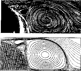
Figure 12.22:
Comparison of Computed Streamlines with Bouard and Coutanceau
Experimental Flow Visualization at
Re=3000
and 
Guy Robinson
Wed Mar 1 10:19:35 EST 1995
12.6 Cluster Algorithms for Spin Models
Next:
12.6.1 Monte Carlo Calculations
Up:
Irregular Loosely Synchronous
Previous:
12.5.5 Results
Guy Robinson
Wed Mar 1 10:19:35 EST 1995
12.6.1 Monte Carlo Calculations of Spin Models
Next:
12.6.2 Cluster Algorithms
Up:
12.6 Cluster Algorithms for
Previous:
12.6 Cluster Algorithms for
The goal of computer simulations of spin models
is
to generate configurations of spins typical of statistical equilibrium
and measure physical observables on this ensemble of configurations.
The generation of configurations is traditionally performed by Monte
Carlo
methods such as the
Metropolis
algorithm [
Metropolis:53a
], which
produce configurations with a probability given by the Boltzmann
distribution  , where
  is the action, or
energy, of the system in configuration
is the action, or
energy, of the system in configuration  , and
, and  is the
inverse temperature. One of the main problems with these methods in
practice is that successive configurations are not statistically
independent, but rather are correlated with some autocorrelation time,
is the
inverse temperature. One of the main problems with these methods in
practice is that successive configurations are not statistically
independent, but rather are correlated with some autocorrelation time,
 , between effectively independent configurations.
A key feature of traditional (Metropolislike) Monte Carlo algorithms is
that the updates are
local
(i.e., one spin at a time is updated), and
its new value depends only on the values of spins which affect its
contribution to the action, that is, only on local (usually nearest
neighbor) spins. Thus, in a single step of the algorithm, information about
the state of a spin is transmitted only to its nearest neighbors. In order
for the system to reach a new effectively independent configuration, this
information must travel a distance of order the (static or spatial)
correlation length
 . As the information
executes a random walk around the lattice, one would suppose that the
autocorrelation time
. As the information
executes a random walk around the lattice, one would suppose that the
autocorrelation time  . However, in general,
  , where
z
is called the dynamical critical exponent.
Almost all numerical simulations of spin models have measured
, where
z
is called the dynamical critical exponent.
Almost all numerical simulations of spin models have measured  for local update algorithms. (See also Sections
4.3
,
4.4
,
7.3
,
12.6
, and
14.2
).
for local update algorithms. (See also Sections
4.3
,
4.4
,
7.3
,
12.6
, and
14.2
).
For a spin model with a phase transition,
as
the inverse temperature  approaches the critical value,
  diverges to infinity so that the computational efficiency rapidly goes
to zero! This behavior is called
critical slowing down
(CSD),
and until very recently it has plagued Monte Carlo simulations of
statistical mechanical systems, in particular spin models, at or near
their phase transitions. Recently, however, several new ``cluster
algorithms'' have been introduced which decrease
z
dramatically by
performing
nonlocal
spin updates, thus reducing (or even
eliminating) CSD and facilitating much more efficient computer
simulations.
diverges to infinity so that the computational efficiency rapidly goes
to zero! This behavior is called
critical slowing down
(CSD),
and until very recently it has plagued Monte Carlo simulations of
statistical mechanical systems, in particular spin models, at or near
their phase transitions. Recently, however, several new ``cluster
algorithms'' have been introduced which decrease
z
dramatically by
performing
nonlocal
spin updates, thus reducing (or even
eliminating) CSD and facilitating much more efficient computer
simulations.
Next:
12.6.2 Cluster Algorithms
Up:
12.6 Cluster Algorithms for
Previous:
12.6 Cluster Algorithms for
Guy Robinson
Wed Mar 1 10:19:35 EST 1995
12.6.2 Cluster Algorithms
Next:
12.6.3 Parallel Cluster Algorithms
Up:
12.6 Cluster Algorithms for
Previous:
12.6.1 Monte Carlo Calculations
The aim of the cluster
update algorithms is to
find a suitable collection of spins which can be flipped with
relatively little cost in energy. We could obtain nonlocal updating
very simply by using the standard Metropolis Monte Carlo algorithm to
flip randomly selected bunches of spins, but then the acceptance would
be tiny. Therefore, we need a method which picks sensible bunches or
clusters of spins to be updated. The first such algorithm was proposed
by Swendsen and Wang [
Swendsen:87a
], and was based on an
equivalence between a Potts spin model [
Potts:52a
], [
Wu:82a
]
and percolation models [
Stauffer:78a
], [
Essam:80a
], for which
cluster properties play a fundamental role.
The Potts model
is a very simple spin model of a
ferromagnet, in which the spins can take
q
different values. The
case
q=2
is just the well-known Ising model. In the Swendsen and
Wang algorithm, clusters of spins are created by introducing bonds
between neighboring spins with probability  if the two
spins are the same, and zero if they are not. All such clusters are
created and then updated by choosing a random new spin value for each
cluster and assigning it to all the spins in that cluster.
if the two
spins are the same, and zero if they are not. All such clusters are
created and then updated by choosing a random new spin value for each
cluster and assigning it to all the spins in that cluster.
A variant of this algorithm, for which only a single cluster is
constructed and updated at each sweep, has been proposed by Wolff
[
Wolff:89a
]. The implementation of this algorithm is shown in
Figures 12.23 through 12.25 (Color Plates), which show a
q=3
Potts model at its critical temperature, with different colors
representing the three different spin values. From the starting
configuration (Figure 12.23 (Color Plate)), we choose a site at random,
and construct a cluster around it by bonding together neighboring sites
with the appropriate probabilities (Figure 12.24 (Color Plate)). All
sites in this cluster are then given the same new spin value, producing
the new configuration shown in Figure 12.25 (Color Plate), which is
obviously far less correlated with the initial configuration than the
result of a single Metropolis update (Figure 12.26 (Color Plate)).
Although Wolff's method is probably the best
sequential
cluster
algorithm, the Swendsen and Wang algorithm seems to be better suited
for parallelization, since it involves the entire lattice rather than
just a single cluster. We have, therefore, concentrated our attention
on parallelizing the method of Swendsen and Wang, where
all
the
clusters must be identified and labelled.

Figure 12_23:
Initial configuration of 3-state Potts
spins on which Wolff Algorithm is to be applied.
Figure 12_24:
Configuration of figure 12.23 with bonds
of cluster constructed by Wolff Algorithm indicated in yellow.
Figure 12_25:
Results of Wolff Algorithm applied to
spin configuration in color Figure 12.23- all spins in cluster flipped to
same new value (in this case from blue to red).
Figure 12_26:
Results of Metropolis Algorithm applied
to spin configuration in Figure 12.23 - only a few single spins flipped.
First we outline a sequential method for labelling clusters, the so-called
``ants in the labyrinth'' algorithm. The reason for its name is that we can
visualize the algorithm as follows [
Dewar:87a
]. An ant is put somewhere
on the lattice, and notes which of the neighboring sites are connected to the
site it is on. At the next time step, this ant places children on each of
these connected sites which are not already occupied. The children then
proceed to reproduce likewise until the entire cluster is populated. In
order to label all the clusters, we start by giving every site a negative
label, set the initial cluster label to be zero, and then loop through all
the sites in turn. If a site's label is negative, then the site has not
already been assigned to a cluster so we place an ant on this site, give it
the current cluster label, and let it reproduce, passing the label on to all
its offspring. When this cluster is identified, we increment the cluster
label and carry on repeating the ant-colony birth, growth, and death cycle
until all the clusters have been identified.
Next:
12.6.3 Parallel Cluster Algorithms
Up:
12.6 Cluster Algorithms for
Previous:
12.6.1 Monte Carlo Calculations
Guy Robinson
Wed Mar 1 10:19:35 EST 1995
12.6.3 Parallel Cluster Algorithms
Next:
12.6.4 Self-labelling
Up:
12.6 Cluster Algorithms for
Previous:
12.6.2 Cluster Algorithms
As with the percolation models upon which the cluster algorithms are
based, the phase transition in a spin model occurs when the clusters of
bonded spins become large enough to span the entire lattice. Thus,
near criticality (which in most cases is where we want to perform the
simulation), clusters come in all sizes, from order
N
(where
N
is
the number of sites in the lattice) right down to a single site. The
highly irregular and nonlocal nature of the clusters means that
cluster update algorithms do not vectorize well and hence give poor
performance on vector machines. On this problem, a CRAY X-MP
is only about ten times faster than a Sun 4 workstation. The
irregularity of the clusters also means that SIMD machines are not well
suited to this problem [Apostolakis:92a;93a],
[
Baillie:91a
], [
Brower:91a
], whereas
for the Metropolis
type algorithms, they are
perhaps the best machines available. It therefore appears that the
optimum performance for this type of problem will come from MIMD
parallel computers.
A parallel cluster algorithm involves distributing the lattice onto an array
of processors using the usual domain decomposition. Clearly, a sequential
algorithm can be used to label the clusters on each processor, but we need a
procedure for converting these labels to their correct
global
values.
We need to be able to tell many processors, which may be any distance apart,
that some of their clusters are actually the same, to agree on which of the
many different local labels for a given cluster should be assigned to be the
global cluster label, and to pass this label to all the processors containing
a part of that cluster. We have implemented two such algorithms,
``self-labelling''
and ``global equivalencing''
[
Baillie:91a
], [
Coddington:90a
].
Guy Robinson
Wed Mar 1 10:19:35 EST 1995
12.6.4 Self-labelling
Next:
12.6.5 Global Equivalencing
Up:
12.6 Cluster Algorithms for
Previous:
12.6.3 Parallel Cluster Algorithms
We shall refer to this algorithm as ``self-labelling,'' since each site
figures out which cluster it is in by itself from local information.
This method has also been referred to as ``local label propagation''
[
Brower:91a
], [
Flanigan:92a
].
We begin by assigning each site,
i
, a unique cluster label,  . In
practice, this is simply chosen as the position of that site in the lattice.
At each step of the algorithm in parallel, every site looks in turn at each
of its neighbors in the positive directions. If it is bonded to a
neighboring site,
n
, which has a different cluster label,
. In
practice, this is simply chosen as the position of that site in the lattice.
At each step of the algorithm in parallel, every site looks in turn at each
of its neighbors in the positive directions. If it is bonded to a
neighboring site,
n
, which has a different cluster label,  , then both
 and
and  are set to the minimum of the two. This is continued until
nothing changes, by which time all the clusters will have been labelled with
the minimum initial label of all the sites in the cluster. Note that
checking termination of the algorithm involves each processor sending a
termination flag (finished or not finished) to every other processor after
each step, which can become very costly for a large processor array. This is
an SIMD algorithm and can, therefore, be run on machines like the AMT DAP and
TMC Connection Machine.
However, the SIMD
nature of these computers leads to very poor load balancing. Most
processors end up waiting for the few in the largest cluster which are
the last to finish. We implemented this on the AMT DAP and obtained
only about 20% efficiency.
are set to the minimum of the two. This is continued until
nothing changes, by which time all the clusters will have been labelled with
the minimum initial label of all the sites in the cluster. Note that
checking termination of the algorithm involves each processor sending a
termination flag (finished or not finished) to every other processor after
each step, which can become very costly for a large processor array. This is
an SIMD algorithm and can, therefore, be run on machines like the AMT DAP and
TMC Connection Machine.
However, the SIMD
nature of these computers leads to very poor load balancing. Most
processors end up waiting for the few in the largest cluster which are
the last to finish. We implemented this on the AMT DAP and obtained
only about 20% efficiency.
We can improve this method on a MIMD machine by using a faster
sequential algorithm, such as ``ants in the labyrinth,'' to label the
clusters in the sublattice on each processor, and then just use
self-labelling on the sites at the edges of each processor to
eventually arrive at the global cluster labels [
Baillie:91a
],
[
Coddington:90a
], [
Flanigan:92a
]. The number of steps
required to do the self-labelling will depend on the largest cluster
which, at the phase transition, will generally span the entire
lattice. The number of self-labelling steps will therefore be of the
order of the maximum distance between processors, which for a square
array of
P
processors is just  . Hence, the amount of
communication (and calculation) involved in doing the self-labelling,
which is proportional to the number of iterations times the perimeter
of the sublattice, behaves as
L
for an
. Hence, the amount of
communication (and calculation) involved in doing the self-labelling,
which is proportional to the number of iterations times the perimeter
of the sublattice, behaves as
L
for an  lattice; whereas, the time taken on each processor to do the local
cluster labelling is proportional to the area of the sublattice, which
is
lattice; whereas, the time taken on each processor to do the local
cluster labelling is proportional to the area of the sublattice, which
is  . Therefore, as long as
L
is substantially greater than
the number of processors, we can expect to obtain a reasonable
speedup. Of course, this algorithm suffers from the same type of load
imbalance as the SIMD version. However, in this case, it is much less
severe since most of the work is done with ``ants in the labyrinth,''
which is well load balanced.
The speedups obtained
on the Symult 2010, for a variety of lattice sizes, are shown in
Figure
12.27
. The dashed line indicates perfect speedup
(i.e., 100% efficiency). The lattice sizes for which we actually need
large numbers of processors are of the order of
. Therefore, as long as
L
is substantially greater than
the number of processors, we can expect to obtain a reasonable
speedup. Of course, this algorithm suffers from the same type of load
imbalance as the SIMD version. However, in this case, it is much less
severe since most of the work is done with ``ants in the labyrinth,''
which is well load balanced.
The speedups obtained
on the Symult 2010, for a variety of lattice sizes, are shown in
Figure
12.27
. The dashed line indicates perfect speedup
(i.e., 100% efficiency). The lattice sizes for which we actually need
large numbers of processors are of the order of  or greater, and
we can see that running on 64 nodes (or running multiple simulations of
64 nodes each) gives us quite acceptable efficiencies of about 70% for
or greater, and
we can see that running on 64 nodes (or running multiple simulations of
64 nodes each) gives us quite acceptable efficiencies of about 70% for
 and 80% for
  .
.
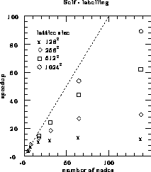
Figure 12.27:
Speedups for Self-Labelling Algorithm
Next:
12.6.5 Global Equivalencing
Up:
12.6 Cluster Algorithms for
Previous:
12.6.3 Parallel Cluster Algorithms
Guy Robinson
Wed Mar 1 10:19:35 EST 1995
12.6.5 Global Equivalencing
Next:
12.6.6 Other Algorithms
Up:
12.6 Cluster Algorithms for
Previous:
12.6.4 Self-labelling
In this method we again use the fastest sequential algorithm to identify the
clusters in the sublattice on every processor. Each processor then looks at
the labels of sites along the edges of the neighboring processors in the
positive directions, and works out which ones are connected and should be
matched up. These lists of ``equivalences'' are all passed to one of
the processors, which uses an algorithm for finding equivalence classes
[
Knuth:68a
], [
Press:86a
] (which, in this case, are the global
cluster labels) to match up the connected clusters. This processor
then broadcasts the results back to all the other processors.
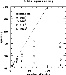
Figure 12.28:
Speedups for Global Equivalencing Algorithm
This part of the algorithm is purely sequential, and is thus a potentially
disastrous bottleneck for large numbers of processors. It also requires
this processor to have a large amount of memory in which to store all the
labels from every other processor. The amount of work involved in doing the
global matchup is proportional to
P
times the perimeter of the
sublattice on each processor, or  so that the efficiency
should be less than for self-labelling; although, we might still
expect reasonable speedups if the number of processors is not extremely
large. The speedups obtained on the Symult 2010 for a variety of
lattice sizes are shown in Figure
12.28
. The figure for
so that the efficiency
should be less than for self-labelling; although, we might still
expect reasonable speedups if the number of processors is not extremely
large. The speedups obtained on the Symult 2010 for a variety of
lattice sizes are shown in Figure
12.28
. The figure for
 on 128 processors is missing due to memory constraints. Global
equivalencing gives about the same speedups as self-labelling for small
numbers of processors, but as expected self-labelling
does much better as the number of processors increases.
on 128 processors is missing due to memory constraints. Global
equivalencing gives about the same speedups as self-labelling for small
numbers of processors, but as expected self-labelling
does much better as the number of processors increases.
Guy Robinson
Wed Mar 1 10:19:35 EST 1995
12.6.6 Other Algorithms
Next:
12.6.7 Summary
Up:
12.6 Cluster Algorithms for
Previous:
12.6.5 Global Equivalencing
The problem of labelling clusters of spins is an example of a standard
graph problem known as
connected component labelling
[
Horowitz:78a
]. Another important instance occurs in image
analysis, in identifying and labelling the connected components of a
binary or multicolored image composed of an array of pixels
[
Rosenfeld:82a
]. There have been a number of parallel algorithms
implemented for this problem [
Alnuweiri:92a
] [
Cypher:89a
],
[
Embrechts:89a
], [
Woo:89a
]. The most promising of these
parallel algorithms for spin models has a hierarchical
divide-and-conquer approach [
Baillie:91a
], [
Embrechts:89a
].
The processor array is divided up into smaller subarrays of, for
example,  processors. In each subarray, the processors look
at the edges of their neighbors for clusters which are connected across
processor boundaries. As in global equivalencing, these equivalences
are all passed to one of the nodes of the subarray, which places them
in equivalence classes. The results of these partial matchings are
similarly combined on each
processors. In each subarray, the processors look
at the edges of their neighbors for clusters which are connected across
processor boundaries. As in global equivalencing, these equivalences
are all passed to one of the nodes of the subarray, which places them
in equivalence classes. The results of these partial matchings are
similarly combined on each  subarray, and this process is
continued until finally all the partial results are merged together on
a single processor to give the global cluster values.
subarray, and this process is
continued until finally all the partial results are merged together on
a single processor to give the global cluster values.
Finally, we should mention the trivial parallelization technique of
running independent Monte Carlo
simulations on
different processors. This method works well until the lattice size
gets too big to fit into the memory of each node. In the case of the
Potts model, for example, only lattices of size less than about  or
or  will fit into 1 Mbyte, though most other spin models are more
complicated and more memory-intensive. The smaller lattices which are
seen to give poor speedups in Figure
12.27
and
Figure
12.28
can be run with 100% efficiency in this
way. Note, of course, that this requires an MIMD computer. In fact,
we have used this method to calculate the dynamical critical exponents
of various cluster algorithms for Potts models [Baillie:90m;91b],
[
Coddington:92a
] (see
Section
4.4.3
).
will fit into 1 Mbyte, though most other spin models are more
complicated and more memory-intensive. The smaller lattices which are
seen to give poor speedups in Figure
12.27
and
Figure
12.28
can be run with 100% efficiency in this
way. Note, of course, that this requires an MIMD computer. In fact,
we have used this method to calculate the dynamical critical exponents
of various cluster algorithms for Potts models [Baillie:90m;91b],
[
Coddington:92a
] (see
Section
4.4.3
).
Next:
12.6.7 Summary
Up:
12.6 Cluster Algorithms for
Previous:
12.6.5 Global Equivalencing
Guy Robinson
Wed Mar 1 10:19:35 EST 1995
12.6.7 Summary
Next:
12.7 Sorting
Up:
12.6 Cluster Algorithms for
Previous:
12.6.6 Other Algorithms
This research was performed by C. F. Baillie, P. D. Coddington,
J. Apostolakis, and E. Marinari.
Guy Robinson
Wed Mar 1 10:19:35 EST 1995
12.7 Sorting
Next:
12.7.1 The Merge Strategy
Up:
Irregular Loosely Synchronous
Previous:
12.6.7 Summary
This section discusses
sorting
:
the rearrangement of
data into some set sequential order. Sorting is a common component of
many applications and so it is important to do it well in parallel.
Quicksort
(to be discussed below) is fundamentally a
divide-and-conquer
algorithm and the parallel
version is closely related to the recursive bisection
algorithm discussed in Section
11.1
. Here, we have
concentrated on the best general-purpose sorting algorithms:
bitonic
,
shellsort
,
and
quicksort
. No
special properties of the list are exploited. If the list to be sorted
has special properties, such as a known distribution (e.g., random
numbers
with a flat distribution between 0 and 1)
or high degeneracy (many redundant items, e.g., text files), then other
strategies can be faster. In the case of known data distribution, a
bucketsort strategy (e.g., radix sort) is best, while the case of high
degeneracy is best handled by the distribution counting method
([Knuth:73a, pp. 379-81]).
The ideas presented here are appropriate for MIMD machines and are somewhat
specific to hypercubes (we will assume  processors), but can easily be
extended to other topologies.
processors), but can easily be
extended to other topologies.
There are two ways to measure the quality of a concurrent algorithm.
The first may be termed ``speed at any cost,'' and here one optimizes
for the highest absolute speed possible for a fixed-size problem. The
other we can call ``speed per unit cost,'' where one, in addition to
speed, worries about efficient use of the parallel machine. It is
interesting that in sorting, different algorithms are appropriate
depending upon which criterion is employed. If one is interested only
in absolute speed, then one should pay for a very large parallel
machine and run the bitonic
algorithm. This
algorithm, however, is inefficient. If efficiency also matters, then
one should only buy a much smaller parallel machine and use the much
more efficient shellsort or quicksort algorithms.
Another way of saying this is: for a
fixed-size
parallel computer
(the realistic case), quicksort and shellsort are actually the
fastest
algorithms on all but the smallest problem sizes. We
continue to find the misconception that ``Everyone knows that the bitonic
algorithm is fastest for sorting.'' This is
not
true for most
combinations of machine size and list size.
The data are assumed to initially reside throughout the parallel
computer, spread out in a random, but load-balanced
fashion (i.e., each processor begins with an approximately equal number
of datums). In our experiments, the data were positive integers and
the sorting key was taken to be simply their numeric value. We require
that at the end of the sorting process, the data residing in each node
are sorted internally and these sublists are also sorted globally
across the machine in some way.
Next:
12.7.1 The Merge Strategy
Up:
Irregular Loosely Synchronous
Previous:
12.6.7 Summary
Guy Robinson
Wed Mar 1 10:19:35 EST 1995
12.7.1 The Merge Strategy
Next:
12.7.2 The Bitonic Algorithm
Up:
12.7 Sorting
Previous:
12.7 Sorting
In the merging strategy to be used by our sorting algorithms, the first step
is for each processor to sort its own sublist using some fast algorithm.
We take for this a combined quicksort/insertion sort which is described
in detail as Algorithm Q by Knuth ([Knuth:73a, pp. 118-9]).
Once the local (processor) sort is complete, it must be decided how to
merge all of the sorted lists in order to form one globally sorted
list. This is done in a series of compare-exchange steps. In each
step, two neighboring processors exchange items so that each processor
ends up with a sorted list and all of the items in one processor are
greater than all of the items in the other. Thus, two sorted lists of
m
items each are merged into a sorted list of 2
m
items
(stored collectively in the memory of the two processors). The
compare-exchange algorithm is interesting in its own right, but we do
not have the space here to discuss it. The reader is referred to
Chapter 18 of [
Fox:88a
] for the details.
Guy Robinson
Wed Mar 1 10:19:35 EST 1995
12.7.2 The Bitonic Algorithm
Next:
12.7.3 Shellsort or Diminishing
Up:
12.7 Sorting
Previous:
12.7.1 The Merge Strategy
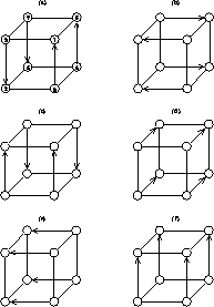
Figure 12.29:
Bitonic Scheme for
d=3
. This figure illustrates the six
compare-exchange steps of the bitonic
algorithm for
d=3
. Each diagram illustrates four compare-exchange processes which happen
simultaneously. The arrows represent a compare-exchange between
two processors. The largest items go to the processor at the point of
the arrow, and the smallest items to the one at the base of the arrow.
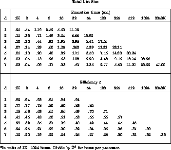
Table 12.2:
Bitonic sort on a hypercube. The rows are labelled by
hypercube size ( ), the columns by number of items
to sort.
), the columns by number of items
to sort.
Many algorithms for sorting on concurrent machines are based upon Batcher's
bitonic sorting
algorithm ([
Batcher:68a
],
[Knuth:73a, pp.232-3]). The first step in the merge
strategy is for each processor to internally sort via quicksort. One
is then left with the problem of constructing a series of
compare-exchange steps which will correctly merge  sorted
sublists. This problem is completely isomorphic to the problem of
sorting a list of
sorted
sublists. This problem is completely isomorphic to the problem of
sorting a list of  items by pairwise comparisons between items.
Each one of our sublist compare-exchange operations is equivalent to a
single compare-exchange between two individual items. The pattern of
compare-exchanges for the bitonic algorithm for the
d=3
case is shown
in Figure
12.29
. More details and a specification of the
bitonic algorithm can be found in Chapter 18 of [
Fox:88a
].
items by pairwise comparisons between items.
Each one of our sublist compare-exchange operations is equivalent to a
single compare-exchange between two individual items. The pattern of
compare-exchanges for the bitonic algorithm for the
d=3
case is shown
in Figure
12.29
. More details and a specification of the
bitonic algorithm can be found in Chapter 18 of [
Fox:88a
].
Table
12.2
shows the actual times and efficiencies for our
implementation of the bitonic algorithm. Results are shown for sorting lists
of sizes  to
to  items on hypercubes with dimensions,
d
, ranging from one (2 nodes) to seven (128 nodes). Efficiencies are
computed by comparing with single-processor times to quicksort the entire
list (we take quicksort to be our benchmark sequential algorithm). The same
information is also shown graphically in Figure
12.30
.
items on hypercubes with dimensions,
d
, ranging from one (2 nodes) to seven (128 nodes). Efficiencies are
computed by comparing with single-processor times to quicksort the entire
list (we take quicksort to be our benchmark sequential algorithm). The same
information is also shown graphically in Figure
12.30
.
Figure 12.30:
The Efficiency of the Bitonic
Algorithm Versus
List Size for Various Size Hypercubes-Labelled by Cube Dimension
d
.
Clearly, the efficiencies fall off rapidly with increasing
d
. From the
standpoint of cost-effectiveness, this algorithm is a failure. On the other
hand, Table
12.2
shows that for fixed-list sizes and increasing
machine size, the execution times continue to decrease. So, from the
speed-at-any-cost point of view, the algorithm is a success. We attribute the
inefficiency of the bitonic algorithm partly to communication overhead and
some load imbalance during the compare-exchanges, but mostly to
nonoptimality of the algorithm itself. In our definition of efficiency we
are comparing the parallel bitonic algorithm to sequential quicksort. In
bitonic, the number of cycles grows quadratically with
d
. This suggests
that efficiency can be improved greatly by using a parallel algorithm that
sorts in fewer operations without sacrificing concurrency.
Next:
12.7.3 Shellsort or Diminishing
Up:
12.7 Sorting
Previous:
12.7.1 The Merge Strategy
Guy Robinson
Wed Mar 1 10:19:35 EST 1995
12.7.3 Shellsort or Diminishing Increment Algorithm
Next:
12.7.4 Quicksort or Samplesort
Up:
12.7 Sorting
Previous:
12.7.2 The Bitonic Algorithm
This algorithm again follows the merge strategy and is motivated by the fact
that
d
compare-exchanges in the
d
different directions of the hypercube
result in an almost-sorted list. Global order is defined via
ringpos
,
that is, the list will end up sorted on an embedded ring in the hypercube.
After the
d
compare-exchange stages, the algorithm switches to a simple
mopping-up stage which is specially designed for almost-sorted lists. This
stage is optimized for moving relatively few items quickly through the
machine and amounts to a parallel bucket brigade algorithm. Details and a
specification of the parallel shellsort
algorithm can be
found in Chapter 18 of [
Fox:88a
].
It turns out that the mop-up algorithm takes advantage of the MIMD nature of
the machine and that this characteristic is crucial to its speed. Only the
few items which need to be moved are examined and processed. The bitonic
algorithm, on the other hand, is natural for a SIMD machine. It involves
much extra work in order to handle the worst case, which rarely occurs.
We refer to this algorithm as shellsort ([
Shell:59a
], [
Knuth:73a
]
pp. 84-5, 102-5) or a diminishing increment algorithm. This is not because
it is a strict concurrent implementation of the sequential namesake, but
because the algorithms are similar in spirit. The important feature of
Shellsort is that in early stages of the sorting process, items take very
large jumps through the list reaching their final destinations in few steps.
As shown in Figure
12.31
, this is exactly what occurs in the
concurrent algorithm.
Figure 12.31:
The Parallel Shellsort on a
d=3
Hypercube. The left side
shows what the algorithm looks like on the cube, the right shows the
same when the cube is regarded as a ring.
The algorithm was implemented and tested with the same data as the bitonic
case. The timings appear in Table
12.3
and are also shown
graphically in Figure
12.32
. This algorithm is much more efficient
than the bitonic algorithm, and offers the prospect of reasonable efficiency
at large
d
. The remaining inefficiency is the result of both communication
overhead and algorithmic nonoptimality relative to quicksort. For most list
sizes, the mop-up time is a small fraction of the total execution time,
though it begins to dominate for very small lists on the largest machine
sizes.
Table 12.3:
Shellsort
Figure:
The Efficiency of the Shellsort Algorithms Versus List Size
for Various Size Hypercubes. The labelling of curves and axes is as
in Figure
12.30
.
Next:
12.7.4 Quicksort or Samplesort
Up:
12.7 Sorting
Previous:
12.7.2 The Bitonic Algorithm
Guy Robinson
Wed Mar 1 10:19:35 EST 1995
12.7.4 Quicksort or Samplesort Algorithm
Next:
Hierarchical Tree-Structures as
Up:
12.7 Sorting
Previous:
12.7.3 Shellsort or Diminishing
The classic quicksort algorithm is a divide-and-conquer sorting method
([
Hoare:62a
], [
Knuth:73a
] pp.118-23). As such, it would seem
to be amenable to a concurrent implementation, and with a slight
modification (actually an improvement of the standard algorithm) this
turns out to be the case.
The standard algorithm begins by picking some item from the list and using
this as the splitting key. A loop is entered which takes the splitting key
and finds the point in the list where this item will ultimately end up once
the sort is completed. This is the first splitting point. While this is
being done, all items in the list which are less than the splitting key are
placed on the low side of the splitting point, and all higher items are
placed on the high side. This completes the first divide. The list
has now been broken into two independent lists, each of which still
needs to be sorted.
The essential idea of the concurrent (hypercube) quicksort is the same. The
first splitting key is chosen (a global step to be described below) and then
the entire list is split, in parallel, between two halves of the hypercube.
All items higher than the splitting key are sent in one direction in the
hypercube, and all items less are sent the other way. The procedure is then
called recursively, splitting each of the subcubes' lists further. As in
Shellsort, the ring-based labelling of the hypercube is used to define global
order. Once
d
splits occur, there remain no further interprocessor splits
to do, and the algorithm continues by switching to the internal quicksort
mentioned earlier. This is illustrated in Figure
12.33
.
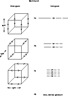
Figure 12.33:
An Illustration of the Parallel Quicksort
So far, we have concentrated on standard quicksort. For quicksort to work
well, even on sequential machines, it is essential that the splitting points
land somewhere near the median of the list. If this isn't true, quicksort
behaves poorly, the usual example being the quadratic time that standard
quicksort takes on almost-sorted lists. To counteract this, it is a good
idea to choose the splitting keys with some care so as to make evenhanded
splits of the list.
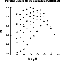
Figure:
Efficiency Data for the Parallel Quicksort described in the
Text. The curves are labelled as in Figure
12.30
and
plotted against the logarithm of the number of items to be sorted.
This becomes much more important on the concurrent computer. In this case,
if the splits are done haphazardly, not only will an excessive number of
operations be necessary, but large load imbalances will also occur.
Therefore, in the concurrent algorithm, the splitting keys are chosen with
some care. One reasonable way to do this is to randomly sample a subset of
the entire list (giving an estimate of the true distribution of the list) and
then pick splitting keys based upon this sample. To save time, all  splitting keys are found at once. This modified algorithm should perhaps be
called
samplesort
and consists of the following steps:
splitting keys are found at once. This modified algorithm should perhaps be
called
samplesort
and consists of the following steps:
-
each processor picks sample of
l
items at random;
-
sort the sample of
 items using the parallel shellsort;
-
choose splitting keys as if this was the entire list;
-
broadcast
splitting keys so that all processors know
all splitting keys;
-
perform the splits in the
d
directions of the hypercube;
-
each processor quicksorts its sublist.
Times and efficiencies for the parallel quicksort algorithm are shown in
Table
12.4
. The efficiencies are also plotted in
Figure
12.34
. In some cases, the parallel quicksort outperforms
the already high performance of the parallel shellsort discussed earlier.
There are two main sources of inefficiency in this algorithm. The first is a
result of the time wasted sorting the sample. The second is due to remaining
load imbalance in the splitting phases. By varying the sample size
l
, we
achieve a trade-off between these two sources of inefficiency. Chapter 18 of
[
Fox:88a
] contains more details regarding the choice of
l
and other
ways to compute splitting points.
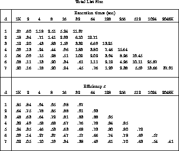
Table 12.4:
Quicksort
Before closing, it may be noted that there exists another way of thinking
about the parallel quicksort/samplesort algorithm. It can be regarded as a
bucketsort, in which each processor of the hypercube comprises one bucket.
In the splitting phase, one attempts to determine reasonable limits for the
 buckets so that approximately equal numbers of items will end up in each
bucket. The splitting process can be thought of as an optimal routing scheme
on the hypercube which brings each item to its correct bucket. So, our
version of quicksort is also a bucketsort in which the bucket limits are
chosen dynamically to match the properties of the particular input list.
buckets so that approximately equal numbers of items will end up in each
bucket. The splitting process can be thought of as an optimal routing scheme
on the hypercube which brings each item to its correct bucket. So, our
version of quicksort is also a bucketsort in which the bucket limits are
chosen dynamically to match the properties of the particular input list.
The sorting work began as a collaboration between Steve Otto and summer
students Ed Felten and Scott Karlin. Ed Felten invented the parallel
Shellsort; Felten and Otto developed the parallel
Quicksort.
Next:
Hierarchical Tree-Structures as
Up:
12.7 Sorting
Previous:
12.7.3 Shellsort or Diminishing
Guy Robinson
Wed Mar 1 10:19:35 EST 1995
Hierarchical Tree-Structures as
Adaptive Meshes
Next:
12.8.1 Introduction
Up:
Irregular Loosely Synchronous
Previous:
12.7.4 Quicksort or Samplesort
Guy Robinson
Wed Mar 1 10:19:35 EST 1995
12.8.1 Introduction
Next:
12.8.2 Adaptive Structures
Up:
Hierarchical Tree-Structures as
Previous:
Hierarchical Tree-Structures as
Two basic types of simulations exist for modelling systems of many
particles: grid-based (point particles indirectly interacting with one
another through the potential calculated from equivalent particle densities
on a mesh) and particle-based (point particles directly interacting with
one another through potentials at their positions calculated from the other
particles in the system). Grid-based solvers traditionally model continuum
problems, such as fluid and gas systems like the one described in
Section
9.3
, and mixed particle-continuum systems. Particle-based
solvers find more use modeling discrete systems such as stars within
galaxies, as discussed in Section
12.4
, or other rarefied gases. Many
different physical systems, including electromagnetic
interactions, gravitational interactions, and fluid vortex interactions all
are governed by Poisson's Equation:

for the gravitational case. To evolve
N
particles in time, the exact
solution to the problem requires calculating the force contribution to each
particle from all other particles at each time step:

The  operation count is prohibitive for simulations of more than a
few thousand particles commonly required to represent astrophysical and
vortex configurations of interest.
operation count is prohibitive for simulations of more than a
few thousand particles commonly required to represent astrophysical and
vortex configurations of interest.
One method of decreasing the operation count utilizes grid-based
solvers which translate the particle problem into a continuum problem
by interpolating the particles onto a mesh representing density and
then solve the discretized equation. Initial implementations were
based upon
fast fourier transform
(FFT)
and
cloud-in-cell
(CIC) methods which can calculate the potential of a
mass distribution on a three-dimensional grid with axes of length
M
in  operations, but at the cost of lower accuracy in
the force resolution. All of these algorithms are discussed
extensively by Hockney and Eastwood [
Hockney:81a
].
operations, but at the cost of lower accuracy in
the force resolution. All of these algorithms are discussed
extensively by Hockney and Eastwood [
Hockney:81a
].
A newer type of grid-based solver for discretized equations classified as a
multilevel or multigrid
method has been in development
for over a decade [
Brandt:77a
], [
Briggs:87b
]. Frequently,
the algorithm utilizes a hierarchy of rectangular meshes on which a
traditional relaxation scheme may be applied, but
multiscale
methods have expanded beyond any
particular type of solver or even grids, per se. Relaxation methods
effectively damp oscillatory error modes whose wave numbers are
comparable to the grid size, but most of the iterations are spent
propagating smooth, low-wave number corrections throughout the system.
Multigrid utilizes this property by resampling the low-wave number
residuals onto secondary, lower-resolution meshes, thereby shifting the
error to higher wave numbers comparable to the grid spacing where
relaxation is effective. The corrections computed on the
lower-resolution meshes are interpolated back onto the original finer
mesh and the combined solutions from the various mesh levels determine
the result.
Many grid-based methods for particle problems have incorporated some
form of local direct-force calculation, such as the
particle-particle/particle-mesh
(PPPM) method or the
method of
local corrections
(MLC), to correct the force on a local subset of
particles. The grid is used to propagate the far-field component of
the force while direct-force calculations provide the near-field
component either completely or as a correction to the ``external''
potential. The computational cost strongly depends on the criterion
used to distinguish near-field objects from far-field objects.
Extremely inhomogeneous systems of densely clustered particles can
deteriorate to nearly  if most of the particles are considered
neighbors requiring direct force computation.
if most of the particles are considered
neighbors requiring direct force computation.
A class of alternative techniques which have been implemented with great
success utilize methods to efficiently calculate and combine the
coefficients of an analytic approximation to the particle forces using
spherical harmonic multipole expansions in three dimensions.
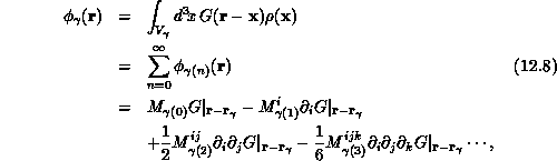
where the multipole moments

 are the disjoint spatial regions, and
  is the Green's
function. Instead of integrating
G
over the volume
is the Green's
function. Instead of integrating
G
over the volume  , one may
compute the potential (and, in a similar manner, the gradient) at any
position by calculating the multipole moments which characterize the
density distribution in each region, evaluating
G
and its derivatives at
, one may
compute the potential (and, in a similar manner, the gradient) at any
position by calculating the multipole moments which characterize the
density distribution in each region, evaluating
G
and its derivatives at
 , and summing over indices. This algorithm is
described more extensively in Section
12.4
.
, and summing over indices. This algorithm is
described more extensively in Section
12.4
.
Not only does spatially sorting
the particles into a
tree-type data structure provide an efficient database for individual
and collective particle information [
Samet:90a
], but the various
algorithms require and utilize the hierarchical grouping of particles
and combined information to calculate the force on each particle from
the multipole moments in  operations or less.
Implementations for three-dimensional problems frequently use an
oct-tree-a
cube divided into eight octants of equal
spatial volume which contain subcubes similarly divided. The cubes
continue to nest until, depending on the algorithm, the cube contains
either zero or one particles or a few particles of equal number to the
other ``terminal'' cells. Binary trees which subdivide the volume with
planes chosen to evenly divide the number of particles instead of the
space also have been used [
Appel:85a
]; a single bifurcation
separates two particles spaced arbitrarily close together while the
oct-tree would require arbitrarily many subcubes refining one
particular region. This approach may produce fewer artifacts by not
imposing an arbitrary rectangular structure onto the simulation, but
construction is more difficult and information about each cut must be
stored and used throughout the computation.
Initial implementations for both grid-based and multipole techniques
normally span the entire volume with a uniform resolution net in which to
catch the result. While this is adequate for homogeneous problems, it
either wastes computational effort and storage or sacrifices accuracy for
problems which exhibit clustering and structure. Many of the algorithms
described above provide enough flexibility to allow adaptive
implementations which can conform to complicated particle distribution or
accuracy constraints.
Next:
12.8.2 Adaptive Structures
Up:
Hierarchical Tree-Structures as
Previous:
Hierarchical Tree-Structures as
Guy Robinson
Wed Mar 1 10:19:35 EST 1995
12.8.2 Adaptive Structures
Next:
12.8.3 Tree as Grid
Up:
Hierarchical Tree-Structures as
Previous:
12.8.1 Introduction
Mesh-based algorithms have started to incorporate adaptive mesh
refinement to decrease storage and wasted computational
effort. Instead of solving the entire system with a fixed resolution
grid designed to represent the finest structures, local regions may be
refined adaptively depending on accuracy requirements such as the
density of particles. Unlike finite-element
and
finite-volume algorithms, which deform a single grid by shifting or
adding vertices,
adaptive mesh refinement
(AMR)
algorithms simply overlay regions of interest with increasingly
fine rectangular meshes. Berger, Colella, and Oliger have pioneered
application of this method to hyperbolic partial differential equations
[Berger:84a;89a]. Almgren
recently has extended AMR for multigrid to an MLC implementation
[
Almgren:91a
].
Adaptive mesh refinement
traditionally has been
limited to rectangular regions. McCormick and Quinlan have extended
their very robust, inherently conservative adaptive mesh
multilevel algorithm called
asynchronous fast adaptive composite
(AFAC) [
McCormick:89a
] to relax nonrectangular subregions
directly between two grid levels. The algorithm is a true
multiscale
solver not limited to relaxation-type
solvers. AFAC provides special benefits for parallel implementations
because the various levels in a single multigrid cycle may be scheduled
in any convenient order and combined at the end of the cycle instead of
the traditional, sequentially-ordered V-cycle.
In the particle-based solver regime, the Barnes-Hut
[
Barnes:86a
] method
utilizes an adaptive tree to store information about one particle or the
collective information about particles in the subcubes. Each particle
calculates the force on itself from all of the other particles in the
simulation by querying the hierarchical database, descending each branch of
the tree until a user-specified accuracy criterion has been met. The
accuracy is determined by the solid angle subtended by the cluster of
particles within the cube from the vantage point of the particle
calculating the force. If the cube contains a single particle or if all of
the particles in the cube can be approximated by the center of mass, the
force is computed using a multipole expansion; otherwise, each of the eight
subcubes is examined in turn using the same criterion. By utilizing
combined information instead of the individual data at the terminal node of
each branch, the algorithm requires  operations.
Section
12.4
provides additional explanation while describing a
parallel implementation of this method.
operations.
Section
12.4
provides additional explanation while describing a
parallel implementation of this method.
The Fast Multipole
Method(FMM) developed by
Greengard and Rokhlin [
Greengard:87b
] utilizes new techniques to
quickly compute and combine the multipole approximations in  operations. Initial implementations sorted the particles into groups
on a fixed level of the tree with the hierarchical pyramid structure
providing the communication network used to combine and repropagate the
multipole-calculated potential. Recent enhancements include adaptive
refinement of the hierarchy-creating structures similar to a Barnes-Hut
tree [
Greengard:91a
].
operations. Initial implementations sorted the particles into groups
on a fixed level of the tree with the hierarchical pyramid structure
providing the communication network used to combine and repropagate the
multipole-calculated potential. Recent enhancements include adaptive
refinement of the hierarchy-creating structures similar to a Barnes-Hut
tree [
Greengard:91a
].
Both Katzenelson and Anderson have noted the applicability of a variety of
``tree algorithms'' to the N-body
problem. Katzenelson
utilizes the common structure of the Barnes-Hut and FMM algorithms to
study how this problem can be mapped to a variety of parallel computer
designs [
Katzenelson:89a
]. Anderson utilizes the multigrid
framework as a basis for communication in his FMM implementation which
substitutes Poisson integrals for spherical harmonic multipole
expansions [
Anderson:90b
].
Next:
12.8.3 Tree as Grid
Up:
Hierarchical Tree-Structures as
Previous:
12.8.1 Introduction
Guy Robinson
Wed Mar 1 10:19:35 EST 1995
12.8.3 Tree as Grid
Next:
12.8.4 Conclusion
Up:
Hierarchical Tree-Structures as
Previous:
12.8.2 Adaptive Structures
We propose that the exact same hierarchical structure used by
particle-based methods now may be effectively utilized in adaptive
mesh
refinement implementation. The spatially
structured cubic volumes into which the mass-points are sorted are
inherently situated, sized, and ordered as an efficient adaptive
mesh
representing the system of interest. Instead
of interpreting the hierarchy as a graphical representation of the
tree-shaped database, it can function as the physical mesh which links
the grid resolution with the particle density. Figures
12.10
(a)
and
12.35
represent a two-dimensional tree-structure
from a particle simulation (simplified for ease of presentation).
Figures
12.36
and
12.37
show the configuration in Figure
12.35
represented by a composite grid. The similarity between
Figures
12.35
and
12.36
demonstrates the
convergence
of these two different approaches. Tree
levels and cells may not directly correspond with grid levels and
zones, that is, multiple particles (and cells) from multiple levels would
be collected to form a single grid level of appropriate resolution
aligned with the tree cells. Figure
12.11
shows a larger,
more realistic two-dimensional tree for which we can give a similar
discussion.
Figure 12.35:
A Collapsed Representation of a Small, Two-dimensional Barnes-Hut
Tree Containing 32 Particles
Figure:
The Flattened Tree in Figure
12.35
Interpreted as a
Composite Grid
Figure:
Another View of the Composite Grid in Figure
12.36
Showing the Individual Grid Levels from Which it is Constituted
This relationship stems from the grid-based algorithm's reliance on the
locality of the discrete operator and the particle-based schemes' similar
utilization of locality to efficiently collect, combine, and redistribute
the multipole moments. In the Poisson case, the locality stems from the
regularity of harmonic functions which allow accurate approximation of the
smooth, far-field solution by low-order representations [
Almgren:91a
].
Barnes-Hut requires the locality of the tree not just as a framework for
the algorithm but to provide the ability to selectively descend into
subcubes as needed during the computation, allowing Salmon to create
``locally essential'' data sets per processor [
Salmon:90a
]. Locality is
common to and useful for many loosely synchronous parallel algorithms
[
Fox:88a
].
This union of hierarchies provides opportunities beyond similar
programming structure [
Anderson:90b
], [
Katzenelson:89a
]: It
allows easier synthesis of combined particle and mesh algorithms and
allows hierarchy-building developments to benefit both simulation
methods. An additional advantage of the oct-tree over the binary tree
(recursive bisection)
for dividing space is
evident when combining particle and mesh algorithms: The spatially
divided oct-tree allows for easy alignment with a mesh while the the
binary tree does not easily overlay a mesh or another tree
[
Samet:88a
]. The parallel implementation of the Barnes-Hut code
by Salmon [
Salmon:90a
], including domain decomposition and tree
construction, provides insights applicable to adaptive
mesh
refinement on massively parallel,
multiple-instruction multiple-data (MIMD) computers. The locality of
the algorithms precisely provide the structure necessary for efficient
parallel domain decomposition and ordered, hypercubelike communication
on MIMD architectures.
An astrophysical model combining a smooth fluid for gas dynamics with
discrete particles representing massive objects can occur entirely on a
mesh or using a mixed simulation. The block structures available in the
AFAC algorithm allow arbitrarily shaped, nested regions of rectangular
meshes to be used as the relaxation grid for a multilevel algorithm; these
regions can directly represent the partially complete subcubes present in
oct-tree
data structures frequently used in
three-dimensional particle simulations. When combining both methods,
the density of mass points is no longer sufficient as an estimate for
necessary grid resolution, so additional criteria based upon acceptable
error in other aspects of the simulation, for example, accurately
reproducing shocks, will affect the construction of the mesh. But the
grid can adapt to these constraints and the hierarchy still provides
the multipole information at points of interest.
If the method of local corrections is incorporated to provide greater
accuracy for local interactions, the neighboring regions requiring
correction can utilize the Barnes-Hut test of opening angle or the Salmon
test of cumulative error contribution [
Salmon:92a
] instead of a direct
proximity calculation. The correction can be calculated using a multipole
expansion instead of the direct particle-particle interaction, which
improves efficiency for the worst-case scenario of dense clusters. While
the same machinery can be used to solve the entire particle problem with a
multipole method, some boundary conditions may be much harder to implement,
necessitating the use of a local correction grid method.
Next:
12.8.4 Conclusion
Up:
Hierarchical Tree-Structures as
Previous:
12.8.2 Adaptive Structures
Guy Robinson
Wed Mar 1 10:19:35 EST 1995
12.8.4 Conclusion
Next:
13 Data Parallel C
Up:
Hierarchical Tree-Structures as
Previous:
12.8.3 Tree as Grid
Grid-based particle simulation algorithms continue to provide an effective
technique for studying systems of pointlike particles in addition to
continuum systems. These methods are a useful alternative to grid-less
simulations which cannot incorporate fluid interactions or complicated
boundary conditions as easily or effectively. While the approach is quite
different, the tree-structure and enhanced accuracy criterion which are the
bases of multipole methods are equally applicable as the fundamental
structure of an adaptive refinement mesh algorithm. The two techniques
complement each other well and can provide a useful environment both for
studying mixed particle-continuum systems and for comparing results even
when a mesh is not necessitated by the physically interesting aspects of
the modelled system. The hierarchical structure naturally occurs in
problems which demonstrate locality such as systems governed by Poisson's
Equation.
Implementations for parallel, distributed-memory computers gain direct
benefit from the locality. Because both the grid-based and particle-based
methods form the same hierarchical structure, common data partitioning can
be employed. A hybrid simulation using both techniques implicitly has the
information for both components-particle and fluid-at hand on the
local processor node, simplifying the software development and increasing
the efficiency of computing such systems.
Considerations such as the efficiency of a deep, grid-based hierarchy with
few or even one particle per grid cell need to be explored. Current
particle-based algorithm research comparing computational accuracy against
grid resolution (i.e., one can utilize lower computational accuracy with a
finer grid or less refinement with higher computational accuracy), will
strongly influence this result. Also, the error created by interpolating
the particles onto a grid and then solving the discrete equation must be
addressed when comparing gridless and grid-based methods.
Guy Robinson
Wed Mar 1 10:19:35 EST 1995
13 Data Parallel C and Fortran
Next:
13.1 High-Level Languages
Up:
Parallel Computing Works
Previous:
12.8.4 Conclusion
Guy Robinson
Wed Mar 1 10:19:35 EST 1995
13.1 High-Level Languages
Next:
13.1.1 High Performance Fortran
Up:
13 Data Parallel C
Previous:
13 Data Parallel C
Guy Robinson
Wed Mar 1 10:19:35 EST 1995
13.1.1 High Performance Fortran Perspective
Next:
Problem Architecture and
Up:
13.1 High-Level Languages
Previous:
13.1 High-Level Languages
Essentially, all the work of C P used the message-passing model
with the application scientist decomposing the problem by hand and
generating C (and sometimes Fortran) plus message-passing code to
express the parallel program. This book is designed to show that this
message-passing model is effective. It gets good performance and
experienced users find it convenient to use as it is the most powerful
approach that can express essentially all problems as long as the
software is suitably embellished-with, if necessary, the
functionality described in Chapters
15
,
16
, and
17
. However, we can regard the success of message passing
for parallel computing as comparable to the success of machine
language programming for conventional machines. This was how
early computers were programmed, and is still used today to
get optimal performance for computational kernels and libraries.
However, the overwhelming majority of lines of sequential code are
developed, not with machine language but with high-level languages
such as Fortran, C, or even higher level object-oriented systems.
There are at least two reasons to seek a higher level approach than
message passing for parallel computing, reasons that are shared by
the machine language analogy.
P used the message-passing model
with the application scientist decomposing the problem by hand and
generating C (and sometimes Fortran) plus message-passing code to
express the parallel program. This book is designed to show that this
message-passing model is effective. It gets good performance and
experienced users find it convenient to use as it is the most powerful
approach that can express essentially all problems as long as the
software is suitably embellished-with, if necessary, the
functionality described in Chapters
15
,
16
, and
17
. However, we can regard the success of message passing
for parallel computing as comparable to the success of machine
language programming for conventional machines. This was how
early computers were programmed, and is still used today to
get optimal performance for computational kernels and libraries.
However, the overwhelming majority of lines of sequential code are
developed, not with machine language but with high-level languages
such as Fortran, C, or even higher level object-oriented systems.
There are at least two reasons to seek a higher level approach than
message passing for parallel computing, reasons that are shared by
the machine language analogy.
-
First, higher level software should be more portable as it is
less tailored to a particular machine.
-
Second, the adoption of parallel machines by a broad range of
users will be enhanced if we can offer easy to learn and productive
parallel software environments. Parallel computers are sufficiently
powerful that one can afford to ``throw away'' modest factors (e.g., a
factor of two) in performance to obtain a more productive software
environment.
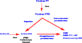
Figure 13.1:
The Initial Integrated FortranD Environment
We can illustrate the portability issues with two anecdotes from
C P. Our original (Cosmic Cube
and Mark II)
hypercubes did not allow the overlap of communication and calculation.
However, we carefully designed the Mark IIIfp to allow the performance
enhancement offered by this overlap. However, we made little use of
this hardware feature because all our codes, algorithms and software
support (CrOS) had been developed for the original hardware. Even the
``Marine Corps'' of C
P. Our original (Cosmic Cube
and Mark II)
hypercubes did not allow the overlap of communication and calculation.
However, we carefully designed the Mark IIIfp to allow the performance
enhancement offered by this overlap. However, we made little use of
this hardware feature because all our codes, algorithms and software
support (CrOS) had been developed for the original hardware. Even the
``Marine Corps'' of C P was not willing to recode applications and
systems software to gain the extra performance. Our software did port
between MIMD machines as they evolved and in this sense message passing
is portable. However, the ``optimal'' message-passing implementation
is hardware dependent and nonportable. The goal of higher level
software systems is to rely on compilers
and runtime
systems to provide such optimization. As a second anecdote, we note
that C
P was not willing to recode applications and
systems software to gain the extra performance. Our software did port
between MIMD machines as they evolved and in this sense message passing
is portable. However, the ``optimal'' message-passing implementation
is hardware dependent and nonportable. The goal of higher level
software systems is to rely on compilers
and runtime
systems to provide such optimization. As a second anecdote, we note
that C P shared a
  CM-2 with Argonne National
Laboratory. C
CM-2 with Argonne National
Laboratory. C P's use of this was disappointing even though several
of our applications, such as QCD in Chapter
4
, were very
suitable for this SIMD architecture. We had excellent parallel (QCD)
codes, which we ran in production, but these were written with message
passing and this could not run on the CM-2. We were not willing to
recode in CMFortran to use the SIMD machine for this problem.
P's use of this was disappointing even though several
of our applications, such as QCD in Chapter
4
, were very
suitable for this SIMD architecture. We had excellent parallel (QCD)
codes, which we ran in production, but these were written with message
passing and this could not run on the CM-2. We were not willing to
recode in CMFortran to use the SIMD machine for this problem.
C P was correct to concentrate on message passing on its MIMD
machines; this is the only way to good performance on most
(excepting the CM-5) MIMD machines even in 1992-ten years after we
started. However, the enduring lesson of C
P was correct to concentrate on message passing on its MIMD
machines; this is the only way to good performance on most
(excepting the CM-5) MIMD machines even in 1992-ten years after we
started. However, the enduring lesson of C P was that ``Parallel
Computing Works.'' There is no reason that our particular software
approach should endure in the same fashion. Rather, we wish to embody
the lessons of C
P was that ``Parallel
Computing Works.'' There is no reason that our particular software
approach should endure in the same fashion. Rather, we wish to embody
the lessons of C P's work into better and higher level software
systems.
P's work into better and higher level software
systems.
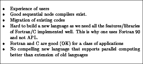
Table 13.1:
Reasons to build parallel languages on top of existing
languages-especially Fortran, C, C++
In 1987, Fox and Kennedy shared a crowded Olympus Airways flight from
Athens to New York. Their conversations were key in establishing the
collaboration on FortranD
[Bozkus:93a;93b], [Choudhary:92c;92d;92e],
[
Fox:91e
], [
Ponnusamy:92c
]. This combined the parallel
compiler expertise of Kennedy [
Callahan:88e
], [Hiranandani:91a;91b],
with C P's wisdom in
practical use of parallel machines. Again, Fox's move to Syracuse
allowed him to compare the successes of CMFortran
on
the SIMD CM-2 with those of message passing on the C
P's wisdom in
practical use of parallel machines. Again, Fox's move to Syracuse
allowed him to compare the successes of CMFortran
on
the SIMD CM-2 with those of message passing on the C P MIMD
emporium. He concluded that one could use high-level data-parallel
Fortran for both SIMD and MIMD machines. This evolved FortranD from
its initial Fortran 77D implementation to include a Fortran 90D version
[
Wu:92a
], illustrated in Figure
13.1
.
Section
13.3
describes some of the experiments leading to this
realization. We will not describe data-parallel Fortran in detail
because the situation is still quite fluid and this is an area that has
grown spectacularly since 1990 when C
P MIMD
emporium. He concluded that one could use high-level data-parallel
Fortran for both SIMD and MIMD machines. This evolved FortranD from
its initial Fortran 77D implementation to include a Fortran 90D version
[
Wu:92a
], illustrated in Figure
13.1
.
Section
13.3
describes some of the experiments leading to this
realization. We will not describe data-parallel Fortran in detail
because the situation is still quite fluid and this is an area that has
grown spectacularly since 1990 when C P finished its project.
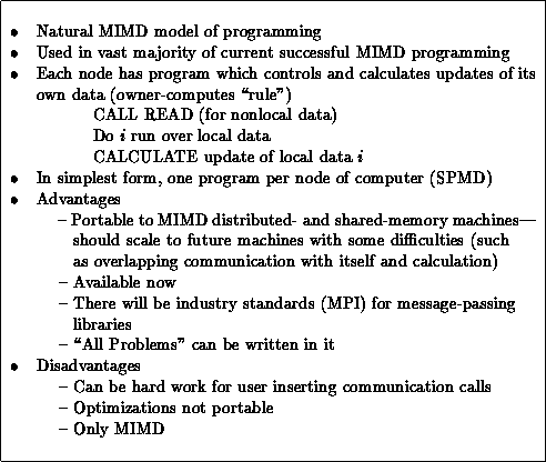
Table 13.2:
Features of the Fortran(C) Plus Message-Passing Paradigm
Section
13.2
describes a prototype software tool built at
Caltech and Rice by Vas Balasundaram and Uli Kremer to enable users to
experiment with different decompositions. This was a component of the
FortranD project set up as part of the NSF Center for Research in
Parallel Computation (CRPC). FortranD was set up as a scalable
language, that is,
``We may need to rewrite our code for a parallel machine, but the
resulting scalable (FortranD) code should run with high efficiency on
`all' current and future anticipated machines.''
Many new parallel languages have been proposed-OCCAM
is
a well known example [
Pritchard:91a
]-but none are ``compelling''
that is, they do not solve enough parallel issues to warrant adoption.
Thus, the recent trend has been to adapt existing languages such as
Fortran [
Brandes:92a
], [
Callahan:88e
], [
Chapman:92a
],
[
Chen:92b
], [
Gerndt:90a
], [
Merlin:92a
], [
Zima:88a
],
C++ [
Bodin:91a
], C [
Hamel:92a
],
[Hatcher:91a;91b], and Lisp. The latter is
illustrated by the successful *Lisp, parallel Lisp implementation
available on the CM-1, 2, and 5. Table
13.1
summarizes some
of the issues involved in choosing to adopt a new language rather than
modifying an old one. Table
13.2
summarizes the
message-passing approach and why we might choose to replace it by a
higher level system, such as data-parallel C or Fortran as summarized
in Table
13.3
. We were impressed by the C language
offered on the CM-2; Section
13.6
describes an early experiment
to develop a loosely synchronous version of this. We should probably
have explored this more thoroughly, although at the time we did not
perceive this as our mission and realized this project would require
major resources to develop a system with good performance. Indeed, the
performance of the early CM-2 C
language
offered on the CM-2; Section
13.6
describes an early experiment
to develop a loosely synchronous version of this. We should probably
have explored this more thoroughly, although at the time we did not
perceive this as our mission and realized this project would require
major resources to develop a system with good performance. Indeed, the
performance of the early CM-2 C compiler was poor and this also
discouraged us. Quinn and Hatcher implemented a similar but more
restrictive C
compiler was poor and this also
discouraged us. Quinn and Hatcher implemented a similar but more
restrictive C MIMD compiler [
Hatcher:91a
]. ASPAR, in
Section
13.5
, had similar goals to Fortran 77D, although it was
targeted more as a migration tool than an efficient complete compiler.
MIMD compiler [
Hatcher:91a
]. ASPAR, in
Section
13.5
, had similar goals to Fortran 77D, although it was
targeted more as a migration tool than an efficient complete compiler.
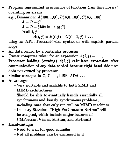
Table 13.3:
Issues in Data-Parallel Fortran Programming Paradigm
FortranD extends Fortran with a set of directives [
Fox:91e
], which
help the compiler produce good code on a parallel machine. These
directives include those specifying the decomposition of the data-parallel
arrays onto the target hardware. The language includes forms of
parallel loop (
Forall
and
DO independent
) for which
parallelization can be asserted without a difficult dependence
analysis. The run time library implements optimized parallel functions
operating on the data-parallel arrays. Fortran 90D also includes the
parallelism implied by the explicit array notation, for example, if
A
,
B
, and
C
are arrays of the same size,
A=B+C
is executed in
parallel. This CRPC research was based in important ways on the
research of C P. Further during 1992, an informal forum
representing all the major players in the parallel computing arena
agreed on a new industry-standard language,
High Performance
Fortran
or HPF
[
Kennedy:93a
]. This embodies all the essential ideas of
FortranD-including the full Fortran 90 syntax. We have modified
FortranD so that HPF is a subset of FortranD. The CRPC FortranD
project continues as a research compiler to investigate extensions of
HPF to handle more general problems and unsolved issues such as
parallel I/O
[
Bordawekar:93a
], [
Rosario:93a
]. We
expect that data-parallel languages should be able to eventually
express nearly all loosely synchronous problems, that is, the vast
majority of scientific and engineering computations.
P. Further during 1992, an informal forum
representing all the major players in the parallel computing arena
agreed on a new industry-standard language,
High Performance
Fortran
or HPF
[
Kennedy:93a
]. This embodies all the essential ideas of
FortranD-including the full Fortran 90 syntax. We have modified
FortranD so that HPF is a subset of FortranD. The CRPC FortranD
project continues as a research compiler to investigate extensions of
HPF to handle more general problems and unsolved issues such as
parallel I/O
[
Bordawekar:93a
], [
Rosario:93a
]. We
expect that data-parallel languages should be able to eventually
express nearly all loosely synchronous problems, that is, the vast
majority of scientific and engineering computations.
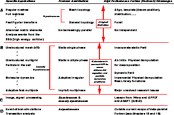
Table 13.4:
High Performance Fortran (HPF) and its extensions
The scope of HPF and FortranD is summarized in Table
13.4
.
Table
13.4
(a) roughly covers both the synchronous and
embarrassingly parallel calculations of Chapters
4
,
6
,
7
, and
8
. Note that we include
computations such as the Kuppermann and McKoy chemical reaction
problems in Chapter
8
, which mix the synchronous and
embarrassingly parallel classes. The original FortranD [
Fox:91e
]
and the initial HPF language [
Kennedy:93a
] should be able to express
these two problem classes in such a way that the compiler will get
good performance on MIMD and, for synchronous problems, SIMD machines
[Choudhary:92d;92e].
Table
13.4
(b) covers the loosely synchronous problems of
Chapters
9
and
12
, which need HPF extensions
to express the irregular structure. We intend to incorporate the
ideas of PARTI [
Berryman:91a
], [
Saltz:91b
] into FortranD as
a prototype of an extended HPF that could handle loosely synchronous
problems. The difficult applications in Sections
12.4
,
12.5
,
12.7
, and
12.8
have a hierarchical tree
structure that is not easy to express [
Bhatt:92a
],
[
Blelloch:92a
], [
Mou:90a
], [
Singh:92a
].
Table
13.4
(c) indicates that we have not yet studied HPF and
FortranD for signal processing applications, although the iWarp group
at Carnegie Mellon University has developed high level languages APPLY
and ADAPT for this problem class [
Webb:92a
]. Table
13.4
(d)
notes that we cannot express in FortranD and HPF the difficult
asynchronous applications introduced in Chapter
14
.
We expect this study and implementation of data-parallel languages to
be a growing and critical area of parallel computing.
In Section
13.7
, we contrast hierarchical and distributed
memory systems. Both require data locality and we expect that data
parallel languages such as High Performance Fortran will be able to
use the HPF directives to improve performance of sequential machines
by exploiting the cache and other levels of memory hierarchy better.
Next:
Problem Architecture and
Up:
13.1 High-Level Languages
Previous:
13.1 High-Level Languages
Guy Robinson
Wed Mar 1 10:19:35 EST 1995
Problem Architecture and Message-Passing Fortran
Next:
13.1.3 Problem Architecture and
Up:
13.1 High-Level Languages
Previous:
13.1.1 High Performance Fortran
Here we discuss the trade off between message-passing and data-parallel
languages
from the problem architecture
point of view developed in Chapter
3
.
We return to Figure
3.4
, which expressed computation as
a sequence of maps. We elaborate this in Figure
13.2
,
concentrating on the map of the (numerical formulation of the) problem
 onto the computer
  . This map could be
performed in several stages reflecting the different software levels.
Here, we are interested in the high-level software map
. This map could be
performed in several stages reflecting the different software levels.
Here, we are interested in the high-level software map  . One often refers to
  as the
virtual machine
(VM), since one can think of it
as abstracting the specific real machine into a generic VM. One could
perhaps more accurately consider it as a virtual problem, since one is
expressing the details of a particular problem in the language of a
general problem of a certain class. Naively, one can say in
Figure
13.2
that
as the
virtual machine
(VM), since one can think of it
as abstracting the specific real machine into a generic VM. One could
perhaps more accurately consider it as a virtual problem, since one is
expressing the details of a particular problem in the language of a
general problem of a certain class. Naively, one can say in
Figure
13.2
that  is ``nearer'' the problem
than the computer. One often thought of CMFortran as a language for
SIMD machines. This is not accurate-rather, it is a language for
synchronous problems (i.e., a particular problem architecture) which
can be executed on all machine architectures. This is illustrated by
the use of CMFortran on the MIMD CM-5 and the HPF (FortranD) discussion
of the previous subsection. These issues are summarized in
Table
13.5
. Generally, we believe that high-level software
systems should be based on a study of problems and their architectures
rather than on machine characteristics.
is ``nearer'' the problem
than the computer. One often thought of CMFortran as a language for
SIMD machines. This is not accurate-rather, it is a language for
synchronous problems (i.e., a particular problem architecture) which
can be executed on all machine architectures. This is illustrated by
the use of CMFortran on the MIMD CM-5 and the HPF (FortranD) discussion
of the previous subsection. These issues are summarized in
Table
13.5
. Generally, we believe that high-level software
systems should be based on a study of problems and their architectures
rather than on machine characteristics.
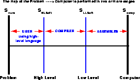
Figure 13.2:
Architecture of ``Virtual Problem'' Determines Nature of
High-Level Language
Figure 13.3 (Color Plate) illustrates the map of problem onto machine,
emphasizing the different architectures of both. Here we regard
message passing as a (low-level  ) paradigm that is
naturally associated with a particular machine architecture, that is, it
does reflect a virtual
machine-the generic
MIMD architecture. One has a trade off in languages between features
optimized for a particular problem class against those optimized for
particular machine architectures. This figure is also drawn so as to
emphasize that HPF corresponds to a
) paradigm that is
naturally associated with a particular machine architecture, that is, it
does reflect a virtual
machine-the generic
MIMD architecture. One has a trade off in languages between features
optimized for a particular problem class against those optimized for
particular machine architectures. This figure is also drawn so as to
emphasize that HPF corresponds to a  ``near'' the
problem and Fortran-plus message passing is a paradigm ``near'' the
computer.
``near'' the
problem and Fortran-plus message passing is a paradigm ``near'' the
computer.
Figure 13.3:
Problem architectures mapped into machine
architectures.
Figure 13.4 (Color Plate) illustrates the compilation and migration
processes from this point of view. HPF is a language that reflects
the problem structure. It is difficult but possible to produce a
compiler that maps it onto the two machine (SIMD and MIMD)
architectures in the figure. Fortran-plus message passing expresses
the MIMD computer architecture. It is typically harder for the user
to express the problem in this paradigm than in the higher level HPF.
However, it is quite easy for the operating system to map explicit
message passing efficiently onto a MIMD architecture. However, this
is not true if one wishes to map message passing to a different
architecture (such as a SIMD machine) where one must essentially
convert (``compile'') the message passing back to the HPF
expression of the problem. This
is typically impossible as the message-passing formulation does not
have all the necessary information contained in it. Expressing a
problem in a specific language often ``hides'' information about the
problem that is essential for parallelization. This is why much of the
existing Fortran 77 sequential code cannot be parallelized. Critical
information about the underlying problem cannot be discovered except at
run time when it is hard to exploit. We discuss this point in more
detail in the following subsection.
Figure 13.4:
migration and compilation in the map of
problems to computers.
Table 13.5:
Message Passing, Data-Parallel Fortran, Problem
Architectures
Next:
13.1.3 Problem Architecture and
Up:
13.1 High-Level Languages
Previous:
13.1.1 High Performance Fortran
Guy Robinson
Wed Mar 1 10:19:35 EST 1995
13.1.3 Problem Architecture and Fortran 77
Next:
A Software Tool
Up:
13.1 High-Level Languages
Previous:
Problem Architecture and
In Section
3.3
, we noted that the concept of space and time
are not preserved in the mappings between complex systems
defined in Equation
3.1
. We can use this to motivate
some advantage in using the array notation used in Fortran 90. Consider a
complex problem whose data domain is expressed in two Fortran arrays
A
and
B
with, say,

Suppose some part of the program involves adding the arrays, which is
expressed as

in Fortran 90 and
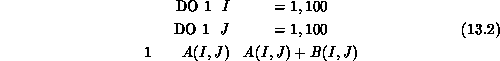
in Fortran 77. In this last equation, the data-parallel spatial
manipulation of Equation
13.1
is converted into 10,000 time
steps. In other words, Fortran 77 has not preserved the spatial
structure of the problem. The task of a parallelizing Fortran 77
compiler is to reverse this procedure by recognizing that the sequential
(time-stepped) DO loops are ``just'' a spatially (data)-parallel
expression. We find mappings:


Note that the final parallel computer implementation maps the original
spatial structure into a combination of time (the ``node'' program)
and space (distribution) over nodes.
We can attribute some of the difficulties in producing an effective
Fortran 77 compiler to the unfortunate mapping of space into time
(control) shown in Equation
13.4
. In the trivial example of
Equation
13.3
, one can undo this ``wrong,'' but in general
there is not enough compile time information in a Fortran 77 code to
recover the original spatial parallelism. In this language,
Fortran-plus message passing also does not preserve the spatial
structure,
but rather maps into a mix of space
(the message-passing parallelism) and time (node Fortran).
Guy Robinson
Wed Mar 1 10:19:35 EST 1995
A Software Tool for Data Partitioning and
Distribution
Next:
13.2.1 Is Any Assistance
Up:
13 Data Parallel C
Previous:
13.1.3 Problem Architecture and
Programming a distributed-memory parallel computer is a complicated
task. It involves two basic steps: (1) specifying the partitioning
of the data, and (2) writing the communication that is necessary in
order to preserve the correct data flow and computation order. The
former requires some intellectual effort, while the latter is
straightforward but tedious work.
We have observed that programmers use several well-known tricks to optimize
the communication in their programs. Many of these techniques are purely
mechanical, relying more on clever juxtapositions and transformations of the
code rather than on a deep knowledge of the algorithm. This is not
surprising, since once the data domain has been partitioned, the data
dependences in the program completely define the communication necessary
between the separate partitions. It should, therefore, be possible for a
software tool to automate step (2), once step (1) has been accomplished by
the programmer.
This would allow the program to be written in a traditional sequential
language extended with annotations for specifying data distribution,
and have a software tool or compiler
mechanically
generate the node program for the distributed-memory computer. This
strategy, illustrated by stages II and III in Figure
13.5
,
is being studied by several researchers [
Callahan:88d
], [
Chen:88b
],
[Koelbel:87a;90a],
[
Rogers:89b
], [
Zima:88a
].
Figure 13.5:
The Program Development Process
What is missing in this scheme? Although the tedious step has been
automated, the hard intellectual step of partitioning the data domain
is still left entirely to the programmer. The choice of a partitioning
strategy often involves some deeper knowledge of the algorithm itself, so we
clearly cannot hope to automate this process completely. We could, however,
provide some assistance in the data partitioning process, so that the
programmer can make a better choice of partitioning schemes from all the
available options. This section describes the design of an interactive data
partitioning tool that provides exactly this kind of assistance.
Next:
13.2.1 Is Any Assistance
Up:
13 Data Parallel C
Previous:
13.1.3 Problem Architecture and
Guy Robinson
Wed Mar 1 10:19:35 EST 1995
13.2.1 Is Any Assistance Really Needed?
Next:
13.2.2 Overview of the
Up:
A Software Tool
Previous:
A Software Tool
The ultimate goal of the programmer is peak performance on the
target computer. The realization of peak performance requires the
understanding of many subtle relationships between the algorithm,
the program, and the target machine architecture. Factors such as input
data size, data dependences in the code, target machine characteristics,
and the data partitioning scheme are related in very nonintuitive
ways, and jointly determine the performance of the program.
Thus, a data partitioning scheme that is chosen purely on the basis
of some algorithmic property, may not always be the best choice.
Let us examine the relationship between these aspects more closely, to
illustrate the subtle complexities that are involved in choosing the
partitioning of the data domain. Consider the following program:\
MMMMMMMMMMMMMMMMMMMMMMMMMM¯example (A, B, N)
double precision A(N, N), B(N, N)
*
do k=1, cycles
do j=1,N
do i=2,N-1
A(i, j) =  ( B(i-1, j), B(i+1, j) )
enddo
enddo
do j=2,N-1
do i=2,N-1
B(i,j) =  ( A(i-1, j), A(i+1, j), A(i, j),
A(i, j-1), A(i, j+1) )
enddo
enddo
enddo
end
 and
and  represent functions with 4 and 10 double-precision
floating-point operations, respectively. This program segment does not
represent any particular realistic computation; rather, it was
chosen to illustrate all the aspects of our argument using a small
piece of code. The program segment was executed on 64 processors of an
nCUBE,
with array sizes ranging from
N = 64
to
N =
320
. A and B were first partitioned as columns, so that each
processor was assigned
represent functions with 4 and 10 double-precision
floating-point operations, respectively. This program segment does not
represent any particular realistic computation; rather, it was
chosen to illustrate all the aspects of our argument using a small
piece of code. The program segment was executed on 64 processors of an
nCUBE,
with array sizes ranging from
N = 64
to
N =
320
. A and B were first partitioned as columns, so that each
processor was assigned  successive columns. The program was then
run once again, this time with A and B partitioned as blocks, so that
each processor was assigned a block of
successive columns. The program was then
run once again, this time with A and B partitioned as blocks, so that
each processor was assigned a block of  elements. The
resulting execution and communication times for column and block
partitioning schemes are shown in Figure
13.6
. The
communication time was measured by removing all computation in the
loops.
elements. The
resulting execution and communication times for column and block
partitioning schemes are shown in Figure
13.6
. The
communication time was measured by removing all computation in the
loops.
Figure 13.6:
Timing results on an nCUBE, using 64 processors.
When employing a column partitioning scheme for arrays A and B, communication
is only necessary after the first
j
loop. Each processor has to
exchange boundary values with its left and right neighbor. In a block
partitioning scheme, each processor has to communicate with its four neighbors
after the first loop and with its north and south neighbors after the second
loop. For small message lengths, the communication cost is dominated
by the message startup time, whereas the transmission cost begins to dominate
as the messages get longer (i.e., more data is exchanged at each
communication step). This explains why communication cost for the column
partition is greater than for the block partition for array sizes larger than
 . It is clear from the graph that column partitioning is
preferable when the array sizes are less than
. It is clear from the graph that column partitioning is
preferable when the array sizes are less than  , and block
partitioning is preferable for larger sizes.
, and block
partitioning is preferable for larger sizes.
The steps in the execution time graphs are caused mainly by load imbalance
effects. For example, the step between
N = 128
and
N = 129
for the column
partition is due to the fact that for size 129 one subdomain has an
extra column, so that the processor assigned to that subdomain is still busy
after all the others have finished, causing load imbalance in the system.
Similar behavior can be observed for the block partition, but here the steps
occur at smaller increments of the array size
N
. The steps in the
communication time graphs are due to the fact that the packet size on the
nCUBE is  , so that messages that are even a few bytes
longer need an extra packet to be transmitted.
, so that messages that are even a few bytes
longer need an extra packet to be transmitted.
The above example indicates that several factors contribute to the observed
performance of a chosen partitioning scheme, making it difficult for a human
to predict this behavior statically. Our aim is to make the programmer aware
of these performance effects without having to run the program on the target
computer. We hope to do this by providing an interactive tool, that can give
performance estimates in response to a data layout specification. The tool's
performance estimates will allow the programmer to gauge the effect of a data
partitioning scheme and thus provide some guidance in making a better choice.
Next:
13.2.2 Overview of the
Up:
A Software Tool
Previous:
A Software Tool
Guy Robinson
Wed Mar 1 10:19:35 EST 1995
13.2.2 Overview of the Tool
Next:
13.2.3 Dependence-based Data Partitioning
Up:
A Software Tool
Previous:
13.2.1 Is Any Assistance
When using the tool we envision, the programmer will select a program
segment for analysis, and the system will provide assistance in choosing an
efficient data partitioning for the computation in that program
segment, for various problem sizes. In a first step, the user
determines a set of reasonable partitionings based on the data
dependence
information and interprocedural
analysis information provided by the tool. An important component of
the system is the performance estimation module, which is subsequently
used to select the best partitionings and distributions from among
those examined. In the present version, the
do
loop is the only
kind of program segment that can be selected. For simplicity, the set
of possible partitions of an array is restricted to regular rectangular
patterns such as by row, by column, or by block for a two-dimensional
array and their higher dimensional analogs for arrays of larger
dimensions. This permits the examination of all reasonable
partitionings of the data in an acceptable amount of time.
The tool will permit the user to generalize from local partitionings to
layouts for an entire program in easy steps, using repartitioning and
redistribution whenever it leads to a better performance overall. In
addition, the tool will support many program transformations that can lead to
more efficient data layouts.
The principal value of such an environment for data partitioning and
distribution is that it supports an exploratory programming style in which
the user can experiment with different data partitioning strategies, and
estimate the effect of each strategy for different input data sizes or
different target machines without having to change the program or run the
program each time.
Guy Robinson
Wed Mar 1 10:19:35 EST 1995
13.2.3 Dependence-based Data Partitioning
Next:
13.2.4 Mapping Data to
Up:
A Software Tool
Previous:
13.2.2 Overview of the
Given a sequential Fortran program and a selected program segment
(which in the preliminary version can only be a loop nest), the tool
provides assistance in deriving a set of reasonable data partitions for
the arrays accessed in that segment. The assistance is given in the
form of data dependence information for variables accessed within the
selected segment. When partitioning data, we must ensure that the
parallel computations done by all the processors on their local
partitions preserve the data dependence relations in the sequential
program segment. If the computations done by the processors on the
distributed data satisfy all the data dependences, the results of the
computation will be the same as those produced by a sequential
execution of the original program segment. There are two ways to
achieve this: (1) by ``internalizing'' data dependences within each
partition, so that all values required by computations local to a
processor are available in its local data subdomain; or (2) by
inserting appropriate communication to get the nonlocal data.
Let us consider a sample program segment and see how data dependence
information can be used to help derive reasonable data partitionings
for the arrays accessed in the segment.
MMMMMMMMMMMMMMMMMMMMMMMMMM¯
P1. Example program segment.
*
do j = 1, n
do i = 1, n
A(i, j) =  ( A(i-1, j) )
B(i, j) =  ( A(i, j), B(i, j-1), B(i, j) )
enddo
enddo
 and
and  represent arbitrary functions, and their exact
nature is irrelevant to this discussion. When the programmer selects the
``
do i
'' loop, the tool indicates that there is one data dependence
that is carried by the
i
loop: the dependence of
represent arbitrary functions, and their exact
nature is irrelevant to this discussion. When the programmer selects the
``
do i
'' loop, the tool indicates that there is one data dependence
that is carried by the
i
loop: the dependence of  on
on
 . This dependence indicates that the computation of
an element of A cannot be started until the element immediately above
it in the previous row has been computed. The programmer then selects the
outer ``
do j
'' loop to get the data dependences that are carried by the
j
loop. There is one such dependence, that of
. This dependence indicates that the computation of
an element of A cannot be started until the element immediately above
it in the previous row has been computed. The programmer then selects the
outer ``
do j
'' loop to get the data dependences that are carried by the
j
loop. There is one such dependence, that of  on
on
 . This dependence indicates that the computation of an
element of B cannot be started until the computation of the element
immediately to the left of it in the previous column has been computed.
Figure
13.7
(a) illustrates the pattern of data dependences for the
above program segment.
. This dependence indicates that the computation of an
element of B cannot be started until the computation of the element
immediately to the left of it in the previous column has been computed.
Figure
13.7
(a) illustrates the pattern of data dependences for the
above program segment.
Figure 13.7:
Data Dependences Satisfied by Internalization and Communication
for the Partitioning Schemes (a) A by Column, B by Column (b) A by Column,
B by Row and (c) A by Block, B by Block. Dotted lines represent partition
boundaries and numbers indicate virtual processor ids (the figures are shown
for
p = 4
virtual processors). For clarity, only a few of the dependences
are shown.
The pattern of data dependences between references to elements of an array
gives the programmer clues about how to partition the array. It is usually a
good strategy to partition an array in a manner that internalizes all data
dependences within each partition, so that there is no need to move data
between the different partitions that are stored on different processors.
This avoids expensive communication via messages. For example, the data
dependence of  on
on  can be satisfied by
partitioning A in a columnwise manner, so that the dependences are
``internalized'' within each partition. The data dependence of
can be satisfied by
partitioning A in a columnwise manner, so that the dependences are
``internalized'' within each partition. The data dependence of
 on
on  can be satisfied by partitioning B
row-wise, since this would internalize the dependences within each partition.
can be satisfied by partitioning B
row-wise, since this would internalize the dependences within each partition.
It is not enough to examine only the dependences that arise due to
references to the same array. In some cases, the data flow in the program
implicitly couples two different arrays together, so that the partitioning
of one affects the partitioning of the other. In our example, each point
 also requires the value
  . We treat this as a
special data dependence (3) called a
value
dependence (read ``B is
value dependent on A''), to distinguish it from the traditional data
dependence that is defined only between references to the same array. This
value dependence must also be satisfied either by internalization or by
communication. Internalization of the value dependence is possible only by
partitioning B in the same manner as A, so that each
. We treat this as a
special data dependence (3) called a
value
dependence (read ``B is
value dependent on A''), to distinguish it from the traditional data
dependence that is defined only between references to the same array. This
value dependence must also be satisfied either by internalization or by
communication. Internalization of the value dependence is possible only by
partitioning B in the same manner as A, so that each  and
the
and
the  value required by it are in the same partition.
Based on the pattern of data dependences in the program segment, the
following are a possible list of partitioning choices that can be
derived:\
-
Partition A by column and B by column. This satisfies the dependences within
A and the value dependences of B on A by internalization but communication is
required to satisfy the data dependences within B (Figure
13.7
(a)).
An analogous case is to partition both A and B by row. This would require
communication to satisfy dependences within A.
-
Partition A by column and B by row. Dependences within B are now satisfied by
internalization, but communication is needed to satisfy the value dependence
of B on A (Figure
13.7
(b)).
-
Partition both A and B as two-dimensional blocks. This would result in
communication to satisfy dependences within both A and B, while the value
dependence of B on A is satisfied by internalization
(Figure
13.7
(c)).
The partitioning of A by row and B by column was not considered among the
possible choices because, in this scheme, none of the dependences are
internalized, thus requiring greater communication compared to (1), (2) or
(3). Communication overhead is a major cause of performance degradation
on most machines, so a reasonable first choice would be the partitioning
scheme that requires the least communication. This can be determined either
by analyzing the number of dependences that are cut by the partitioning
(indicating the need for communication), or more accurately using the
performance estimation module that is described in the next section.
Next:
13.2.4 Mapping Data to
Up:
A Software Tool
Previous:
13.2.2 Overview of the
Guy Robinson
Wed Mar 1 10:19:35 EST 1995
13.2.4 Mapping Data to Processors
Next:
Communication Analysis and
Up:
A Software Tool
Previous:
13.2.3 Dependence-based Data Partitioning
For the selected program segment, the programmer picks one of the
choices (1) through (3), and specifies the data partitioning via an
interface provided by the tool. The tool responds by creating an
internal data mapping that specifies the mapping of the data to a set
of virtual processors. The number of virtual processors is equal to
the number of partitions indicated by the data partitioning. The
mapping of the virtual processors onto the physical processors is
assumed to be done by the run time system, and this mapping is
unspecified in the software layer. Henceforth, we will use the term
``processor'' synonymously with ``virtual processor.'' The internal
data mapping is used by the performance estimator to compute an
estimate of communication and other costs for the program segment. It
is also used by the tool to determine the data that needs to be
communicated between the processors.
Let us continue with our example program segment, and see how the
internal mapping is constructed for partitioning (2), that is, A
partitioned by column and B by row. The data mappings for the other
two cases can be constructed in a similar manner. Let A and B be of size
 and the number of (virtual) processors be
p
. For simplicity we
assume that
p
divides
n
. The following two data mappings are
computed:\
and the number of (virtual) processors be
p
. For simplicity we
assume that
p
divides
n
. The following two data mappings are
computed:\
-
 partitioned by column: Create a virtual array
 , where
  represents the
k
th column partition
of A, that is, A$ consists of the elements
represents the
k
th column partition
of A, that is, A$ consists of the elements  .
The virtual array is only an internal entity, used within the tool to
maintain the mapping of data to (virtual) processors. It does not have any
physical storage on the machine. The partition of A represented by
.
The virtual array is only an internal entity, used within the tool to
maintain the mapping of data to (virtual) processors. It does not have any
physical storage on the machine. The partition of A represented by
 is assumed to be mapped onto the
k
th processor by default.
is assumed to be mapped onto the
k
th processor by default.
-
 partitioned by row: Create a virtual array
 , where
  represents the
i
th row partition of
B, that is, B$ consists of the elements
represents the
i
th row partition of
B, that is, B$ consists of the elements  .
.
 is assigned to the
k
th processor by default.
is assigned to the
k
th processor by default.
The internal data mapping is used to solve the following two
problems:\
-
Given a processor
q
, what part of A is local to it?
This is given by the section of A that belongs to the partition
 .
.
-
Given a section
 , what processors contain
elements of this section? This is given by the set of processors
, what processors contain
elements of this section? This is given by the set of processors
 .
.
The values
n
and
p
are assumed to be known statically.
A useful technique that we will subsequently use on these sections is
called ``translation.'' Translation refers to the conversion of an accessed
section computed with respect to a particular loop to the section accessed
with respect to an enclosing loop. For example, consider a reference
to a two-dimensional array within a doubly nested loop. The section
of the array accessed within each iteration of the innermost loop
is a single element. The same reference, when evaluated with respect to the
entire inner loop (i.e., all iterations of the inner loop) may access a
larger section, such as a column of the array. If we evaluated the reference
with respect to the outer loop (i.e., all iterations of the outer loop), we
may notice that the reference results in an access of the entire array in a
columnwise manner. Translation is thus a method of converting array sections
in terms of enclosing loops, and we will denote this operation
by the symbol `` ''.
''.
The tool uses (1) to determine which processors should do what
computations. The general rule used is: each processor executes only
those program statements whose
l
-values are in its local storage. The
l
-values computed by a processor are said to be
owned
by
the processor. In order to compute an
l
-value, several
r
-values may be
required, and not all of them may be local to that processor. The inverse
mapping (2) is used to determine the set of processors that own the desired
r
-values. These processors must send the
r
-value they own to the
processor that will execute the statement.
The data mapping scheme described above works only for arrays. Scalar
variables are assumed to be replicated, that is, every processor stores a copy
of the scalar variable in its local memory. By the rule stated earlier, this
implies that any statement that computes the value of a scalar is executed by
all the processors.
Next:
Communication Analysis and
Up:
A Software Tool
Previous:
13.2.3 Dependence-based Data Partitioning
Guy Robinson
Wed Mar 1 10:19:35 EST 1995
Communication Analysis and Performance Improvement
Transformations
Next:
13.2.6 Communication Analysis Algorithm
Up:
A Software Tool
Previous:
13.2.4 Mapping Data to
The communication analysis algorithm takes the internal data mappings, the
dependence graph, and the loop nesting structure of the specified program
segment as its input. For each processor the algorithm determines information
about all communications the processor is involved in. We will now
illustrate the communication analysis algorithm using the example program
segments P1, P2, and P3, where P2 is derived from P1, and P3 from P2,
respectively, by a transformation called
loop distribution
.
Substantial performance improvement can be achieved by performing various
code transformations on the program segment. For example, the
loop-distribution
transformation [
Wolfe:89a
] often helps reduce
the overhead of communication. Loop distribution splits a loop into a set of
smaller loops, each containing a part of the body of the original loop.
Sometimes, this allows communication to be done between the resulting loops,
which may be more efficient than doing the communication within the original
loop.
Consider the program segment P1. If A is partitioned by column and B by row,
communication will be required within the inner loop to satisfy the value
dependence of B on A. Each message communicates a single element of A.
For small message sizes and a large number of messages, the fraction of
communication time taken up by message startup overhead is usually quite
large. Thus, program P1 will most likely give poor performance because it
involves the communication of a large number of small messages.
However, if we loop-distributed the inner
do i
loop over the two
statements, the communication of A from the first
do i
loop to the
second
do i
loop can be done between the two new inner loops. This
allows each processor to finish computing its entire column partition of A in
the first
do i
loop, and then send its part of A to the appropriate
processors as larger messages, before starting computation of a partition of
B in the second
do i
loop. This communication is done only once for
each iteration of the outer
do j
loop, that is, a total of O(n)
communication steps. In comparison, program P1 requires communication within
the inner loop, which gives a total of O( ) communication
steps:\
) communication
steps:\
MMMMMMMMMMMMMMMMMMMMMMMMMM¯
P2. After loop distribution of i loop.
*
do j = 2, n
do i = 2, n
A(i, j) =  ( A(i
-
1, j) )
( A(i
-
1, j) )
enddo
do i = 2, n
B(i, j) =  ( A(i, j), B(i, j
-
1), B(i, j) )
( A(i, j), B(i, j
-
1), B(i, j) )
enddo
enddo
The reduction in the number of communication steps also results in greater
parallelism, since the two inner
do i
loops can be executed in parallel
by all processors without any communication. This effect is much more
dramatic if we apply loop distribution once more, this time on the outer
do j
loop:\
MMMMMMMMMMMMMMMMMMMMMMMMMM¯
P3. After loop distribution of j loop.
*
do j = 2, n
do i = 2, n
A(i, j) =  ( A(i
-
1, j) )
( A(i
-
1, j) )
enddo
enddo
do j = 2, n
do i = 2, n
B(i, j) =  ( A(i, j), B(i, j
-
1), B(i, j) )
( A(i, j), B(i, j
-
1), B(i, j) )
enddo
enddo
For the same partitioning scheme (i.e., A by column and B by row), we
now need only O(1) communication steps, which occur between the two outer
do j
loops. The computation of A in the first loop can be done in
parallel by all processors, since all dependences within A are internalized
in the partitions. After that, the required communication is performed to
satisfy the value dependence of B on A. Then the computation of B can proceed
in parallel, because all dependences within B are internalized in the
partitions. The absence of any communication within the loops considerably
improves efficiency.
Currently, the tool provides a menu of several program
transformations,
and the programmer can
choose which one to apply. When a particular transformation is chosen
by the programmer, the tool responds by automatically performing the
transformation on the program segment, and updating all internal
information automatically.
Next:
13.2.6 Communication Analysis Algorithm
Up:
A Software Tool
Previous:
13.2.4 Mapping Data to
Guy Robinson
Wed Mar 1 10:19:35 EST 1995
13.2.6 Communication Analysis Algorithm
Next:
13.2.7 Static Performance Estimator
Up:
A Software Tool
Previous:
Communication Analysis and
For the sake of illustration, let the size of A and B be  (i.e.,
n = 8
), and let the number of (virtual) processors be
p = 4
.
The following is a possible sequence of actions that the programmer could do
using the tool.
(i.e.,
n = 8
), and let the number of (virtual) processors be
p = 4
.
The following is a possible sequence of actions that the programmer could do
using the tool.
After examining the data dependences within the program segment as reported
by the tool, let us assume that the programmer decides to partition A
by column and B by row. The tool computes the internal mapping:\
A$(1) = A(1:8, 1:2) and B$(1) = B(1:2, 1:8).
A$(2) = A(1:8, 3:4) and B$(2) = B(3:4, 1:8).
A$(3) = A(1:8, 5:6) and B$(3) = B(5:6, 1:8).
A$(4) = A(1:8, 7:8) and B$(4) = B(7:8, 1:8).
To determine the communication necessary, the tool uses Algorithm COMM, shown
in Figure
13.8
. For simple partitioning schemes as found in many
applications, the communication computed by algorithm COMM can be
parameterized by processor number, that is, evaluated once for an arbitrary
processor. In addition, we are also investigating other methods to speed up
the algorithm.
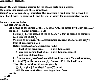
Figure 13.8:
Algorithm to Determine the Communication Induced by the Data
Partitioning Scheme
Consider program P1 for example. According to algorithm COMM, when the
k
th processor executes the first statement, the required communication is
given by

where the range of
i
and
j
are determined by the section of the LHS
owned by processor
k
, in this case  and
and  (since A
is partitioned columnwise). But the partitioning of A ensures that
(since A
is partitioned columnwise). But the partitioning of A ensures that
 , the data
  is always local to
k
. The set of
is always local to
k
. The set of  pairs will, therefore, be an empty set for
any
k
. Thus, the execution of the first statement with A partitioned by
column requires no communication.
pairs will, therefore, be an empty set for
any
k
. Thus, the execution of the first statement with A partitioned by
column requires no communication.
When the
k
th processor executes the second statement, the communication as
computed by algorithm COMM is given by
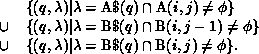
The ranges of
i
and
j
are determined by the section of the LHS that is
owned by processor
k
: in this case  and
and  (since B
is partitioned rowwise). The second and third terms will be
(since B
is partitioned rowwise). The second and third terms will be  ,
because the row partitioning of B ensures that
,
because the row partitioning of B ensures that  , the data
 is always local to
k
. The first term can be
a nonempty set, because processor
k
owns a column of A (i.e.,
j
in
the range
is always local to
k
. The first term can be
a nonempty set, because processor
k
owns a column of A (i.e.,
j
in
the range  ), while the range of
j
in the first term is
), while the range of
j
in the first term is  .
Thus, communication may be required to get the nonlocal element of A before
the
k
th processor can proceed with the computation of its
.
Thus, communication may be required to get the nonlocal element of A before
the
k
th processor can proceed with the computation of its  .
The dependence from the definition of
.
The dependence from the definition of  to its use is
loop-independent. Algorithm COMM therefore computes
commlevel
, the
common nesting level of the source and sink of the dependence, to be the
level of the inner
i
loop. The section
to its use is
loop-independent. Algorithm COMM therefore computes
commlevel
, the
common nesting level of the source and sink of the dependence, to be the
level of the inner
i
loop. The section  translated to the
level of the inner
i
loop is simply the single element
translated to the
level of the inner
i
loop is simply the single element  .
Thus, each message communicates this single element and the communication
occurs within the inner
i
loop.
.
Thus, each message communicates this single element and the communication
occurs within the inner
i
loop.
The execution of program P1 results in a large number of messages because
each message only communicates a single element of A, and the communication
occurs within the inner loop. Message startup and transmission costs are
specified by the target machine parameters, and the average cost of each
message is determined from the performance model. The tool computes the
communication cost by multiplying the number of messages by the average cost
of sending a single element message. This cost estimate is returned to
the programmer.
Now consider the program P2, with the same partitioning scheme for A and B.
When the
k
th processor executes the first statement, the required
communication as determined by algorithm COMM is given by

where the range of
j
is determined by the section of the LHS
owned by processor
k
, in this case 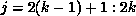 (since A is
partitioned columnwise). Note that in this case,
(since A is
partitioned columnwise). Note that in this case,  . This is because
commlevel
is now the level of the
outer
j
loop, so that the section
. This is because
commlevel
is now the level of the
outer
j
loop, so that the section  must be translated to
the level of the
j
loop. In other words, the reference to
must be translated to
the level of the
j
loop. In other words, the reference to  )
in the first statement results in an access of the first seven elements of
the
j
th column of A, during each iteration of the
j
loop. Since A is
partitioned columnwise, this section will always be available locally in
each processor, so that the above set is empty and no communication is
required.
)
in the first statement results in an access of the first seven elements of
the
j
th column of A, during each iteration of the
j
loop. Since A is
partitioned columnwise, this section will always be available locally in
each processor, so that the above set is empty and no communication is
required.
When processor
k
executes the second statement, the communication required
is given by
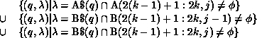
The second and third terms will be empty sets since the required part of B is
local to each
k
(because B is partitioned rowwise). The first term will
be nonempty, because each processor owns  , and
the range of
j
in the first term is outside the range
, and
the range of
j
in the first term is outside the range 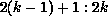 . The
data required by processor
k
from processor
q
will therefore be a strip
. The
data required by processor
k
from processor
q
will therefore be a strip
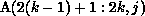 , from each
  .
.
This data can be communicated between the two inner
do i
loops. Each
message will communicate a  size strip of A. Fewer exchanges will
be required compared to program P1, because each exchange now communicates a
strip of A, and the communication occurs outside the inner loop. Once again,
the performance model and target machine parameters are used by the tool to
estimate the total communication cost, and this cost is returned to the
programmer.
size strip of A. Fewer exchanges will
be required compared to program P1, because each exchange now communicates a
strip of A, and the communication occurs outside the inner loop. Once again,
the performance model and target machine parameters are used by the tool to
estimate the total communication cost, and this cost is returned to the
programmer.
For most target machines, the communication cost in program P2 will be
considerably less than in program P1, because of larger message size and
fewer messages.
Next, let us consider program P3. Assuming that the same partitioning scheme
is used for A and B, the execution of the first loop by the
k
th processor
will require communication given by

But this is an empty set because of the column partitioning of A. Here
 , because
commlevel
for this case is the level of the subroutine that contains the two loops.
The section is, therefore, translated to this level by substituting the
appropriate bounds for
i
and
j
. The translated section indicates that the
reference
, because
commlevel
for this case is the level of the subroutine that contains the two loops.
The section is, therefore, translated to this level by substituting the
appropriate bounds for
i
and
j
. The translated section indicates that the
reference  in the first statement results in an access of the
section
in the first statement results in an access of the
section  during all iterations of the outer
j
loop that are executed by processor
k
.
during all iterations of the outer
j
loop that are executed by processor
k
.
When the
k
th virtual processor executes the second loop, the required
communication is
The second and third terms will be empty sets because of the row
partitioning of B. The first term will be nonempty, and the data required by
processor
k
from processor
q
will be the block  ,
,
 , for each
  . This block can be communicated between
the two
do j
loops.
. This block can be communicated between
the two
do j
loops.
This communication can be done between the two loops, allowing computation
within each of the two loops to proceed in parallel. The number of messages
is the fewest for this case because a  block of A is communicated
during each exchange. Program P3 is thus likely to give superior performance
compared to P1 or P2, on most machines. We ran programs P1, P2 and P3 with
A partitioned by column and B by row, on 16 processors of the nCUBE at
Caltech. The functions
block of A is communicated
during each exchange. Program P3 is thus likely to give superior performance
compared to P1 or P2, on most machines. We ran programs P1, P2 and P3 with
A partitioned by column and B by row, on 16 processors of the nCUBE at
Caltech. The functions  and
and  consisted of one and two
double-precision floating-point operations, respectively. The results of the
experiment are shown in Figure
13.9
. The graphs clearly illustrate
the performance improvement that occurs due to reduction in number of
messages and increase in length of each message.
consisted of one and two
double-precision floating-point operations, respectively. The results of the
experiment are shown in Figure
13.9
. The graphs clearly illustrate
the performance improvement that occurs due to reduction in number of
messages and increase in length of each message.
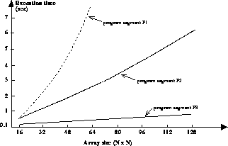
Figure 13.9:
Timing Results for Programs P1, P2 and P3 on the nCUBE, Using 16
Processors.
Next:
13.2.7 Static Performance Estimator
Up:
A Software Tool
Previous:
Communication Analysis and
Guy Robinson
Wed Mar 1 10:19:35 EST 1995
13.2.7 Static Performance Estimator
Next:
13.2.8 Conclusion
Up:
A Software Tool
Previous:
13.2.6 Communication Analysis Algorithm
Given the results of the communication analysis in a program segment,
the performance estimator
can be used to
predict the performance of that program segment on the target machine.
The realization of such an estimator requires a simple static model of
performance that is based on (1) target machine parameters such as the
number of processors, the message startup and transmission costs, and
the average times to perform different floating-point operations; (2)
the size of the input data set; and (3) the data partitioning scheme.
We undertook a study of published performance models [
Chen:88b
],
[
Fox:88a
], [
Gustafson:88a
], [
Saltz:87b
] for use in the
performance estimator, and noticed that these theoretical models did not give
accurate predictions in many cases. We concluded that the theoretical models
suffered from the following deficiencies:\
-
Most of the models suggested in the literature were aimed at being
``general-purpose,'' that is, intended to model the performance of any
distributed-memory MIMD computer. This generality created problems in some
cases, when machine-specific peculiarities tended to skew the observed
results from the ones predicted by the model.
-
The models also did not account for all of the software overhead
involved in implementing the low-level communication utilities on the
machine. While the models accounted for things like message startup costs
and packetizing costs, they often ignored factors such as internal buffer
sizes, peculiarities of the algorithms used to implement the
message passing protocols, and so on.
Our effort to correct these defects resulted in an increased complexity
of the model, and also necessitated the introduction of several
machine-specific features. We felt that this was undesirable, and decided to
investigate alternative methods [
Balasundaram:90d
].
We constructed a program that tested a series of communication patterns
using a set of basic low-level portable communication utilities. This
program, called a ``training set,'' is executed once on the target machine.
The program computes timings for the different communication operations and
averages them over all the processors. These timings are determined for a
sequence of increasing data sizes. Since the graph of communication cost
versus data size is usually a linear function, it can easily be described by
specifying a few parameters (e.g., the slope). The training set
thus generates a table whose entries contain the minimal information
necessary to completely define the performance characteristic for each
communication utility. This table is used in place of the theoretical model
for the purposes of performance prediction.
Figure
13.10
shows some communication cost characteristics created
using a part of our training set on 32 processors of an nCUBE. The data
space was assumed to be a two-dimensional array that was partitioned
columnwise; that is, each processor was assigned a set of consecutive
columns. The communication utilities tested here are:\
-
iSR
: nearest-neighbor individual element send and receive,
using the EXPRESS calls exwrite() and exread().
-
vSR
: nearest-neighbor vector send and receive along one direction,
using the EXPRESS calls exvwrite() and exvread().
-
EXCH1
: nearest-neighbor vector exchange along one
direction, using the EXPRESS call exvchange().
-
vSRSR
: nearest-neighbor vector sends and
receives along two directions,
using the EXPRESS calls exvwrite() and exvread().
-
EXCH2
: nearest-neighbor vector exchange along two
directions, using two calls to exvchange().
-
COMBN
: combine operation over all processors, using
the EXPRESS call excombine().
-
BCAST
: one to all broadcast
, using the
EXPRESS call exbroadcast().
Figure 13.10:
Communication cost characteristics of some EXPRESS utilities on the
nCUBE
The table generated by the training set for the characteristics shown in
Figure
13.10
is:\
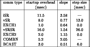
The communication cost estimate for a particular data size is then
calculated using the formula:\

where ``pkt size'' is the size of each message packet, which on the nCUBE
is 1024 bytes ( ).
).
The static performance model is meant primarily to help the programmer
discriminate between different data partitioning schemes. Our approach is to
provide the programmer with the necessary tools to experiment with several
data partitioning strategies, until he can converge on the one that is likely
to give him a satisfactory performance. The tool provides feedback
information about performance estimates each time a partitioning is done by
the programmer.
Next:
13.2.8 Conclusion
Up:
A Software Tool
Previous:
13.2.6 Communication Analysis Algorithm
Guy Robinson
Wed Mar 1 10:19:35 EST 1995
13.2.8 Conclusion
Next:
13.3 Fortran 90 Experiments
Up:
A Software Tool
Previous:
13.2.7 Static Performance Estimator
Our emphasis in this work has been to try to recognize
collective
communication patterns rather than generate sequences of individual element
sends and receives. Algorithm COMM determines this in a very natural way.
This is especially important for loosely synchronous problems which
represent a large class of scientific computations [
Fox:88a
].
Several communication utilities have been developed that provide optimal
message-passing communication for such problems, provided the communication
is of a regular nature and occurs collectively [
Fox:88h
].
We believe that our approach can be extended to derive partitioning schemes
automatically. Data dependence and other information can be used to compute a
fairly restricted set of reasonable data partitioning schemes for a selected
program segment. The performance estimation module can then be applied
in turn to each of the partitionings in the computed set.
The work described in this section was a joint effort between Caltech and
Rice University, as part of the Center for Research on Parallel Computation
(CRPC) research collaboration [
Balasundaram:90a
]. The principal
researchers were Vasanth Balasundaram and Geoffrey Fox at Caltech, and Ken
Kennedy and Ulrich Kremer at Rice. The data partitioning tool described here
is being implemented as part of the ParaScope parallel programming
environment under development at Rice University [
Balasundaram:89c
].
Guy Robinson
Wed Mar 1 10:19:35 EST 1995
13.3 Fortran 90 Experiments
Next:
13.4 Optimizing Compilers by
Up:
13 Data Parallel C
Previous:
13.2.8 Conclusion
Near the end of the C P work at Caltech, we did some important
experiments using Fortran 90 which formed the basis of the aspects of
the FortranD project overviewed in Section
13.1
. These were
partly motivated by Fox's change of architectural environment. At
Caltech, he was surrounded by MIMD machines and the associated
culture; at Syracuse's NPAC facility, the centerpiece in 1990 was a
P work at Caltech, we did some important
experiments using Fortran 90 which formed the basis of the aspects of
the FortranD project overviewed in Section
13.1
. These were
partly motivated by Fox's change of architectural environment. At
Caltech, he was surrounded by MIMD machines and the associated
culture; at Syracuse's NPAC facility, the centerpiece in 1990 was a
 -node SIMD CM-2. In reading the CMFortran (Fortran 90)
manual, Fox noted that the Fortran 90 run time support included all the
important collective communication
primitives (such as combine and broadcast) we had found important in
CrOS and Express.
-node SIMD CM-2. In reading the CMFortran (Fortran 90)
manual, Fox noted that the Fortran 90 run time support included all the
important collective communication
primitives (such as combine and broadcast) we had found important in
CrOS and Express.
The first experiment involved a climate modelling code using spectral
methods [Keppenne:89a;90a]. We had rashly
promised a TRW group that we would be able to easily parallelize such
a code. However, we had not realized that the code was written in C
with extensive C++-like use of pointers. ParaSoft-responsible for
the code conversion-was horrified and the task seemed daunting!
However, Keppenne was interested in rewriting the code in Fortran 90,
which was a ``neat'' language like C++. ParaSoft found that the
resultant Fortran 90 code was straightforward to port to a variety of
parallel machines, as shown in Tables
13.6
and
13.7
. Note that the new version of the code had
an order-of-magnitude-higher performance than the original one on a
single CPU CRAY Y-MP. The discipline implied by Fortran 90 allowed
both ``outside computational scientists'' and the Cray compiler to
``understand'' the code. We analyzed this process and believe that we
could indeed replace our friends at ParaSoft for this problem by a
compiler-initially Fortran 90D-which could generate good
SIMD and MIMD code. This is, of course, the motivation of use of the
array syntax feature in High Performance Fortran as it captures the
parallelism in a transparent fashion.
Table 13.6:
Logistics of Migration Experiment on Climate Code
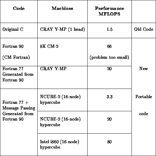
Table 13.7:
Performance of a Climate Modelling Computational Kernel. In
each case, only minor (obviously needed) optimizations were performed.
This experiment motivated the Fortran 90D language [
Fox:91f
],
[
Wu:92a
], and we followed up the climate experiments with some
other simple examples, which are summarized in Table
13.8
.
This compares ``optimal hand-coded'' Fortran-plus message-passing code
with what we expect a good Fortran 90D (HPF) compiler could produce
from the (annotated) Fortran 90
source. The results are essentially perfect for the
Gaussian elimination example and reasonable for the FFT.
These estimates were borne out in practice [Bozkus:93a;93b]
and the prototype Fortran 90D
compiler developed at Syracuse produced code that was about 10% slower
than the optimal node Fortran 77+ message-passing version.
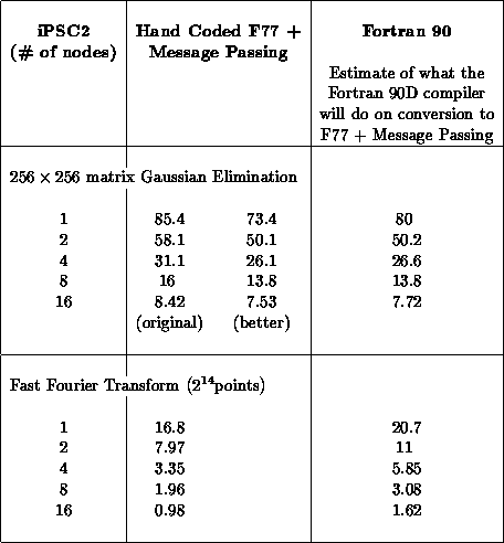
Table 13.8:
Effectiveness of Fortran 90 on Two Simple Kernels. The
execution time is given as a function of the number of nodes used in
the iPSC2 multicomputer.
Next:
13.4 Optimizing Compilers by
Up:
13 Data Parallel C
Previous:
13.2.8 Conclusion
Guy Robinson
Wed Mar 1 10:19:35 EST 1995
13.4 Optimizing Compilers by Neural Networks
Next:
13.5 ASPAR
Up:
13 Data Parallel C
Previous:
13.3 Fortran 90 Experiments
The ability of neural networks
to compute solutions
to optimization problems has been widely appreciated since Hopfield and
Tank's work on the travelling salesman
problem [
Hopfield:85b
]. Chapter
11
reviews the general work
in C P on optimization and physical and neural approaches. We have
examined whether neural network optimization can be usefully applied to
compiler
optimizations. The problem is nontrivial
because compiler optimizations usually involve intricate logical
reasoning, but we were able to find an elegant formalism for turning a
set of logical constraints into a neural network [
Fox:89l
].
However, our conclusions were that the method will only be viable if
and when large hierarchically structured neural networks can be built.
The neural approach to compiler optimization is worth pursuing, because
such a compiler would not be limited to a finite set of code
transformations and could handle unusual code routinely. Also, if the
neural network were implemented in hardware, a processor could perform
the optimizations at run time on small windows of code.
P on optimization and physical and neural approaches. We have
examined whether neural network optimization can be usefully applied to
compiler
optimizations. The problem is nontrivial
because compiler optimizations usually involve intricate logical
reasoning, but we were able to find an elegant formalism for turning a
set of logical constraints into a neural network [
Fox:89l
].
However, our conclusions were that the method will only be viable if
and when large hierarchically structured neural networks can be built.
The neural approach to compiler optimization is worth pursuing, because
such a compiler would not be limited to a finite set of code
transformations and could handle unusual code routinely. Also, if the
neural network were implemented in hardware, a processor could perform
the optimizations at run time on small windows of code.
Figure
13.11
shows how a simple computation of  is
scheduled by a neural network. The machine state is represented at five
consecutive cycles by five sets of 20 neurons. The relevant portion of the
machine comprises the three storage locations
a
,
b
,
c
and a register
r
, and the machine state is defined by showing which of the five quantities
A
,
B
,
C
,
is
scheduled by a neural network. The machine state is represented at five
consecutive cycles by five sets of 20 neurons. The relevant portion of the
machine comprises the three storage locations
a
,
b
,
c
and a register
r
, and the machine state is defined by showing which of the five quantities
A
,
B
,
C
,  and
and  occupies which location. A firing neuron
(i.e., shaded block) in row
occupies which location. A firing neuron
(i.e., shaded block) in row  and column
r
indicates that
and column
r
indicates that  is in
the register. The neural network is set up to ``know'' that computations can
only be done in the register, and it produces a firing pattern representing a
correct computation of
is in
the register. The neural network is set up to ``know'' that computations can
only be done in the register, and it produces a firing pattern representing a
correct computation of  .
.
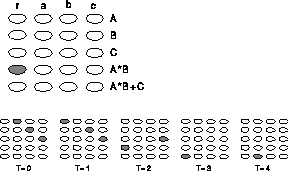
Figure 13.11:
A Neural Network Can Represent Machine States (top) and
Generate Correct Machine Code for Simple Computations (bottom).
The neural compiler was conceived by Geoffrey Fox and investigated
by Jeff Koller [
Koller:88c
],
[Fox:89l;90nn].
Next:
13.5 ASPAR
Up:
13 Data Parallel C
Previous:
13.3 Fortran 90 Experiments
Guy Robinson
Wed Mar 1 10:19:35 EST 1995
13.5 ASPAR
Next:
13.5.1 Degrees of Difficulty
Up:
13 Data Parallel C
Previous:
13.4 Optimizing Compilers by
ASPAR was developed by Ikudome from C P [
Ikudome:90a
] in
collaboration with ParaSoft. It was aimed at aiding the conversion of
existing Fortran codes and embodies the experience especially of
Flower and Kolawa. ASPAR is aimed at those applications involving
particular stencil operation on arrays-noting that many sequential
stencils need modification for parallel execution. In this way, ASPAR
involves a collaboration between user and compiler in the
parallelization process. The discussion in this section is due to
Flower and Kolawa, and we include some of the introductory material as
a contrast to the discussion given in the introductory sections of
each chapter in this book, which largely reflect Fox's prejudice.
P [
Ikudome:90a
] in
collaboration with ParaSoft. It was aimed at aiding the conversion of
existing Fortran codes and embodies the experience especially of
Flower and Kolawa. ASPAR is aimed at those applications involving
particular stencil operation on arrays-noting that many sequential
stencils need modification for parallel execution. In this way, ASPAR
involves a collaboration between user and compiler in the
parallelization process. The discussion in this section is due to
Flower and Kolawa, and we include some of the introductory material as
a contrast to the discussion given in the introductory sections of
each chapter in this book, which largely reflect Fox's prejudice.
It is now a widely accepted fact that parallel computing is a successful
technology. It has been applied to problems in many fields and has achieved
excellent results on projects ranging in scope from academic demonstrations
to complete commercial applications, as shown by other sections of
this book.
Despite this success, however, parallel computing is still considered
something of a ``black art'' to be undertaken only by those with intimate
knowledge of hardware, software, physics, computer science and a wealth of
other complex areas. To the uninitiated there is something frightening about
the strange incantations that abound in parallel processing circles-not
just the ``buzz words'' that come up in polite conversation but the complex
operations carried out on a once elegant piece of sequential code in order
for it to successfully run on a parallel processing system.
Guy Robinson
Wed Mar 1 10:19:35 EST 1995
13.5.1 Degrees of Difficulty
Next:
13.5.2 Various Parallelizing Technologies
Up:
13.5 ASPAR
Previous:
13.5 ASPAR
It is easy to define various ``degrees of difficulty'' in parallel processing.
One such taxonomy might be as follows:
-
Extremely difficult (
Asynchronous
)
In this category fall the complex, asynchronous, real-time
applications. A good example of such a beast is ``parallel
chess''
[
Felten:88h
] of Section
14.3
,
where AI heuristics
must be combined with real-time
constraints to solve the ill-posed problem of searching the ``tree'' of
potential moves.
-
Complex (
Compound Metaproblems
)
In this area one might put the very large applications of fairly
straightforward science. Often, algorithms must be carefully
constructed, but the greatest problems are the large scale of the
overall system and the fact that different ``modules'' must be
integrated into the complete system. An example might be the SDI
simulation ``Sim88'' and its successors [
Meier:90a
] described in
Section
18.3
. The parallel processing issues in such a
code require careful thought but pose no insurmountable problems.
-
Hard (
Loosely Synchronous
)
Problems such as large-scale fluid dynamics or oceanography
[
Keppenne:90b
] mentioned in Section
13.3
often have complex
physics but fairly straightforward and well-known numerical methods.
In these cases, the majority of the work involved in parallelization
comes from analysis of the individual algorithms which can then often
be parallelized separately. Each submodule is then a simpler,
tractable problem which often has a ``well-known'' parallel implementation.
-
Straightforward but Tedious (
Synchronous
)
The simplest class of ``interesting'' parallel programs are partial
differential equations [
Brooks:82b
], [
Fox:88a
] and the
applications of Chapters
4
and
6
. In
these cases the parallel processing issues are essentially trivial but
the successful implementation of the algorithm still requires some care
to get the details correct.
-
Trivial
The last class of problems are those with ``embarrassing parallelism''
such as in Chapter
7
-essentially uncoupled loop
iterations or functional units. In these cases, the parallel processing
issues are again trivial but the code still requires care if it is to
work correctly in all cases.
The ``bottom line'' from this type of analysis is that all but the hardest
cases pose problems in parallelization which are, at least conceptually,
straightforward. Unfortunately, the actual practice of turning such concepts
into working code is never trivial and rarely easy. At best it is usually
an error-prone and time-consuming task.
This is the basic reason for ASPAR's existence. Experience has taught us
that the complexities of parallel processing are really due not to any
inherent problems but to the fact that human beings and parallel computers
don't speak the same language. While a human can usually explain a parallel
algorithm on a piece of paper with great ease, it is often a
significant task to convert that picture to functional code. It is our
hope that the bulk of the work can be automated by the use of
``parallelizing'' technologies such as ASPAR. In particular, we
believe (and our results so far bear out this belief) that problems in
all the previous categories (except possibly (1) above), can be either
completely or significantly automated.
Next:
13.5.2 Various Parallelizing Technologies
Up:
13.5 ASPAR
Previous:
13.5 ASPAR
Guy Robinson
Wed Mar 1 10:19:35 EST 1995
13.5.2 Various Parallelizing Technologies
Next:
13.5.3 The Local View
Up:
13.5 ASPAR
Previous:
13.5.1 Degrees of Difficulty
To understand the issues involved in parallelizing codes and the difference
between ASPAR and other similar tools, we must examine two basic issues
involved in parallelizing code: the local and the global views.
The local view of a piece of code is restricted to one or more loops or
similar constructs upon which particular optimizations are to be applied. In
this case little attention is paid to the larger scale of the application.
The global view of the program is one in which the characteristics of a
particular piece of data or a function are viewed as a part of the complete
algorithm. The impact of operating on one item is then considered in the
context of the entire application. We believe that ASPAR offers a completely
new approach to both views.
Guy Robinson
Wed Mar 1 10:19:35 EST 1995
13.5.3 The Local View
Next:
13.5.4 The ``Global'' View
Up:
13.5 ASPAR
Previous:
13.5.2 Various Parallelizing Technologies
``Local'' optimization is a method which has been used in compilers for many
years and whose principles are well understood. We can see the
evolutionary path to ``parallelizing compilers''
as follows.
-
Vectorizing Compilers
The goal of automatic parallelization is obviously not new, just as parallel
processors are not new. In the past, providing support for advanced
technologies was in the realm of the compiler, which assumed the onus, for
example, of hiding vectorizing hardware from the innocent users.
Performing these tasks typically involves a fairly simple line of thought
shown by the ``flow diagram'' in Figure
13.12
. Basically the
simplest idea is to analyze the dependences between data objects within
loops. If there are no dependences, then ``kick'' the vectorizer into
performing all, or as many as it can handle, of the loop iterations at once.
Classic vector code therefore has the appearance
DO 10 I=1,10000
DO 10 I=1,A(I) = B(I) + C(I)*D(I)
10 CONTINUE
Figure 13.12:
Vectorizability Analysis
-
Parallelizing Compilers
We can easily derive parallelizing compilers from this type of technology by
changing the box marked ``vectorize'' in Figure
13.12
to one
marked ``parallelize.'' After all, if the loop iterations are independent,
parallel operation is straightforward. Even better results can often be
achieved by adding a set of ``restructuring operations'' to the analysis as
shown in Figure
13.13
.
Figure 13.13:
A Parallelizing Compiler
The idea here is to perform complex ``code transformations'' on cases which
fail to be independent during the first dependence analysis in an attempt to
find a version of the same algorithm with fewer dependences. This type of
technique is similar to other compiler optimizations such as
loop unrolling
and
code inlining
[
Zima:88a
], [
Whiteside:88a
]. Its goal is to
create new code which produces exactly the same result when executed but
which allows for better optimization and, in this case, parallelization.
-
ASPAR
The emphasis of the two previous techniques is still on producing exactly the
same result in both sequential and parallel codes. They also rely heavily on
sophisticated compiler technology to reach their goals.
ASPAR takes a rather different approach. One of its first assumptions is
that it may be okay for the sequential and parallel codes to give different
answers!
In technical terms, this assumption removes the requirement that loop
iterations be independent before parallelization can occur. In practical
terms, we can best understand this issue by considering a simple example:
image analysis.
One of the fundamental operations of image analysis is ``convolution.''
The basic idea is to take an image and replace
each pixel value by an average of its neighbors. In the simplest case
we end up with an algorithm that looks like
DO 10 I = 2,N-1
DO 20 J = 2,N-1
DO 20 J = A(I,J)=0.25*(A(I+1,J)+A(I-1,J)+A(I,J+1)+A(I,J-1))
20 CONTINUE
10 CONTINUE
To make this example complete, we show in Figure
13.14
the results
of applying this operation to an extremely small (integer-valued) image.
Figure 13.14:
A Sequential Convolution
It is crucial to note that the results of this operation are not as trivial
as one might naively expect. Consider the value at the point
(I=3, J=3)
which has the original value 52. To compute this value we are instructed to
add the values at locations
A(2,2), A(2,4), A(3,2)
, and
A(3,4)
.
If we looked only at the original data from the top of the figure, we might
then conclude that the correct answer is  .
.
Note that the source code, however, modifies the array
A
while
simultaneously using its values. As a result, the above calculation accesses
the correct array elements, but by the time we get around to computing the
value at  the values to the left and above have already been changed
by previous loop iterations. As a result the correct value at
the values to the left and above have already been changed
by previous loop iterations. As a result the correct value at  is
given by
is
given by  , where the
underlined values are those which have been calculated on previous loop
iterations.
, where the
underlined values are those which have been calculated on previous loop
iterations.
Obviously, this is no problem for a sequential program because the algorithm,
as stated in the source code, is translated correctly to machine code by the
compiler, which has no trouble executing the correct sequence of operations;
the problems with this code arise, however, when we consider its
parallelization.
The most obvious parallelization strategy is to simply partition the values
to be updated among the available processors. Consider, for example, a
version of this algorithm parallelized for four nodes.
Initially we divide up the original array
A
by assigning a quadrant
to each processor. This gives the situation shown in Figure
13.15
.
If we divide up the loop iterations in the same way, we see that the process
updating the top-left corner of the array is to compute  where the first two values are in its quadrant and the others lie to the
right and below the processor boundary. This is not too much of a
problem-on a shared-memory
machine, we would
merely access the value ``44'' directly, while on a distributed-memory
machine, a message might be needed to transfer the value to our node.
In neither case is the procedure very complex; especially since we are
having the compiler or parallelizer do the actual communication for
us.
where the first two values are in its quadrant and the others lie to the
right and below the processor boundary. This is not too much of a
problem-on a shared-memory
machine, we would
merely access the value ``44'' directly, while on a distributed-memory
machine, a message might be needed to transfer the value to our node.
In neither case is the procedure very complex; especially since we are
having the compiler or parallelizer do the actual communication for
us.
Figure 13.15:
Data Distributed for Four Processors
The first problem comes in the processor responsible for the data in the
top-right quadrant. Here we have to compute  where the
values ``80'' and ``81'' are local and the value ``52'' is in another
processor's quadrant and therefore subject to the same issues just
described for the top-left processor.
where the
values ``80'' and ``81'' are local and the value ``52'' is in another
processor's quadrant and therefore subject to the same issues just
described for the top-left processor.
The crucial issue surrounds the value ``??'' in the previous expression.
According to the sequential algorithm, this processor should wait for the
top-left node to compute its value and then use this new result to compute
the new data in the top-right quadrant. Of course, this represents a
serialization of the worst kind, especially when a few moments' thought shows
that this delay propagates through the other processors too! The end result
is that no benefit is gained from parallelizing the algorithm.
Of course, this is not the way image analysis (or any of the other fields with
similar underlying principles such as PDEs, Fluid mechanics, and so on) is done
in parallel. The key fact which allows us to parallelize this type of code
despite the dependences is the observation that:
A large number of
sequential algorithms contain data dependences
that
are not crucial to the correct ``physical'' results of the application.
Figure 13.16:
ASPAR's Decision Structure
In this case, the data dependence that appears to prevent parallelization is
also present in the sequential code but is typically irrelevant. This is not
to say that its effects are not present but merely that the large-scale
behavior of our application is unchanged by ignoring it. In this case,
therefore, we allow the processor with the top-right quadrant of the image to
use the ``old'' value of the cells to its left while computing new values,
even though the processor with the top-left quadrant is actively engaged in
updating them at the very same time that we are using them!
While this discussion has centered on a particular type of application and
the intricacies of parallelizing it, the arguments and features are common to
an enormous range of applications. For this reason ASPAR works from a very
different point of view than ``parallelizing'' compilers: its most important
role is to find data dependences of the form just described-and break
them! In doing this, we apply methods that are often described as
stencil
techniques.
In this approach, we try to identify a relationship between a new data value
and the old values which it uses during computation. This method is much
more general than simple dependence analysis and leads to a correspondingly
higher success rate in parallelizing programs. The basic flow of ASPAR's
deliberations might therefore be summarized in Figure
13.16
.
It is important to note that ASPAR provides options to enforce strict
dependence checking as well as to override ``stencil-like'' dependences. By
adopting this philosophy of checking for simple types of dependences, ASPAR
more nearly duplicates the way humans address the issue of parallelization
and this leads to its greater success. The use of advanced compilation
techniques could also be useful, however, and there is no reason why ASPAR
should ``give up'' at the point labelled ``Sequential'' in
Figure
13.16
. A similar ``loopback'' via code restructuring, as
shown in Figure
13.13
, would also be possible in this scenario and
would probably yield good results.
Next:
13.5.4 The ``Global'' View
Up:
13.5 ASPAR
Previous:
13.5.2 Various Parallelizing Technologies
Guy Robinson
Wed Mar 1 10:19:35 EST 1995
13.5.4 The ``Global'' View
Next:
13.5.5 Global Strategies
Up:
13.5 ASPAR
Previous:
13.5.3 The Local View
Up to now, the discussion has rested mainly on the properties of small
portions of code-often single or a single group of nested loops in
practical cases. While this is generally sufficient for a ``vectorizing''
compiler, it is too little for effective parallelization. To make the issues
a little clearer, consider the following piece of code:
DO 10 I=1,100
DO 10 I=A(I) = B(I) + C(I)
10 CONTINUE
DO 20 I=1,100
DO 10 I=D(I) = B(I) + C(100-I+1)
20 CONTINUE
Taken in isolation (the local view), both of these loop constructs are
trivially parallelizable and have no dependences. For the first loop,
we would assign the first few values of the arrays
A, B,
and
C
to the first processor, the next few to the second, and so on until
we had accounted for each loop iteration. For the second loop, we
would assign the first few elements of
A
and
B
and the last
few of
C
to the first node, and so on. Unfortunately, there is a
conflict here in that one loop wants to assign values from array
C
in increasing order while the other wants them in decreasing order.
This is the
global decomposition
problem.
The simplest solution in this particular case can be derived from the fact
that array
C
only appears on the right-hand side of the two sets of
expressions. Thus, we can avoid the problem altogether by not distributing
array
C
at all. In this case, we have to perform a few index
calculations, but we can still achieve good speedup in parallel.
Unfortunately, life is not usually as simple as presented in this case. In
typical codes, we would find that the logic which led to the ``nondistribution''
of array
C
would gradually spread out to the other data structures with
the final result that we end up distributing nothing and often fail to
achieve any speedup at all.
Next:
13.5.5 Global Strategies
Up:
13.5 ASPAR
Previous:
13.5.3 The Local View
Guy Robinson
Wed Mar 1 10:19:35 EST 1995
13.5.5 Global Strategies
Next:
13.5.6 Dynamic Data Distribution
Up:
13.5 ASPAR
Previous:
13.5.4 The ``Global'' View
Addressing the global decomposition problem poses problems of a much more
serious nature than the previous dependence analysis and local stencil
methods because, while many clever compiler-related tricks are known to help
the local problems, there is little theoretical analysis of more global
problems. Only very recently, for example, do we find compilers that perform any
kind of interprocedural analysis at all.
As a result, the resolution of this problem is really one which concerns the
parallel programming model available to the parallelization tools. Again,
ASPAR is unique in this respect.
To understand some of the possibilities, it is again useful to create a
classification scheme for global decomposition strategies. It is interesting
to note that, in some sense, the complexity of these strategies is closely
related to our initial comments about the ``degree of difficulty'' of
parallel processing.
-
Functional Decomposition
This style is the simplest of all. We have a situation in which there are no
data dependences among functional units other than initial and final
output. Furthermore, each ``function'' can proceed independently of the
others. The global decomposition problem is solved by virtue of never having
appeared at all.
In this type of situation, the run-time requirements of the parallel processing
system are quite small-typically, a ``send'' and ``receive'' paradigm is
adequate to implement a ``master-slave'' processing scenario. This is the
approach used by systems such as Linda [
Padua:86a
] and Strand
[
Foster:90a
].
Of course, there are occasional complexities involved in this style of
programming, such as the use of ``broadcast''
or data-reduction
techniques to simplify common operations. For this reason higher level
systems such as Express are often easier to use than their ``simpler''
contemporaries since they include standard mechanisms for performing
commonly occurring operations.
-
Global Static Decomposition
This type of application is typified by areas such as numerical integration
or convolution
operations similar to those
previously described.
Their characteristic is that while there are data dependences among program
elements, these can be analyzed symbolically at compile time and catered for
by suitable insertion of calls to a message-passing (for distributed-memory)
or locking/unlocking (for shared-memory) library.
In the convolution
case, for example, we provide
calls which would arrange for the distribution of data values among
processors and the communication of the ``boundary strip'' which is
required for updates to the local elements.
In the integration example, we would require routines to sum up contributions
to the overall integral computed in each node. For this type of application,
only simple run time primitives are required.
-
Global, ``Oscillating'' Decompositions
Problems such as those encountered in large-scale scientific applications
typically have behavior in which the global decomposition schemes for data
objects vary in some standard manner throughout the execution of the program,
but in a deterministic way which can be analyzed at compile-time: One
routine might require an array to be distributed row-by-row, for example,
while another might require the same array to be partitioned by columns or
perhaps not at all.
These issues can be dealt with during the parallelization process but require
much more sophisticated run-time support than those previously described.
Particularly if the resulting programs are to scale well on larger numbers of
nodes, it is essential that run-time routines be supplied to efficiently
perform matrix transposition or boundary cell exchange or global
concatenation operations. For ASPAR, these operations are provided by the
Express run-time system.
-
The ``Hard'' Case
The three categories of decomposition described so far can deal with a
significant part of a large majority of ``real'' applications. By this we
mean that good implementations of the various dependence analysis, dependence
``breaking'' and run-time support systems can correctly parallelize 90% of
the code in any application that is amenable to automatic parallelization.
Unfortunately, this is not really good enough.
Our real goal in setting out to produce automatic parallelization tools is to
relieve the user of the burden of performing tricky manipulations by hand.
Almost by definition, the 10% of each application left over by the
application of the techniques described so far is the most complex part and
probably represents about 95% of the complexity in parallelizing the
original code by hand! So, at this point, all we have achieved is the
automatic conversion of the really easy parts of the code, probably at the
expense of introducing messy computer-generated code, which makes the
understanding of the remaining 10% very difficult.
The solution to this problem comes from the adoption of a much more
sophisticated picture of the run time environment.
Next:
13.5.6 Dynamic Data Distribution
Up:
13.5 ASPAR
Previous:
13.5.4 The ``Global'' View
Guy Robinson
Wed Mar 1 10:19:35 EST 1995
13.5.6 Dynamic Data Distribution
Next:
13.5.7 Conclusions
Up:
13.5 ASPAR
Previous:
13.5.5 Global Strategies
The three decomposition methods already described suffer from the
defect that they are all implemented, except in detail, during the
compile-time ``parallelization'' of the original program. Thus, while
the particular details of ``which column to send to which other
processor'' and similar decisions may be deferred to the runtime
support, the overall strategy is determined from static analysis of the
sequential source code. ASPAR's method is entirely different.
Instead of enforcing global decomposition rules based on static evaluation of
the code, ASPAR leaves all the decisions about global decomposition to the
run time system and offers only hints as to possible optimizations, whenever
they can safely be determined from static analysis. As a result, ASPAR's view
of the previously troublesome code would be something along the lines of
C- I need B and C to be distributed in increasing order.
I need B andDO 10 I=1,100
I need B andA(I) = B(I) + C(I)
10 I neCONTINUE
C- I need B to increase and C to decrease.
I neDO 20 I=1,100
I need B andD(I) = B(I) + C(100-I)
20 I neCONTINUE
where the ``comments'' correspond to ASPAR's hints to the run
time support.
The advantages of such an approach are extraordinary. Instead of being
stymied by complex, dynamically changing decomposition strategies, ASPAR
proceeds irrespective of these, merely expecting that the run time
support will be smart enough to provide whatever data will be required
for a particular operation.
As a result of this simplification in philosophy, ASPAR is able to
successfully parallelize practically 100% of any application that can be
parallelized at all, with no user intervention.
Guy Robinson
Wed Mar 1 10:19:35 EST 1995
13.5.7 Conclusions
Next:
13.6 Coherent Parallel C
Up:
13.5 ASPAR
Previous:
13.5.6 Dynamic Data Distribution
The success of ASPAR relies on two crucial pieces of technology:
-
the ability to recognize and work around ``irrelevant'' data
dependences by virtue of ``stencils,'' and
-
avoiding global decomposition issues by invoking a sophisticated
run time support.
It is interesting that neither of these is the result of any extensions to
existing compiler technology but are derived from our experience with
parallel computers. This is consistent with our underlying philosophy of
having ASPAR duplicate the methods which real programmers use to
successfully parallelize code by hand. Obviously not all problems are
amenable to this type of automatic parallelization but we believe that of the
cases discussed in the opening paragraphs of this section we can usefully
address all but the ``Extremely Difficult.''
In the simpler cases, we believe that the goal of eliminating the role of
``human error'' in generating correctly functioning parallel code has been
accomplished.
The price that has been paid, of course, is the requirement for extremely
smart runtime systems. The use of Express as the underlying mechanism for
ASPAR has proved its value in addressing the simpler types of decomposition
scheme.
The development of the dynamic data-distribution mechanisms required to
support the more complex applications has led to a completely new way of
writing, debugging,
and optimizing parallel programs
which we believe will become the cornerstone of the next generation of
Express systems and may revolutionize the ways in which people think
about parallel processing.
Guy Robinson
Wed Mar 1 10:19:35 EST 1995
13.6 Coherent Parallel C
Next:
13.7 Hierarchical Memory
Up:
13 Data Parallel C
Previous:
13.5.7 Conclusions
Coherent Parallel C
(CPC) was originally
motivated by the fact that for many parallel algorithms, the Connection
Machine
can be very easy to program. The
work of this section is described in [
Felten:88a
]. Parallel to
our efforts, Philip Hatcher and Michael Quinn have developed a version
of C , now called Data-Parallel C, for MIMD computers. Their work
is described in [
Hatcher:91a
].
, now called Data-Parallel C, for MIMD computers. Their work
is described in [
Hatcher:91a
].
The CPC language is not simply a C with parallel
for
loops; instead, a
data-parallel programming model is adopted. This means that one has an
entire process for each data object. An example of an ``object'' is one mesh
point in a finite-element solver. How the processes are actually distributed
on a parallel machine is transparent-the user is to imagine that an entire
processor is dedicated to each process. This simplifies programming
tremendously: complex
if
statements associated with domain
boundaries disappear, and problems which do not exactly match the
machine size and irregular boundaries are all handled transparently.
Figure
13.17
illustrates CPC by contrasting ``normal''
hypercube programming with CPC programming for a simple grid-update
algorithm.
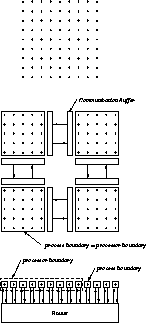
Figure 13.17:
Normal Hypercube Programming Model versus CPC Model for the
Canonical Grid-based Problem. The upper part of the figure shows a
two-dimensional grid upon which the variables of the problem live. The
middle portion shows the usual hypercube model for this type of problem.
There is one process per processor and it contains a subgrid. Some variables
of the subgrid are on a process boundary, some are not. Drawn explicitly are
communication buffers and the channels between them which must be managed by
the programmer. The bottom portion of the figure shows the CPC view of the
same problem. There is one data object (a grid point) for each process so
that all variables are on a process boundary. The router provides a full
interconnect between the processes.
The usual communication calls are not seen at all at the user level.
Variables of other processes (which may or may not be on another
processor) are merely accessed, giving global memory. In our
nCUBE
implementation, this was implemented using the
efficient global communications system called the
crystal_router
(see Chapter 22 of
[
Fox:88a
]).
An actual run-time system was developed for the nCUBE and is described in
[
Felten:88a
]. Much work remains to be done, of course. How to optimize
in order to produce an efficient communications traffic is unexplored; a serious
attempt to produce a fine-grained MIMD machine really involves new types of
hardware, somewhat like Dally's J-machine.
Ed Felten and Steve Otto developed CPC.
Next:
13.7 Hierarchical Memory
Up:
13 Data Parallel C
Previous:
13.5.7 Conclusions
Guy Robinson
Wed Mar 1 10:19:35 EST 1995
13.7 Hierarchical Memory
Next:
14 Asynchronous Applications
Up:
13 Data Parallel C
Previous:
13.6 Coherent Parallel C
In this section, we review some ideas of Fox, dating from 1987, that
unify the decomposition methodologies for hierarchical- and distributed-memory computers [
Fox:87b
]. For a modern workstation, the
hierarchical memory
is formed by the
cache
and main memory. One needs to minimize the cache
misses to ensure that, as far as possible, we reference data in cache
and not in main memory. This is often referred to as the need for
``data locality.''
This term makes clear the
analogy with distributed-memory parallel computers. As shown in this
book, we need data locality in the latter case to avoid communications
between processors. We put the discussion in this chapter because we
anticipate an important application of these ideas to data-parallel
Fortran. The directives in High Performance Fortran essentially
specify data locality and we believe that an HPF compiler
can use the concepts of this
section to optimize cache use on hierarchical-memory machines. Thus,
HPF and similar data-parallel languages will give better performance
than conventional Fortran 77 compilers on
all
high-performance
computers, not just parallel machines.
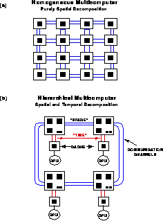
Figure 13.18:
Homogeneous and Hierarchical-Memory Multicomputers. The
black box represents the data that fit into the lowest level of the
memory hierarchy.
Figures
13.18
and
13.19
contrast
distributed-memory multicomputers, shared-memory, and sequential
hierarchical-memory computers. In each case, we denote by a black
square the amount of data which can fit into the lowest level of the
memory hierarchy. In machines such as the nCUBE-1,2 with a simple
node, illustrated in Figure
13.18
(a), this amount is
just what can fit into the node of the distributed-memory computers.
In the other architectures shown in Figures
13.18
and
13.19
, the data corresponding to the black square
represents what can fit into the cache. There is one essential
difference between cache and distributed memory. Both need data
locality, but in the parallel case the basic data is static and
fetches additional information as necessary. This gives the familiar
surface-over-volume communication overheads of
Equation
3.10
. However, in the case of a cache, all the
data must stream through it and not just the data needed to provide
additional information. For distributed-memory machines, we minimize
the need for information flow into and out of a grain as shown in
Figure
3.9
. For hierarchical-memory machines, we need
to maximize the number of times we access the data in cache. These
are related but not identical concepts which we will now compare. We
can use the space-time complex system
language
introduced in Chapter
3
.
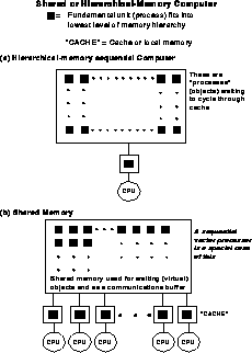
Figure 13.19:
Shared Hierarchical-Memory Computers. ``Cache'' could either
be a time cache or local (software-controlled) memory.
Figure
13.20
introduces a new time constant,  , which is contrasted with
  and
and  introduced in Section
3.5
. The constant
introduced in Section
3.5
. The constant  represents the
time it takes to load a word into cache. As shown in this figure, the
cache overhead is also a ``surface-over-volume'' effect just as it was
in Section
3.5
, but now the surface is measured in the
temporal direction and the volume is that of a domain in space and
time. We find
represents the
time it takes to load a word into cache. As shown in this figure, the
cache overhead is also a ``surface-over-volume'' effect just as it was
in Section
3.5
, but now the surface is measured in the
temporal direction and the volume is that of a domain in space and
time. We find  , time, and memory hierarchy are analogous
to
, time, and memory hierarchy are analogous
to  , space, and distributed memory.
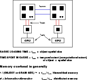
Figure:
The Fundamental Time Constants of a Node. The information
dimension represented by
d
is discussed in Section
3.5
.
Space-time decompositions are illustrated in Figure
13.21
for a simple one-dimensional problem. The decomposition in
Figure
13.21
(a) is fine for distributed-memory machines,
but has poor cache performance. It is blocked in space but not in
time. The optimal decompositions are ``space-time'' blocked and
illustrated in Figure
13.21
(b) and (c).
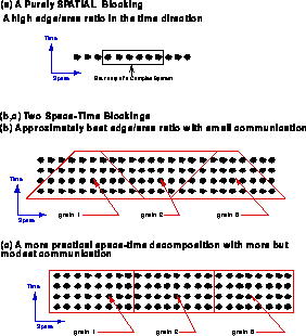
Figure 13.21:
Decompositions for a simple one-dimensional wave equation.
A ``space-time'' blocking is a universal high-performance implementation of
data locality. It will lead to good performance on both distributed-
and hierarchical-memory
machines. This is best
known for the use of the BLAS-3
matrix-matrix primitives in LAPACK
and other matrix
library projects (see Section
8.1
) [
Demmel:91a
]. The
next step is to generate such optimal decompositions from a High
Performance Fortran compiler.
Figure 13.22:
Performance of a Random Surface Fortran Code on Five RISC
Architecture Sequential Computers. The optimizations are described in
the text.
We can illustrate these ideas with the application of
Section
7.2
[
Coddington:93a
]. Table
7.1
records performance of the original code used, but this C version was
improved by an order of magnitude in performance in a carefully
rewritten Fortran code. The relevance of data locality for this
new
code is shown in Figure
13.22
. For each of a set
of five RISC processors, we show four performance numbers gotten by
switching on and off ``system Fortran compiler optimization'' and
``data locality.'' As seen from Section
7.2
, this
application is naturally very irregular and normal data structures do
not express this locality and preserve it. Even if one starts with
neighboring points in the simulated space, ``near'' each other also in
the computer, this is not easily preserved by the dynamic retriangulation.
In the ``data locality'' column, we have arranged storage to preserve
locality as far as possible; neighboring physical points are stored
near each other in memory. A notable feature of
Figure
13.22
is that the Intel i860 shows the largest
improvement from forcing data locality-even after compilation
optimization, this action improves performance by 70%. A similar
result was found in [
Das:92c
] for an unstructured mesh partial
differential equation solver. Other architectures such as the
HP9000-720 with large caches show smaller effects. In
Figure
13.22
, locality was achieved by user manipulation-as
discussed, a next step is to put such intelligence in parallel
compilers.
Next:
14 Asynchronous Applications
Up:
13 Data Parallel C
Previous:
13.6 Coherent Parallel C
Guy Robinson
Wed Mar 1 10:19:35 EST 1995
14 Asynchronous Applications
Next:
Asynchronous Problems and
Up:
Parallel Computing Works
Previous:
13.7 Hierarchical Memory
Guy Robinson
Wed Mar 1 10:19:35 EST 1995
Asynchronous Problems and a Summary of Basic
Problem Classes
Next:
14.2 Melting in Two
Up:
14 Asynchronous Applications
Previous:
14 Asynchronous Applications
Table 14.1:
84 Application Areas Used in a Survey 1988-89 from 400 Papers
The two applications in this chapter fall into the
asynchronous
problem class of Section
3.4
. This class is caricatured in
Figure
14.1
and is the last and hardest to parallelize of
the basic problem architectures
introduced in Section
3.4
. Thus, we will use this opportunity
to summarize some issues across all problem classes. It would be more
logical to do this in Chapter
18
where we discuss the
compound metaproblem
class,
which we now realize is very important. However, the discussion here
is based on a survey [
Fox:88b
], [
Angus:90a
] undertaken from
1988 to 1989, at which time we had not introduced the concept of
compound or hierarchical problem architectures.
Figure 14.1:
The Asynchronous Problem Class
Table
14.1
divides 84 application areas into eight (academic)
disciplines. Examples of the areas are given in the table-essentially each
application section in this book would lead to a separate area for the purposes
of this table.
These areas are listed in [
Angus:90a
], [Fox:88b;92b]
and came a reading in 1988 of about 400 papers which
had developed quite seriously a parallel application or core
nontrivial algorithm. In 1988, it was possible to read essentially
all such papers-the field has grown so much in the following years
that a complete survey would now be a daunting task.
Table
14.2
divides these application areas into the basic
problem architectures used in the book. There are several caveats to
be invoked for this table. As we have seen in Chapters
9
and
12
, the division between synchronous and loosely
synchronous is not sharp and is still a matter of important debate. The
synchronous problems are naturally suitable for SIMD architectures,
while properly loosely synchronous and asynchronous problems require
MIMD hardware. This classification is illustrated by a few of the more
major C P applications in Table
14.3
[
Fox:89t
],
which also compares performance on various SIMD and MIMD machines in
use in 1989.
P applications in Table
14.3
[
Fox:89t
],
which also compares performance on various SIMD and MIMD machines in
use in 1989.
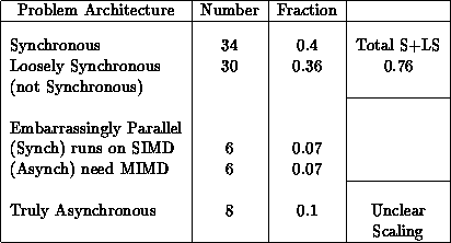
Table 14.2:
Classification of 400 Applications in 84 Areas from 1989.
90% of applications scale to large SIMD/MIMD machines.
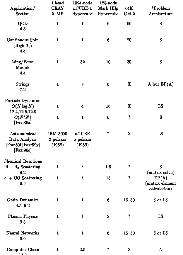
Table 14.3:
Classification of some C P applications from 1989 and
their performances on machines at that time [Fox:89t]. A question mark
indicates the performance is unknown whereas an X indicates we expect or
have measured poor performance.
P applications from 1989 and
their performances on machines at that time [Fox:89t]. A question mark
indicates the performance is unknown whereas an X indicates we expect or
have measured poor performance.
Table
14.2
can be interpreted as follows:
90% of application areas (i.e., all except the asynchronous class)
naturally parallelize to large numbers of processors.
Forty-seven percent of applications will run well on SIMD machines
while 43% need a MIMD architecture (this is a more precise version of
Equation
3.21
).
These numbers are rough for many reasons. The grey line between
synchronous (perhaps generalized to autonomous SIMD in Maspar
language of Section
6.1
) and loosely synchronous means that the
division between SIMD and MIMD fractions is uncertain. Further, how
should one weight each area? QCD of Section
4.3
is one of the
application areas in Table
14.1
, but this uses an
incredible amount of computer time and is a synchronous problem.
Thus, weighting by computer cycles needed or used could also change
the ratios significantly.
These tables can also be used to discuss software issues as described
in Sections
13.1
and
18.2
. The synchronous and
embarrassingly parallel problem classes (54%) are those directly
supported by the initial High Performance Fortran language [
Fox:91e
],
[
Kennedy:93a
]. The loosely synchronous
problems (34%) need run-time and language extensions, which we are
currently working on [
Berryman:91a
], [
Saltz:91b
],
[
Choudhary:92d
], as mentioned in Section
13.1
(Table
13.4
). With these extensions, we expect High
Performance Fortran
to be able to
express nearly all synchronous, loosely synchronous, and embarrassingly
parallel
problems.
The fraction (10%) of asynchronous problems
is in some sense pessimistic. There is one very important
asynchronous area-event driven simulations-where the general
scaling parallelism remains unclear. This is illustrated in
Figure
14.1
and briefly discussed in Section
15.3
.
However, the two cases described in this chapter parallelize
well-albeit with very hard work from the user! Further, some of the
asynchronous areas in Tables
14.1
and
14.2
are of the compound class of
Chapter
18
and these also parallelize well.
The two examples in this chapter need different algorithmic and
software support. In fact, as we will note in Section
15.1
, one
of the hard problems in parallel software is to isolate those issues
that need to be supported over and above those needed for synchronous
and loosely synchronous problems. The software models needed for
irregular statistical mechanics (Section
14.2
), chess
(Section
14.3
), and event-driven simulations
(Section
15.3
) are quite different.
In Section
14.2
, the need for a sequential ordering takes the
normally loosely synchronous time-stepped particle dynamics into an
asynchronous class. Time-stamping the updates provides the necessary
ordering and a ``demand-driven processing queue'' provides scaling
parallelism. Communication must be processed using interrupts and the
loosely synchronous communication style of Section
9.1
will not work.
Another asynchronous application developed by C P was the ray-tracing
algorithm developed by Jeff Goldsmith and John Salmon
[
Fox:87c
],
[Goldsmith:87a;88a]. This application used
two forms of parallelism, with both the pixels (rays) and the basic
model to be rendered distributed. This allows very large models to be
simulated and the covers of our earlier books [
Fox:88a
],
[
Angus:90a
] feature pictures rendered by this program. The
distributed-model database requires software support similar to that
of the application in Section
14.2
. The rays migrate from
node to node as they traverse the model and need to access data not
present in the node currently responsible for ray. This application
was a great technical success, but was not further developed as it
used software (MOOSE of Section
15.2
) which was only
supported on our early machines. The model naturally forms a tree
with the scene represented with increasing spatial resolution as you
go down the different levels of the tree. Goldsmith and Salmon used a
similar strategy to the hierarchical Barnes-Hut approach to particle
dynamics described in Section
12.4
. In particular, the upper
parts of the tree are replicated in all nodes and only the lower parts
distributed. This removes ``sequential bottlenecks''
near the top of the tree just as in the astrophysics case.
Originally, Salmon's thesis intended to study the computer science and
science issues associated with hierarchical data structures.
Multiscale
methods are pervasive to essentially all
physical systems. However, the success of the astrophysical
applications led to this being his final thesis topic. Su, another
student of Fox, has just finished his Ph.D. on the general mathematical
properties of hierarchical systems [
Su:93a
].
P was the ray-tracing
algorithm developed by Jeff Goldsmith and John Salmon
[
Fox:87c
],
[Goldsmith:87a;88a]. This application used
two forms of parallelism, with both the pixels (rays) and the basic
model to be rendered distributed. This allows very large models to be
simulated and the covers of our earlier books [
Fox:88a
],
[
Angus:90a
] feature pictures rendered by this program. The
distributed-model database requires software support similar to that
of the application in Section
14.2
. The rays migrate from
node to node as they traverse the model and need to access data not
present in the node currently responsible for ray. This application
was a great technical success, but was not further developed as it
used software (MOOSE of Section
15.2
) which was only
supported on our early machines. The model naturally forms a tree
with the scene represented with increasing spatial resolution as you
go down the different levels of the tree. Goldsmith and Salmon used a
similar strategy to the hierarchical Barnes-Hut approach to particle
dynamics described in Section
12.4
. In particular, the upper
parts of the tree are replicated in all nodes and only the lower parts
distributed. This removes ``sequential bottlenecks''
near the top of the tree just as in the astrophysics case.
Originally, Salmon's thesis intended to study the computer science and
science issues associated with hierarchical data structures.
Multiscale
methods are pervasive to essentially all
physical systems. However, the success of the astrophysical
applications led to this being his final thesis topic. Su, another
student of Fox, has just finished his Ph.D. on the general mathematical
properties of hierarchical systems [
Su:93a
].
In Section
14.3
, we have a much more irregular and dynamic
problem, computer chess, where statistical methods are used to balance
the processing of the different branches of the dynamically pruned
tree. There is a shared database containing previous evaluation of
positions, but otherwise the processing of the different possible moves
is independent. One does need a clever ordering of the work
(evaluation of the different final positions) to avoid a significant
number of calculations being wasted because they would ``later'' be
pruned away by a parallel calculation on a different processor. Branch
and bound applications [
Felten:88c
], [Fox:87c;88v] [
Fox:87c
]
have similar parallelization characteristics to
computer chess. This was implemented in parallel as a ``best-first''
and not a ``depth-first'' search strategy and was applied to the
travelling salesman problem (Section
11.4
) to find exact solutions
to test the physical optimization
algorithms. It was also applied to
the 0/1 knapsack problem, but for this and TSP, difficulties arose due
to insufficient memory for holding the queues of unexplored subtrees.
The depth-first strategy, used in our parallel computer chess program
and sequential branch and bound, avoids the need for large memory. On
sequential machines, virtual memory can be used for the subtree queues,
but this was not implemented on the nCUBE-1 and indeed is absent on
most current multicomputers.
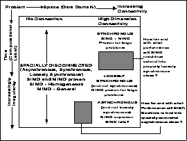
Figure 14.2:
Issues Affecting Relation of Machine, Problem, and Software
Architecture
The applications in this chapter are easier than a full event-driven
simulation because enough is known about the problem to find a
reasonable parallel algorithm. The difficulty then, is to make it
efficient. Figure
14.2
is a schematic of problem
architectures labelled by spatial and temporal properties. In
general, the temporal characteristics-the problem
architectures
(synchronous, loosely
synchronous and asynchronous)-determine the nature of the
parallelism. One special case is the
spatially disconnected
problem class for which the temporal characteristic is essentially
irrelevant. For the general
spatially connected
class, the
nature of this connection will affect performance and ease, but not the
nature of their parallelism. These issues are summarized in
Table
14.4
. For instance, spatially irregular problems,
such as those in Chapter
12
, are particularly hard to implement
although they have natural parallelism. The applications in this
chapter can be viewed as having little spatial connectivity and their
parallelism comes because, although asynchronous, they are ``near'' the
spatially disconnected class of Figure
14.2
.
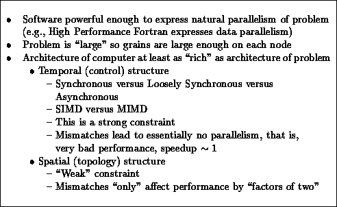
Table 14.4:
Criterion for success in parallelizing a particular problem
on a particular machine.
Next:
14.2 Melting in Two
Up:
14 Asynchronous Applications
Previous:
14 Asynchronous Applications
Guy Robinson
Wed Mar 1 10:19:35 EST 1995
14.2 Melting in Two Dimensions
Next:
14.2.1 Problem Description
Up:
14 Asynchronous Applications
Previous:
Asynchronous Problems and
Guy Robinson
Wed Mar 1 10:19:35 EST 1995
14.2.1 Problem Description
Next:
14.2.2 Solution Method
Up:
14.2 Melting in Two
Previous:
14.2 Melting in Two
Although we live in a three-dimensional world, many important processes
involve interactions on surfaces, which are effectively
two-dimensional. While experimental studies of two-dimensional systems
have been successful in probing some aspects of such systems, computer
simulation is another powerful tool that can be used to measure their
properties. We have used a computer simulation to study the
melting
transition of a two-dimensional system of
interacting particles
[Johnson:86a;86b]. One purpose of the study is to investigate whether
melting in two dimensions occurs through a qualitatively different
process than it does it three dimensions. In three dimensions, the
melting transition is a first-order transition which displays a
characteristic latent heat. Halperin and Nelson [
Halperin:78a
],
[
Nelson:79a
] and Young [
Young:79a
] have raised the
possibility that melting in two dimensions could occur through a
qualitatively different process. They have suggested that melting
could consist of a pair of higher-order phase transitions,
which lack a latent heat, that are driven by topological
defects in the two-dimensional crystal lattice.
We studied a two-dimensional system of particles interacting through a
truncated Lennard-Jones potential.
The
Lennard-Jones potential is
where  is the energy parameter,
  is the length parameter,
and
r
is the distance between two particles. The potential is attractive
at distances larger than
is the length parameter,
and
r
is the distance between two particles. The potential is attractive
at distances larger than  and repulsive smaller distances. The
potential energy of the whole system is the sum of the potential energies of
each pair of interacting particles. In order to ease the computational
requirements of the simulation, we have truncated the potential at a particle
separation of
and repulsive smaller distances. The
potential energy of the whole system is the sum of the potential energies of
each pair of interacting particles. In order to ease the computational
requirements of the simulation, we have truncated the potential at a particle
separation of  .
.
Mark A. Johnson wrote the Monte Carlo
simulation of
melting in two dimensions for his Ph.D. research at Caltech.
Guy Robinson
Wed Mar 1 10:19:35 EST 1995
14.2.2 Solution Method
Next:
14.2.3 Concurrent Update Procedure
Up:
14.2 Melting in Two
Previous:
14.2.1 Problem Description
We chose to use a Monte Carlo
method to simulate the
interaction of the
particles. The method consists of generating a sequence of configurations in
such a way that the probability of being in configuration
r
, denoted as
 , is
, is

where  is the potential energy of configuration
r
and
is the potential energy of configuration
r
and  .
A configuration refers collectively to the positions of all the particles in
the simulation. The update procedure that we describe in the next section
generates such a sequence of configurations by repeatedly updating the
position of each of the particles in the system. Averaging the values of
such quantities as potential energy and pressure over the configurations
gives their expected values in such a system.
.
A configuration refers collectively to the positions of all the particles in
the simulation. The update procedure that we describe in the next section
generates such a sequence of configurations by repeatedly updating the
position of each of the particles in the system. Averaging the values of
such quantities as potential energy and pressure over the configurations
gives their expected values in such a system.
The process of moving from one configuration to another is known as a Monte
Carlo update. The update procedure we used involves three steps that allow
the position of one particle to change
[
Metropolis:53a
].
The first step is to choose a
new position for the particle with uniform probability in a region
about its current position. Next, the update procedure calculates the
difference in potential energy between the current configuration and
the new one. Finally, the new position for the particle is either
accepted or rejected based on the difference in potential energy and
rules that generate configurations with the required probability
distribution.
The two-dimensional system being studied has several characteristics that
must be considered in designing an efficient algorithm for implementing the
Monte Carlo simulation. One of the most important characteristics is that
the interaction potential has a short range. The Lennard-Jones potential
approaches zero quickly enough that the effect of distant particles can be
safely ignored. We made the short-range nature of the potential precise by
truncating it at a distance of  . We must use the short-range nature
of the potential to organize the particle positions so that the update
procedure can quickly locate the particles whose potential energy changes
during an update.
. We must use the short-range nature
of the potential to organize the particle positions so that the update
procedure can quickly locate the particles whose potential energy changes
during an update.
Another feature of the system that complicates the simulation is that the
particles are not confined to a grid that would structure the data. Such
irregular data make simultaneously updating multiple particles more
difficult. One result of the irregular data is that the computational loads
of the processors are unbalanced in a distributed-memory, MIMD processor. In
order to minimize the effect of the load imbalance, the nodes of the
concurrent processor must run asynchronously.
We developed an interrupt-driven
communication system [
Johnson:85a
] that allows the nodes to
implement an asynchronous update procedure. This ``
rdsort
''
system is described in Section
5.2.5
and has similarities to
the current active message ideas [
Eiken:92a
]. The
interrupt-driven communication system allows a node to send requests
for contributions to the change in potential energy that moving its
particle would cause. Nodes receiving such requests compute the
contribution of their particles and send a response reporting their
result. This operating system was sophisticated but only used for this
application. However, as described in Chapter
5
, these ideas
formed the basis of both MOOS II and the evolution of CrOS III into
Express. Interestingly, Mark Johnson designed the loosely synchronous
CrOS III message-passing system as part of his service for C P even
though his particular application was one of the few that could not
benefit from it.
P even
though his particular application was one of the few that could not
benefit from it.
Next:
14.2.3 Concurrent Update Procedure
Up:
14.2 Melting in Two
Previous:
14.2.1 Problem Description
Guy Robinson
Wed Mar 1 10:19:35 EST 1995
14.2.3 Concurrent Update Procedure
Next:
14.2.4 Performance Analysis
Up:
14.2 Melting in Two
Previous:
14.2.2 Solution Method
Performing Monte Carlo updates in parallel requires careful attention to
ensuring that simultaneous updates do not interfere with each other. Because
the basic equations governing the Monte Carlo method remain unchanged,
performing the updates in parallel requires that a consistent sequential
ordering of the updates exists. No
particular
ordering is
required; only the existence of such an ordering is critical.
Particles that are farther apart than the range of the interaction
potential cannot influence each other, so any arbitrary ordering of
their updates is always consistent. However, if some of the particles
being updated together are within the range of the potential, they
cannot be updated as if they were independent because the result of one
update affects the others. Fortunately, the symmetry of the potential
guarantees that all of the affected particles are aware that their
updates are interdependent.
Note that the Monte Carlo approach to melting or, more generally, any
particle simulation is often much harder to parallelize than the competitive
time-stepped evolution approach. The latter would be loosely
synchronous with natural parallelism. The need for a consistent
sequential ordering in the Monte Carlo algorithm leads to the
asynchronous temporal structure.
It is
interesting that on a sequential machine, both time-stepped and Monte
Carlo methods would be equally easy to implement. However, even here
the sequential ordering for the Monte Carlo would make it hard to
vectorize the algorithm on a conventional supercomputer. In discussing
regular Monte Carlo problems such as QCD in Section
4.3
, the
sequential ordering constraint is there but trivial to implement, as
the regular spatial structure allows one to predetermine a consistent
update procedure. In particular, the normal red-black update structure
achieves this. In the melting problem, one has a dynamically varying
irregularity that allows no simple way of predetermining a consistent
Monte Carlo update schedule.
Each node involved in the conflicting updates must act to resolve the
situation by making one of only two possible decisions. For each request for
contributions to the difference in potential energy of an update, a node can
either send a response immediately or delay the response until its own update
finishes. If the node sends the response immediately, it must use the old
position of the particle that it is updating. If the node instead delays the
response while waiting for its own update to finish, it will use the new
position of the particle when its update finishes. If all of the nodes
involved in the conflicting updates make consistent decisions, a sequential
ordering of the updates will exist, ensuring the correctness of the Monte
Carlo procedure. However, if two nodes both decide to send responses to each
other based on the current positions of the particles they are updating, no
such ordering will exist. If two nodes both decide to delay sending
responses to each other, neither will be able to complete their update,
causing the simulation to deadlock.
Several features of the concurrent update procedure make resolving such
interdependent updates difficult. Each node must make its decision regarding
the resolution of the conflicting updates in isolation from the other nodes
because all of the nodes are running asynchronously to minimize load
imbalance. However, the nodes cannot run completely asynchronously because
assigning a consistent sequential ordering to the updates requires that the
update procedure impose a synchronizing
condition on
the updates. Still, the
condition should be as weak as possible so that the decrease in processing
efficiency is minimized.
One solution to the problem of correctly ordering interdependent updates
requires that a clock exist in each of the nodes. The update procedure
records the time at which it begins updating a particle and includes that
time with each of its requests for contributions to the difference in
potential energy. When a node determines that its update conflicts with that
of another node, it uses the times of the conflicting updates to resolve the
dependence. The node sends a response immediately if the request involves an
update that precedes its own. The node delays sending a response if its own
update precedes the one that generated the request. Should the times be
exactly equal, the unique number associated with each node provides a means
of consistently ordering the updates. When each of the processors involved
in the conflicting updates use such a method to resolve the situation, a
consistent sequential ordering must result. Using the time of each of the
conflicting updates to determine their ordering allows the earliest updates
to finish first, which achieves good load balance
in the concurrent algorithm.
Although delaying a response to a conflicting update is a synchronizing
condition, it is sufficiently weak that it does not seriously degrade the
performance of the concurrent algorithm. A node can respond to other nodes'
requests while waiting for responses to requests that it has generated. The node
that delays sending a response can perform most of the computation to
generate the response while it is waiting for responses to its own requests,
because the position of only one particle is in question. In fact, the
current implementation simply generates the two possible responses so that it
can send the correct response immediately after its own update completes.
An interesting feature of the concurrent update algorithm is that it produces
results that are inherently irreproducible. If two simulations start with
exactly the same initial data, including random number
seeds, the simulations will eventually differ. The source of
the irreproducible behavior is that all components of the concurrent
processor are not driven by the same clock. For instance, the
communication channels that connect the nodes contain an asynchronous
loop that allows the arrival times of messages to differ by arbitrarily
small amounts. Such differences can affect the order in which requests
are received, which in turn determines the order in which a node
generates responses. Once such differences change the outcome of a
single update, the two simulations begin to evolve independently. Both
simulations continue to generate configurations with the correct
probability distribution, so the statistical properties of the
simulations do not change. However, the irreproducible behavior of the
concurrent update algorithm can make debugging
somewhat more difficult.
Next:
14.2.4 Performance Analysis
Up:
14.2 Melting in Two
Previous:
14.2.2 Solution Method
Guy Robinson
Wed Mar 1 10:19:35 EST 1995
14.2.4 Performance Analysis
Next:
14.3 Computer Chess
Up:
14.2 Melting in Two
Previous:
14.2.3 Concurrent Update Procedure
Because a complete performance analysis of the Monte Carlo simulation is
rather lengthy, we provide only a summary of the analysis here. Calculating
the efficiency of the concurrent update algorithm is relatively simple
because it requires only measurements of the time an update takes on one node
and on multiple nodes. A more difficult parameter to calculate is
the load balance of the update procedure. In order to calculate the load
balance, we measured the time required to send each type of message that the
update uses. The total communication overhead is the sum of the overheads
for each type of message, which is the product of the time to send that type
of message and the number of such messages. We calculated the number of each
type of message by assuming a uniform distribution of particles. Because the
update algorithm contains no significant serial components, we attributed to
load imbalance the parallel overhead remaining after accounting for the
communication overhead. The load balance is a factor that can range from
 , where
N
is the number of nodes, to 1, which occurs when the loads
are balanced perfectly. We give the update time in seconds, the efficiency,
and the load balance for several simulations on the 64-node Caltech hypercube
in Table
14.5
([
Johnson:86a
] p. 73).
, where
N
is the number of nodes, to 1, which occurs when the loads
are balanced perfectly. We give the update time in seconds, the efficiency,
and the load balance for several simulations on the 64-node Caltech hypercube
in Table
14.5
([
Johnson:86a
] p. 73).
Table 14.5:
Simulations on the 64-node Caltech Hypercube
Guy Robinson
Wed Mar 1 10:19:35 EST 1995
14.3 Computer Chess
Next:
14.3.1 Sequential Computer Chess
Up:
14 Asynchronous Applications
Previous:
14.2.4 Performance Analysis
As this book shows, distributed-memory, multiple-instruction stream
(MIMD) computers are successful in performing a large class of
scientific computations. As discussed in Section
14.1
and the
earlier chapters, these synchronous and loosely synchronous problems
tend to have regular, homogeneous data sets and the algorithms are
usually ``crystalline'' in nature. Recognizing this, C P explored
a set of algorithms which had irregular structure (as in
Chapter
12
) and asynchronous execution. At the start of this
study, we were very unclear as to what parallel performance to expect.
In fact, we achieved good speedup even in these hard problems.
P explored
a set of algorithms which had irregular structure (as in
Chapter
12
) and asynchronous execution. At the start of this
study, we were very unclear as to what parallel performance to expect.
In fact, we achieved good speedup even in these hard problems.
Thus, as an attempt to explore a part of this interesting, poorly
understood region in algorithm space, we implemented chess
on an nCUBE-1
hypercube. Besides being a
fascinating field of study in its own right, computer chess is an
interesting challenge for parallel computers because:
-
It is not clear how much parallelism is actually available-the
important method of alpha-beta pruning conflicts with parallelism.
-
Some aspects of the algorithm require a globally shared data set.
-
The parallel algorithm has dynamic load imbalance of an extreme nature.
One might also ask the question, ``Why study computer chess at all?'' We
think the answer lies in the unusual position of computer chess within the
artificial intelligence world. Like most AI problems, chess requires a
program which will display seemingly intelligent behavior in a limited,
artificial world. Unlike most AI problems, the programmers do not get to make
up the rules of this world. In addition, there is a very rigorous procedure
to test the intelligence of a chess program-playing games against humans.
Computer chess is one area where the usually disparate worlds of AI and
high-performance computing meet.
Before going on, let us state that our approach to parallelism (and hence
speed) in computer chess is not the only one. Belle, Cray
Blitz, Hitech, and the current champion, Deep Thought have shown in
spectacular fashion that fine-grained parallelism (pipelining,
specialized hardware) leads to impressive speeds (see [
Hsu:90a
],
[
Frey:83a
], [
Marsland:87a
], [
Ebeling:85a
],
[
Welsh:85a
]). Our coarse-grained approach to parallelism should
be viewed as a complementary, not a conflicting, method. Clearly the
two can be combined.
Next:
14.3.1 Sequential Computer Chess
Up:
14 Asynchronous Applications
Previous:
14.2.4 Performance Analysis
Guy Robinson
Wed Mar 1 10:19:35 EST 1995
14.3.1 Sequential Computer Chess
Next:
The Evaluation Function
Up:
14.3 Computer Chess
Previous:
14.3 Computer Chess
In this section we will describe some basic aspects of what constitutes a
good chess program on a sequential computer. Having done this, we will be
able to intelligently discuss the parallel algorithm.
At present, all competitive chess programs work by searching a tree of
possible moves and countermoves. A program starts with the current board
position and generates all legal moves, all legal responses to these moves,
and so on until a fixed depth is reached. At each leaf node, an evaluation
function is applied which assigns a numerical score to that board position.
These scores are then ``backed up'' by a process called minimaxing, which is
simply the assumption that each side will choose the line of play most
favorable to it at all times. If positive scores favor white, then white
picks the move of maximum score and black picks the move of minimum score.
These concepts are illustrated in Figure
14.3
.
Figure 14.3:
Game Playing by Tree Searching. The top half of the figure
illustrates the general idea: Develop a full-width tree to some
depth, then score the leaves with the evaluation function,
f
. The
second half shows minimaxing-the reasonable supposition that white
(black) chooses lines of play which maximize (minimize) the score.
The evaluation function employed is a combination of simple material balance
and several terms which represent positional factors. The positional terms
are small in magnitude but are important since material balance rarely
changes in tournament chess games.
The problem with this brute-force approach is that the size of the tree
explodes exponentially. The ``branching factor'' or number of legal moves
in a typical position is about 35. In order to play master-level chess
a search of depth eight appears necessary, which would involve a tree of
 or about
  leaf nodes.
Fortunately, there is a better way. Alpha-beta
pruning
is a technique which always gives the
same answer as brute-force searching without looking at so many nodes
of the tree. Intuitively, alpha-beta pruning works by ignoring
subtrees which it knows cannot be reached by best play (on the part of
both sides). This reduces the effective branching factor from 35 to
about 6, which makes strong play possible.
The idea of alpha-beta pruning is illustrated in Figure
14.4
.
Assume that all child nodes are searched in the order of left to right in the
figure. On the left side of the tree (the first subtree searched), we have
minimaxed and found a score of
+4
at depth one. Now, start to analyze the
next subtree. The children report back scores of
+5
,
-1
,  . The
pruning happens after the score of
-1
is returned: since we are taking
the minimum of the scores
+5
,
-1
,
. The
pruning happens after the score of
-1
is returned: since we are taking
the minimum of the scores
+5
,
-1
,  , we immediately have a bound on
the scores of this subtree-we know the score will be no larger than
-1
.
Since we are taking the maximum at the next level up (the root of the tree)
and we already have a line of play better than
-1
(namely, the
+4
subtree), we need not explore this second subtree any further. Pruning
occurs, as denoted by the dashed branch of the second subtree. The process
continues through the rest of the subtrees.
, we immediately have a bound on
the scores of this subtree-we know the score will be no larger than
-1
.
Since we are taking the maximum at the next level up (the root of the tree)
and we already have a line of play better than
-1
(namely, the
+4
subtree), we need not explore this second subtree any further. Pruning
occurs, as denoted by the dashed branch of the second subtree. The process
continues through the rest of the subtrees.
Figure:
Alpha-Beta Pruning for the Same Tree as
Figure
14.3
. The tree is generated in left-to-right
order. As soon as the score
-1
is computed, we immediately have a
bound on the level above ( ) which is below the score of the
+4
subtree. A cutoff occurs, meaning no more descents of the
) which is below the score of the
+4
subtree. A cutoff occurs, meaning no more descents of the  node
need to be searched.
node
need to be searched.
The amount of work saved in this small tree was insignificant but alpha-beta
becomes very important for large trees. From the nature of the pruning
method, one sees that the tree is not evolved evenly downward. Instead, the
algorithm pursues one branch all the way to the bottom, gets a ``score to
beat'' (the alpha-beta bounds), and then sweeps across the tree sideways.
How well the pruning works depends crucially on move ordering. If the best
line of play is searched first, then all other branches will prune
rapidly.
Actually, what we have discussed so far is not full alpha-beta pruning, but
merely ``pruning without deep cutoffs.'' Full alpha-beta pruning shows up
only in trees of depth four or greater. A thorough discussion of alpha-beta
with some interesting historical comments can be found in Knuth and Moore
[
Knuth:75a
].
Next:
The Evaluation Function
Up:
14.3 Computer Chess
Previous:
14.3 Computer Chess
Guy Robinson
Wed Mar 1 10:19:35 EST 1995
The Evaluation Function
Next:
Quiescence Searching
Up:
14.3.1 Sequential Computer Chess
Previous:
14.3.1 Sequential Computer Chess
The evaluation function of our program is similar in style to that of the
Cray
Blitz program [
Welsh:85a
]. The most important
term is material, which is a simple count of the number of pieces on
each side, modified by a factor which encourages the side ahead in
material to trade pieces but not pawns. The material evaluator also
recognizes known draws such as king and two knights versus king.
There are several types of positional terms, including pawn structure, king
safety, center control, king attack, and specialized bonuses for things like
putting rooks on the seventh rank.
The pawn structure evaluator knows about doubled, isolated, backward, and
passed pawns. It also has some notion of pawn chains and phalanxes. Pawn
structure computation is very expensive, so a hash table is used to store the
scores of recently evaluated pawn structures. Since pawn structure changes
slowly, this hash table almost always saves us the work of pawn structure
evaluation.
King safety is evaluated by considering the positions of all pawns on the
file the king is occupying and both neighboring files. A penalty is assessed
if any of the king's covering pawns are missing or if there are holes
(squares which can never be attacked by a friendly pawn) in front of the
king. Additional penalties are imposed if the opponent has open or
half-open files near the king. The whole king safety score is multiplied
by the amount of material on the board, so the program will want to trade
pieces when its king is exposed, and avoid trades when the opponent's king
is exposed. As in pawn structure, king safety uses a hash table to avoid
recomputing the same information.
The center control term rewards the program for posting its pieces safely
in the center of the board. This term is crude since it does not consider
pieces attacking the center from a distance, but it can be computed very
quickly and it encourages the kind of straightforward play we want.
King attack gives a bonus for placing pieces near the opposing king. Like
center control, this term is crude but tends to lead to positions in which
attacking opportunities exist.
The evaluation function is rounded out by special bonuses to encourage
particular types of moves. These include a bonus for castling, a penalty
for giving up castling rights, rewards for placing rooks on open and
half-open files or on the seventh rank, and a penalty for a king on the back
rank with no air.
Next:
Quiescence Searching
Up:
14.3.1 Sequential Computer Chess
Previous:
14.3.1 Sequential Computer Chess
Guy Robinson
Wed Mar 1 10:19:35 EST 1995
Quiescence Searching
Next:
Iterative Deepening
Up:
14.3.1 Sequential Computer Chess
Previous:
The Evaluation Function
Of course it only makes sense to apply a static evaluation function to a
position which is quiescent, or tactically quiet. As a result, the tree is
extended beyond leaf nodes until a quiescent position is reached, where
the static evaluator is actually applied.
We can think of the quiescence search as a dynamic evaluation function, which
takes into account tactical possibilities. At each leaf node, the side to
move has the choice of accepting the current static evaluation or of trying
to improve its position by tactics. Tactical moves which can be tried
include pawn promotions, most capture moves, some checks, and some pawn
promotion threats. At each newly generated position the dynamic evaluator is
applied again. At the nominal leaf nodes, therefore, a narrow (small
branching factor) tactical search is done, with the static evaluator applied
at all terminal points of this search (which end up being the true leaves).
Guy Robinson
Wed Mar 1 10:19:35 EST 1995
Iterative Deepening
Next:
The Hash Table
Up:
14.3.1 Sequential Computer Chess
Previous:
Quiescence Searching
Tournament chess is played under a strict time control, and a program must
make decisions about how much time to use for each move. Most chess programs
do not set out to search to a fixed depth, but use a technique called
iterative deepening.
This means a program
does a depth two search, then a depth three search, then a depth four
search, and so on until the allotted time has run out. When the time
is up, the program returns its current best guess at the move to make.
Iterative deepening has the additional advantage that it facilitates move
ordering. The program knows which move was best at the previous level of
iterative deepening, and it searches this principal variation first at
each new level. The extra time spent searching early levels is more than
repaid by the gain due to accurate move ordering.
Guy Robinson
Wed Mar 1 10:19:35 EST 1995
The Hash Table
Next:
The Opening
Up:
14.3.1 Sequential Computer Chess
Previous:
Iterative Deepening
During the tree search, the same board position may occur several times.
There are two reasons for this. The first is transposition, or the fact
that the same board position can be reached by different sequences of moves.
The second reason is iterative deepening-the same position will be reached
in the depth two search, the depth three search, and so on. The hash table is a way
of storing information about positions which have already been searched; if
the same position is reached again, the search can be sped up or eliminated
entirely by using this information.
The hash table plays a central role in a good chess program and so we
will describe it in some detail. First of all, the hash table is a
form of content-addressable memory-with each chess board (a node in
the chess tree) we wish to associate some slot in the table. Therefore,
a hashing function
h
is required, which maps chess boards to slots in
the table. The function
h
is designed so as to scatter similar
boards across the table. This is done because in any single search the
boards appearing in the tree differ by just a few moves and we wish to
avoid collisions (different boards mapping to the same slot) as much as
possible. Our hash function is taken from [
Zobrist:70a
]. Each
slot in the table contains
-
the known bounds on the score of this position;
-
the depth to which these bounds are valid;
-
a suggested move to try;
-
a staleness flag; and
-
a 64-bit collision check
Instead of just blindly generating all legal moves at a position and then
going down these lines of play, the hash table is first queried about the
position. Occasionally, the hash table bounds are so well-determined as to
cause an immediate alpha-beta cutoff. More often, the hash table has a
suggested move to try and this is searched first. The 64-bit collision check
is employed to ensure that the slot has information about the same position
that the program is currently considering (remember, more than one chess
board can map to the same slot in the table).
Whenever the program completes the search of a subtree of substantial size
(i.e., one of depth greater than some minimum), the knowledge gained is
written into the hash table. The writing is not completely naive, however.
The table contains only a finite number of slots, so collisions occur;
writeback acts to keep the most valuable information. The depth field
of the slot helps in making the decision as to what is most valuable. The
information coming from the subtree of greater depth (and hence, greater
value) is kept.
The staleness flag allows us to keep information from one search to the next.
When time runs out and a search is considered finished, the hash table is not
simply cleared. Instead, the staleness flag is set in all slots. If, during
the next search, a read is done on a stale slot the staleness flag is
cleared, the idea being that this position again seems to be useful. On
writeback, if the staleness flag is set, the slot is simply overwritten,
without checking the depths. This prevents the hash table from becoming
clogged with old information.
Proper use of an intelligent hash table such as the one described above gives
one, in effect, a ``principal variation'' throughout the chess tree. As
discussed in [
Ebeling:85a
], a hash table can effectively give
near-perfect move ordering and hence, very efficient pruning.
Next:
The Opening
Up:
14.3.1 Sequential Computer Chess
Previous:
Iterative Deepening
Guy Robinson
Wed Mar 1 10:19:35 EST 1995
The Opening
Next:
The Endgame
Up:
14.3.1 Sequential Computer Chess
Previous:
The Hash Table
The opening is played by making use of an ``opening book'' of known positions.
Our program knows the theoretically ``best'' move in about 18,000 common
opening positions. This information is stored as a hash table on disk and can
be looked up quickly. This hash table resolves collisions through the method
of chaining [
Knuth:73a
].
Guy Robinson
Wed Mar 1 10:19:35 EST 1995
The Endgame
Next:
14.3.2 Parallel Computer Chess:
Up:
14.3.1 Sequential Computer Chess
Previous:
The Opening
Endgames are handled by using special evaluation functions which contain
knowledge about endgame principles. For instance, an evaluator for king and
pawn endgames may be able to directly recognize a passed pawn which can race
to the last rank without being caught by the opposing king. Except for the
change in evaluation functions, the endgame is played in the same fashion as
the middlegame.
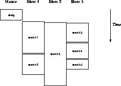
Figure 14.5:
Slaves Searching Subtrees in a Self-scheduled Manner. Suppose
one of the searches-in this case search two-takes a long time. The
advantage of self-scheduling is that, while this search is
proceeding in slave two, the other slaves will have done all the
remaining work. This very general technique works as long as the
dynamic range of the computation times is not too large.
Guy Robinson
Wed Mar 1 10:19:35 EST 1995
14.3.2 Parallel Computer Chess: The Hardware
Next:
14.3.3 Parallel Alpha-Beta Pruning
Up:
14.3 Computer Chess
Previous:
The Endgame
Our program is implemented on an nCUBE/10 system. This is an MIMD (multiple
instruction stream, multiple data stream) multicomputer, with each node
consisting of a custom VLSI
processor running at 7 MHz,
512 Kbytes of memory, and on-chip communication channels. There is no
shared
memory-processors communicate by
message-passing. The nodes are connected as a hypercube but the VERTEX
message-passing software [
nCUBE:87a
] gives the illusion of full
connectivity. The nCUBE system at Caltech has 512 processors, but
systems exist with as many as 1024 processors. The program is written
in C, with a small amount of assembly code.
Guy Robinson
Wed Mar 1 10:19:35 EST 1995
14.3.3 Parallel Alpha-Beta Pruning
Next:
Analysis of Alpha-Beta
Up:
14.3 Computer Chess
Previous:
14.3.2 Parallel Computer Chess:
Some good chess programs do run in parallel (see [
Finkel:82a
],
[
Marsland:84a
], [
Newborn:85a
], [Schaeffer:84a;86a]),
but before our work
nobody had tried more than about 15 processors. We were interested in
using hundreds or thousands of processors. This forced us to squarely
face all the issues of parallel chess-algorithms which work for a few
processors do not necessarily scale up to hundreds of processors. An
example of this is the occurrence of sequential bottlenecks
in the control structure of the program. We have been very
careful to keep control of the program decentralized so as to avoid
these bottlenecks.
The parallelism comes from searching different parts of the chess tree
at the same time. Processors are organized in a hierarchy with one
master processor controlling several teams, each submaster controlling
several subteams, and so on. The basic parallel operation consists of
one master coming to a node in the chess tree, and assigning subtrees
to his slaves in a self-scheduled way. Figure
14.5
shows a
timeline of how this might happen with three subteams. Self-scheduling
by the slaves helps to load-balance the computation, as can be seen in
the figure.
So far, we have defined what happens when a master processor reaches a node
of the chess tree. Clearly, this process can be repeated recursively. That
is, each subteam can split into sub-subteams at some lower level in the tree.
This recursive splitting process, illustrated in Figure
14.6
,
allows large numbers of processors to come into play.
In conflict with this is the inherent sequential model of the standard
alpha-beta algorithm. Pruning depends on fully searching one subtree in
order to establish bounds (on the score) for the search of the next subtree.
If one adheres to the standard algorithm in an overly strict manner, there
may be little opportunity for parallelism. On the other hand, if one is too
naive in the design of a parallel algorithm, the situation is easily reached
where the parallel program searches an impressive number of board positions
per second, but still does not search much more deeply than a single
processor running the alpha-beta algorithm. The point is that one should not
simply split or ``go parallel'' at every opportunity-as we will see below,
it is sometimes better to leave processors idle for short periods of time and
then do work at more effective points in the chess tree.
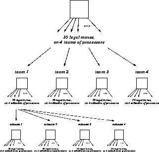
Figure:
The Splitting Process of Figure
14.5
is Now
Repeated, in a Recursive Fashion, Down the Chess Tree to Allow Large
Numbers of Processors to Come into Play. The topmost master has four
slaves, which are each in turn an entire team of processors, and so on.
This figure is only approximate, however. As explained in the text, the
splitting into parallel threads of computation is not done at every
opportunity but is tightly controlled by the global hash table.
Next:
Analysis of Alpha-Beta
Up:
14.3 Computer Chess
Previous:
14.3.2 Parallel Computer Chess:
Guy Robinson
Wed Mar 1 10:19:35 EST 1995
Analysis of Alpha-Beta Pruning
Next:
Global Hash Table
Up:
14.3.3 Parallel Alpha-Beta Pruning
Previous:
14.3.3 Parallel Alpha-Beta Pruning
The standard source on mathematical analysis of the alpha-beta algorithm is
the paper by Knuth and Moore [
Knuth:75a
]. This paper gives a complete
analysis for perfectly ordered trees, and derives some results about randomly
ordered trees. We will concern ourselves here with perfectly ordered trees,
since real chess programs achieve almost-perfect ordering.
Figure:
Pruning of a Perfectly Ordered Tree. The tree of
Figures
14.3
and
14.4
has
been extended another ply, and also the move ordering has been
rearranged so that the best move is always searched first. By
classifying the nodes into types as described in the text, the following
pattern emerges: All children of type one and three nodes are
searched, while only the first child of a type two node is searched.
In this context, perfect move-ordering means that in any position, we always
consider the best move first. Ordering of the rest of the moves does not
matter. Knuth and Moore show that in a perfectly ordered tree, the nodes
can be divided into three types, as illustrated by Figure
14.7
.
As in previous figures, nodes are assumed to be generated and searched in
left-to-right order. The typing of the nodes is as follows. Type one nodes
are on the ``principal variation.'' The first child of a type one node is
type one and the rest of the children are type two. Children of type two
nodes are type three, and children of type three nodes are type two.
How much parallelism is available at each node? The pruning of the perfectly
ordered tree of Figure
14.7
offers a clue. By thinking through
the alpha-beta procedure, one notices the following pattern:
-
All children of type one nodes are searched,
-
Only the first child of a type two node is searched-the rest are
pruned; and
-
All children of type three nodes must be searched.
This oscillating pattern between the node types is, of course, the reason for
distinguishing them as different types in the first place.
The implications of this for a parallel search are important. To efficiently
search a perfectly ordered tree in parallel, one should perform the following
algorithm.
-
At type one nodes, the first child must be searched sequentially (in
order to initialize the alpha-beta bounds), then the rest can be searched in
parallel.
-
At type two nodes, there is no parallelism since only one child will be
searched (time spent searching other children will be wasted).
-
Type three nodes, on the other hand, are fully parallel and all the
children can be searched independently and simultaneously.
The key for parallel search of perfectly ordered chess trees, then, is to
stay sequential at type two nodes, and go parallel at type three nodes. In
the non-perfectly ordered case, the clean distinction between node types
breaks down, but is still approximately correct. In our program, the
hash table plays a role in deciding upon the node type. The following
strategy is used by a master processor when reaching a node of the chess tree:
Make an inquiry to the hash table regarding this position. If the
hash table suggests a move, search it first, sequentially. In this context,
``sequentially'' means that the master takes her slaves with her down this
line of play. This is to allow possible parallelism lower down in the tree.
If no move is suggested or the suggested move fails to cause an alpha-beta
cutoff, search the remaining moves in parallel. That is, farm the work out
to the slaves in a self-scheduled manner.
This parallel algorithm is intuitively reasonable and also reduces to the
correct strategy in the perfectly ordered case. In actual searches, we have
explicitly (on the nCUBE graphics monitor) observed the sharp classification
of nodes into type two and type three at alternate levels of the chess tree.
Next:
Global Hash Table
Up:
14.3.3 Parallel Alpha-Beta Pruning
Previous:
14.3.3 Parallel Alpha-Beta Pruning
Guy Robinson
Wed Mar 1 10:19:35 EST 1995
Global Hash Table
Next:
14.3.4 Load Balancing
Up:
14.3.3 Parallel Alpha-Beta Pruning
Previous:
Analysis of Alpha-Beta
The central role of the hash table in providing refutations and telling the
program when to go parallel makes it clear that the hash table must be shared
among all processors. Local hash tables would not work since the complex,
dynamically changing organization of processors makes it very unlikely that a
processor will search the same region of the tree in two successive levels of
iterative deepening. A shared table is expensive on a distributed-memory
machine, but in this case it is worth it.
Each processor contributes an equal amount of memory to the shared hash table.
The global hash function maps each chess position to a global slot number
consisting of a processor ID and a local slot number. Remote memory is
accessed by sending a message to the processor in which the desired memory
resides. To insure prompt service to remote memory requests, these messages
must cause an interrupt on arrival. The VERTEX system does not support this
feature, so we implemented a system called
generalized signals
[
Felten:88b
], which allows interrupt-time servicing of some messages
without disturbing the running program.
When a processor wants to read a remote slot in the hash table, it sends a
message containing the local slot number and the 64-bit collision check to
the appropriate processor. When this message arrives the receiving processor
is interrupted; it updates the staleness flag and sends the contents of the
desired slot back to the requesting processor. The processor which made the
request waits until the answer comes back before proceeding.
Remote writing is a bit more complicated due to the possibility of
collisions. As explained previously, collisions are resolved by a priority
scheme; the decision of whether to overwrite the previous entry must be made
by the processor which actually owns the relevant memory. Remote writing is
accomplished by sending a message containing the new hash table entry to the
appropriate processor. This message causes an interrupt on arrival and the
receiver examines the new data and the old contents of that hash table slot
and decides which one to keep.
Since hash table data is shared among many processors, any access to the
hash table must be an atomic operation. This means we must guarantee that
two accesses to the same slot cannot happen at the same time. The
generalized signals system provides a critical-section protection feature
which can be used to queue remote read and write requests while an access
is in progress.
Experiments show that the overhead associated with the global hash table is
only a few percent, which is a small price to pay for accurate move ordering.
Next:
14.3.4 Load Balancing
Up:
14.3.3 Parallel Alpha-Beta Pruning
Previous:
Analysis of Alpha-Beta
Guy Robinson
Wed Mar 1 10:19:35 EST 1995
14.3.4 Load Balancing
Next:
14.3.5 Speedup Measurements
Up:
14.3 Computer Chess
Previous:
Global Hash Table
As we explained in an earlier section, slaves get work from their
masters in a self-scheduled way in order to achieve a simple type of
load balancing. This turns out not to be enough,
however. By the nature of alpha-beta, the time necessary to search two
different subtrees of the same depth can vary quite dramatically. A
factor of 100 variation in search times is not unreasonable.
Self-scheduling is somewhat helpless in such a situation. In these
cases, a single slave would have to grind out the long search, while
the other slaves (and conceivably, the entire rest of the machine)
would merely sit idle. Another problem, near the bottom of the chess
tree, is the extremely rapid time scales involved. Not only do the
search times vary by a large factor, but this all happens at
millisecond time scales. Any load-balancing procedure will therefore
need to be quite fast and simple.
These ``chess hot spots'' must be explicitly taken care of. The master and
submaster processors, besides just waiting for search answers, updating
alpha-beta bounds, and so forth, also monitor what is going on with the
slaves in terms of load balance.
In particular, if
some minimum number of slaves are idle and if there has been a search
proceeding for some minimum amount of time, the master halts the search
in the slave containing the hot spot, reorganizes all his idle slaves
into a large team, and restarts the search in this new team. This
process is entirely local to this master and his slaves and happens
recursively, at all levels of the processor tree.
This ``shoot-down'' procedure is governed by two parameters: the minimum
number of idle slaves, and the minimum time before calling a search a
potential hot spot. These parameters are introduced to prevent the halting,
processor rearrangement, and its associated overhead in cases which are not
necessarily hot spots. The parameters are tuned for maximum performance.
The payoff of dynamic load balancing has been quite large. Once the
load-balancing code was written, debugged, and tuned, the program was
approximately three times faster than before load balancing. Through
observations of the speedup (to be discussed below), and also by looking
directly at the execution of the program across the nCUBE (using the parallel
graphics monitor, also to be discussed below) we have become convinced that
the program is well load balanced and we are optimistic about the prospects
for scaling to larger speedups on larger machines.
An interesting point regarding asynchronous parallel programming was brought
forth by the dynamic load-balancing procedure. It is concerned with the
question, ``Once we've rearranged the teams and completed the search, how do
we return to the original hierarchy so as to have a reasonable starting point
for the next search?'' Our first attempts at resetting the processor
hierarchy met with disaster. It turned out that processors would
occasionally not make it back into the hierarchy (that is, be the slave of
someone) in time for another search to begin. This happened because of the
asynchronous nature of the program and the variable amount of time that messages
take to travel through the machine. Once this happened, the processor would
end up in the wrong place in the chess tree and the program would soon crash.
A natural thing to try in this case is to demand that all processors be
reconnected before beginning a new search but we rejected this as being
tantamount to a global resynchronization and hence very costly. We
therefore took an alternate route whereby the code was written in a careful
manner so that processors could actually stay disconnected from the processor
tree, and the whole system could still function correctly. The disconnected
processor would reconnect eventually-it would just miss one search. This
solution seems to work quite well both in terms of conceptual simplicity and
speed.
Next:
14.3.5 Speedup Measurements
Up:
14.3 Computer Chess
Previous:
Global Hash Table
Guy Robinson
Wed Mar 1 10:19:35 EST 1995
14.3.5 Speedup Measurements
Next:
14.3.6 Real-time Graphical Performance
Up:
14.3 Computer Chess
Previous:
14.3.4 Load Balancing
Speedup is defined as the ratio of sequential running time to parallel
running time. We measure the speedup of our program by timing it directly
with different numbers of processors on a standard suite of test searches.
These searches are done from the even-numbered Bratko-Kopec positions
[
Bratko:82a
], a well-known set of positions for testing chess programs.
Our benchmark consists of doing two successive searches from each position
and adding up the total search time for all 24 searches. By varying
the depth of search, we can control the average search time of each benchmark.
The speedups we measured are shown in Figure
14.8
. Each curve
corresponds to a different average search time. We find that speedup is a
strong function of the time of the search (or equivalently, its depth). This
result is a reflection of the fact that deeper search trees have more
potential parallelism and hence more speedup. Our main result is that at
tournament speed (the uppermost curve of the figure), our program achieves a
speedup of 101 out of a possible 256. Not shown in this figure is our later
result: a speedup estimated to be 170 on a 512-node machine.
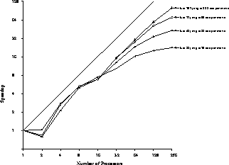
Figure 14.8:
The Speedup of the Parallel Chess Program as a Function of
Machine Size and Search Depth. The results are averaged over a
representative test set of 24 chess positions. The speedup increases
dramatically with search depth, corresponding to the fact that there is
more parallelism available in larger searches. The uppermost curve
corresponds to tournament play-the program runs more than 100 times
faster on 256 nodes as on a single nCUBE node when playing at tournament
speed.
The ``double hump'' shape of the curves is also understood: The location of
the first dip, at 16 processors, is the location at which the chess tree
would like the processor hierarchy to be a one-level hierarchy sometimes, a
two-level hierarchy at other times. We always use a one-level hierarchy for
16 processors, so we are suboptimal here. Perhaps this is an indication that
a more flexible processor allocation scheme could do somewhat better.
Next:
14.3.6 Real-time Graphical Performance
Up:
14.3 Computer Chess
Previous:
14.3.4 Load Balancing
Guy Robinson
Wed Mar 1 10:19:35 EST 1995
14.3.6 Real-time Graphical Performance Monitoring
Next:
14.3.7 Speculation
Up:
14.3 Computer Chess
Previous:
14.3.5 Speedup Measurements
One tool we have found extremely valuable in program development and tuning
is a real-time performance monitor with color-graphics display. Our nCUBE
hardware has a high-resolution color graphics monitor driven by many parallel
connections into the hypercube. This gives sufficient bandwidth to support a
status display from the hypercube processors in real time. Our
performance-monitoring software was written by Rod Morison and is
described in [
Morison:88a
].
The display shows us where in the chess tree each processor is, and it draws
the processor hierarchy as it changes. By watching the graphics screen we
can see load imbalance develop and observe dynamic load balancing as it tries
to cope with the imbalance. The performance monitor gave us the first
evidence that dynamic load balancing was necessary, and it was invaluable in
debugging
and tuning the load balancing code.
Guy Robinson
Wed Mar 1 10:19:35 EST 1995
14.3.7 Speculation
Next:
14.3.8 Summary
Up:
14.3 Computer Chess
Previous:
14.3.6 Real-time Graphical Performance
The best computer chessplayer
of 1990 (Deep
Thought) has reached grandmaster strength. How strong a player can be
built within five years, using today's techniques?
Deep Thought is a chess engine implemented in VLSI
that
searches roughly 500,000 positions per second. The speed of
Chiptest-type engines can probably be increased by about a factor of 30
through design refinements and improvements in fabrication technology.
This factor comes from assuming a speed doubling every year, for five
years. Our own results imply that an additional factor of 250 speedup
due to coarse-grain parallelism is plausible. This is assuming
something like a 1000-processor machine with each processor being an
updated version of Deep Thought. This means that a machine capable of
searching 3.75 billion ( ) positions per
second is not out of the question within five years.
) positions per
second is not out of the question within five years.
Communication times will also need to be improved dramatically over the
nCUBE-1 used. This will entail hardware specialization to the requirements
of chess. How far communication speeds can be scaled and how well the
algorithm can cope with proportionally slower communications are poorly
understood issues.
The relationship between speed and playing strength is well-understood for
ratings below 2500. A naive extrapolation of Thompson's results
[
Thompson:82a
] indicates that a doubling in speed is worth about 40
rating points in the regime above 2500. Thus, this machine would have a
rating somewhere near 3000, which certainly indicates world-class playing
strength.
Of course nobody really knows how such a powerful computer would do against
the best grandmasters. The program would have an extremely unbalanced style
and might well be stymied by the very deep positional play of the world's
best humans. We must not fall prey to the overconfidence which led top
computer scientists to lose consecutive bets to David Levy!
Guy Robinson
Wed Mar 1 10:19:35 EST 1995
14.3.8 Summary
Next:
High-Level Asynchronous Software
Up:
14.3 Computer Chess
Previous:
14.3.7 Speculation
Steve Otto and Ed Felten were the leaders of the chess project and
did the majority of the work. Eric Umland began the project and would
have been a major contributor but for his untimely death. Rod Morison
wrote the opening book code and also developed the parallel graphics
software. Summer students Ken Barish and Rob Fätland contributed
chess expertise and various peripheral programs.
Guy Robinson
Wed Mar 1 10:19:35 EST 1995
High-Level Asynchronous Software
Systems
Next:
15.1 Asynchronous Software Paradigms
Up:
Parallel Computing Works
Previous:
14.3.8 Summary
Guy Robinson
Wed Mar 1 10:19:35 EST 1995
15.1 Asynchronous Software Paradigms
Next:
MOOS II: An
Up:
High-Level Asynchronous Software
Previous:
High-Level Asynchronous Software
There is not now nor will there be a single software paradigm that applies
to all parallel applications. The previous chapters have shown one
surprising fact. At least 90% of all scientific and engineering
computations can be supported by loosely synchronous message-passing
systems, such as CrOS (Express) at a low level and data-parallel
languages such as High Performance Fortran at a higher and somewhat
less general level. The following chapters contain several
different software approaches that sometimes are alternatives for
synchronous and loosely synchronous problems, and sometimes are
designed to tackle more general applications.
Figures
3.11
(a) and
3.11
(b) illustrate two
compound problem
architectures-one
of which the battle management simulation of
Figure
3.11
(b) is discussed in detail in
Sections
18.3
and
18.4
. MOVIE, discussed in
Chapter
17
, and the more ad hoc heterogeneous software
approach described in Section
18.3
are designed as
``software glue'' to integrate many disparate interconnected modules.
Each module may itself be data-parallel. The application of
Figure
3.11
(b) involves signal processing, for which data
parallelism is natural, and linking of satellites, for which a
message-passing system is natural. The integration needed in
Figure
3.11
(a) is of different modules of a complex
design and simulation environment-such as that for a new aircraft or
automobile described in Chapter
19
. We redraw the application
of Figure
3.11
(a) in Figure
15.1
to indicate
that one can view the software infrastructure in this case as forming a
software ``bus'' or backbone into which one can ``plug'' application
modules. This software integration naturally involves an interplay
between parallel and distributed computing. This is graphically shown
in Figure
15.2
, which redisplays Figures
3.10
and
3.11
(a) to better indicate the analogy between a
software network (bus) and a heterogeneous computer network. The
concept of metacomputer
has been coined to describe
the integration of a heterogeneous computer network to perform as a
single system. Thus, we can term the systems in Chapter
17
and Section
18.3
as
metasoftware
systems
, and so on, software for implementing
metaproblems
on
metacomputers.
Figure 15.1:
General Software Structure for Multidisciplinary Analysis and
Design
Figure:
The Mapping of Heterogeneous Problems onto Heterogeneous
Computer Systems combining Figure
3.10
and
Figure
3.11
(a).
The discussion in Chapter
16
shows how different starting
points can lead to similar results. Express, discussed in Chapter
5
,
can be viewed as a flexible (asynchronous) evolution of the original
(loosely) synchronous CrOS message-passing system. Zipcode, described in
Chapter
16
, starts with a basic asynchronous model but
builds on top of it the structure necessary to efficiently represent
loosely synchronous and synchronous problems.
MOOSE, described in the following section, was in some sense a dead
end, but the lessons learned helped the evolution of our later
software as described in Chapter
5
. MOOSE was designed to
replace CrOS but users found it unnecessarily powerful for the
relatively simple (loosely) synchronous problems being tackled by
C P at the time.
The Time Warp operating system described briefly in Section
15.3
is an important software approach to the very difficult asynchronous
event-driven simulations described in Section
14.1
. The
simulations described in Section
18.3
also used this
software approach combined in a heterogeneous environment with our fast,
loosely synchronous system CrOS. This illustrates the need for and
effectiveness of software designed to support a focussed subclass of
problems. The evolution of software support for asynchronous problems
would seem to need a classification with the complete asynchronous
class divided into subclasses for which one can separately generate
appropriate support. The discussions of Sections
14.2
,
14.3
,
15.2
,
15.3
, and
18.3
represent
C P's contributions to this isolation of subclasses with their
needed software. Chapters
16
and
17
represent a
somewhat different approach in developing general software frameworks
which can be tailored to each problem class.
P's contributions to this isolation of subclasses with their
needed software. Chapters
16
and
17
represent a
somewhat different approach in developing general software frameworks
which can be tailored to each problem class.
Next:
MOOS II: An
Up:
High-Level Asynchronous Software
Previous:
High-Level Asynchronous Software
Guy Robinson
Wed Mar 1 10:19:35 EST 1995
MOOS II: An Operating System forDynamic Load Balancing on the iPSC/1
Next:
15.2.1 Design of MOOSE
Up:
High-Level Asynchronous Software
Previous:
15.1 Asynchronous Software Paradigms
Applications involving irregular time behavior or dynamically varying data
structures are difficult to program using the crystalline model or its
variants. Examples are dynamically adaptive grids for studying shock waves in
fluid dynamics, N-body
simulations of gravitating
systems, and artificial intelligence applications, such as chess. The
few applications in this class that have been written typically use
custom designed operating systems and special techniques.
To support applications in this class, we developed a new, general-purpose operating system called MOOSE
for the Mark II hypercube
[
Salmon:88a
], and later wrote an extended version called MOOS II
for the Intel iPSC/1 [
Koller:88b
]. While the MOOSE system was
fairly convenient for some applications, it became available at a time
when the Mark II and iPSC/1 were falling into disuse because of
uncompetitive performance. The iPSC/1 was used for MOOS II for two
reasons: It had the necessary hardware support on the node, and,
because of low performance, it had little production use for scientific
simulation. Thus, we could afford to devote the iPSC/1 to the
``messy'' process of developing a new operating system which rendered
the machine unusable to others for long periods of time. Only one
major application was ever written using MOOSE (Ray tracing,
[
Goldsmith:88a
], mentioned in Section
14.1
[
Salmon:88c
]), and only toy applications were written using
MOOS II. Its main value was therefore as an experiment in operating
system design and some of its features are now incorporated in Express
(Section
5.2
). The lightweight threads pioneered in MOOSE
are central to essentially all new distributed- and shared-memory
computing models-in particular MOVIE, described in
Chapter
17
.
Guy Robinson
Wed Mar 1 10:19:35 EST 1995
15.2.1 Design of MOOSE
Next:
15.2.2 Dynamic Load-Balancing Support
Up:
MOOS II: An
Previous:
MOOS II: An
The user writes a MOOSE program as a large collection of small tasks that
communicate with each other by sending messages through pipes, as shown
in Figure
15.3
. Each task controls a piece of data, so it can
be viewed as an object in the object-oriented sense (hence the name
Multitasking
Object-oriented OS). The tasks and
pipes can be created at any time by any task on any node, so the whole
system is completely dynamic.
Figure 15.3:
An Executing MOOSE Program Is a Dynamic Network (left) of Tasks
Communicating Through FIFO Buffers Called Pipes (right).
The MOOS II extensions allow one to form groups of tasks called teams that
share access to a piece of data. Also, a novel feature of MOOS II is that
teams are relocatable, that is, they can be moved from one node to another
while they are running. This allows one to perform dynamic load balancing if
necessary.
The various subsystems of MOOS II, which together form a complete operating
system and programming environment, are shown in Figure
15.4
.
For convenience, we attempted to preserve a UNIX flavor in the design and
were also able to provide support for debugging
and
performance evaluation because the iPSC/1 hardware has built-in memory
protection. Easy interaction with the host is achieved using
ICubix,
an asynchronous version of Cubix
(Section
5.2
) that gives each task access to the Unix system
calls on the host. The normal C-compilers can be used for programming,
and the only extra utility program required is a binder to link the
user program to the operating system.
Figure 15.4:
Subsystems of the MOOS II Operating System
Despite the increased functionality, the performance of MOOS II on the iPSC/1
turned out to be slightly better than that of Intel's proprietary NX system.
Next:
15.2.2 Dynamic Load-Balancing Support
Up:
MOOS II: An
Previous:
MOOS II: An
Guy Robinson
Wed Mar 1 10:19:35 EST 1995
15.2.2 Dynamic Load-Balancing Support
Next:
15.2.3 What We Learned
Up:
MOOS II: An
Previous:
15.2.1 Design of MOOSE
Our plan was to use MOOS II to study dynamic load balancing
(Chapter
11
), and eventually incorporate a
dynamic load balancer
in the MOOSE system.
However, our first implementation of a dynamic load balancer, along the
lines of [
Fox:86h
], convinced us that dynamic load balancing is a
difficult and many-faceted issue, so the net result was a better
understanding of the subject's complexities rather than a
general-purpose balancer.
The prototype dynamic load balancer worked as shown in
Figure
15.5
and is appropriate for applications where the
number of MOOSE teams in an application is constant. However, the amount of work
performed by individual teams changes slowly with time. A centralized
load manager on node 0 keeps statistics on all the teams in the machine.
At regular intervals, the teams report the amount of computation and
communication they have done since the last report, and the central manager
computes the new load balance. If the balance can be improved significantly,
some teams are relocated to new nodes, and the cycle continues.
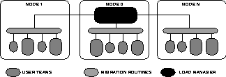
Figure 15.5:
One Simple Load-Balancing Scheme Implemented in MOOS II
This centralized approach is simple and successful in that it relocates
as few teams as possible to maintain the balance; its drawback is
that computing which teams to move becomes a sequential
bottleneck.
For instance, for 256 teams on
16 processors, a simulated annealing
optimization takes about 1.2 seconds on the iPSC/1, while the actual
relocation process only takes about 0.3 seconds, so the method is
limited to applications where load redistribution needs only to be done
every 10 seconds or so. The lesson here is that, to be viable, the
load optimization step itself must be parallelized. The same
conclusion will also hold for any other distributed-memory machine,
since the ratio of computation time to optimization time is fairly
machine-independent.
Next:
15.2.3 What We Learned
Up:
MOOS II: An
Previous:
15.2.1 Design of MOOSE
Guy Robinson
Wed Mar 1 10:19:35 EST 1995
15.2.3 What We Learned
Next:
15.3 Time Warp
Up:
MOOS II: An
Previous:
15.2.2 Dynamic Load-Balancing Support
Aside from finding some new reasons not to use old hardware, we were able to
pinpoint issues worthy of further study, concerning parallel programming in
general and load balancing in particular.
-
In the MOOSE programming style, it is messy and expensive for user tasks
to find out when other groups of tasks have terminated. In our defense, the
same unsolved problem exists in ADA.
-
There are serious ambiguities in the meaning of parallel-file IO for
asynchronous systems like MOOSE, which are exacerbated when tasks can move
from node to node. When writing, does each task have a block in the file,
and if so, how do we correlate tasks with blocks? There are hints that
a hypertext-like system is more suitable than a linear file for parallel
IO, but we were unable to obtain completely satisfactory semantics.
-
It is not clear that there is a general solution to the dynamic load-balancing
problem. The issue may be as resistant to classification as, say,
the general nonlinear PDE problem. A better solution may be to provide
language support so that the programmer can control the load distribution as
part of the program. Existing applications that load-balance successfully
(e.g., chess [
Felten:87a
] in Section
14.3
or the
N-body
solver [
Salmon:89a
] in Section
12.4
)
compute and use load information on the fly in ways that a
general-purpose method could not.
-
As the number of tasks grows,
the amount of load information grows enormously, and we have to be
selective about what we record. The best choice seems to be
application- and machine-dependent.
-
In irregular problems,
having a large number of tasks does not automatically solve the
load-balancing problem. Unforeseen correlations between tasks tend to
appear that confound naive balancing schemes. The load-balancing
problem must be tackled on many scales simultaneously.
Future work will therefore have to focus less on the mechanism of moving
tasks around and more on how to communicate load information between user and
system.
MOOSE was written by John Salmon, Sean Callahan, Jon Flower and Adam Kolawa.
MOOS II was written by Jeff Koller.
The C P references are: [Salmon:88a], [Koller:88a;88b;88d;89a], [Fox:86h].
Next:
15.3 Time Warp
Up:
MOOS II: An
Previous:
15.2.2 Dynamic Load-Balancing Support
Guy Robinson
Wed Mar 1 10:19:35 EST 1995
15.3 Time Warp
Next:
16 The Zipcode Message-Passing
Up:
High-Level Asynchronous Software
Previous:
15.2.3 What We Learned
Discrete-event simulations are among the most expensive of all computational
tasks. With current technology, one sequential execution of a large
simulation can take hours or days of sequential processor time. For example,
many large military simulations take days to complete on standard single
processors. If the model is probabilistic, many executions will be necessary
to determine the output distributions. Nevertheless, many scientific,
engineering, and military projects depend heavily on simulation because
experiments on real systems are too expensive or too unsafe. Therefore, any
technique that speeds up simulations is of great importance.
We designed the Time Warp Operating System (TWOS)
to
address this problem. TWOS is a multiprocessor operating system that
runs parallel discrete-event simulations. We developed TWOS on the
Caltech/JPL Mark III Hypercube. We have since ported it to various
other parallel architectures, including the
Transputer
and a BBN Butterfly GP1000. TWOS is not
intended as a general-purpose multiuser operating system, but rather as
an environment for a single concurrent application (especially a
simulation) in which synchronization is specified using virtual
time
[
Jefferson:85c
].
The innovation that distinguishes TWOS from other operating systems is its
complete commitment to an optimistic style of execution and to processing
rollback
for almost all synchronization. Most
distributed operating systems either cannot handle process rollback at
all or implement it as a rarely used mechanism for special purposes
such as exception handling, deadlock
,
transaction abortion, or fault recovery. But the Time Warp Operating
System embraces rollback as the normal mechanism for process
synchronization, and uses it as often as process blocking is used in
other systems. TWOS contains a simple, general distributed rollback
mechanism capable of undoing or preventing any side effect, direct or
indirect, of an incorrect action. In particular, it is able to control
or undo such troublesome side effects as errors, infinite loops,
I/O,
creation and destruction of processes, asynchronous
message communication, and termination.
TWOS uses an underlying kernel to provide basic message-passing capabilities,
but it is not used for any other purpose. On the Caltech/JPL Mark III
Hypercube, this role was played by
Cubix
,
described in
Section
5.2
. The other facilities of the underlying operating
system are not used because rollback forces a rethinking of almost all
operating system issues, including scheduling, synchronization, message
queueing, flow control, memory management, error handling, I/O, and
commitment. All of these are handled by TWOS. Only the extra work of
implementing a correct message-passing facility prevents TWOS from being
implemented on the bare hardware.
We have been developing TWOS since 1983. It is now an operational system
that includes many advanced features such as dynamic creation and destruction of
objects, dynamic memory management, and dynamic load management. TWOS is
being used by the United States Army's Concept and Analysis Agency to develop
a new generation of theater-level combat simulations. TWOS has also been used
to model parallel processing hardware, computer networks, and biological
systems.
Figure
15.6
shows the performance of TWOS on one simulation
called STB88. This simulation models theater-level combat in central Europe
[
Wieland:89a
]. The graph in Figure
15.6
shows how much
version 2.3 of TWOS was able to speed up this simulation on varying numbers of
nodes of a parallel processor. The speedup shown is relative to running a
sequential simulator on a single node of the same machine used for the TWOS
runs. The sequential simulator uses a splay tree for its event queue. It
never performs rollback, and hence has a lower overhead than TWOS. The
sequential simulator links with exactly the same application code as TWOS. It
is intended to be the fastest possible general-purpose discrete-event
simulator that can handle the same application code as TWOS.
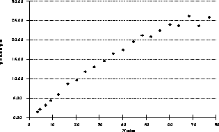
Figure 15.6:
Performance of TWOS on STB88
Figure
15.6
demonstrates that TWOS can run this simulation more
than 25 times faster than running it on the sequential simulator, given
sufficient numbers of nodes. On other applications, even higher speedups are
possible. In certain cases, TWOS has achieved up to 70% of the maximum
theoretical speedup, as determined by critical path analysis.
Research continues on TWOS. Currently, we are investigating dynamic load
management [
Reiher:90a
]. Dynamic load management is important for
TWOS because good speedups generally require careful mapping of a simulation's
constituent objects to processor nodes. If the balance is bad, then the run
is slow. But producing a good static balance takes approximately the same
amount of work as running the simulation on a single node. Dynamic load
management allows TWOS to achieve nearly the same speed with simple mappings
as with careful mappings.
Dynamic load management is an interesting problem for TWOS because the
utilizations of TWOS' nodes are almost always high. TWOS optimistically
performs work whenever work is available, so nodes are rarely idle. On the
other hand, much of the work done by a node may be rolled back, contributing
nothing to completing the computation. Instead of balancing simple
utilization, TWOS balances effective utilization, the proportion of a node's
work that is not rolled back. Use of this metric has produced very good
results.
Future research directions for TWOS include database management, real-time
user interaction with TWOS, and the application of virtual time
synchronization to other types of parallel processing problems.
[
Jefferson:87a
] contains a more complete description of TWOS.
Participants in this project were David Jefferson, Peter Reiher, Brian
Beckman, Frederick Wieland, Mike Di Loreto, Philip Hontalas, John
Wedel, Paul Springer, Leo Blume, Joseph Ruffles, Steven Belenot, Jack
Tupman, Herb Younger, Richard Fujimoto, Kathy Sturdevant, Lawrence
Hawley, Abe Feinberg, Pierre LaRouche, Matt Presley, and Van Warren.
Next:
16 The Zipcode Message-Passing
Up:
High-Level Asynchronous Software
Previous:
15.2.3 What We Learned
Guy Robinson
Wed Mar 1 10:19:35 EST 1995
16 The Zipcode Message-Passing System
Next:
16.1 Overview of Zipcode
Up:
Parallel Computing Works
Previous:
15.3 Time Warp
Guy Robinson
Wed Mar 1 10:19:35 EST 1995
16.1 Overview of Zipcode
Next:
16.2 Low-Level Primitives
Up:
16 The Zipcode Message-Passing
Previous:
16 The Zipcode Message-Passing
Zipcode
is a message-passing system developed
originally by Skjellum, beginning at Caltech in the Summer of 1988
[
Skjellum:90a
], [
Skjellum:91c
], [
Skjellum:92c
] and
[
Skjellum:91a
].
Zipcode
was created to address features
and issues absent in then-existing message-passing systems such as
CrOS/Express, described in Section
5.2
. In particular,
Zipcode
was based on an underlying reactive asynchronous low-level
message-passing system. CrOS was built on top of loosely synchronous
low-level message-passing systems, which reflected C P's initial
hardware and applications. Interestingly, both
Zipcode
and
Express have evolved from their starting to quite similar high-level
functionality. Currently,
Zipcode
continues to serve as a
vehicle to demonstrate high-level message-passing research concepts
and, more importantly, to provide the basis for supporting
vendor-independent scalable concurrent libraries; notably, the
Multicomputer Toolbox
[
Falgout:92a
],
[Skjellum:91b;92a;92d].
The basic assertion of
Zipcode
is that carefully managed,
expressive message-passing is an effective way to program
multicomputers and distributed computers, while low-level message
passing is admittedly both error-prone and difficult.
P's initial
hardware and applications. Interestingly, both
Zipcode
and
Express have evolved from their starting to quite similar high-level
functionality. Currently,
Zipcode
continues to serve as a
vehicle to demonstrate high-level message-passing research concepts
and, more importantly, to provide the basis for supporting
vendor-independent scalable concurrent libraries; notably, the
Multicomputer Toolbox
[
Falgout:92a
],
[Skjellum:91b;92a;92d].
The basic assertion of
Zipcode
is that carefully managed,
expressive message-passing is an effective way to program
multicomputers and distributed computers, while low-level message
passing is admittedly both error-prone and difficult.
The purpose of
Zipcode
is to manage the message-passing process
within parallel codes in an open-ended way. This is done so that
large-scale software can be constructed in a multicomputer application,
with reduced likelihood that software so constructed will conflict in
its dynamic resource use, thereby avoiding potentially hard-to-resolve,
source-level conflicts. Furthermore, the message-passing notations
provided are to reflect the algorithms and data organizations of the
concurrent algorithms, rather than predefined tagging strategies.
Tagging, while generic and easy to understand, proves insufficient to
support manageable application development. Notational abstractions
provide a means for the user to help
Zipcode
make runtime
optimizations when a code runs on systems with specific hardware
features. Abstraction is therefore seen as a means to higher
performance, and notation is seen as a means towards more
understandable, easier-to-develop-and-maintain concurrent software.
Context allocation (see below) provides a ``social contract'' within
which multiple libraries and codes can coexist reasonably. Contexts
are like system-managed ``hypertag''; contexts here are called
``Zipcodes''.
Safety in communication is achieved by
context
control; the
main process data structure is the process list (a collective of
processes that are to communicate). These constructs are handled
dynamically by the system. Contexts are needed so that diverse codes
can be brought together and made to work without the possibility of
message-passing conflicts, and without the need to globalize the
semantic and syntactic issues of message passing contained in each
separate piece of code. For instance, the use and support of
independently conceived concurrent libraries requires separate
communication space, which contexts support. As applications mature,
more contexts are likely to be needed, especially if diverse libraries
are linked into the system, or a number of (possibly overlapping)
process structures are needed to represent various phases of a
calculation. In purely message-passing instances within
Zipcode
, contexts control the flow of messages through a global
messaging resource. In more complex hierarchies, contexts will manage
channel and/or shared-memory blocks in the user program, while the
notation remains message-passing-like to the user. This evolution is
transparent to the user.
Concurrent mathematical libraries are well supported by the definition
of multidimensional, logical-process-grid primitives, as provided by
Zipcode
; one-, two- and three-dimensional grids are currently
supported (grid
mail classes
, also known as virtual topologies).
Grids are used to assign machine-independent naming to the processes
participating in a calculation, with a shape chosen by the user. Such
grids form the basis for higher level data structures that describe how
matrices and vectors are shared across a set of processes, but these
descriptors are external to
Zipcode
. New grids may be aligned
to existing grids to provide nesting, partitioning, and other desired
subsetting of process grids, all done in the machine-independent
notation of the parent grid. The routine
whoami
and associated routines, described in Section
5.2
, provide
this capability in CrOS/Express.
Mail classes
(such as new grid structures) may be
added statically to the system; because code cannot move with data in
extant multicomputers, mail classes have to be enumerated at
compile-time. Because we at present retain a C implementation, rather
than C++, the library must currently be modified explicitly to add new
classes of mail, rather than by inheritance. Fortunately, the
predefined classes (grids, tagged messages) address a number of the
situations we have encountered thus far in practical applications.
Non-mathematically oriented users may conceive of mail classes that we
have not as yet imagined, and which might be application-specific.
Recently, we have evolved the
Zipcode
system to provide
higher level application interfaces to the basic message-passing
contexts and classes of mail. These interfaces allow us to unify the
notions of heterogeneity and non-uniform memory access hierarchy in a
single framework, on a context-by-context basis. For instance, we view
a homogeneous collection of multicomputer nodes as a particular type of
memory hierarchy. We see this unification of heterogeneity and memory
hierarchy in our notation as an important conceptual advance, both for
distributed- and concurrent-computing applications of
Zipcode
.
Mainly, heterogeneity impacts transmission bandwidth
and should not have to be treated as a separate feature in data
transmission, nor should it be explicitly visible in user-defined
application code or algorithms, except perhaps in highly restricted
method definitions, for performance' sake.
For instance, the notations currently provided by
Zipcode
support writing application programs so that the same message-passing
code can map reasonably well to heterogeneous architectures, to those
with shared memory
between subsets of nodes, and
to those which support active-message strategies. Furthermore, it
should be possible to cache limited internode channel resources within
the library, transparent to the user. This is possible because the
gather-send and scatter-receive notations remove message formatting
from the user's control. We provide general gather/scatter
specifications through persistent
invoice
data types. This
notation is available both to C and Fortran programmers. As a side
effect, we provide a clean interface for message passing in the Fortran
environment. If compilers support code inlining and other
optimizations, we are convinced that overheads can be drastically
reduced for systems with lighter communication overheads than
heretofore developed. Cheap dynamic allocation mechanisms also help in
this regard, and are easily attainable. In all cases, the user will
have to map the process lists to processors to take advantage of the
hierarchies, but this can be done systematically using
Zipcode
.
We define message-passing operations on a context-by-context basis
(methods), so that the methods implementing send, receive, combine,
broadcast
, and so on, are potentially different for
each context, reflecting optimizations appropriate to given parts of a
hierarchy (homogeneity, power-of-two, flat shared memory, and so on).
We have to rely on the user to map the problem to take advantage of
such special contexts, but we provide a straightforward mechanism to
take advantage of hierarchy through the gather/scatter notation. When
compilers provide inlining, we will see significant improvements in
performance for lower latency
realizations of the
system. Higher level notation, and context-by-context method
definitions are key to optimizing for memory hierarchy and
heterogeneity. Because the user provides us with information on the
desired operations, rather than instructions on how to do them, we are
able to discover optimizations. Low-level notations cannot hope to
achieve this type of optimization, because they do not expose the
semantic information in their instructions, nor work over process
lists, for which special properties may be asserted (except with
extensive compile-time analysis).
This evolutionary process implies that
Zipcode
has surpassed its
original
Reactive Kernel/Cosmic Environment
platform; it is now
planned that
Zipcode
implementations will be based on one or more of
the following in a given implementation:
-
Hardware-based shared memory (with and/or without an intervening
CE/RK layer),
-
Active-message strategies (cf., [
Eiken:92a
]),
-
Pure message passing (with and/or without an intervening CE/RK layer),
-
Control-network operations definable on process lists (subsets of
processes or processors).
Heterogeneous translation can be by one of several translation
mechanisms. For instance, XDR [
XDR:87a
], ELROS [Branstetter:91a;92a]
or other strategies
(that appropriately balance the work of the sender and recipient in the
translation process as a function of their computational
bandwidth
for such translations). Because
invoices are persistent objects, the possibility of nodal
vectorization of translated objects is possible, using ELROS or other
machine-specific strategies (perhaps user-defined); XDR is not
currently amenable to vectorization. Such translation strategies will
also be held transparent to the user, except when the user chooses to
intervene, by providing a submethod that implements part of an
invoice translation. With this approach, we can take advantage of the
architectures presented at run time, on a context-by-context basis.
Importantly, when a code is moved to a system that does not have
special features (e.g., a purely message-passing system), the
user code's calls to
Zipcode
will compile down to pure
message-passing, whereas the calls compile down to faster schemes
within special hierarchies. This multifaceted approach to implementing
Zipcode
follows its original design philosophy; originally, the
CE/RK primitives upon which
Zipcode
is based
were the cheapest available primitives for system-level message-passing,
and hence the most attractive to build higher level services like
Zipcode
.
Today, vendor operating systems are likely to
provide additional services in the other categories mentioned above
which, if used directly in applications, would prove unportable,
unmanageable, or too low level (like direct use of CE/RK
primitives). If a user needs to optimize a code for a specific
system, he or she works in terms of process lists and contexts to get
desirable mappings from which
Zipcode
can effect runtime optimizations.
The CE/RK primitives (originally central to
Zipcode
)
manage memory as well as message-passing operations. This is an
important feature, carried into the
Zipcode
system, which is
helpful in reducing the number of copies needed to pass a message from
sender to recipient in basic message (hence, less wasted
bandwidth
). In CE/RK the system provides
message space, which is freed upon transmission and allocated upon
receipt. This approach removes the need for complicated strategies
involving asynchronous sends, in which the user has to poll to see when
his or her buffer is once again usable. Since the majority of
transmissions in realistic applications involve a gather before send
(and scatter on receive), rather than block-data transmission, these
semantics provide, on the whole, good notational and performance
benefits, while retaining simplicity.
Zipcode
extends the
concept of the CE/RK-managed messages to include buffered
messages (for global operations) and synchronizations. These three
varieties of primitives make different assumptions about how memory is
allocated (and by whom), and are implemented with the most efficient
available system calls in a given
Zipcode
implementation. In
all cases, actual memory allocation can be effected using lightweight
allocation procedures in efficient implementations, rather than
heavyweight mallocs. Therefore, the dynamic nature of the allocations
need not imply significant performance penalties.
When moving
Zipcode
to a new system, the CE/RK layer will
normally be the first interface provided, with additional interfaces
provided if the hardware's special properties so warrant. In this way,
user codes and libraries will come up to speed quickly, yet attain better
performance as the
Zipcode
port is optimized for the new system.
We see this as a desirable mode of operation, with the highest
initial return on investment.
Next:
16.2 Low-Level Primitives
Up:
16 The Zipcode Message-Passing
Previous:
16 The Zipcode Message-Passing
Guy Robinson
Wed Mar 1 10:19:35 EST 1995
16.2 Low-Level Primitives
Next:
16.2.1 CE/RK Overview
Up:
16 The Zipcode Message-Passing
Previous:
16.1 Overview of Zipcode
Guy Robinson
Wed Mar 1 10:19:35 EST 1995
16.2.1 CE/RK Overview
Next:
16.2.2 Interface with the
Up:
16.2 Low-Level Primitives
Previous:
16.2 Low-Level Primitives
To appreciate the model upon which current
Zipcode
implementations
are built, one needs to understand the scope and expressivity of the
low-level CE/RK system.
Guy Robinson
Wed Mar 1 10:19:35 EST 1995
16.2.2 Interface with the CE/RK system
Next:
16.2.3 CE Functions
Up:
16.2 Low-Level Primitives
Previous:
16.2.1 CE/RK Overview
Implementations of
Zipcode
todate interface to primitives of
the CE/RK, a portable, lightweight multicomputer node
operating system, which provides untyped blocked and unblocked message
passing in a uniform host/node model, including type conversion
primitives for heterogeneous host-node communications. Presently, the
Reactive Kernel is implemented for Intel iPSC/1, iPSC/2,
Sequent
Symmetry, Symult S2010, and Intel iPSC860 Gamma
prototype multicomputers, with emulations provided for the Intel Delta
prototype, Thinking Machines CM-5, and nCUBE/2
6400
machines. Furthermore, Intel provides the CE/RK primitives at the
lowest level (read: highest performance) on its Paragon system. CE/RK
is also emulated on shared-memory computers such as the BBN TC2000 as
well as networks of homogeneous NFS-connected workstations (e.g., Sun
clusters). We see CE/RK primitives as a logical, flexible platform for
our work, and for other message-passing developers, and upon which
higher level layers such as
Zipcode
can be ported. Because
most tagged message-passing systems with restrictive typing semantics
do not provide quite enough receipt selectivity directly to support
Zipcode
, we find it often best to implement untagged primitives
as the interface to which
Zipcode
works. The CE/RK emulations,
built most often on vendor primitives, make use of any available
tagging for bookkeeping purposes, and allow users of a specific vendor
system to mix vendor-specific message passing with CE/RK- or
Zipcode
-based messaging.
One should view the CE/RK system as the default message-space
management system for
Zipcode
(in C++ parlance, default
constructor/new, destructor/free mechanisms), with the understanding
that future implementations of
Zipcode
may prefer to use more
primitive calls (e.g., packet protocols or active messages) to
gain even greater performance. (Alternatively, if Paragon or similar
implementations are very fast, such shortcuts will have commensurately
less impact on performance.) Via the shortcut approach,
Zipcode
analogs of CE/RK calls will become the lowest level
interface of message passing in the system, and become a machine-dependent layer.
Next:
16.2.3 CE Functions
Up:
16.2 Low-Level Primitives
Previous:
16.2.1 CE/RK Overview
Guy Robinson
Wed Mar 1 10:19:35 EST 1995
16.2.3 CE Functions
Next:
CE Programs
Up:
16.2 Low-Level Primitives
Previous:
16.2.2 Interface with the
The
Cosmic Environment
(CE) provides control
for concurrent computation through a ``cube dæmon.'' This resource
manager allows multiple real and emulated concurrent computers to be
space-shared [
Seitz:88a
]. The following functions are provided,
and we emulate these on systems that provide analogous host
functionality (this emulation can be done efficiently on the nCUBE/2,
almost trivially on the Gamma, and not at all on the Delta and CM-5):
-
getmc
gets multicomputer resource by type and size for
space-sharing (also called
getcube
);
-
freemc
frees multicomputer resource currently in use
(also called
freecube
);
-
spawn
spawns one or more node processes to a previously
allocated multicomputer partition;
-
ckill
kills one or more extant processes on a
previously allocated multicomputer partition.
Guy Robinson
Wed Mar 1 10:19:35 EST 1995
CE Programs
Next:
16.2.4 RK Calls
Up:
16.2.3 CE Functions
Previous:
16.2.3 CE Functions
To support
Zipcode
, we normally emulate the
CE functions below. Again, some of these
functions, particularly
getmc()
,
freemc()
,
spawn()
,
and
ckill()
, are not
available on all implementations (for instance, the Delta) and are
restricted to the host program:
-
getmc(char *computer_name, int nnodes)
allocates a multicomputer;
-
freemc(void)
deallocates the allocated multicomputer;
-
spawn(char *prog, int node, int pid, char *state)
spawns
processes on one or more nodes;
-
ckill(int node, int pid)
kills processes on one or more nodes;
-
cosmic_init(void)
starts the environment in a process;
-
cosmic_exit(void)
ends the environment in a process;
-
mynode(void)
returns the current process's logical node; number;
-
mypid(void)
returns the current process's identification
number (pid);
-
nnodes(void)
returns the number of nodes in the
multicomputer allocation;
-
print(char *fmt, ...)
resembles the standard C function
printf()
, except that the output is preceded by
{node,pid}
identification and terminated by a newline, with the output buffer automatically
flushed; and
-
clock()
returns the running nodal clock value in microseconds.
Guy Robinson
Wed Mar 1 10:19:35 EST 1995
16.2.4 RK Calls
Next:
16.2.5 Zipcode Calls
Up:
16.2 Low-Level Primitives
Previous:
CE Programs
The RK calls required by
Zipcode
are as follows:
-
msg = xmalloc(int length)
allocates a message buffer of
length
bytes and
returns a pointer
msg
to it;
-
xfree(char *msg)
deallocates the message buffer pointed to by
msg
;
-
xlength(char *msg)
determines the length (in bytes) of a
previously
allocated or received message
msg
;
-
msg = xrecv()
receives a message without blocking
,
returning a pointer
to the message if a message can be received and NULL if there
is no message queued to the calling process;
-
msg = xrecvb()
blocks until a message can be received and
returns a
pointer to the message;
-
xsend(char *msg, int node, int pid)
sends a message pointed to
by
msg
to the process
pid
on node
node
; and
-
xmsend(char *msg, int count, int *dest)
sends a message
msg
to multiple
destinations specified by the integer array
dest
of length
2*count
in the form
{ node0, pid0, node1, pid1, ...}
.
It is important to note that
xsend()
and
xmsend()
deallocate
the message buffer after sending the message; they are
semantically analogous to
xfree()
. The receive functions
xrecv()
and
xrecvb()
are semantically analogous
to
xmalloc()
.
Zipcode
-based programs are not to call any of these CE or
RK
functions directly. Both message passing and environment control
are represented in
Zipcode
.
Guy Robinson
Wed Mar 1 10:19:35 EST 1995
16.2.5 Zipcode Calls
Next:
Zipcode Class-Independent Calls
Up:
16.2 Low-Level Primitives
Previous:
16.2.4 RK Calls
Guy Robinson
Wed Mar 1 10:19:35 EST 1995
Zipcode Class-Independent Calls
Next:
Mailer Creation
Up:
16.2.5 Zipcode Calls
Previous:
16.2.5 Zipcode Calls
Guy Robinson
Wed Mar 1 10:19:35 EST 1995
Mailer Creation
Next:
Predefined Mailer Classes
Up:
16.2.5 Zipcode Calls
Previous:
Zipcode Class-Independent Calls
Mailers maintain contexts and process lists. All communication
operations use mailers. Mailers are created through a loose
synchronization
between the members of the
proposed mailer's process list. A single process creates the process
list, placing itself first in the list, and initiates the
``mailer-open'' call with this process information; it's called the
``Postmaster'' for the mailer, as initiator. The other participants
receive the process list as part of the synchronization procedure. A
special reactive process, the ``Postmaster General,'' maintains and
distributes zip codes as mailers are opened; essentially the zip code
count is a single location of shared memory.
Below, each class defines an ``open'' function to create its mailer.
Guy Robinson
Wed Mar 1 10:19:35 EST 1995
Predefined Mailer Classes
Next:
Y-Class
Up:
16.2.5 Zipcode Calls
Previous:
Mailer Creation
Guy Robinson
Wed Mar 1 10:19:35 EST 1995
Y-Class
Next:
Z-Class
Up:
Predefined Mailer Classes
Previous:
Predefined Mailer Classes
mail is used mainly for
Zipcode
internal mechanisms. The PO Box information is a single short-integer
type. Global operations are not implemented for this class, because of
its (intentional) simplicity.
Guy Robinson
Wed Mar 1 10:19:35 EST 1995
Z-Class
Next:
L-Class
Up:
Predefined Mailer Classes
Previous:
Y-Class
mail is a general-purpose class. Process names are
abstracted to a single integer (based on position in the process list);
receipt-selectivity is based on that source name. Global operations
are implemented for this class, with analogous calling sequences to the
G2-Class two-dimensional-grid global operations noted below.
Guy Robinson
Wed Mar 1 10:19:35 EST 1995
L-Class
Next:
G1-Class
Up:
Predefined Mailer Classes
Previous:
Z-Class
mail is used to support emulation of typed message
notations such as Intel's NX or PICL [
Geist:92b
]. Process names
are not abstracted, and receipt selectivity is based on the source name
(as
{ node,pid}
pair) plus a type.
We have been able to classify a number of message-passing systems in
[
Skjellum:92c
], though specific differences in sending, and
receiving strategies exist between common tagged-message-passing
systems. In
Zipcode
, we define the L-class, which provides for
receipt selectivity based on message source in unabstracted
{node,pid}
notation, and on a long-integer tag. This
class can be used to define one or more contexts of tagged message
systems, that call the primitives described fully in
[
Skjellum:92b
]. However, and perhaps more interestingly, these
L-class calls can be used to generate wrappers for all the major tagged
message-passing systems. In the
Zipcode
manual we illustrate
how this is done by showing a few of the wrappers for the PICL, NX, and
Vertex system [
Skjellum:92b
]. We also have a long-standing
Zipcode
-based emulation for the Livermore Message Passing System
(LMPS) [
Welcome:92a
].
Furthermore, for each context a user declares, he or she is guaranteed
that the L-class messages will not be mixed up, so that if vendor-style
calls are used in different libraries, then these will not interfere
with other parts of a program. This allows several existing tagged
subroutines or programs to be brought together and face-lifted easily
to work together, without changing tags or seeing when/where the
message passing resources might conflict. In short, this provides a
general means to ensure tagged-message safety, as contemplated in
[
Hart:93a
].
Guy Robinson
Wed Mar 1 10:19:35 EST 1995
G1-Class
Next:
G2-Class
Up:
Predefined Mailer Classes
Previous:
L-Class
mail is a one-dimensional-grid-abstraction class, similar
to Z-Class mail. For brevity, we omit the calls supported by
this class, which are simplified notations of the G2 and G3 classes.
Guy Robinson
Wed Mar 1 10:19:35 EST 1995
G2-Class
Next:
Letter-Generating Primitives
Up:
Predefined Mailer Classes
Previous:
G1-Class
mail is a two-dimensional-grid-abstraction class.
A  grid naming abstraction is attached to the process list;
each process is specified by a
grid naming abstraction is attached to the process list;
each process is specified by a  pair (e.g., in the PO Box).
Through inheritance, row and column mailers are defined in each process
as the appropriate subsets of the two-dimensional grid. This class has
received the most extensive use because of the natural application to
linear algebra and related computations.
pair (e.g., in the PO Box).
Through inheritance, row and column mailers are defined in each process
as the appropriate subsets of the two-dimensional grid. This class has
received the most extensive use because of the natural application to
linear algebra and related computations.
Class-specific primitives for G2-Class mail have been defined for both
higher efficiency and better abstraction. Small-g calls require mailer
specification while big-G calls do not, analogous to the y- and Y-type
calls defined generically above.
Guy Robinson
Wed Mar 1 10:19:35 EST 1995
Letter-Generating Primitives
Next:
Letter-Consuming Primitives
Up:
16.2.5 Zipcode Calls
Previous:
G2-Class
char *letter = g2_Recv(ZIP_MAILER *mailer, int p, int q);
/* unblocked: */
letter = g2_Recvb(ZIP_MAILER *mailer, int p, int q);
/* blocked: */
Guy Robinson
Wed Mar 1 10:19:35 EST 1995
Letter-Consuming Primitives
Next:
G3-Class
Up:
16.2.5 Zipcode Calls
Previous:
Letter-Generating Primitives
void g2_Send(ZIP_MAILER *mailer, char *letter, int p, int q);
Collective operations
combine
,
broadcast
(fanout), and
collapse
(fanin) are defined and
have been highly tuned for this class (see schematics in
[
Skjellum:90c
]).
Combines and fanins are over arbitrary associative-commutative
operators specified by
(*comb_fn)()
. Broadcasts share data of
arbitrary length, assuming all participants know the source. Collapses
combine information assuming all participants know the destination:
int error =
g2_combine(ZIP_MAILER *mailer, /* 2D grid mailer */
void *buffer, /* where result is accumulated */
void (*comb_fn)(), /* operator for combine */
int size /* size of buffer items in bytes */
int items); /* number of buffer items */
error = g2_fanout(ZIP_MAILER *mailer,
void **data, /* data/result */
int *length, /* data length */
int orig_p, int orig_q); /* grid origin of data */
error = g2_fanin(ZIP_MAILER *mailer,
int dest_p, int dest_q, /* destination on grid */
void *buffer, void (*comb_fn)(),
int size, int nitems);
Shorthands provide direct access to row and column children
mailers, tersely providing common communication patterns
within the two-dimensional grid:
g2_row_combine(mailer, buffer, comb_fn, size, items);
g2_col_combine(mailer, buffer, comb_fn, size, items);
g2_row_fanout(mailer, &data, &length, orig_q);
g2_col_fanout(mailer, &data, &length, orig_p;
and
g2_row_fanin(mailer, dest_q, buffer, comb_fn, size, items);
g2_col_fanin(mailer, dest_p, buffer, comb_fn, size, items);
The row/column instructions above compile to G1-grid calls,
since rows and columns of G2 mailers are implemented via
G1 mailers.
G2-Grid mailer creation:
ZIP_MAILER *mailer = g2_grid_open(int *P, int *Q,
ZIP_ADDRESSEES *addr);
Once a G2 grid mailer has been established, it is possible to derive
subgrid mailers by a cooperative call between all the participants in
the original
g2_grid_open()
. In normal applications, this will
result in a set of additional mailers in the postmaster (usually host
program) process, and one additional G2 grid mailer in each node
process. This call allows subgrids to be aligned to the original grid
in reasonably general ways, but requires a basic cartesian subgridding,
in that each subgrid defined must be a rectangular collection of
processes.
The postmaster of the original mailer (often the host process),
initiates the subgrid open request as follows:
/* array of pointer to subgrid mailers: */
ZIP_MAILER **subgrid_mailers =
g2_subgrid_open(ZIP_MAILER *mailer,
/* mailer already opened */
/* for each (p,q) on original grid,
marks its subgrid: */
int (*select_fn)(int p, int q, void *extra),
void *select_extra; /* extra data needed by select_fn() */
int *nsubgrids); /* the number of subgrids created */
while each process in the original
g2_grid_open()
does
a second, standard
g2_grid_open()
:
ZIP_MAILER *subgrid_mailer = g2_grid_open(&P, &Q, NULL);
Each subgrid so created has its own unique contexts of communication.
Finally, it is often necessary to determine the grid shape  , as well as the current process's location on the grid
  , when
using two-dimensional logical grids. Often this information is
housed only in the mailer (though some applications may choose to
duplicate this information). The following calls provide simple access
to these four quantities.
, when
using two-dimensional logical grids. Often this information is
housed only in the mailer (though some applications may choose to
duplicate this information). The following calls provide simple access
to these four quantities.
int p,q, P, Q; ZIP_MAILER *mailer;
/* set variables (P,Q) to grid shape: */
void g2_PQ(ZIP_MAILER *mailer, int P, int Q);
/* set variables (p,q) to grid position: */
void g2_pq(ZIP_MAILER *mailer, int p, int q);
These are the preferred forms for accessing grid information
from G2-Class mailers.
Next:
G3-Class
Up:
16.2.5 Zipcode Calls
Previous:
Letter-Generating Primitives
Guy Robinson
Wed Mar 1 10:19:35 EST 1995
G3-Class
Next:
16.3 High-Level Primitives
Up:
Letter-Consuming Primitives
Previous:
Letter-Consuming Primitives
mail is a three-dimensional-grid-abstraction
class. A  grid naming abstraction is attached to the
process list, analogously to the G2-Class two-dimensional-grid
primitives. This class is interesting for problems where there are
three logical ``axes'' of concurrency. Children of a G3 mailer are G2
mailers representing planes within the three-dimensional grid.
Operations analogous to the two-dimensional case have been extended to
the three-dimensional grid case and are not detailed here (see
[Skjellum:92b;c]).
grid naming abstraction is attached to the
process list, analogously to the G2-Class two-dimensional-grid
primitives. This class is interesting for problems where there are
three logical ``axes'' of concurrency. Children of a G3 mailer are G2
mailers representing planes within the three-dimensional grid.
Operations analogous to the two-dimensional case have been extended to
the three-dimensional grid case and are not detailed here (see
[Skjellum:92b;c]).
Shorthands provide access to the PQ-plane, QR-plane, and PR-plane
children to which G2 grid operations may be applied, as above.
ZIP_MAILER *mailer; /* 3D grid mailer */
ZIP_MAILER *PQ_plane_mailer, QR_plane_mailer, PR_plane_mailer;
PQ_plane_mailer = g3_PQ_plane(mailer);
QR_plane_mailer = g3_QR_plane(mailer);
PR_plane_mailer = g3_PR_plane(mailer);
Guy Robinson
Wed Mar 1 10:19:35 EST 1995
16.3 High-Level Primitives
Next:
16.3.1 Invoices
Up:
16 The Zipcode Message-Passing
Previous:
G3-Class
In order to facilitate easier use and the possibility of heterogeneous
parallel computers,
Zipcode
provides a mechanism to pack and unpack
buffers and letters. Buffers are unstructured arrays of data provided
by the user; they are applicable with buffer-oriented
Zipcode
commands.
Letters are unstructured arrays of data provided by
Zipcode
based on
user specification; they are tied to specific mail contexts and are
dynamically allocated and freed.
Pack (gather) and unpack (scatter) are implemented with the use of
Zip_Invoices
. The analogy is taken from invoices or packing slips used
to specify the contents of a postal package. An invoice
informs
Zipcode
what variables are to be associated with a
communication operation or communication buffer.
This invoice is subsequently used when
zip_pack()
(
zip_unpack()
) is called to copy items from the variables specified
into (out of) the communication buffer space to be sent (received); this
implements gather-on-send- and scatter-on-receive-type semantics.
In a heterogeneous environment, pack/unpacking will allow data
conversions to take place without user intervention. Users who code
with
zip_pack()
/
zip_unpack()
will have codes that are
guaranteed to work in heterogeneous implementations of
Zipcode
.
Guy Robinson
Wed Mar 1 10:19:35 EST 1995
16.3.1 Invoices
Next:
16.3.2 Packing and Unpacking
Up:
16.3 High-Level Primitives
Previous:
16.3 High-Level Primitives
The
zip_new_invoice()
call creates new invoices:
voidzip_new_invoice(Zip\_invoice const char *format, va_list ap)
The call
zip_new_invoice()
creates an invoice (
**inv
),
while taking a variable number of arguments, starting with a format
string (
format
) similar to the commonly used
printf()
strings. The format string contains one or more conversion
specifications. A conversion specification is introduced by a percent
sign (``%'') and is followed by:
-
a positive integer indicating the number of items to convert,
or a ``*'' or ``&'' indicating argument-list specification of
an integer expression or address (see below). If no integer is
specified the default is one item.
-
an optional stride factor indicated by a ``.'' followed by a
positive integer indicating the stride; optionally a ``*'' or ``&''
may be specified, signifying argument-list specification of an integer
expression or address (see below). If no stride is specified the
default is one.
-
an optional ``-'' character indicating that the indicated space
is to be reserved but not packed (ignore-space option).
-
a character specifying an internal type or a string indicating a user type.
For both the number of items to convert and stride, ``*'' or ``&'' can
replace the hard-coded integer. If `*' is used, then the next argument
in the argument list is used as an integer expression specifying the
size of the conversion (or stride). Both the number of items to
convert and the stride factor can be indirected by using ``&'' instead of an
integer. The ``&'' indicates that a pointer to an integer should be
stored, which will address the size of the invoice item (or stride)
when it is packed. When ``&'' is used, the size is not evaluated
immediately but is deferred until the actual packing of the data
occurs. The ``&'' indirection consequently allows variable-size invoices to
be constructed at runtime; we call this feature
deferred sizing
. The
``*'' allows the size of an invoice item (or stride) to be specified at
run time.
One must be cautious of the scope of C variables when using ``&.''
For example, it is improper to create an invoice in a subroutine that has
a local variable as a stride factor and then attempt to pass this
invoice out and use it elsewhere, since the stride factor points at a
variable that is no longer in scope. Unpredictable things will
happen if this is attempted.
The single character types that are supported are as follows:
``c'' character,
``s'' short,
``i'' int,
``l'' long,
``f'' float, and
``d'' double.
For each conversion specification, a pointer to an array of
that type must be passed as an argument.
User-defined types may be added to the system to ease the packing of
complicated data structures. An extra field (for passing whatever the
user wants) may be passed to the conversion routines by adding ``(*)'' to
the end of the user-type name. The ``-'' character can be used to skip
space so that one can selectively push/pull things out of a letter.
This allows for unpacking part of a letter and then unpacking the rest
based on the part unpacked.
The following code would pack variable
i
followed by elements  of the
double_array
.
of the
double_array
.
/* Example 1 */
ZIP_MAILER *mlr;
char *letter;
...
Zip_Invoice*invoice;
int i = 20;
double double_array[20];
zip_new_invoice(``*invoice,%i%10.2d'', &i, double_array);
...
/* use the invoice (see below) */
letter = zip_malloc(mlr, zip_sizeof_invoice(mlr, invoice));
length = zip_pack(mlr, invoice, ZIP_LETTER,
&letter, ZIP_IGNORE);
if(length == -1) /* an error occurred */
...
The second example is a variant of the first. The first pack call
is the same, while the second packs the first five elements of the
double_array
.
/* Example 2 */
int len = 10, stride = 2;
zip_new_invoice(``*invoice,%i%&.&d'', &i, &len, &stride,
double_array);
/* use the invoice */
letter = zip_malloc(mlr, zip_sizeof_invoice(mlr, invoice));
length = zip_pack(mlr, invoice, ZIP_LETTER, &letter,
ZIP_IGNORE);
...
len = 5; /* set the length and stride for this use
of the invoice */
stride = 1;
/* use the invoice */
letter = zip_malloc(mlr, zip_sizeof_invoice(mlr, invoice));
length = zip_pack(mlr, invoice, ZIP_LETTER, &letter,
ZIP_IGNORE);
If a user-defined type
matrix
has been added to the
system to pack matrix structures, then the following example shows how
matrix
-type data can be used in an invoice declaration. See also
below on how to add a user-defined type.
/* Example 3 */
struct matrix M; /* some user-defined type */
int i;
Extra extra; /* contains some special info on packing a */
/* `matrix'; often this will not be needed, */
/* but this feature is provided for */
/* flexibility */
zip_new_invoice(``*invoice,%i%matrix(*)%20d'', &i, &M,
&extra, double_array);
At times it might be useful to know the size (in bytes) that is needed to
hold the variables specified by an invoice.
zip_sizeof_invoice
returns the
size (in bytes) that the invoice will occupy when packed. We have
already used this in several examples above.
int zip_sizeof_invoice(ZIP_MAILER *mailer, Zip_Invoice *inv)
To delete an existing invoice when there is no more need for it use
zip_free_invoice()
:
void zip_free_invoice(Zip_Invoice **inv)
This will free up the specified invoice and set
*inv = NULL
to help flag accidental access.
User-defined types for pack and unpack routines are defined
using a registry mechanism provided by
Zipcode
.
int zip_register_invoice_type(char *name, Method *in, Method
*out, Method *len, Method *align)
The structure
Method
is a composite of a pointer-to-function,
and additional state information for a function call. The details
of
Method
declarations are beyond the scope of this presentation.
In the above,
name
is the user-defined name for the auxiliary
type. User-defined names follow the ANSI standard for C identifiers.
They begin with a nondigit (characters ``A'' through ``Z,'' ``a'' through
``z,'' and the underscore ``_''), followed by one or more nondigits or
digits. User-defined type names currently have global scope so beware
of name conflicts. User-defined types cannot be the same as one of the
built-in types specified above. The
in
,
out
,
len
, and
align
are the
Methods
used to pack/unpack the user-defined
type. They must have the following parameter lists
int in(ZIP_MAILER *mailer, void *SRC="http://www.netlib.org/utk/lsi/pcwLSI/text/http://www.netlib.org/utk/lsi/pcwLSI/text/node387.html">
Next:
16.3.2 Packing and Unpacking
Up:
16.3 High-Level Primitives
Previous:
16.3 High-Level Primitives
Guy Robinson
Wed Mar 1 10:19:35 EST 1995
16.3.2 Packing and Unpacking
Next:
16.3.3 The Packed-Message Functions
Up:
16.3 High-Level Primitives
Previous:
16.3.1 Invoices
Packing is done when one wishes to copy the variables into the communications
buffer space prior to transmission; to access the contents of a packed
buffer, one must unpack it first.
int zip_pack(ZIP_MAILER *mailer, Zip_Invoice *inv,
int buffer_type, char **ptr, int len)
This command packs the invoice. The meaning of
buffer_type
is either
``
ZIP_BUFFER
'' or
``
ZIP_LETTER
,'' indicating whether we are packing into a buffer (say for a
combine or fanout) or a letter (for sends/receives).
If one is packing a buffer and has preallocated the buffer space, then
len
must be set to the size of this allocated buffer space. If
the invoice is too large to fit in this buffer space, an error occurs.
By specifying
*ptr = NULL
and
len = ZIP_IGNORE
, the pack
routine will allocate the space for the buffer based on the size of the
invoice to be packed. Alternatively, if a preallocated letter is
being packed, then pack will fill in the letter by using the
invoice. If the letter provided is not large enough, then an error will
occur. If no preallocated letter is available, the pack routine can create
one automatically, provided
*ptr = NULL
. Note that
len
is
ignored when letters are involved, as the size of letters can be
determined with
Zip_length()
;
len
should always be
ZIP_IGNORE
when packing letters. For either case,
zip_pack()
returns the number of bytes that the data from the invoice occupies
in the communication space (letter or buffer).
To unpack a letter, use
int zip_unpack(ZIP_MAILER *mailer, Zip_Invoice *inv,
int buffer_type, char *ptr)
As in
zip_pack()
,
inv
is the invoice to unpack. The
buffer_type
parameter indicates the type of communication space being
used; that is, whether we are unpacking a letter (
buffer_type =
ZIP_LETTER
) or a buffer (
buffer_type = ZIP_BUFFER
). The
parameter
ptr
is a pointer to the communication space. Unlike
zip_pack()
, we pass a pointer to the communication space to
zip_unpack()
, not a pointer to a pointer. The communication space
must be freed by the caller after it is unpacked.
Next:
16.3.3 The Packed-Message Functions
Up:
16.3 High-Level Primitives
Previous:
16.3.1 Invoices
Guy Robinson
Wed Mar 1 10:19:35 EST 1995
16.3.3 The Packed-Message Functions
Next:
16.3.4 Fortran Interface
Up:
16.3 High-Level Primitives
Previous:
16.3.2 Packing and Unpacking
As may be apparent, many packs are followed almost immediately by sends,
while corresponding receives are followed closely by unpacks. Not only
is this notationally somewhat tedious, but it also limits the
optimizations that can be done by
Zipcode
. To create a more
flexible system,
Zipcode
provides the capability to do both the
pack and communications in a single call. For instance,
g3_pack_send(ZIP_MAILER *g3mailer, int d1, d2, d3,
Zip_Invoice
*invoice)
takes care of creating the letter, packing the invoice, and
sending it to grid location specified by
{d1,d2,d3}
. Whenever
possible, use pack_send-style routines, as they will generally be more
run time optimizable than pack calls followed by send calls.
Packed versions of collective operations are also provided. Here is
the specific syntax for the G2, two-dimensional-grid pack combine:
int g2_pack_combine(ZIP_MAILER *g2mlr, Zip_Invoice *invoice,
void (*func()) )
Guy Robinson
Wed Mar 1 10:19:35 EST 1995
16.3.4 Fortran Interface
Next:
16.4 Details of Execution
Up:
16.3 High-Level Primitives
Previous:
16.3.3 The Packed-Message Functions
The Fortran (F77) interface is provided, but certain features have
necessarily been omitted (awaiting Fortran 90). The syntax is
different since there are no pointers in F77. There are no
user-defined types provided in the Fortran interface as Fortran does
not provide structures. Once Fortran 90 has been adopted, user-defined
types will likely appear in the Fortran interface.
Since Fortran does not allow variable argument functions, the
construction of invoices differs from that of the C interface. An
invoice is built up over several function calls, each one specifying
the next field in the invoice.
C Example 1F
integer mailer
integer letter
...
integer invoice
integer i, length
double double_array(20)
call ZIP_INV_NEW(invoice)
call ZIP_INV_ADD_INT(invoice, i, 1, 1, .false, .false.)
call ZIP_INV_ADD_DBLE(invoice, double_array, 10, 2,
.false., .false.)
C use the invoice
CALL ZIP_SIZEOF_INVOICE(mailer, invoice, length)
CALL YMALLOC(mailer, length, letter)
CALL ZIP_PACK(mailer, invoice, ZIP_LETTER, letter,
ZIP_IGNORE, length)
if(length .eq. -1) then
C an error occurred
...
The above example packs the same invoice that Example 1 does
in C. The last two arguments to
ZIP_INV_ADD_INT()
and
ZIP_INV_ADD_DBLE()
are the ``ignore-space'' and ``deferred-sizing''
logicals, respectively, to be explained via examples below. They
also appear in the C syntax, but as part of the argument string via
special characters.
C Example 2F
integer invoice
integer i, len, stride
DOUBLE double_array(20)
i = 20
len = 10
stride = 2
call ZIP_INV_NEW(invoice)
call ZIP_INV_ADD_INT(invoice, i, 1, 1, .false.,
.false.)
C
C The .true. argument invokes deferred sizing of the data:
call ZIP_INV_ADD_DBLE(invoice, double_array, len,
stride, .false., .true.)
C pack or unpack call is made...
len = 5
stride = 1
C pack or unpack call is made...
This example performs the same work the C Example 2 did. To
ignore space in a pack or unpack call, the ignore-space logical is
set true. For instance:
call ZIP_INV_ADD_INT(invoice, 1, 1, .true., .false.)
To ignore space and use deferred-sizing evaluation, both flags are
set true:
call ZIP_INV_ADD_INT(invoice, len, stride, .true., .true.)
Other
Zipcode
calls are very similar in Fortran to the C versions.
A preprocessor is used to create some definitions for use by the
Fortran programmer.
The following conventions are followed in the Fortran interface.
-
No functions. This avoids some problems on various machines
with returning C values to Fortran code. Return values from
C routines are passed as an extra argument to the Fortran interface.
-
All items that are pointers in C are declared in Fortran as
type
integer
.
A few other minor changes appear because of case-sensitivity issues.
See [
Skjellum:92b
] for the definitive list.
Guy Robinson
Wed Mar 1 10:19:35 EST 1995
16.4 Details of Execution
Next:
16.4.1 Initialization/Termination
Up:
16 The Zipcode Message-Passing
Previous:
16.3.4 Fortran Interface
In this section, we cover the initialization and termination
protocols, and discuss how to get node processes spawned in
the
Zipcode
model of multicomputer programming. Within
this model, the user is not allowed to call CE/RK functions directly.
Guy Robinson
Wed Mar 1 10:19:35 EST 1995
16.4.1 Initialization/Termination
Next:
16.4.2 Process Creation/Destruction
Up:
16.4 Details of Execution
Previous:
16.4 Details of Execution
Each host program and node program must call the appropriate
initialization function to initialize
Zipcode
for their
process:
int error = Zip_init(void);
/* assume default mode for initialization */
error = Zip_global_init(void);
/* assume a simpler host-master model */
void zip_exit(void);
/* terminate Zipcode session */
Guy Robinson
Wed Mar 1 10:19:35 EST 1995
16.4.2 Process Creation/Destruction
Next:
16.5 Conclusions
Up:
16.4 Details of Execution
Previous:
16.4.1 Initialization/Termination
The basic mailer manipulation commands (such as
g1_grid_open()
)
require the specification of process lists, currently as ordered pairs
of nodes and process IDs packaged within a
ZIP_ADDRESSEES
structure. For application convenience, we supply optional commands to
support the creation of such collections. One common collection is a
cohort,
a set of processes with the same process ID,
distributed across a number of nodes. A cohort is often used to
formulate a single-program, multiple-data (SPMD) calculation.
Cohort list creation:
ZIP_ADDRESSEES *addressees =
zip_new_cohort(int N,
/* number of processes involved */
int node_bias,
/* node number of zeroth entry in list */
int cohort_pid,
/* process ID of entire collection of processes */
int host_flag);
/* flags whether host process participates */
Additionally, we provide a
Zipcode
-level spawn mechanism:
int result = zip_spawn(
char *prog_name,
/* ASCII name of program to spawn */
ZIP_ADDRESSEES *addressees,
/* addressee list to spawn */
void *state,
/* future expansion */
int pm_flag);
/* flags if program is spawned on zeroth
addressee */
where
result
is nonzero on failure. Most implementations
require that this spawning function be effected in the host process,
although the original CE/R system did not make this restriction. A
compatible
zip_kill()
is also defined:
result = zip_kill(addressees);
With the addition of these functions,
Zipcode
specifies an
entire programming environment that can be completely divorced, if
desired, from its original foundations in the CE/RK. This is possible
so long as one can emulate appropriate CE/RK functions for
Zipcode
to use. This has been accomplished in release 2.0 of
nCUBE's 6400 system software, for instance.
Guy Robinson
Wed Mar 1 10:19:35 EST 1995
16.5 Conclusions
Next:
MOVIE - Multitasking
Up:
16 The Zipcode Message-Passing
Previous:
16.4.2 Process Creation/Destruction
Zipcode
currently provides portable message-passing capability
on a number of multicomputers. It also works on homogeneous networks
of workstations and will soon be supported on heterogeneous networks
and for heterogeneous multicomputers, when such systems are created.
The key benefits of
Zipcode
are its ability to work over
process lists designated by the user, to define separate contexts of
communication so that message-passing complexity can be managed, and to
allow different notations of message-passing appropriate to the
concurrent algorithms being implemented. Tagged message passing is
seen as a special case of the notations supported by
Zipcode
.
We see notational abstraction as helpful in dealing with issues of
non-uniform memory access hierarchy and heterogeneity in multicomputers
and distributed computers. Abstraction is a way to help
Zipcode
find additional runtime optimizations, rather than a tacit
source of inefficiency. We believe that
Zipcode
implementations will be competitive in performance to tagged message
systems whenever vendors make low-level access to their hardware and
system calls available to us during our implementation phase.
Guy Robinson
Wed Mar 1 10:19:35 EST 1995
MOVIE - Multitasking Object-oriented Visual Interactive
Environment
Next:
17.1 Introduction
Up:
Parallel Computing Works
Previous:
16.5 Conclusions
Guy Robinson
Wed Mar 1 10:19:35 EST 1995
17.1 Introduction
Next:
17.1.1 The Beginning
Up:
MOVIE - Multitasking
Previous:
MOVIE - Multitasking
Guy Robinson
Wed Mar 1 10:19:35 EST 1995
17.1.1 The Beginning
Next:
17.1.2 Towards the MOVIE
Up:
17.1 Introduction
Previous:
17.1 Introduction
The software system described here-
MOVIE
(Multitasking
Object-oriented Visual Interactive Environment)-is
the most
sophisticated developed by C P. Indeed, it is sufficiently complicated
that the project led by Wojtek Furmanski didn't finish the first
prototype until two years after the end of C
P. Indeed, it is sufficiently complicated
that the project led by Wojtek Furmanski didn't finish the first
prototype until two years after the end of C P and Furmanski's move
to Syracuse. MOVIE is designed to address the general
compound
problem class introduced in Section
3.6
and illustrated in
Chapter
18
. Sections
17.3
and
17.2.10
describe current and potential MOVIE applications, and so provide an
interesting discussion of many examples of this complex problem class.
MOVIE is a new software system, integrating High Performance Computing
(HPC) with the Open Systems standards for graphics and networking. The
system was designed and prototyped by Furmanski at Caltech within the
Caltech Concurrent Computation Program and it is currently in the
advanced implementation stage at Northeast Parallel Architectures
Center (NPAC), Syracuse University [
Furmanski:93a
]. The MOVIE System
is structured as a multiserver network of interpreters of the high-level
object-oriented programming language MovieScript. MovieScript derives
from PostScript
and extends it in the C++ syntax-based,
object-oriented, interpreted style towards high-performance computing,
three-dimensional graphics, and general-purpose high-level communication
protocol for distributed and MIMD-parallel computing. The present
paper describes the overall design of the system with the focus on the
HPC component and it discusses in more detail one current application
(Terrain Map Understanding) and one planned application area (Virtual
Reality).
P and Furmanski's move
to Syracuse. MOVIE is designed to address the general
compound
problem class introduced in Section
3.6
and illustrated in
Chapter
18
. Sections
17.3
and
17.2.10
describe current and potential MOVIE applications, and so provide an
interesting discussion of many examples of this complex problem class.
MOVIE is a new software system, integrating High Performance Computing
(HPC) with the Open Systems standards for graphics and networking. The
system was designed and prototyped by Furmanski at Caltech within the
Caltech Concurrent Computation Program and it is currently in the
advanced implementation stage at Northeast Parallel Architectures
Center (NPAC), Syracuse University [
Furmanski:93a
]. The MOVIE System
is structured as a multiserver network of interpreters of the high-level
object-oriented programming language MovieScript. MovieScript derives
from PostScript
and extends it in the C++ syntax-based,
object-oriented, interpreted style towards high-performance computing,
three-dimensional graphics, and general-purpose high-level communication
protocol for distributed and MIMD-parallel computing. The present
paper describes the overall design of the system with the focus on the
HPC component and it discusses in more detail one current application
(Terrain Map Understanding) and one planned application area (Virtual
Reality).
The concept of the MOVIE System emerged in a series of computational
experiments with various software models and hardware environments,
performed by Furmanski during the last few years. His attitude was that
of a computational scientist who tries to find the shortest path
towards a functional (HPC) environment which would be both dynamic enough
to fully utilize the hardware and software technology advances and
stable enough to support reusable programming, resulting in extendible,
backward-compatible and integrable application software.
MOVIE concepts derive from the computational science research within
C P, such as optimal communication [
Fox:88h
] and load-balancing
[
Fox:88e
] algorithms for loosely synchronous problems and, in the
application sector, matrix algebra [
Furmanski:88b
], neural
network
[
Nelson:89a
], and machine vision
[
Furmanski:88c
] algorithms. As a next step, we started to develop
the high-performance software environment for neural networks and
machine vision and we realized that the full model in such areas must
go beyond the regular HPC domain. New required components included
dynamic interactive Graphical User Interfaces (GUI), support for
irregular, dynamic computing which emerges, for example, in higher,
AI-based layers of machine vision, and support for system integration
in the heterogeneous computational model involving diverse components
such as regular massively parallel image processing
and irregular, symbolic expert system techniques. This
complex structure-a ``system of systems''-is typical of the
compound problem class.
P, such as optimal communication [
Fox:88h
] and load-balancing
[
Fox:88e
] algorithms for loosely synchronous problems and, in the
application sector, matrix algebra [
Furmanski:88b
], neural
network
[
Nelson:89a
], and machine vision
[
Furmanski:88c
] algorithms. As a next step, we started to develop
the high-performance software environment for neural networks and
machine vision and we realized that the full model in such areas must
go beyond the regular HPC domain. New required components included
dynamic interactive Graphical User Interfaces (GUI), support for
irregular, dynamic computing which emerges, for example, in higher,
AI-based layers of machine vision, and support for system integration
in the heterogeneous computational model involving diverse components
such as regular massively parallel image processing
and irregular, symbolic expert system techniques. This
complex structure-a ``system of systems''-is typical of the
compound problem class.
Furmanski's work decoupled therefore for some time from the main
C P/NPAC thrust and, assuming tentatively that we ``understand'' the
regular HPC components, he followed an independent exploratory route,
making a series of computational experiments and identifying components
of the ``next-step'' broader model for HPC, which would integrate all
elements discussed above.
P/NPAC thrust and, assuming tentatively that we ``understand'' the
regular HPC components, he followed an independent exploratory route,
making a series of computational experiments and identifying components
of the ``next-step'' broader model for HPC, which would integrate all
elements discussed above.
Next:
17.1.2 Towards the MOVIE
Up:
17.1 Introduction
Previous:
17.1 Introduction
Guy Robinson
Wed Mar 1 10:19:35 EST 1995
17.1.2 Towards the MOVIE System
Next:
17.1.3 Current Status and
Up:
17.1 Introduction
Previous:
17.1.1 The Beginning
The communication and load-balancing algorithms were implemented on
Caltech/JPL hypercube Mark II. The need for interactive GUIs emerged for
the first time during our work on parallel implementation of a
neurophysiological model for olfactory cortex
[
Furmanski:87a
] and, in the next, step, in the machine vision
research [
Furmanski:88c
]. At that time (1988), we were using the
nCUBE1 system at C P and also the ``personal hypercube'' system
based on IBM AT under XENIX with the 4-node nCUBE1 add-on board. The
graphics support in the latter environment was nonexistent and we
constructed from scratch the GUI system based on the interpreted
language
g
[
Furmanski:88a
], custom designed and coupled with the
regular parallel computing software components. The language
g
was
80286 assembly-coded and XENIX kernel-based and hence very fast.
However, it couldn't be ported anywhere beyond this environment, which
clearly became obsolete before the
g
-based implementation work was
even fully completed. Some design concepts and implementation
techniques from this first experiment survived and are now part of the
MOVIE System, but the major lesson learned was that GUIs for HPC must
be based on portable graphics standards rather than on custom-made or
vendor-specific models.
P and also the ``personal hypercube'' system
based on IBM AT under XENIX with the 4-node nCUBE1 add-on board. The
graphics support in the latter environment was nonexistent and we
constructed from scratch the GUI system based on the interpreted
language
g
[
Furmanski:88a
], custom designed and coupled with the
regular parallel computing software components. The language
g
was
80286 assembly-coded and XENIX kernel-based and hence very fast.
However, it couldn't be ported anywhere beyond this environment, which
clearly became obsolete before the
g
-based implementation work was
even fully completed. Some design concepts and implementation
techniques from this first experiment survived and are now part of the
MOVIE System, but the major lesson learned was that GUIs for HPC must
be based on portable graphics standards rather than on custom-made or
vendor-specific models.
It was at about the same time (late 1980s) that the major multivendor
effort started towards standardizing computer graphics in the UNIX
environment. We were participating actively in this process, experimenting
with subsequent models such as SunView, X10, X11, NeWS, XView, OpenLook,
Motif, DPS, and finally PHIGS/PEX/GL. It was very difficult to build a
stable graphics-intensive system for HPC during the period of the last
four years, when the standardization efforts were competing with the
vendor-specific customization efforts. However, certain generic concepts
and required features of such a system gradually started to emerge in
the course of my experiments with subsequent standard candidates.
For example, it became clear, with the onset of network-extensible
server-based graphics models such as X or NeWS, that any solid HPC
environment must include the distributing computing model as well and to
unify it with the SIMD- and MIMD-parallel models. Also, to cope with
portability issues in the emerging heterogeneous HPC environments, such a
system must include appropriate high-level software abstraction layers,
supporting Virtual Machine-based
techniques.
A network of compute servers, tightly/loosely coupled in
MIMD-parallel/distributed mode, with each server following the
high-level Virtual Machine design, appeared to be the natural overall
software architecture. Modern software techniques such as preemptive
multithreading and object orientation are required to assure
appropriate dynamics and functionality of such a server in diverse
tasks involving graphics, computation, and communication. Among the
emerging standards, the design closest to the above specification was
offered by the NeWS
(Network-extensible Window System)
[
Gosling:89a
] server, developed by Sun. Following NeWS ideas, we
adopted PostScript [
Adobe:87a
] syntax for the server language
design, extending it appropriately to support object-oriented
techniques and enhancing substantially its functionality towards the
HPC domain.
The resulting system was called MOVIE, due both to its adequate acronym
and its stress on the relevance of interactive graphics in the system
design. The server language, integrating computation, graphics, and
communication, was called MovieScript. The first implementation of the
MOVIE Server was done at Caltech [
Furmanski:89d
] on a Sun workstation
and then the system was ported to the DEC environment at Syracuse University
[
Furmanski:90b
]. Here, we learned about virtual reality
[
Furmanski:91g
] which we now consider the ultimate GUI
model for MOVIE, ``closing'' the system design. In the fall of 1991, the
MOVIE group was formed and the ``individual researcher'' period of the
system development is now followed by the team development period
[
Furmanski:93a
].
Next:
17.1.3 Current Status and
Up:
17.1 Introduction
Previous:
17.1.1 The Beginning
Guy Robinson
Wed Mar 1 10:19:35 EST 1995
17.1.3 Current Status and Outlook
Next:
17.2 System Overview
Up:
17.1 Introduction
Previous:
17.1.2 Towards the MOVIE
Currently, MOVIE is in the advanced design and development process,
organized as a sequence of internal prereleases of the system code and
documentation. At the time of preparing this document (April 1992),
MOVIE 0.4 has been released internally at NPAC. The associated
technical documentation now contains manual drafts [Furmanski:92a;92b]
and some 25 internal
reports (about 700 pages total). The current total size of the MOVIE
code, including source, binaries, and custom CASE tools, is on the
order of 40 Mb. Both documentation and code will evolve during the
next months towards the first external release MOVIE 1.0, planned for
the fall 1993. MOVIE 1.0 will be associated with the set of
reference/programming manual pairs for all basic system components,
discussed later in this paper (MetaShell, MOVIE Server, MovieScript).
Starting from MOVIE 1.0, we intend to provide user support, assure
backward compatibility, and initiate a series of MOVIE application
projects.
This paper discusses the MOVIE System and is considered as a summary of
the design and prototype development stage (Section
17.2
).
It also contains a brief description of the current status and the
planned near-term applications. A more complete description can be
found in [
Furmanski:93a
] (see also [Furmanski:93b;93d]
for recent overview
reports). Here we concentrate on one current application-Terrain Map
Understanding (Section
17.3
) (see also [
Cheng:92a
]) and on
one planned application area-virtual reality (Section
17.4
)
(see [
Furmanski:92g
] for an overview and [Furmanski:93c;93e;93f]
for the current status).
Guy Robinson
Wed Mar 1 10:19:35 EST 1995
17.2 System Overview
Next:
17.2.1 The MOVIE System
Up:
MOVIE - Multitasking
Previous:
17.1.3 Current Status and
Guy Robinson
Wed Mar 1 10:19:35 EST 1995
17.2.1 The MOVIE System in a Nutshell
Next:
17.2.2 MovieScript as Virtual
Up:
17.2 System Overview
Previous:
17.2 System Overview
MOVIE System is a network of MOVIE servers. MOVIE Server is an
interpreter of MovieScript. MovieScript is a high-level
object-oriented programming language derived from PostScript.
PostScript is embedded in the larger language model of MovieScript.
This includes new types and operators as well as syntax extension
towards the C++ style object-oriented model with dynamic binding and
multiple inheritance. MOVIE Server is based on the custom-made
high-performance MovieScript interpreter. Some design concepts of
MovieScript are inherited from the NeWS model developed by Sun.
C-shell-based CASE tools are constructed for automated server language
extension. MOVIE 1.0 will offer uniform MovieScript interface to all
major components of the Open Systems software such as X/Motif/OpenLook,
DPS/NeWS, PEX/GL, UNIX socket library-based networking, and
Fortran90-style index-free matrix algebra. Subsequent releases will
build on top of these standards and extend the model by more advanced
modules such as database management, expert systems and virtual
reality. The language extensibility model is based on the concept of
inheritance forest
,
which allows us
to enlarge both the functional and object-oriented components of
MovieScript, both in the system and application sector and at the
compiled and interpreted level. The default development model for
MOVIE applications is based on MovieScript programming. System
integration tools are also provided which allow to incorporate
third-party software into the system and to structure it as suitable
language extensions. Integrated visualization model is provided,
unifying two-dimensional pixel and vector graphics, three-dimensional
graphics, and GUI toolkits. Interfaces to AVS-style
dataflow-based
visualization servers are also
provided. MOVIE Server is a single C program, single UNIX process, and
single X client. The server dynamics are governed by preemptive
multithreading with real-time support. Threads, which are MovieScript
light-weighted processes, compute by interpreting MovieScript and
communicate by sending/receiving MovieScript. A uniform model for
networking and message passing is provided. Various forms of
concurrency can be naturally implemented in MOVIE, such as
single-server multitasking or multiserver networks for MIMD-parallel or
heterogeneous distributed computing. Multiserver systems of
multithreading language interpreters offer a novel approach to parallel
processing, integrating data-parallel and dynamic, irregular
components. Due to such system features as rapid prototyping,
extensibility, modularity, and ``in large'' programming model, MOVIE
lends itself to building large, modern software applications of the
compound or metaproblem
class.
Next:
17.2.2 MovieScript as Virtual
Up:
17.2 System Overview
Previous:
17.2 System Overview
Guy Robinson
Wed Mar 1 10:19:35 EST 1995
17.2.2 MovieScript as Virtual Machine Language
Next:
17.2.3 Data-Parallel Computing
Up:
17.2 System Overview
Previous:
17.2.1 The MOVIE System
The server design, summarized in the previous section, can be conveniently
formulated in terms of a Virtual Machine (VM) model. Our goal in MOVIE is to
provide a uniform integration and development platform for diverse hardware
architectures and software models. The natural strategy is to enforce
homogeneity in such a heterogeneous collection by constructing an abstract
software layer, implementing the VM ``assembler'' such that diverse software
components are mapped on a consistent VM ``instruction set'' and diverse
hardware architectures follow a uniform VM ``processor'' model.
Our initial hardware focus is a UNIX workstation and the target
software volume is provided by the present set of Open Systems
standards. This includes subsystems such as X for windowing,
Motif/OpenLook for XtIntrinsics-based GUI toolkits, DPS/NeWS for
PostScript graphics, PEX/GL for network-extensible three-dimensional
graphics, AVS/Explorer-style dataflow-based visualization models, and
C/C++ and Fortran77/Fortran90 as the major low-level programming
languages. In the next stage, this environment will be extended by
more advanced software models such as database management systems,
expert systems, virtual reality operating shells, and so on. Massively
parallel systems are considered in this approach as the ``special
hardware'' extensions and will be discussed in the next sections.
The concept of Open Systems is to enforce interoperability among
various vendors, but in practice the standardization efforts are often
accompanied by the vendor-specific customization, driven by the
marketing mechanisms. Examples include competing GUI toolkits such as
Motif and OpenLook or three-dimensional graphics protocols such as PEX
or GL. There are also deficiencies of the current integration models
within the single-vendor software volume. The only currently existing
fully consistent integration platform for the Open Systems software is
provided at the level of the C programming language. However, C is not
suitable for ``in large'' programming due to lack of rapid prototyping
and ``impedance mismatch'' [
Bancilhon:88a
], generated by C
interfaces to dedicated modules based on higher level languages (e.g.,
SQL-based DBMSs or PostScript-based vector graphics servers). In the
HPC domain, the current standardization efforts are Fortran-based,
which is an even less adequate language model for compound
problems.
In consequence, there is now an
urgent need for the vendor-independent high-level integration platform
of the VM type for the growing volume of the standard Open Systems
software, also capable of incorporating the HPC component into the
model. MOVIE System can be considered an attempt in this direction.
The choice of PostScript as the integration language represents a
natural and in some sense unique minimal solution. A stack-based
model, PostScript lends itself ideally as a Virtual Machine
``assembler.'' An interpreted high-level extensible model, it provides
natural rapid prototyping capabilities. A Turing-equivalent model, it
provides an effective integration factor between code and data and
hence between computation and communication. Finally, the graphics
model of PostScript is already a de facto standard for electronic
printing/imaging and part of the Open Systems software in the form of
DPS/NeWS servers.
The concept of the multithreading programmable server based on extended
PostScript derives from the NeWS (Network-extensible Window System)
server [
Gosling:89a
], developed by Sun in the late 1980s. The
seminal ideas of NeWS for client-server-based device-independent
windowing are substantially extended in MOVIE towards
multiserver-based, Open System-conforming, device-independent,
high-performance distributed computing.
Within the VM model, the C code for the MOVIE Server can be viewed as
``hardware'' material used to build the virtual processor. The MOVIE
Server illustrated in Figure
17.1
is a virtual processor
and MovieScript plays the role of virtual assembler. Continuing the VR
analogy, we can consider MovieScript objects as VM ``words'' and the
physical memory storing the content of objects as the VM
``registers.'' VM ``programs'', and so on, MovieScript ASCII files,
are typically stored on disks, which play the role of VM memory.
Figure:
Elements of the MOVIE Server Virtual Machine Involved in
Executing the Script
{ 30 string }
. The number
30
is
represented as an atomic
item with the
T_Number
tag,
FMT_Integer
mask ON in the status flag vector, and with
the value field
= 30
. The operator
string
is represented as
a static composite item with the value field pointing to the header
which is given by the object structure
O_Operator
, stored in the
static memory and containing the specific execution instruction-in
this case a pointer to the appropriate C method. As a result of this
method of execution, the item
30
is popped and the string object is
created and pushed on the operand stack. String object is represented
as a dynamic composite item with the value field pointing to the
O_String
header. The header contains object attributes such as,
string length value, whereas the string character buffer is stored
in the dynamic memory.
The MovieScript ``machine word'' or object handle is represented as a
64-bit-long C structure, referred to as
item
, composed of a
32-bit-long tag field and a 32-bit-long value field. The tag field
decomposes into a 16-bit-long object identifier field and a 16-bit-long
status flag vector. The value field contains either the object value
for atomic
types (such as numbers) or the object pointer
for composite types (such as strings or arrays). MovieScript array
objects and stacks are implemented as vectors of items. Composite
objects are handled by the custom Memory Manager. Each composite
object contains the header with object attributes and (optionally) the
data buffer. MOVIE memory consists of two sectors-
static
and
dynamic
-each implemented as a linked list
of contiguous segments. Headers/buffers are located in
static/dynamic memory. Static memory pointers are ``physical''
(time-independent), whereas buffers in the dynamic memory can be
dynamically relocated by the heap fragmentation handler. Headers are
assumed to be ``small'' (i.e., of fixed maximal size, much smaller than
the memory segment size) and hence the static memory is assumed to
never fragment in the nonrecoverable fashion.
The persistence of the memory objects is controlled by the reference
count mechanism. Buffer relocation is controlled by the lock counter.
Each reference to the object buffer must be preceded/followed by the
appropriate
open/close
commands which increment/decrement the lock
count. Only the buffers with zero lock count are relocated during the
heap compaction process. Item, header, and buffer components of an object
are represented by three separate chunks of physical memory. The
connectivity is provided by three pointers: item points to the header,
header points to the buffer, and buffer points back to the header (the last
pointer is used during the heap compaction).
The inner loop of the interpreter is organized as a large C switch with
the case values given by the identifier fields of the object items. Some
performance-critical primitive operators are built into the inner loop
as explicit switch cases, while others are implemented as C functions or
MovieScript procedures. Convenient CASE tools are constructed for
automatic insertion of new primitives into the inner loop switch.
A single cycle of the interpreter contains the following steps: Check
the software interrupt vector, take the next object from the execution
stack, push it on the operand stack (if the object is literal), or jump
to the switch case, given by the object identifier (if the object is
executable). The interrupt vector is used to handle the
system-clock-based requests such as thread switching, event handling,
or network services, as well as the user requests such as
debugging,
monitoring, and so on.
Both the MOVIE memory and the inner loop of the interpreter are
performance-optimized and supported by internal caches, for example, to
speedup the systemdict requests or small object creation. MOVIE Server
is faster than NeWS or DPS servers in most basic operations such as
control flow or arithmetic, often by a factor two or more.
Next:
17.2.3 Data-Parallel Computing
Up:
17.2 System Overview
Previous:
17.2.1 The MOVIE System
Guy Robinson
Wed Mar 1 10:19:35 EST 1995
17.2.3 Data-Parallel Computing
Next:
17.2.4 Model for MIMD-parallelism
Up:
17.2 System Overview
Previous:
17.2.2 MovieScript as Virtual
A currently popular approach to portable data-parallel computing is based
on the Fortran90 model, which extends the scalar arithmetic of Fortran77
towards the index-free matrix arithmetic. This concept, originally
implemented as CM Fortran by TMC on CM-2, is now extended as in
Chapter
13
in the form of Fortran90D and High Performance
Fortran model towards the MIMD-parallel systems as well.
The Fortran90-based data-parallel model allows us to treat massively parallel
machines as superfast mathematical co-processors/accelerators for matrix
operations. The details of the parallel hardware architecture and even
its existence are transparent to the Fortran programmer. Good programming
practice is simply to minimize explicit loops and index manipulations and to
maximize the use of matrices and index-free matrix arithmetic, optionally
supported by the compiler directives to optimize data decompositions.
The resultant product is a metaproblem
programming system having as its core, for
synchronous and loosely synchronous problems, an
interpreter
of
High Performance Fortran.
The index-free vector/matrix algebra constructs appear in various languages,
starting from the historically first APL model [
Brown:88b
]. Also,
database query languages such as SQL can be viewed as vector models,
operating on table components such as rows or columns. In interpreted
languages, vector operations are useful also in sequential implementations
since they allow reduction of the interpreter overhead. For example, scalar
arithmetic in MovieScript is slower by a factor of five or more than the C
arithmetic-the C-coded interpreter performs the actual arithmetical
operation and additionally a few control and stack manipulation operations.
The absolute value of such overhead is similar for scalar and vector operands
and hence it becomes relatively negligible with the increasing vector size.
In MovieScript, the numerical computing is implemented in terms of the
following types:
number
,
record
, and
field
. MovieScript
numbers extend the PostScript model by adding the formatted numbers such as
Char
,
Short
,
Double
,
Complex
, and so on. The original
PostScript arithmetic preserves value (e.g., an integer result is converted to
real in case of overflow), whereas the extended formatted arithmetic preserves
format as in the C language.
Record is the interpreted abstraction of the C language structure. The
MovieScript interface is similar to that for dictionary objects. The
memory layout of the record buffer coincides with the C language layout
of the corresponding structure. This feature is C compiler-dependent and
it is parametrized in the MOVIE Server code in terms of a few typical
alignment models, covering all currently popular 32-bit processors.
Field is an n-dimensional array of numbers, records, or object handles.
All scalar arithmetic operators are polymorphically extended to the
field domain in a way similar to Fortran90. This basic set of field
operators is then further expanded to provide vectorial support for
domains such as imaging, neural nets, databases,
and so on.
Images are represented as two-dimensional fields of bytes, and the
image-processing algorithms can typically be reduced to the appropriate field
algebra. Since the interpreter overhead is negligible for large fields,
MovieScript offers natural rapid prototyping tools for experimentation
with the image-processing algorithms and with other regular computational
domains such as PDEs or neural networks.
A table in the relational database can be represented as a one-dimensional
field of records, with the record elements used as column labels. Most of
the basic SQL commands can be expressed again in terms of the suitably
extended field algebra operators.
PostScript syntax provides flexible language tools for manipulating field
objects and it facilitates operations such as constructing regions
(object-oriented version of sections in Fortran90) or building
multi-dimensional fields. The MovieScript
field
operator creates an
instance of the field type. For example,
/image Byte [256 512] field def
creates a  image (array of bytes) and
/cube Bit [ 10 { 2 } repeat ] field def
creates a 10-dimensional binary hypercube. Regions are created by the
ptr
operator. For example,
/p image [ [ 0 2 $ ] [ 1 2 $ ] ] ptr def
creates a ``checkerboard pattern''
pointer
p
, and
/c image [ [1[ ]1] [1[ ]1] ] ptr def
creates the ``central region'' pointer
c
containing the
original image excluding the one-pixel wide boundaries. Pointers can
be moved by the
move
operator, for example, one can move the
central pointer
c
to the right by one pixel as follows:
/r c [ 1 0 ] move def
.
To act with the Laplace
operator on the original image,
we construct the right, left, up, and down shifts as above, denoted by
r
,
l
,
u
,
d
. We store the content of
c
in the temporary field
t
and then we perform the following
data-parallel arithmetic operation:
t 4 mul [ r l u d ] { sub } forall
,
which is equivalent to the set of scalar arithmetic operations  -
-  for each pixel in
t
.
for each pixel in
t
.
The above examples illustrate the way new components of MovieScript are
cooperating with the existing PostScript constructs. For example, we
use literal PostScript arrays to define grid pointers and we extend
polymorphic PostScript operators such as
mul
or
sub
to
the field domain. New operators such as
ptr
are also
polymorphic; for example, a two-dimensional region can be pointed to
by either a two-element array or a two-component field, and so on.
Array objects used as pointers can also be manipulated by appropriate
language tools (e.g., they can be generated in the run time,
concatenated, superposed, and so on), which provides flexibility in
handling more complex matrix operations.
All section operations from the Fortran90 model are supported and
appropriately encoded in terms of literal array pointers. Some of the
resulting regions, such as rows, columns, scattered or contiguous
windows, and so on, are shown in Figure
17.2
. Furthermore,
there is nothing special about rectangular regions in the Postscript
model, which is armed with the vector graphics operators. Hence, the
ptr
operator can also be polymorphically extended to select
arbitrary irregular regions, such as illustrated in
Figure
17.2
-for example, by allowing the PostScript path
as a valid pointer object argument. This is a simple example of the
uniform high-level design which crosses the boundaries of matrix
algebra and graphics. Another example is provided by allowing the
PostScript vector (and hence data-parallel) drawing operators to act on
field objects. A diagonal two-dimensional array can then be
constructed, for example, by ``drawing'' a diagonal line across the
corresponding field ``canvas.''
Figure:
Some Data-Parallel Pointers in the MovieScript Model, Created by
the
ptr
Operator. Row, column, contiguous, and scattered rectangle
correspond to various Fortran90 style sections, here appropriately encoded as
grid pointers in terms of literal array objects. Other irregular regions in
the figure can be generated by using the corresponding PostScript graphics
path objects as arguments of the
ptr
operator. The n-dim grid
pointer is given as an n-element array of 1-dim axis pointers. Axis
pointers are given by numbers or arrays. A number pointer selects the
corresponding single element along the axis and the 1, 2, or 3-element array
selects 1-dim region. If all elements of such an array are numbers, they are
interpreted as
min
,
step
, and
max
offset values. If one
(central) element is an array itself, the other elements are interpreted as
the left/right margins and the array corresponds to the axis interior and is
interpreted recursively according to the above rules. Special convenience
symbols
$
and
[ ]
stand for ``infinity'' and ``full span.''
Unlike the Fortran90 model where the arithmetic is part of the syntax design,
there is nothing special about the arithmetic operators such as
mul
or
add
in MovieScript. New, more specialized and/or more complex
regular field operators can be smoothly added to the design, extending
the index-free arithmetic and supporting computational domains such as
signal processing, neural networks, databases, and so on.
The implementation of data-parallel operations in MovieScript is clearly
hardware-dependent. The regular, grid-based component of the design is
functionally equivalent to Fortran90 and its implementation can directly
benefit from the existing or forthcoming parallel Fortran support. Some
more specialized operators can in fact be difficult or impractical to
implement on particular systems, such as, for example, data-parallel
PostScript drawing on some SIMD-parallel processor arrays. In such cases,
only the restricted regular subset of the language will be supported.
The main strength of the concurrent MOVIE model is in the domain of
MIMD-parallel computing discussed below.
Next:
17.2.4 Model for MIMD-parallelism
Up:
17.2 System Overview
Previous:
17.2.2 MovieScript as Virtual
Guy Robinson
Wed Mar 1 10:19:35 EST 1995
17.2.4 Model for MIMD-parallelism
Next:
17.2.5 Distributed Computing
Up:
17.2 System Overview
Previous:
17.2.3 Data-Parallel Computing
The MIMD MOVIE model is illustrated in Figure
17.3
.
Basically, MOVIE Server plays the role of the general purpose node
program or, rather, node operating shell. The MovieScript-based
communication model is constructed on top of the compiled
language-based communication library, provided either directly by the
hardware vendor or by one of the portable low-level models such as the
commercial Express package [
ParaSoft:88a
] or the public domain
PICL package [
Geist:90b
] described in Chapters
5
and
16
. The MIMD operation of MOVIE can both support the
asynchronous problem class and mimic the message-passing model for
loosely synchronous applications.
Figure 17.3:
Elements of the MIMD MOVIE Model. Each node runs
asynchronously an identical, independent copy of the multithreading
MOVIE Server, interpreting (a priori distinct) node MovieScript
programs and communicating with other modes via MovieScript messages.
Regular and irregular components can be time-shared as illustrated in
the figure. A single unique thread has been selected in each node (the
one in the upper right corner) for regular processing and the other
threads are participating in some independent or related irregular
tasks. The regular thread processing is based on the ``MovieScript +
message passing'' model, that is, all node programs are given by the
same code which depends only parametrically on the node number. The
mesh of regular threads is mapped on a single host thread which can be
considered, for example, as a matrix algebra accelerator ``board''
within some sequential or distributed Virtual Machine
model, involving the host server.
The interesting features of such a model stem from the multithreading
character of the node program. The MIMD mesh of node servers can be
configured either in the fully asynchronous or the regular mode.
Various intermediate and/or mixed modes are also possible and useful.
The default mode is asynchronous-each server maintains its own thread
queue, executing individual thread programs and serving the communication
requests according to the software-clock-based preemptive scheduling model.
The system operation in this mode is similar to the distributed computing
model and is discussed in more detail in Section
17.2.5
.
The simplest way to enforce the regular mode is by retaining only one thread
in each node server and by following the conventional ``MovieScript + message
passing'' loosely synchronous programming techniques. A more advanced, but
also often more useful configuration is when the regular and asynchronous
modes are time-shared. This is illustrated in Figure
17.3
, where
a unique thread has been selected in each node to implement some regular
algorithm and all other threads are involved in some irregular processing.
The communication messages are thread-specific and hence the regular
component is processed in a transparent way, without any conflicts with the
irregular traffic. MovieScript scheduling is programmable and hence the
system can adjust and control dynamically the time slices assigned to
individual components.
The code development process for multicomponent algorithms factorizes into
modular programs for individual threads or groups. In consequence, all
techniques such as optimal regular communication or matrix algebra
algorithms, constructed previously in compiled models (see, e.g.,
[
Fox:88h
], [
Furmanski:88b
]), can be easily reconstructed in
MovieScript and organized as appropriate language extension.
A natural next step is to construct the Fortran90-style matrix algebra
by using the physical communication layer and the already existing
single node support in terms of the field objects now playing the role
of node sections of the domain-decomposed global fields. Such
construction represents the run-time interpreted version of the High
Performance Fortran (Fortran90D) model [
Fox:91e
]. Compiler
directives are replaced by ``interpreter directives,'' that is, MovieScript
tools for data decomposition which can be employed in the dynamic
real-time mode. Various interface models to the compiled Fortran90D
environment can also be constructed. Furthermore, since arithmetic
doesn't play any special role in the MovieScript syntax, the matrix
algebra model can be naturally further extended by new, more complex
and specialized regular operators, emerging in the application areas
such as image processing, neural networks, and so on.
The advantage of the concurrent multithreading model is that the regular sector
can be time-shared with the dynamic, irregular algorithms. The need for such
configurations appears in complex applications such as machine vision,
Command and Control, or virtual reality where the massively parallel regular
algorithms (early vision, signal processing, rendering) are to be time-shared
and often coupled by pipelines or feedback loops with the irregular
components (AI, event-driven, geometry modeling).
Such problems can hardly be handled exclusively in the data-parallel,
Fortran90-style model. The conventional, more versatile but less portable
``Fortran77 or C + message-passing'' techniques can be used, but then one
effectively starts building the custom multithreading server for each large
multicomponent application. In the MIMD MOVIE model, we reverse this
process by first constructing the general-purpose multithreading services,
organized as the user-extensible node operating shell.
Many other interesting features emerge in such a model. High-level
PostScript messages can be dynamically created and destroyed. Dynamic
point-like debugging
and monitoring can be realized in a
straightforward way at any time instance by sending an appropriate
query script to the selected node. Longer chunks of the regular
MovieScript code can be stored in a distributed fashion and
broadcast
only when synchronously invoked, that is,
one can work with both distributed data and code. Static
load-balancing and resource allocation techniques developed for
compiled models (see, e.g., [Fox:88e;88tt;88uu])
apply, and can be significantly
enhanced by new dynamic algorithms, utilizing the thread mobility
features in the distributed MovieScript environment.
Next:
17.2.5 Distributed Computing
Up:
17.2 System Overview
Previous:
17.2.3 Data-Parallel Computing
Guy Robinson
Wed Mar 1 10:19:35 EST 1995
17.2.5 Distributed Computing
Next:
17.2.6 Object Orientation
Up:
17.2 System Overview
Previous:
17.2.4 Model for MIMD-parallelism
Distributed computing is the most natural environment for the MOVIE
System. The communication model for MOVIE networks is based on one
simple principle, uniform for distributed and MIMD-parallel
architectures: nodes of such network communicate by sending
MovieScript. This model unifies communication and computation:
Computing in MOVIE is when a server interprets MovieScript, whereas
communication occurs when a server sends MovieScript to be interpreted
by another server on the network.
Social human activities provide adequate analogies here. One can think
of MOVIE network as a society of autonomous intelligent agents, capable
of internal information processing and of information exchange, both
organized in terms of the same high-level language structures. The
processing capabilities of such a system are in principle unlimited.
Detailed programming paradigms for distributed computing are not
specified initially at the MovieScript level and can be freely selected
depending on the application needs. Successful computation/communication
patterns with some reusability potential can then be retained within
the system in the form of appropriate MovieScript extensions.
The MovieScript-based user-level model for MOVIE networks is uniform, elegant,
and appealing. Its detailed technical implementation, however, is a complex
task. Communication services must be included at the lowermost level of the
inner loop of the MovieScript interpreter and coordinated with scheduling,
event handling, software interrupts, and other dynamic components of the
server. Also, when building interfaces to existing Open Systems components,
we have to cope with various existing network and message-passing protocols.
In the networking domain, we use the UNIX socket library as the base-C-level
platform, but then the question arises of how to handle higher protocols
such as NFS, RPC, XDR and a variety of recent ``open'' models (see, e.g.
Figure
17.4
). Similar uncertainties arise in handling and
integrating various message-passing protocols for MIMD-parallel computing.
Figure 17.4:
An Example of the Distributed MOVIE Environment. The figure
illustrates various network-extensible graphics protocols used in
implementing the uniform high-level MovieScript protocol. We denote by
mps
,
nps
, and
dps
, respectively, the MOVIE, NeWS, and
Display PostScript protocols. MOVIE servers communicate directly via
mps
, whereas MovieScript messages sent to NeWS/DPS/X servers are
internally translated by the MOVIE server to the remote server-specific
protocols.
Since the consistent implementation of the MovieScript-based communication is
one of the most complex tasks in the MOVIE development process, we adopted
the following evolutionary and self-supporting approach. The system design
was started in the single-node, single-thread configuration. The notion of
multithreading was built into the design from the beginning by adopting
consistent thread-relative addressing modes. In consequence, the detailed
model for scheduling, networking, and message passing factorized as an
independent sector of MovieScript and it was initially postponed. The base
interpreter loop was developed first. In the next stage, we constructed the
field algebra for regular matrix processing, interpreted object-oriented
model with rapid prototyping capabilities and
graphics/visualization/windowing layers with the focus on interpreted GUI
interfaces.
These layers are currently in the mature stage and they can now be used to
provide GUI support for prototyping multithreading distributed MOVIE
networks, starting with the regular modules for concurrent matrix algebra and
signal processing. The current status of the design and implementation work
on scheduling, networking and message passing is described in
[
Niemiec:92a
], [
Niemiec:92b
] and [
Furmanski:93a
].
Next:
17.2.6 Object Orientation
Up:
17.2 System Overview
Previous:
17.2.4 Model for MIMD-parallelism
Guy Robinson
Wed Mar 1 10:19:35 EST 1995
17.2.6 Object Orientation
Next:
17.2.7 Integrated Visualization Model
Up:
17.2 System Overview
Previous:
17.2.5 Distributed Computing
Most of the MovieScript components discussed so far, such as Fortran90-style
matrix algebra or communication, are implemented in terms of extended sets of
Postscript types and operators. In the area of data-parallel computing,
based on a finite set of generic operations, the distinction between language
models such as Fortran, C, C++, Lisp, or PostScript is largely a matter of
taste. However, with the growing structural complexity of a given domain,
typically associated with irregular, dynamic computational complexity, both
the compiled imperative languages such as Fortran or C/C++ as well as the
interpreted functional languages such as Lisp of PostScript become
impractical. The best techniques invented so far to handle such complex
problems are provided by the interpretive object-oriented models.
MovieScript extends PostScript by the full object-oriented sector with all
``orthodox'' components such as polymorphism, encapsulation, data abstraction,
dynamic binding, and multiple inheritance. This extension process is
organized structurally in the form of a two-dimensional inheritance
forest which provides a novel design platform for integrating functional
and object-oriented language structures.
All the original PostScript types such as
array
,
string
,
dict
, and so on. are retained and included in the topmost
``horizontal'' layer of
primitive types
in MovieScript. This
layer is further extended by new computation, graphics, and
communication primitives. The design objectives of this language
sector are optimized performance, structural simplicity, and enforced
polymorphism of the operator set. The group of primitive types within
the inheritance forest plays the role of the root class in conventional
object-oriented models.
At the same time, the PostScript syntax itself is also extended within
the MovieScript design to support the C++-style, ``true''
object-oriented model with dynamic binding and multiple inheritance.
The
derived types
, constructed via the inheritance mechanism
starting from the primitive functional types, extend the inheritance
forest in the ``vertical'' direction towards more composite, complex,
and abstract language structures. A finite set of primitive types is
constructed in C and hardwired into the server design. Other primitive
types and all derived types are constructed at run time at the
interpreted level. Some elements of the inheritance forest model are
illustrated in Figure
17.5
.
Figure 17.5:
Elements of the Inheritance Forest Model. The upper
horizontal axis represents primitive MovieScript types such as
dict
,
array
,
xtwidget
, and so on. The forest of derived
types extends down and follows the multiple inheritance model. Closed
loops in the inheritance network are allowed and resolved by
maintaining only a single copy of a degenerate superinstance. The
figure illustrates the
image browser
class which can be thought
of as being both a dictionary (of image names) and a widget (such as a
selection list). An instance of a derived type is represented by a
noncontiguous collection of superinstance headers and buffers, with
each buffer maintaining a list of pointers to its superinstance
headers, as illustrated in the figure.
The integration of the PostScript-style functional layer with the C++-style
object-oriented layer, as well as the ``in large'' extensibility model which
defines a suitable balance between both layers, are considered distinctive
features of MovieScript. The idea is to encapsulate the structural
complexity in the form of methods for derived types and to maintain a finite
set of maximally polymorphic operators in the functional sector. The
resulting organization is similar to the way complexity is handled by natural
languages and human practices. The world is described by a large number
of ``things'' (objects, words) and a relatively small number of ``rules''
(polymorphic operators, relations). We could define ``common English'' as a
set of rules and a very restricted subset of objects. The ``expert English''
dialects are constructed by extending the vocabulary by more specialized
and/or abstract objects with complex methods and inheritance patterns. The
process of building expert extensions is graded and consistent with the human
learning process.
Our claim is that the good ``in large'' computer language design should
contain a nontrivial ``common English'' part, useful by itself for a
broad set of generic tasks, and it should offer a graded,
multiscale
extensibility model towards specialized
expert dialects. Indeed, we program by building reusable associations
between software entities and names. Each ``in large'' programming
model unavoidably contains a large number of names. The disciplined
and structured process of naming software entities is crucial for
successful complexity control. In languages such as C or Fortran, the
``common English'' part is reduced to arithmetic and simple control
structures such as
if
,
for
,
switch
, and so on. All
other names are simply mapped on a huge and ever-growing linear chain
of library functions. The original language syntax, based on
mathematics notation, degenerates towards a poorly organized functional
programming style. ``In large'' programming in such languages becomes
very complex.
More abstract models such as functional, object-oriented and dataflow
modular programming are more useful, but there are usually some
structure versus function trade-offs in the individual language designs
and the optimal choice for ``in large'' model is all but obvious. A
few examples of various language models are sketched in
Figure
17.6
. In our approach, we consider the
object-oriented techniques as the best available tool for building
expert extensions (with the expert knowledge encapsulated in methods)
and the functional model of PostScript as the best way of encoding the
common part of the language. PostScript operators play the role of
rules and Postscript primitive types represent the common vocabulary.
Inheritance forest of MovieScript allows for smooth transition from
common to expert types.
Figure 17.6:
Computational Vertices in Various Language Models. Solid arrows
indicate input/output arguments or objects. Wavy lines indicate messages
sent to objects. Dark blobs represent nonsyntactic components of the
language. Light blobs represent polymorphic operators, considered as
syntactic identifiers/keywords. Among the models illustrated in the
figure, we consider MovieScript organization of computational vertices
as most adequate for ``in large'' programming. C, AVS, and PostScript have
a poor encapsulation model. C and C++ are not convenient for dynamic
dataflow programming as they don't offer any universal mechanism for
multiobject/argument output. MovieScript vertices are constructed by
superposition of the C++ style encapsulation model and PostScript-style
multiobject interaction model. Large MovieScript operators are
functionally similar to AVS modules but they follow a multiscale
structural design which enforces software economy and reusability.
The complexity of ``expert English'' is encapsulated in methods for derived
types, and general-purpose functionality of ``common English'' is exposed
in terms of restricted set of polymorphic operators, processing objects
of all granularities. A multiscale language development model, supported
by such organization, is discussed in Section
17.2.8
.
Next:
17.2.7 Integrated Visualization Model
Up:
17.2 System Overview
Previous:
17.2.5 Distributed Computing
Guy Robinson
Wed Mar 1 10:19:35 EST 1995
17.2.7 Integrated Visualization Model
Next:
DPS/NeWS
Up:
17.2 System Overview
Previous:
17.2.6 Object Orientation
Support for graphics is currently the most elaborate sector of the Open
Systems software. It is also the sector which varied most vigorously
during last years. The current standard environment, based on a
collection of subsystems such as X, Motif/OpenLook, PHIGS/PEX/GL, and
AVS/Explorer, offers broad functionality and diversity of visualization
tools, but it is still difficult to use in application programming.
The associated C libraries are huge and the C-language-based
development and integration model generates severe compilation/linking
time bottleneck. The most extreme case is the PHIGS library, which is
on an order of 8 Mb and generates binaries of that size even for modest
three-dimensional graphics applications. Furthermore, the competing
subsystems, grouped in the list above-for example, Motif and
OpenLook-are typically available only in exclusive mode on a
particular hardware platform and hence the associated C language
application codes are nonportable.
Guy Robinson
Wed Mar 1 10:19:35 EST 1995
DPS/NeWS
Next:
X/Motif/OpenLook
Up:
17.2.7 Integrated Visualization Model
Previous:
17.2.7 Integrated Visualization Model
Our approach in MOVIE is to design an integrated MovieScript-based
model for graphics, GUIs and visualization. We adopt the original
PostScript model for scalable two-dimensional graphics as defined in
[
Adobe:87a
] and we extend it by including other graphics
subsystems. Even in the PostScript domain, however, we face
uncertainties due to competing models offered by the DPS server from
Adobe Systems, Inc. and the NeWS server from Sun. Since none of these
Postscript extension models is complete (e.g., none offers the model
for three-dimensional graphics), we don't follow any of them in
building the MovieScript extension. Only the intersection of both
models, given by the original PostScript model for printers, is adopted
``as is'' in MOVIE, and we build custom extensions towards windowing
and event handling, compatible with other Open Systems components. The
conflicting extension models of DPS and NeWS are not part of the
MovieScript design but these language sectors can be accessed from the
MovieScript code since the MOVIE DPS/NeWS interface model
supports programmability of remote PostScript servers.
DPS/NeWS interface model
supports programmability of remote PostScript servers.
Remote PostScript devices such as NeWS or DPS servers are accessed from the
MovieScript code by the operators
gop
and
gdef
. The syntax of
gop
is the following:

where
key
is the literal name,  and
and  are
numbers,
code
is a MovieScript object capable of defining some
remote PostScript code, and
rop
is the MovieScript operator
(with the prefix ``r'' standing for ``remote''). Here,
gop
installs the user-defined graphics operator (implemented as a
PostScript procedure) in the remote PostScript server and it also
creates the local MovieScript operator
rop
associated with this
remote operator. Both local and remote operators are associated with
the common name, specified by
key
. The code object can be a
MovieScript procedure or string. The execution of
rop
consists
of sending
are
numbers,
code
is a MovieScript object capable of defining some
remote PostScript code, and
rop
is the MovieScript operator
(with the prefix ``r'' standing for ``remote''). Here,
gop
installs the user-defined graphics operator (implemented as a
PostScript procedure) in the remote PostScript server and it also
creates the local MovieScript operator
rop
associated with this
remote operator. Both local and remote operators are associated with
the common name, specified by
key
. The code object can be a
MovieScript procedure or string. The execution of
rop
consists
of sending  arguments from the MOVIE operand stack to the
NeWS/DPS operand stack, executing remote procedure in NeWS/DPS,
associated with
key
and previously installed in NeWS/DPS by
gop
, finally transporting back
arguments from the MOVIE operand stack to the
NeWS/DPS operand stack, executing remote procedure in NeWS/DPS,
associated with
key
and previously installed in NeWS/DPS by
gop
, finally transporting back  output objects from
NeWS/DPS to MOVIE.
output objects from
NeWS/DPS to MOVIE.
The associated
gdef
operator is simply a sequence:
{
gop def }
, that is, it installs
rop
in the local dictionary
under the name
key
. In other words, the action of
gdef
is fully symmetric on local (MOVIE) and remote (NeWS/DPS) servers. The
gop
output format can be used to handle
rop
differently-for example, by installing it as an instance method
within the MovieScript class model.
MovieScript support is also provided to control the connection status
and buffering modes along the PostScript-based communication lines.
The interface model described above was developed first for the NeWS
server [
Furmanski:92d
], and it is now ported to DPS [
Podgorny:92b
].
Next:
X/Motif/OpenLook
Up:
17.2.7 Integrated Visualization Model
Previous:
17.2.7 Integrated Visualization Model
Guy Robinson
Wed Mar 1 10:19:35 EST 1995
X/Motif/OpenLook
Next:
AVS/Explorer
Up:
17.2.7 Integrated Visualization Model
Previous:
DPS/NeWS
MovieScript windowing is constructed by building the interface to the
XtIntrinsics-based GUI toolkits. The generic interface model is constructed
and so far explicitly implemented for Motif [
Furmanski:92e
]. The
OpenLook implementation is in progress. Mechanisms are provided for
combining various toolkit components into the global GUI toolkit. The
minimal set of components consists of the XtIntrinsics subtree provided by
the X Consortium and the vendor-specific subtree such as Motif or OpenLook.
This two-component model can be further extended by new user-provided
components. Each toolkit component is implemented as individual MovieScript
shell. In particular, the shell
Xi
defines the intrinsic widgets, the
shell
Xm
defines the Motif widgets, and so on. There is also a toolkit
integration shell
Xt
which provides tools for combining toolkit components
(e.g.,
Xt = Xi + Xm
). The implementation of OpenLook interface in this
model is reduced to specifying the shell
Xol
with the OpenLook widgets
and building the full toolkit
Xt = Xi + Xol
.
The object-oriented model of XtIntrinsics is based on static binding
and single inheritance. As such, it doesn't contain enough dynamics
and functionality to motivate the faithful embedding in terms of
derived types in MovieScript. Instead, we implement the widget classes
as parametric modules in terms of a few primitive MovieScript types
such as
xtclass
(widget class),
xtwidget
(widget instance),
xtattr
(widget attribute), and
xtcallback
(widget callback). The
types
xtclass
and
xtattr
play the role of static containers of the
corresponding Xlib information and they are supported only by a set of
query/browse methods. The types
xtwidget
and
xtcallback
are
dynamic, that is, their instances are created/destroyed in the run
time.
The operator
xtwidget
creates an instance of the widget class,
taking as input two objects: the parent widget and the array of
attribute-value pairs. Attributes are specified by literal MovieScript
names, coinciding with the corresponding Motif names. The Motif
attribute set is suitably extended. For example, the widget class name
itself is a special attribute, to be specified first in the
attribute-value array. The associated value is the widget instance
name as referred to by the X Resource Manager. Another special
attribute is represented by the MovieScript atomic
item
$
which indicates the nested child widget. Its corresponding
value is the attribute-value array for this child widget. The
$[...]
pairs of this type can be nested, which allows for creating
trees of nested widgets linked by the parent-child relations. This
construct is extensively used in building GUI interfaces. We
illustrate it below on a simple example:
xtinit
$ ¯[/MainShell /main
$ ¯[/XmRowColumn /panel
/orientation /Vertical
$ [/XmPushButton /red
/background [ 1.0 0.0 0.0 ]
/activateCallback { (red) run }
]
$ [/XmPushButton /green
/background [ 0.0 1.0 0.0 ]
/activateCallback { (green) run }
]
$ [/XmPushButton /blue
/background [ 0.0 0.0 1.0 ]
/activateCallback { (blue) run }
]
]
] xtwidget realize
xtmainloop
As a result of executing the MovieScript program above, the main application
window will be created with three buttons, labelled by
color = red,
green, blue
strings and colored accordingly. By pressing a selected
color
button, the ./color file in the current directory will be
executed, that is, interpreted as a MovieScript code. In this example, the
nested widget tree is constructed with the depth three:
Main
is
created as a child of the root window,
panel
is created as a child of
main
, and, finally
red, green, blue
buttons are created as panel
children.
The GUI in this example is provided in terms of the button widgets and
the associated
callback
procedures. The
/activateCallback
attribute for the button widget expects as value the MovieScript procedure
(executable array), to be executed whenever the X event
ButtonPress
is generated, that is, whenever the user presses this button. Callback procedure
in MovieScript is a natural interpreted version of the conventional C
language interface, in which one registers the callback functions to be
invoked as a response to the appropriate X events, created by the GUI
controls. The advantage of the MovieScript-based GUI model is the
support for rapid prototyping. After constructing the control panel as
in the example above, one can now easily develop, modify, and test the
scriptable callback procedures simply by editing the corresponding
red,
green, and blue
files in the run-time mode.
Next:
AVS/Explorer
Up:
17.2.7 Integrated Visualization Model
Previous:
DPS/NeWS
Guy Robinson
Wed Mar 1 10:19:35 EST 1995
AVS/Explorer
Next:
3D MOVIE
Up:
17.2.7 Integrated Visualization Model
Previous:
X/Motif/OpenLook
A new model for visual distributed computing is proposed by the
present generation of high-end dataflow-based visualization systems such
as AVS from AVS, Inc. (formerly Stardent Computer, Inc.), Explorer from
SGI, or public domain packages such as apE from OSC or Khoros from UNM.
The computational model of AVS is based on a collection of parametric
modules, that is, autonomous building blocks which can be connected to form
processing networks. Each module has definite I/0 dataflow properties,
specified in terms of a small collection of data structures such as
field
,
colormap
, or
geometry
. The Network Editor,
operating as a part of the AVS kernel, offers interactive visual tools for
selecting modules, specifying connectivity and designing convenient GUIs
to control module parameters. A set of base modules for mapping,
filtering, and rendering is built into the AVS kernel. The user extensibility
model is defined at the C/Fortran level-new modules can be
constructed and appended to the system in the form of independent UNIX
processes, supported by appropriate dataflow interface.
From the MOVIE perspective, we see AVS-type systems as providing the
interesting model for ``coarse grain'' modular extensibility of
MovieScript, augmenting the native ``fine grain'' extensibility model
discussed in Section
17.2.6
. An AVS module interpolates between
the concepts of a PostScript operator (since it ``consumes'' a set of
input objects and ``produces'' a set of output objects) and a class
instance (since it also contains GUI-based ``methods'' to control
internal module parameters). This is illustrated in Section
17.6
where we compare various language models in the context of ``in large''
programming. Consequently, AVS-style modules can be used to extend
both the functional and object-oriented layers of MovieScript towards
the UNIX domain in the form of user-provided independent UNIX
processes. Also, any third-party source or ``dusty deck'' software
package can be converted to the appropriate modular format and appended
to the MOVIE system in terms of similar interface libraries as
developed for AVS modules. The advantage of the AVS extensibility model is
maximal ``external'' software economy due to easy connectivity to
third-party packages. The advantage of the MOVIE model, based on
the MovieScript language extensibility, is maximal ``internal''
software economy within the native code volume, generated by MOVIE
developers. The merging of both techniques is particularly natural in
the MovieScript context since PostScript itself can be viewed as a
dataflow language.
An independent near-term issue is designing MOVIE interfaces to current and
competing packages such as AVS and Explorer. Various possible interface
models can be constructed in which MOVIE server either plays the role of the
compute server, offering high-level language tools for building AVS modules
or it takes over the control and AVS is used as a high-quality rendering
device.
Next:
3D MOVIE
Up:
17.2.7 Integrated Visualization Model
Previous:
X/Motif/OpenLook
Guy Robinson
Wed Mar 1 10:19:35 EST 1995
3D MOVIE
Next:
Integration
Up:
17.2.7 Integrated Visualization Model
Previous:
AVS/Explorer
Scientific visualization systems such as AVS or Explorer offer
sufficient functionality for relatively static graphics needs but they
are not very useful for dynamic real-time graphics-for example, those
required in virtual reality environments. Features of MOVIE such as
interpretive multithreading, object orientation and rapid prototyping
are crucial in building such advanced interfaces, where the
high-quality graphics support must be tightly coupled with
high-performance computing and with the high-level-language-based
development tools.
We are currently in the design and implementation process of the custom
three-dimensional graphics model in MovieScript which will be fully
portable across various platforms such as PHIGS, PEX, and GL and which
will make full use of the functionality available in these protocols.
The low-level component of this model is structurally similar to the
Motif interface described above, that is, it is based on parametric
modules implemented as primitive types with attribute-value input
arrays. As in the Motif case, the purpose of this layer is to provide
portable low-level interpreted interfaces to the appropriate C
libraries and to facilitate further high-level design of derived types
in the rapid prototyping mode. The initial design ideas and the
current implementation status of this work is described in
[
Faigle:92b
], [
Faigle:92c
], and [
Furmanski:93a
].
Guy Robinson
Wed Mar 1 10:19:35 EST 1995
Integration
Next:
17.2.8 ``In Large'' Extensibility
Up:
17.2.7 Integrated Visualization Model
Previous:
3D MOVIE
The integrated graphics model in MovieScript is simple at the user level
and complex at the implementation level, as illustrated in
Figure
17.7
.
Figure 17.7:
Integrated Graphics Model in MovieScript. Uniform interface in
terms of primitive types is constructed to X, DPS/NeWS, and PEX/GL
components of the Open Systems software and implemented,
correspondingly, in terms of the Xlib, GL/PEXlib and PostScript
communication protocols. Additionally, an interface to the AVS server
is constructed, supporting both the subroutine and coroutine operation
modes. The AVS-style extensibility model in terms of the UNIX dataflow
processes is illustrated both for AVS and MOVIE servers. Within this
model, one can also import other graphics models and applications to
the MOVIE environment. This is illustrated on the example of the
third-party X Window application which is configured as a MovieScript
object or operator.
Our main goal is to bring the heterogeneous collection of present
standard subsystems (X, Motif/OpenLook, DPS/NeWS, PHIGS/PEX/GL) to the
uniform sector of a high-level language. Interfaces to individual
subsystems were discussed above. The overall strategy is to build
first a uniform set of low-level primitive types for GUI toolkits and
three-dimensional servers, structured as smooth extensions of the
DPS/NeWS server-based Postscript graphics model for the two-dimensional
vector graphics. This interpreted layer is then used in the next stage
to design the high-level object-oriented graphics world in terms of
more complex derived types. The resulting graphics support is very
powerful and unique in some sense: It utilizes fully the available
Open Systems graphics software resources; it conforms to one of the
standards (PostScript) at the level of primitives; and finally, it
provides the user-friendly, intuitive, and complete programming
interface for modern graphics applications.
As an independent component, we provide also the MovieScript interface
to dataflow packages such as AVS/Explorer. Both coroutine and
subroutine models for MOVIE-based AVS modules are supported, which
allows for diverse interaction patterns between MOVIE and AVS servers.
The AVS interface is redundant since the graphics functionality of
systems such as AVS/Explorer will soon be included in the PEX/GL-based
3D MOVIE model, but it is useful in the current stage where various
components of the 3D MOVIE model are still in the implementation
process. In particular, the AVS interface was used in the Map
Separates
application, providing high-quality
three-dimensional display tools for the MovieScript field algebra-based
imaging and histogramming. We discuss this application in
Chapter
3
.
Next:
17.2.8 ``In Large'' Extensibility
Up:
17.2.7 Integrated Visualization Model
Previous:
3D MOVIE
Guy Robinson
Wed Mar 1 10:19:35 EST 1995
17.2.8 ``In Large'' Extensibility Model
Next:
17.2.9 CASE Tools
Up:
17.2 System Overview
Previous:
Integration
MOVIE 1.0 will represent the minimal closed design of the MOVIE server,
defined as the uniform object-oriented interpreted interface to all Open
Systems resources defined in Section
17.2.1
. Such a model can then
be further expanded both at the system level (i.e., by adding new emerging
standards or by creating and promoting new standard candidates) and at
the application level (i.e., by building MOVIE based application
packages).
Two basic structural entities used in the extension process are
types
and
shells
. Typically, types for the system extensions
and shells are used for building MOVIE applications. In fact, however,
both type- and shell-based extensibility models, as well as system and
application level extensions, can be mixed within ``in large''
programming paradigms.
Both type- and shell-based extensions can be implemented at the compiled
or interpreted level. At the current stage, the compiled extensibility
level is fully open for MOVIE developers. The detailed user-level
extensibility model will be specified starting from MOVIE 1.0.
Explicit user access to the C code server resources will be restricted
and the dominant extension mode will be provided at the interpreted
MovieScript level. The C/Fortran-based user-level extensions as well as
the extensibility via the third party software will be supported in
the encapsulated, ``coarse-grain'' modular form similar to the
AVS/Explorer model (see Section
17.2.7
).
The type extension model is based on the inheritance forest and it was
discussed in Section
17.2.3
. The shell extension model utilizes
PostScript-style extensibility and is described below.
Structurally, a MovieScript shell is an instance of the
shell type
.
Its special functional role stems from the fact that it provides mechanisms
for extending the system dictionary by new types and the associated
polymorphic operators. In consequence, types and shells are in a dual
relationship-examples would be nodes and links in a network or nouns and verbs in
a sentence. In a simple physical analogy, types play the role of
particles, i.e. some elementary entities in the computational domain and
shells provide interactions between particles. In conventional
object-oriented models, objects-that is, particles-are the only structural
entities and the interactions are to be constructed as special kind of
objects. The organization in MOVIE is similar at the formal structural
level since MovieScript shells are instances of the MovieScript type, but
there is functional distinction between object-based and shell-based
programming. The former is following the message-passing-based C++
syntax and can be visualized as ``particle in external field'' type
interaction. The latter follows the dataflow-based
PostScript
syntax and can be visualized as multiparticle processes such as
scattering, creation, annihilation, decay, fusion and so on.
An appealing high-level language design model can be constructed by
iterating the dual relation between types and shells in the multiscale
fashion. Composite types of generation
N+1
are constructed in terms of
interactions involving types and shells of generation
N
. The ultimate
structural component, that is, the system-wide type dictionary, is expected
to be rich and diverse to match the complexity of the ``real world''
computational problems. The ultimate functional component, that is, some
very high level language defined by the associated shells is expected to
be simple, polymorphic and easy to use (``common English''), with all
complexity hidden in methods for specialized types (``expert English'').
In our particle physics analogy, this organization could be associated
with the real-space renormalization group techniques. New composite
types play the role of new collective variables at larger spatial scale,
polymorphic operators correspond to the scale-invariant interaction
vertices, and MovieScript shells contribute new effective interaction
terms. Good high-level language design corresponds to the critical
region, in which the number of effective ``relevant'' interactions
stabilizes with increasing system size. Our conjecture is that natural
languages can be viewed as such fixed points in some grammar space, and
hence the best we can do to control computational complexity is to
evolve in a similar direction when designing high-level computer
languages.
Next:
17.2.9 CASE Tools
Up:
17.2 System Overview
Previous:
Integration
Guy Robinson
Wed Mar 1 10:19:35 EST 1995
17.2.9 CASE Tools
Next:
MetaDictionary
Up:
17.2 System Overview
Previous:
17.2.8 ``In Large'' Extensibility
MOVIE Server is a large C program and it requires appropriate software
engineering tools for its development.
Commercial software systems are usually developed in terms of
sophisticated commercial CASE tools. In the academic environment, one
rarely builds large production systems and one usually uses simpler,
lower level tools based on dialects of the UNIX shell, most typically
the C shell which forms now the standard text-mode UNIX interface on
most workstations. The C-shell-based environment is most natural in the
research working mode where the code is usually of small or moderate size,
its typical lifetime is short, and it undergoes a series of major changes
during the development cycle. These changes are often of unpredictable
character and hence difficult to parametrize a priori in the form of
some high-level CASE tools.
MOVIE project aims at the large, commercial quality production system,
and yet it is created in the academic environment and contains
substantial research components in the domain of HPDC. We therefore
decided to select a compromise strategy and to start the MOVIE Server
development process in terms of simple, custom-made, C-shell-based CASE
tools. More explicitly, the current generation of CASE tools for MOVIE
is structured as the interpreter of a very simple high level
object-oriented language called MetaShell, designed as a superset of the
C-shell. In this way, we assure the compatibility with the standard
academic environment and, at the same time, we provide somewhat more
powerful software development tools than those offered by the plain
text-mode UNIX environment.
A more functional language model for the CASE tools in MOVIE would be
provided by the MovieScript itself due to its high-level features and
the built-in GUI support but we need a consistent bootstrap scheme in
such a process. A natural approach is to use C shell to build MOVIE 1.0,
then use its MovieScript to build MOVIE 2.0, and so on. Alternatively, we can
consider the task of building high-quality visual ``intelligent'' CASE
tools as one of the MOVIE 1.0-based application projects. We discuss
these future plans is Section
17.2.10
and here we present the current
MetaShell model from the MOVIE developer's point of view. The detailed
technical documentation of the MetaShell tools can be found in
[
Furmanski:92c
].
Figure:
Sample Elements of the $MOVIEHOME Directory Tree. Dark blobs
represent system nodes/names, shaded blobs represent user-provided
nodes/names within the M-tree model. For example, each new type, such as
Dict
, automatically generates its subtree containing the following
directories:
Fcn
(low-level object functions, used for implementing
other object components),
Act
(object-dependent methods for
polymorphic operators),
Msg
(methods implementing object messages),
Const
(predefined default instances of a given type),
Lib
,
and (C libraries of object functions).
The entire code volume associated with MOVIE is stored in the directory
$MOVIEHOME, shown in Figure
17.8
installed as the UNIX
environment variable and used as the base pathname for the MetaShell
addressing modes. The most relevant nodes in this directory are:
bin
,
sys
, and
M
. The
bin
directory, to be
included in the developer's path, contains the external binaries such
as the main MetaShell script and the MOVIE Server binary. The
sys
directory contains diverse system-level support tools-for
example, the C and C-shell code implementing the MetaShell model. The
server code starts in the subdirectory
M
and we will refer to the
associated directory tree, starting at
M
, as the
M-tree
.
M
branches into a set of base software categories such as, for example:
Op
(C or MovieScript source files implementing methods for the
MovieScript operators),
Lib
(C language libraries),
Err
(MovieScript error operators),
Key
(system name objects),
Type
( MovieScript types),
Shell
(MovieScript shell objects)
and so on.
Some of these nodes are simple, that is, they contain only a set of regular
files (e.g., M/Op); some are composite, that is, they branch further
into subdirectories (e.g., M/Lib which branches into system libraries).
In the current implementation, the maximal branching level is five (e.g.,
directory M/Type/String/Lib/regex, which contains the
string
type
library functions for handling regular expressions). Many structural aspects
of the system can be presented in the form of some suitable
M-tree
mappings, listed below:
Next:
MetaDictionary
Up:
17.2 System Overview
Previous:
17.2.8 ``In Large'' Extensibility
Guy Robinson
Wed Mar 1 10:19:35 EST 1995
MetaDictionary
Next:
C Language Naming
Up:
17.2.9 CASE Tools
Previous:
17.2.9 CASE Tools
There is a one-to-one mapping between an
M-tree
directory and a
MovieScript dictionary. The dictionary tree starts from the MetaDictionary
M
, which contains keys
Op
,
Lib
, and so on, associated with
appropriate dictionaries as values. The
Op
dictionary contains
MovieScript operators as values, the
Lib
dictionary contains the
dictionaries of library functions as values, and so on. MetaDictionary
mapping provides run-time interpreted access to all resources within
the
M-tree
, and it can be used, for example, for building more
advanced MovieScript-based CASE tools for the server development.
Guy Robinson
Wed Mar 1 10:19:35 EST 1995
C Language Naming Conventions
Next:
MetaIndex
Up:
17.2.9 CASE Tools
Previous:
MetaDictionary
There is a one-to-one correspondence between the C names of various
software entities (functions, structures, macros, and so on) and the location
of the corresponding code within the
M-tree
. In consequence, the whole
server code has a hypertext-style organization which facilitates
software understanding, documentation, upgrades, and maintenance in the
group development mode.
Guy Robinson
Wed Mar 1 10:19:35 EST 1995
MetaIndex
Next:
Makefile Model
Up:
17.2.9 CASE Tools
Previous:
C Language Naming
There is a unique 32-bit integer called MetaIndex associated with each
software entity contributing to the server, such as functions,
structures, or individual structure elements. The overall index is
constructed by concatenating subindices along the
M-tree
path which
allows for fast encoding/decoding between the binary (MetaIndex-based)
and ASCII (pathname-based) addressing modes for the server code
entities. Since the MovieScript itself can be viewed structurally as a
subset of
M-tree
, one can construct a compact binary network protocol
equivalent to the ASCII representation of the MovieScript code and more
suitable for the high-speed communication purposes.
Guy Robinson
Wed Mar 1 10:19:35 EST 1995
Makefile Model
Next:
Documentation Model
Up:
17.2.9 CASE Tools
Previous:
MetaIndex
The Makefile for the server binary is distributed along the
M-tree
in
the form of independent modularized components for all functions,
structures, and macros. The global Makefile is constructed from these
components by a set of nested make-include directives.
Guy Robinson
Wed Mar 1 10:19:35 EST 1995
Documentation Model
Next:
17.2.10 Planned MOVIE Applications
Up:
17.2.9 CASE Tools
Previous:
Makefile Model
The organization of the MOVIE Server Reference Manual mirrors the
structure of the
M-tree
, with the appropriate M-nodes represented
as nested parts, chapters, sections, and so on. There is a
corresponding detailed manual page for each elementary component of the
server such as function, structure, or method, and an overview page for
each composite component such as type, shell, or library. The
interactive documentation browser is available, currently based on the
WYSIWYG Publisher program from Arbor Text, Inc. [
Podgorny:92a
].
MetaShell tools operate on nodes of the
M-tree
and its mappings in a
way similar to how the query language operates on its database. Atomicity
and integrity of all operations is assured. A typical command, creating
new C function
foo
in the library M/Type/String/Lib/regex, implies the
following actions, performed automatically by MetaShell:
-
The full C name for this function (
o_string_regex_foo
)
is constructed based on the C naming rules for the server entities;
-
files
foo.c
(C-source),
foo.h
(C-include), and
foo.mk
(make-include) are created in the library directory
M/Type/String/Lib/regex from suitable templates;
-
the name
foo
is appended to the system name dictionary
M/Key;
-
new MetaIndex slot is assigned for this function in the
appropriate descriptor table and the MetaIndex is computed;
-
foo
entry is appended to the MovieScript dictionary
T_String_Lib_regex
, maintaining all functions in this library and
installing itself as appropriate node in the MetaDictionary tree; and
-
the manual page for this function is created.
MetaShell commands are organized in the object-oriented style, with each
directory/file node of the M-tree represented as a MetaShell class/instance.
The basic methods supported for all MetaShell objects are: Create, destroy,
and query/browse. More sophisticated CASE tools, useful in the group
development mode are currently under construction, such as a class
corresponding to the whole $MOVIEHOME (with instances represented by
individual developers' copies of the system) or the server class (with
instances representing the customized versions of the MOVIE server).
Next:
17.2.10 Planned MOVIE Applications
Up:
17.2.9 CASE Tools
Previous:
Makefile Model
Guy Robinson
Wed Mar 1 10:19:35 EST 1995
17.2.10 Planned MOVIE Applications
Next:
Machine Vision
Up:
17.2 System Overview
Previous:
Documentation Model
Starting from the first external release MOVIE 1.0 of the system,
we intend to initiate a series of application
projects in various computational domains. Below, we list and briefly
describe some of the near-term applications which are currently in the
planning stage. In each case, we expose the elements of the MOVIE System
which are most adequate in a given domain.
Guy Robinson
Wed Mar 1 10:19:35 EST 1995
Machine Vision
Next:
Neural Networks
Up:
17.2.10 Planned MOVIE Applications
Previous:
17.2.10 Planned MOVIE Applications
This problem provided the initial motivation for developing MOVIE.
Vision involves diverse computational modules, ranging from massively
parallel algorithms for image processing
to
symbolic AI techniques and coupled in the real time via feedforward and
feedback pathways. In consequence, the corresponding software
environment needs to support both the regular data-parallel computing
and the irregular, dynamic processing, all embedded in some uniform
high-level programming model with consistent data structures and
communication model between individual modules. Furmanski started the
vision research within the Computation and Neural Systems (CNS) program
at Caltech and then continued experiments with various image-processing
and early/medium vision algorithms (Sections
6.5
,
6.6
,
6.7
,
9.9
) with the terrain Map Understanding project
(Section
17.3
). The most recent framework is the new
Computational Neuroscience Program (CNP) at Syracuse University, where
various elements of our previous work on vision algorithms and the
software support could be augmented by new ideas from biological vision
and possibly integrated towards some more complete machine vision
system. We are also planning to couple some aspects of the vision
research with the design and development work for virtual reality
environments.
Guy Robinson
Wed Mar 1 10:19:35 EST 1995
Neural Networks
Next:
Databases
Up:
17.2.10 Planned MOVIE Applications
Previous:
Machine Vision
A broad class of neural network algorithms [
Grossberg:88a
],
[
Hopfield:82a
], [
Kohonen:84a
], [
Rumelhart:86a
] can be
implemented in terms of a suitable set of data-parallel operators
[
Fox:88g
], [
Nelson:89a
]. Rapid prototyping capabilities of MOVIE,
combined with the field algebra model, offer a convenient experimentation
and portable development environment for neural network research. In
fact, the need for such tools, integrated with the HPC support, was one
of the original arguments driving the MOVIE project. We plan to continue
our previous work on parallel neural network algorithms [
Fox:88e
],
[
Ho:88c
], [
Nelson:89a
], now supported by rapid prototyping and
visualization tools.
Within CNP, we also plan to continue our exploration of methods in
computational neurobiology
[
Furmanski:87a
],
[
Nelson:89a
]. We want to couple MOVIE with popular neural network
simulation systems such as Aspirin from MITRE or Genesis from Caltech
and to provide the MOVIE-based HPC support for the neuroscience
community. Another attractive area for neural network applications is
in the context of load-balancing algorithms for the MIMD-parallel and
distributed versions of the system. We plan to extend our previous
algorithms for neural net-based static load balancing [
Fox:88e
] to
the present, more dynamic MOVIE model and to construct ``neural
routing'' techniques for MovieScript threads.
This class of neural net applications can be viewed as an instance of a
broader domain referred to as
physical computation
,
illustrated in Chapter
11
-that is,
using methods and intuitions of physics to develop new algorithms for
hard problems in combinatorial optimization
[Fox:88kk;88tt;88uu;90nn], [
Koller:89b
]. We also plan to continue
this promising research path.
Guy Robinson
Wed Mar 1 10:19:35 EST 1995
Databases
Next:
Global Change
Up:
17.2.10 Planned MOVIE Applications
Previous:
Neural Networks
The new nCUBE2-based parallel Oracle system (currently version 7.0) is
installed at NPAC within the joint JPL/NPAC database project sponsored
by ASAS. The MIMD Oracle model is based on a mesh of SQL interpreters
and hence it follows an organization similar to the MIMD MOVIE model.
We plan to develop the ``server parallel'' coupling between Oracle and
MOVIE systems, for example, by locating them on parallel subcubes and
linking, via the common hypercube channel. This would allow for smooth
integration of high-performance database with high-performance
computing and also for extending the restricted parallelism of the
current MIMD Oracle model by the Fortran90-style data-parallel support
for processing large distributed tables.
We also plan to experiment with object-oriented [
Zdonik:90a
] and
intelligent [
Parsaye:89a
] database models in MOVIE and to develop
MovieScript tools for integrating heterogeneous distributed database systems.
MovieScript offers adequate language tools to address these modern database
issues and to develop a bridge between relational and object-oriented
techniques. For example, a table in the relational database can be
represented in terms of MovieScript objects (fields of records) and then
extended towards more versatile abstract data structures by using the
inheritance mechanism.
Guy Robinson
Wed Mar 1 10:19:35 EST 1995
Global Change
Next:
High Energy Physics
Up:
17.2.10 Planned MOVIE Applications
Previous:
Databases
The Global Change federal initiative raises unprecedented challenges in
various associated technology areas such as parallel
processing [
Rosati:91a
] and large object-oriented databases
[
Stonebraker:91a
]. The complexity of this domain is due both to
the huge data sizes/rates to be processed and to the diversity
of involved research and simulation areas ranging from climate
modelling to economics. In collaboration with the Bainbridge
Technology Group, Ltd. (BTGL) [
Rosati:91b
], we are planning to
evaluate MOVIE in the context of various computational tasks associated
with Global Change, with the focus on advanced visualization,
animation, and large system integration.
Guy Robinson
Wed Mar 1 10:19:35 EST 1995
High Energy Physics Data Analysis
Next:
Expert Systems
Up:
17.2.10 Planned MOVIE Applications
Previous:
Global Change
Another computationally intensive domain is experimental High Energy
Physics
(HEP) at the Superconducting Super
Collider (SSC) energy range. This accelerator (SSC) is now cancelled,
but similar challenges exist at CERN (Geneva) and Fermilab near
Chicago. We are examining areas such as high-end visualization and
virtual reality (for event display and virtual detector engineering)
[
Haupt:92a
], [
Skwarnicki:92a
], MIMD-parallel computing (e.g.,
for parallel GEANT-style Monte Carlo
simulations)
[
Fox:90bb
], and databases
(parallel computing
support, integration tools in the heterogeneous distributed
environment). HEP is a computationally intensive discipline based on
mature and advanced but so far custom-made Fortran-based software
environment. The computational challenges of the next high-energy
experiments require modern software technology insertions such as HPC,
advanced visualization and rapid prototyping tools. We see the MOVIE
model, appropriately interfaced to the existing Fortran77-based HEP
systems and offering convenient Fortran90-style portable extension
towards HPC, as an attractive development and integration platform for
the software environment at current and future experiments
[
Furmanski:92f
].
Guy Robinson
Wed Mar 1 10:19:35 EST 1995
Expert Systems
Next:
Command and Control
Up:
17.2.10 Planned MOVIE Applications
Previous:
High Energy Physics
Using our work on Terrain Map Understanding (Section
17.3
), we
plan to build the expert system support in MovieScript to be used in
late vision tasks such as proximity analysis, GIS knowledge-based
processing, and object recognition. This project, also a part of the
ASAS Map separates program, is planned with Coherent Research, Inc.,
Syracuse NY, where a similar expert system capability is being
developed for analyzing black-and-white handmade maps used by the local
electric company (Niagara Mohawk).
We are also planning to build the knowledge-based ``intelligent'' CASE
tools to enforce economy and to accelerate the MOVIE development
process. Typical examples include smart-class browsers or automated
interface builders based on ``fuzzy'' specification of user requests. This
approach is in the spirit of the Knowledge Based Software Engineering
(KBSE) technology, recently advocated by DARPA on the basis of comprehensive
analysis of software costs [
Boehm:90a
] as the efficient economy measure
for the next generation software processes. Implementation of the KBSE
concepts requires integrating expert system techniques with conventional
software engineering practices. Since PostScript derives from Lisp, its
appropriate extension in MovieScript towards symbolic processing offers a
natural integration platform for KBSE tools.
Guy Robinson
Wed Mar 1 10:19:35 EST 1995
Command and Control
Next:
Virtual Reality
Up:
17.2.10 Planned MOVIE Applications
Previous:
Expert Systems
Dynamic and integrative features of the MOVIE environment are optimally
suited for modelling and prototyping various aspects and components of
the new generation of C I systems. The new objectives in this area are
to cope efficiently with potentially smaller but more diversified and less
predictable threats, and to operate in a robust, adaptive fashion in the
dynamic heterogeneous distributed environment. Dynamic topology of the MOVIE
network, supporting adaptive routing schemes to recover from network damages
is useful for such C
I systems. The new objectives in this area are
to cope efficiently with potentially smaller but more diversified and less
predictable threats, and to operate in a robust, adaptive fashion in the
dynamic heterogeneous distributed environment. Dynamic topology of the MOVIE
network, supporting adaptive routing schemes to recover from network damages
is useful for such C I functions as
information transmission
and
battle management
. High-quality dynamic visualization services of
the MOVIE model, evolving towards hypermedia navigation and virtual reality
are suitable for such C
I functions as
information transmission
and
battle management
. High-quality dynamic visualization services of
the MOVIE model, evolving towards hypermedia navigation and virtual reality
are suitable for such C I functions as
planning
and
evaluation
. Finally, the integrative high-level language model of
MovieScript, supporting both the data parallel and irregular
object-oriented computing, is adequate for such C
I functions as
planning
and
evaluation
. Finally, the integrative high-level language model of
MovieScript, supporting both the data parallel and irregular
object-oriented computing, is adequate for such C I functions as
fusion
and
detection
.
I functions as
fusion
and
detection
.
MOVIE is planned as one of the candidate software models for the C I
simulation, modelling and prototyping, to be evaluated within the new
cooperative on parallel software engineering industrial CRDA
(Cooperative Research and Development Agreement), starting in summer
1992 and coordinated by Rome Laboratory.
I
simulation, modelling and prototyping, to be evaluated within the new
cooperative on parallel software engineering industrial CRDA
(Cooperative Research and Development Agreement), starting in summer
1992 and coordinated by Rome Laboratory.
Guy Robinson
Wed Mar 1 10:19:35 EST 1995
Virtual Reality
Next:
17.3 Map Separates
Up:
17.2.10 Planned MOVIE Applications
Previous:
Command and Control
We see virtual reality as a promising candidate for the ``ultimate''
human-machine interface technology and also as the most challenging
system component of the MOVIE model, playing the role of the global
integration and synchronization platform for all major design concepts
of the system, including interpretive multiserver networking,
preemptive multithreading with the real-time aspects, object-oriented
three-dimensional graphics model, and support for high-performance
computing. We describe this application area in more detail in
Section
17.4
.
Guy Robinson
Wed Mar 1 10:19:35 EST 1995
17.3 Map Separates
Next:
17.3.1 Problem Specification
Up:
MOVIE - Multitasking
Previous:
Virtual Reality
Guy Robinson
Wed Mar 1 10:19:35 EST 1995
17.3.1 Problem Specification
Next:
17.3.2 Test Case
Up:
17.3 Map Separates
Previous:
17.3 Map Separates
Analysis of terrain maps, digitized as (noisy) full-color images, is the
first MOVIE application, funded by the ASAS agency in parallel with the
base system development project.
A sample set of map images,
provided to us by
ASAS/JPL, is presented in Figure
17.9
. The project has been
split by the agency into the following stages:
-
Map separates
, where the goal is to reduce the 24-bit color
images (inflicted with noise due to the cartographic and digitization
processes) to clean separated (segmented) images containing only a small set
(typically eight) of the original base colors.
-
Map understanding
,
where the
color-separated images are converted to the high-level database with all
characters and symbols recognized and all elements and patches
such as roads, rivers, urban, or vegetation areas uniquely identified.
Figure 17.9:
A Sample Set of RGB Images of Terrain Maps, Provided to Us by
ASAS/JPL. Maps are of various sizes, scales, resolutions, saturation, and
intensity ranges. They also contain diverse topographic elements and
cartographic techniques.
This problem, posed by the DMA and addressed by several groups within
the ASAS TECHBASE program (Cartography group at JPL, MOVIE group at
NPAC, Coherent Research, Inc. (CRI) at Syracuse), turns out to be highly
nontrivial, especially above certain critical accuracy level of order
80%.
The JPL approach to Map Separates is based on the back-propagation
techniques. The CRI approach to map understanding is based on the expert
systems techniques. Our MOVIE group approach is based on machine vision
techniques. Our goal is to construct the complete map recognition
system, including both separation and understanding components,
structured as low- and high-level layers of the vision system and coupled
by the feedforward and feedback pathways.
The problem involves diverse computational domains such as image
processing, pattern recognition,
and AI, and
it provided the initial driving force for developing the
general-purpose MOVIE system based support. At the current stage, we
have completed the implementation of a class of early/medium vision
algorithms for map separates, based on zero-crossings for edge
detection
and RGB clustering for segmentation.
The resulting techniques are comparable in quality and give higher
performance than the backpropagation-based approach.
Our conclusion from this stage is that further quality improvement in
the separation process can be achieved only by coupling the low-level
pixel-based techniques with the high-level approaches, based on symbolic
representations, and by providing the feedback loop from the recognition
layers to the separation layer.
From the computational perspective, the currently implemented layers are
based on the MOVIE field algebra support for image processing. Two trial
user interfaces constructed so far were based on the X/Motif interface
for two-dimensional graphics and on the AVS interface for three-dimensional
graphics. In preparation
is a more complete tool, based on uniform two- and three-dimensional
graphics support in
MOVIE and providing the testbed environment for evaluating various
techniques, employed so far to handle this complex problem. As part of this
testbed program, we have also recently implemented the backpropagation
algorithm for map separates [
Simoni:92a
], following the techniques
developed originally by the JPL group.
In the following, we discuss in more detail various algorithms involved
in this problem, with the focus on the RGB clustering techniques. The
material presented here is based on an internal report [
Fox:93b
].
Next:
17.3.2 Test Case
Up:
17.3 Map Separates
Previous:
17.3 Map Separates
Guy Robinson
Wed Mar 1 10:19:35 EST 1995
17.3.2 Test Case
Next:
17.3.3 Segmentation via RGB
Up:
17.3 Map Separates
Previous:
17.3.1 Problem Specification
We will use the map image in Figure
17.10
to illustrate concepts
and algorithms discussed in this section.
Figure 17.10:
Map Image, Referred to in the Text as ad250 and Given to Us
by the JPL Group as the Test Case for the Backpropagation Algorithm. The
original image is of size  in pixel units with 24 bits of color
per pixel.
in pixel units with 24 bits of color
per pixel.
This image, referred to as
ad250
, was given to us by the JPL group as
the test case of their backpropagation algorithm. The ad250 is a
relatively complex image since it involves shaded relief, color saturation is
poor, and there are a lot of isoclines represented by a broad spectrum of a
brown tint, fluctuating and intermixed on boundaries with white, grey
( ), green, and dark green (
 ).
).
The color separation of this image is not unique unless some human
guidance is involved. For example, gray shaded relief can either be
considered independent color or ignored, that is, identified as white.
Also, isoclines with various tints of brown can be labelled by either
different colors or a single effective brown. We obtained from JPL
their results from the backpropagation algorithm for this image. The
color selection ambiguities were resolved there by the map analyst
during the network training stage and since these decisions can be
deduced from the final result, we adopted the same color mapping rules
in our work.
The rules are as follows:
-
Ignore shaded relief, that is, identify both true white and grey as
white
and both true green and dark green as
green
;
-
identify all isocline lines with various tint of brown as single
brown
;
-
identify all road boundaries (which are medium to dark grey) and
city names (which are ``almost'' black) as single
black
; and
-
other colors in the image to be separated are:
magenta
(interior color of the road, say from Kratusin to Zablati),
blue
(the river and also the horizontal line just below Kratusin name), and
purple
(an arrow and number (64) in the upper right corner).
To summarize, the image in Figure
17.10
is to be separated
into seven base colors: white, green, brown, magenta, blue, purple,
and black. Having done this, we can easily declutter it within the
contextual regions of these colors, that is, we can distinguish
isoclines from roads (but we cannot, for example, distinguish a city
name from the road boundary).
The separation results obtained at JPL using the backpropagation algorithm
for the ad250 image are presented in Figure
17.11
.
Figure:
Image
ad250
from Figure
17.10
, Separated
into Seven Base Colors Using the JPL Backpropagation Algorithm. The net is
trained on a subset of the image pixels. A set of 27 color values for the
 image window is provided each time and the required output is
enforced for the central pixel. Ten hidden neurons are used.
image window is provided each time and the required output is
enforced for the central pixel. Ten hidden neurons are used.
Next:
17.3.3 Segmentation via RGB
Up:
17.3 Map Separates
Previous:
17.3.1 Problem Specification
Guy Robinson
Wed Mar 1 10:19:35 EST 1995
17.3.3 Segmentation via RGB Clustering
Next:
17.3.4 Comparison with JPL
Up:
17.3 Map Separates
Previous:
17.3.2 Test Case
Our approach is to explore the computer vision techniques for map
separates. This requires more labor and investment than the neural
network method which has the advantage of the ``black box''-type approach,
but one expects that the vision based strategy will be eventually more
successful. The disadvantage of the backpropagation approach is that it
doesn't leave much space for major improvements-it delivers
reasonable quality results for low-level separation but it can hardly be
improved by including more insights from higher level reasoning
modules since some information is already lost inside the
backpropagation ``black-box.'' On the contrary, machine vision is a
hierarchical, coupled system with feedback which allows for systematic
improvements and provides the proper foundation for the full map
understanding program.
The map separates problem translates in the vision jargon into
segmentation and region labelling. These algorithms are somewhere on
the border of the early and medium vision modules. We have analyzed
the RGB clustering algorithm for the map image segmentation. In this
method, one first constructs a three-dimensional histogram of the image
intensity in the unit RGB cube. For a hypothetical ``easy'' image
composed of a small, fixed number of colors, only a fixed number of
histogram cells will be populated. By associating distinct labels with
the individual nonempty cells, one can then filter the image, treating
the histogram as a pixel label look-up table-that is,
assigning for each image pixel the corresponding cell label. For
``real world'' map images involving color fluctuation and diffusion
across region boundaries, the notion of the isolated histogram cells
should be replaced by that of the color clusters. The color image
segmentation algorithm first isolates and labels individual clusters.
The whole RGB cube is then separated into a set of nonoverlapping
polyhedral regions, specified by the cluster centers. More explicitly,
for each histogram cell, a label is assigned given by the label of the
nearest cluster, detected by the clustering algorithm. The
pixel
label look-up table-that is,
assigning for each image pixel the corresponding cell label. For
``real world'' map images involving color fluctuation and diffusion
across region boundaries, the notion of the isolated histogram cells
should be replaced by that of the color clusters. The color image
segmentation algorithm first isolates and labels individual clusters.
The whole RGB cube is then separated into a set of nonoverlapping
polyhedral regions, specified by the cluster centers. More explicitly,
for each histogram cell, a label is assigned given by the label of the
nearest cluster, detected by the clustering algorithm. The
pixel region look-up table constructed this way is then
used to assign region labels for individual pixels in the image.
region look-up table constructed this way is then
used to assign region labels for individual pixels in the image.
As a first test of the RGB clustering, we constructed a set of color
histograms with fixed bin sizes and various resolutions
(Figure
17.12
). Even with such a crude tool, one can
observe that the clustering method is very efficient for most image
regions and when appropriately extended to allow for irregular bin
volumes, it will provide a viable segmentation and labelling
algorithm. The interactive tool in Figure
17.12
also
provided a nice test of rapid prototyping capabilities of MOVIE. The
whole MovieScript code for the demo is on the order of only  and it was created interactively based on the integrated scriptable
tools for Motif, field algebra, and imaging.
and it was created interactively based on the integrated scriptable
tools for Motif, field algebra, and imaging.
Figure 17.12:
Map Separates Tool Constructed in MovieScript in the Rapid
Prototyping Mode to Test the RGB Clustering Techniques. The left image
represents the full color source, the right image is separated into a fixed
number of base colors. Three RGB histograms are constructed with the bin
sizes  ,
,  , and
, and  ,
correspondingly. Each histogram is represented as a sequence of RG planes,
parametrized by the B values. The first row under the image panel contains
eight blue planes of the
,
correspondingly. Each histogram is represented as a sequence of RG planes,
parametrized by the B values. The first row under the image panel contains
eight blue planes of the  histogram, the second row
contains
histogram, the second row
contains  and
and  histograms. The
content of each bin is encoded as an appropriate shade of gray. A mouse
click into the selected square causes the corresponding separate to be
displayed in the right image window, using the average color in the selected
bin. In the
separate
mode, useful for previewing the histogram
content, subsequent separates overwrite the content of the right window.
In the
compose
mode, used to generate this snapshot, subsequent
separates are superimposed. Tools are also provided for displaying all
separates for a given histogram in the form of an array of images.
histograms. The
content of each bin is encoded as an appropriate shade of gray. A mouse
click into the selected square causes the corresponding separate to be
displayed in the right image window, using the average color in the selected
bin. In the
separate
mode, useful for previewing the histogram
content, subsequent separates overwrite the content of the right window.
In the
compose
mode, used to generate this snapshot, subsequent
separates are superimposed. Tools are also provided for displaying all
separates for a given histogram in the form of an array of images.
The simple, regular algorithm in Figure
17.12
cannot cope
with problems such as shaded relief, non-convex clusters, and color
ambiguities, discussed above. To handle such problems, we need
interactive tools to display, manipulate, and process three-dimensional
histograms. The results presented below were obtained by coupling
MOVIE field algebra with the AVS visualization modules. In preparation
is the uniform MovieScript-based tool with similar functionality,
exploiting the currently developed support for the three-dimensional
graphics in MOVIE.
The RGB histogram for the ad250 image is presented in
Figure
17.13
. Each nonempty histogram cell is represented as a
sphere, centered at the bin center, with the radius proportional to the
integrated bin content and with the color given by the average RGB value of
this cell. Poor color separation manifests as cluster concentration along
the  axis. Two large clusters along this diagonal correspond to
white and grey patches on the image. A ``pipe'' connecting these two clusters
is the effect of shaded relief, composed of a continuous band of shades of
gray. Three prominent off-diagonal clusters, forming a strip parallel to the
major white-gray structure, represent two tints of true green and dark
green, again with the shaded relief ``pipe.'' Brown isoclines are
represented by an elongated cloud of small spheres, scattered along the
white-gray structure.
axis. Two large clusters along this diagonal correspond to
white and grey patches on the image. A ``pipe'' connecting these two clusters
is the effect of shaded relief, composed of a continuous band of shades of
gray. Three prominent off-diagonal clusters, forming a strip parallel to the
major white-gray structure, represent two tints of true green and dark
green, again with the shaded relief ``pipe.'' Brown isoclines are
represented by an elongated cloud of small spheres, scattered along the
white-gray structure.
Figure:
Color histogram of the ad250 image (see
Figure
17.10
) in the unit RGB cube. Histogram resolution
is  . Each bin is represented by a sphere with the
radius proportional to the bin content and with the average color value in
this bin.
. Each bin is represented by a sphere with the
radius proportional to the bin content and with the average color value in
this bin.
The separation of these three elongated structures-white, green, and
brown-represents the major complexity since all three shapes are
parallel and close to each other. The histogram in
Figure
17.13
is constructed with the  resolution, which is slightly too low for numerical analysis (discussed
below) but useful for graphical representation as a black-and-white
picture. The
resolution, which is slightly too low for numerical analysis (discussed
below) but useful for graphical representation as a black-and-white
picture. The  histogram, used in actual
calculations, contains too many small spheres to create any compelling
three-dimensional sensation without the color cues and interactive
three-dimensional tools (however, it looks impressive and spectacular
on a full-color workstation with 3D graphics accelerator). By working
interactively with the
histogram, used in actual
calculations, contains too many small spheres to create any compelling
three-dimensional sensation without the color cues and interactive
three-dimensional tools (however, it looks impressive and spectacular
on a full-color workstation with 3D graphics accelerator). By working
interactively with the  histogram, one can
observe that all three major clusters are in fact reasonably well
separated.
histogram, one can
observe that all three major clusters are in fact reasonably well
separated.
All remaining colors separate in an easy way: Shades of black again
form a scattered diagonal strip which is far away from the three major
clusters and separates easily from a similar, smaller parallel strip of
shades of purple; red separates as a small but prominent cluster (close
to the central gray blob in Figure
17.13
); finally, blue is
very dispersed and manifests as a broad cloud or dilute gas of very small
spheres, invisible in Figure
17.13
but again separating easily
into an independent polyhedral sector of the RGB cube.
The conclusion from this visual analysis, only partially reproduced by
the picture in Figure
17.13
, is that RGB clustering is the
viable method for separating ad250 into the seven indicated base
colors. As mentioned above, this separation process requires human
guidance because of the color mapping ambiguities. The nontrivial
technical problem from the domain of human-machine interface we are now
facing is how to operate interactively on complex geometrical
structures in the RGB cube. A map analyst should select individual
clusters and assign a unique label/color with each of them. As
discussed above, these clusters are separable but their shapes are
complex, of them given as clouds of small spheres, some others
elongated, non-convex, and so on.
Virtual reality-type interface with the glove input and the
three-dimensional video output could offer a natural solution for this
problem. For example, an analyst could encircle a selected cluster by
a set of hand movements. Also, the analyst's presence inside the RGB
cube, implemented in terms of the immersive video output, would allow
for fast and efficient identification of various geometric structures.
Right now, we adopted a more cumbersome but also more realistic approach,
implementable in terms of conventional GUI tools. Rather than separate
clusters, we
reconstruct
them from a set of small spheres. An
interactive tool was constructed in which an analyst can select a small
region or even a single pixel in the image and assign an effective
color/label to it. This procedure is iterated some number of times. For
example, we click into some white areas and say: white. Then we click
into few levels of a shaded relief and we say again: white. Finally, we
click into the gray region and we also say: white. In a similar way, we
click into some number of isoclines with various tints of brown and we
say: brown. Each point selected in this way becomes a center of a new
cluster.
Figure 17.14:
A set of  Color Values, Selected Interactively and Mapped
on the Specified Set of Seven Base Colors as Described in the Text
Color Values, Selected Interactively and Mapped
on the Specified Set of Seven Base Colors as Described in the Text
The set of clusters selected this way defines the partition of the RGB
cube into a set of nonoverlapping polyhedral regions. Each such region
is convex and therefore the number of small clusters to be selected in
this procedure must be much larger than the number of ``real'' clusters
(which is seven in our case), since the real clusters often have complex,
nonconvex shapes.
A sample selection of this type is presented in Figure
17.14
. It
contains about 80 small spheres, each in one of the seven base colors.
Separation of ``easy'' colors such as blue or red can be accomplished in terms
of a few clusters. Complex structures such as white, green, and brown require
about 20 clusters each to achieve satisfactory results. The image is then
segmented using the color look-up table constructed in this way and the
weight is assigned to each small cluster, proportional to the integrated
content of the corresponding polyhedral region. The same selection as in
Figure
17.14
, but now with the sphere radii proportional to this
integrated content, is presented in Figure
17.15
.
Figure:
The Same Set of Selected Color Values as in
Figure
17.14
But Now with the Radius Proportional to the
Integrated Content of Each Polyhedral Cell with the Center Specified by the
Selected RGB Value.
As seen, we have effectively reconstructed a shape with topology
roughly similar to the original histogram in Figure
17.13
but now separated into the seven base colors.
The resulting separated image is presented in Figure
17.16
and
compared with the JPL result in Figure
17.11
in the next section.
Figure:
Image ad250 from Figure
17.10
, Separated
into Seven Base Colors Using the RGB Clustering Algorithm with the Clusters
and Colors Selected as in Figure
17.15
.
Next:
17.3.4 Comparison with JPL
Up:
17.3 Map Separates
Previous:
17.3.2 Test Case
Guy Robinson
Wed Mar 1 10:19:35 EST 1995
17.3.4 Comparison with JPL Neural Net Results
Next:
17.3.5 Edge Detection via
Up:
17.3 Map Separates
Previous:
17.3.3 Segmentation via RGB
The quality of the separation algorithms in Figure
17.16
(RGB
clustering) and in Figure
17.11
(neural network)
is roughly similar. The RGB cluster-based result contains
more high-frequency noise since the algorithm is based on the
point-to-point look-up table approach and it doesn't perform any
neighborhood analysis. This noise could easily be cleaned up by a
simple postprocessor, eliminating isolated pixels, but we didn't
perform it so far. In our approach, image smoothness analysis is
represented by another class of algorithms, discussed in
Section
17.3.5
.
The most important point to stress is that the RGB cluster-based method
is much faster than the backpropagation method. Indeed, in the RGB
clustering algorithm, the pixel label assignment is performed by a
simple local look-up table computation which involves five numerical
operations per pixel. The JPL backpropagation algorithm, employed in
computing the result in Figure
17.11
, contains 27 input neurons,
10 hidden neurons, and 7 output neurons, requiring about 700 numerical
operations per pixel. The neural network chip speeds up the
backpropagation-based separation algorithm by a factor of 10. In
consequence, our algorithm is faster by a factor of 100 than the JPL
software algorithm and it is still faster by a factor of 10 when
compared with the JPL hardware implementation.
label assignment is performed by a
simple local look-up table computation which involves five numerical
operations per pixel. The JPL backpropagation algorithm, employed in
computing the result in Figure
17.11
, contains 27 input neurons,
10 hidden neurons, and 7 output neurons, requiring about 700 numerical
operations per pixel. The neural network chip speeds up the
backpropagation-based separation algorithm by a factor of 10. In
consequence, our algorithm is faster by a factor of 100 than the JPL
software algorithm and it is still faster by a factor of 10 when
compared with the JPL hardware implementation.
Our interpretation of these results and understanding of the
backpropagation approach in view of our experience based on
numerical/graphical experiments described above is as follows. Both
algorithms contain similar components. In both cases, we enter some
color mapping information into the system during the ``training'' stage
and we construct some internal look-up table. In our case, this
look-up table is constructed as a set of labelled polyhedral regions,
realizing a partition of the RGB cube, whereas in the backpropagation
case it is implemented in terms of the hidden units. Our look-up table
is optimal for the problem at hand, whereas backpropagation uses the
``general-purpose'' look-up table offered by its general-purpose
input output mapping capabilities. It is therefore
understandable that our algorithm is much faster.
output mapping capabilities. It is therefore
understandable that our algorithm is much faster.
Still, both algorithms are probably functionally equivalent, that is, the
backpropagation algorithm effectively constructs a very similar look-up
table, performing RGB clustering in terms of hidden units and
synaptic weights. But it does this in a very inefficient way. One says
that neural network is always the ``second best'' solution of the
problem. In complex perceptual or pattern matching problems, this
truly best solution is often unknown and the neural network approach is
useful, whereas in the early/medium vision problems such as map
separates, the machine vision techniques are competitive in quality and
more efficient. However, we stress that backpropagation, even if less
efficient, is a convenient way to get reasonable results quickly as
far as user development time is concerned. It maximizes initial user
productivity-not algorithmic performance.
The backpropagation algorithm produces a cleaner separated image as seen
in Figures
17.11
and
17.16
. This is due to the
fact that the backpropagation operates on a  input window and the
RGB clustering uses
input window and the
RGB clustering uses  window-that is, just a single pixel. Some
smearing is therefore built into the neural network during the training
period. The corresponding vision algorithms, involving the neighborhood
analysis based on image smoothness, are discussed in the next Section.
window-that is, just a single pixel. Some
smearing is therefore built into the neural network during the training
period. The corresponding vision algorithms, involving the neighborhood
analysis based on image smoothness, are discussed in the next Section.
Next:
17.3.5 Edge Detection via
Up:
17.3 Map Separates
Previous:
17.3.3 Segmentation via RGB
Guy Robinson
Wed Mar 1 10:19:35 EST 1995
17.3.5 Edge Detection via Zero Crossing
Next:
17.3.6 Towards the Map
Up:
17.3 Map Separates
Previous:
17.3.4 Comparison with JPL
Figure:
Three-dimensional Surface Representing a Selected Color Plane
(Red) for a Region of the ad250 Image from Figure
17.10
(Includes Letter ``P'' from ``Prachatice'' in the Upper Right Corner).
X,Y
of the surface correspond to pixel coordinates and the
Z
value
of the surface is proportional to the image intensity.
Figure
17.17
presents a region from the ad250 image,
displayed as a three-dimensional surface. The image pixel coordinates
X,Y
are mapped on the surface
X,Y
coordinates, whereas the
Z
value of the surface for a given
X,Y
is proportional to the local
intensity value of a given color plane. In Figure
17.17
,
the red plane was taken; similar pictures can be obtained for green,
blue, luminance, and any other plane filter. To identify the displayed
region on the image, note the letter P-the first character in the
``Prachatice'' name in the upper-right corner of the surface and the
number ``932'' below and left of it.
As seen, even if there are some local intensity fluctuations in the
image, the resulting surface is reasonably smooth and the segmentation
problem can also be addressed by using suitable edge detection
techniques.
On an ``ideal'' map image, edges could be detected simply by identifying
color discontinuities. On the ``real world'' map images, the edges are
typically not very abrupt due to the A/D conversion process-it is
more appropriate to think in terms of smooth surface fitting and
analyzing rapid changes of the first derivatives or zeros of the second
derivative. These types of techniques were developed originally by Marr
and Hildreth [
Marr:80a
] and most recently by Canny [
Canny:87a
].
The single step of this algorithm looks as follows:
-
Smooth the image using the Gaussian filter with some fixed
width
 ;
;
-
compute local gradient G;
-
compute second directional derivative D in the direction of local
gradient;
-
identify
zero crossings
of D, that is, closed contours
defined by
D = 0
; and
-
accept or reject the resulting edges based on some signal-to-noise
evaluation technique.
The result of the
Canny filter
applied to the
ad250 image is presented in Figure
17.18
. Each pixel is
represented there as a  color square and the neighboring
squares are separated by a one-pixel-wide black background. Zero
crossings of D are marked as white segments and they always form closed
contours.
color square and the neighboring
squares are separated by a one-pixel-wide black background. Zero
crossings of D are marked as white segments and they always form closed
contours.
As seen, the brown isoclines which required substantial labor to be separated
by the RGB clustering techniques are now detected in a very easy and clean
way. However, there is also some number of spurious contours in
Figure
17.18
which are to be rejected. The simplest
signal-to-noise-based selection technique could be as follows:
-
compute average global gradient in the image;
-
for each contour, compute the integrated value of the gradient as
a line integral along the contour; and
-
reject all contours with the integrated gradient value lower than
some standard deviation times the global average gradient.
A natural use of the Canny filter in Figure
17.18
could be as
follows. The image is first segmented into Canny contours which are threshold
as above and then labelled. For each contour, an average color is computed
by integrating the color context enclosed by this contour. This reduced
color palette is then used as input to the RGB clustering. Such an approach
would guarantee, for example, that all brown isoclines in
Figure
17.10
will be detected as smooth lines, contrary to both
RGB clustering and neural network algorithms, which occasionally fail to
reconstruct continuous isoclines.
Figure:
Output of the Canny Edge Detector Filter, Applied to a Region of the
Image ad250 from Figure
17.10
. Closed contours
are zero crossings of the second directional derivative, taken in the
direction of local intensity gradient.
Consider, however, a ``Mexican hat''-shaped green patch in
Figure
17.10
, located in the upper left part of the image,
between Prachatice name and 932 number. This patch was very easily and
correctly detected by both RGB clustering and by the neural net, but we would
fail to detect it by the single step Canny filter described above. Indeed,
after careful inspection of the contours in Figure
17.18
, one can
notice that there is no single closed zero crossing line encircling this
region. In consequence, any contour-based color averaging procedure as above
would result in some green color ``leakage.'' Within the Canny edge detection
program, such edges are detected using the multiscale approach. The base
algorithm outlined above is iterated with the increasing value of the
Gaussian width  and some multiscale
acceptance/rejection method is employed. The green patch would
eventually manifest as a low-frequency edge for some sufficiently large
value of
and some multiscale
acceptance/rejection method is employed. The green patch would
eventually manifest as a low-frequency edge for some sufficiently large
value of  .
.
We intend to investigate in more detail such multiresolution
edge-detection strategies. In our opinion, however, a more attractive
approach is based on hybrid techniques, discussed in the next
Section.
Next:
17.3.6 Towards the Map
Up:
17.3 Map Separates
Previous:
17.3.4 Comparison with JPL
Guy Robinson
Wed Mar 1 10:19:35 EST 1995
17.3.6 Towards the Map Expert System
Next:
17.3.7 Summary
Up:
17.3 Map Separates
Previous:
17.3.5 Edge Detection via
The output of the Canny edge detector, composed of a set of
non-overlapping contiguous regions covering the whole image, is
precisely of the format provided as input to the expert system,
constructed by Coherent Research, Inc. in their SmartMaps system. This
expert system performs such high-level tasks as object grouping,
proximity analysis, Hough transforms, and so on. The output of an RGB
clustering and/or neural network can also be structured in such
format. Probably the best strategy at this point is to extend this
expert system so that it would select the best ultimate separation
pattern using a set of trial candidates. A genetic algorithm type
philosophy could be used as a guiding technique. Each low-level
algorithm is typically successful within a certain image region and it
fails for some other regions. A smart split-and-merge approach,
consistent with some set of common sense rules, could yield a much
better low-level separation result than each individual low-level
technique itself. For example, Canny edge detector would offer brown
isoclines as good candidates and RGB clustering would offer the green
patch as a good candidate for a region. Both propositions would be
cross-checked and accepted as reasonable by both algorithms and the
final result would contain both types of regions, separated with high
fidelity. This type of medium-level geometrical reasoning could then
be augmented and enforced by the high-level contextual reasoning within
the full map understanding program.
Guy Robinson
Wed Mar 1 10:19:35 EST 1995
17.3.7 Summary
Next:
The Ultimate User
Up:
17.3 Map Separates
Previous:
17.3.6 Towards the Map
We have described in this chapter our current results for map
separates,
based on the RGB clustering
algorithm. This method results in a comparable or somewhat lower
quality separation then the backpropagation algorithm, but it is faster
by a factor of 100. It is suggested that our RGB clustering algorithm
is in fact essentially equivalent to a backpropagation algorithm. In
the neural network jargon, we can say that we have found the analytic
representation for the bulk of the hidden unit layer which results in
dramatic performance improvement. This representation can be thought
of numerically as a pixel region look-up table or
geometrically as a set of polyhedral regions covering the RGB cube.
Further quality improvement of our results will be achieved soon by
refining our software tools and by coupling the RGB clustering with the
zero-crossing-based segmentation and edge detection
algorithms. Zero crossing techniques provide in turn a
natural algorithmic connectivity for our intended collaboration with
Coherent Research, Inc. on high-level vision and AI/expert systems
techniques for map understanding.
region look-up table or
geometrically as a set of polyhedral regions covering the RGB cube.
Further quality improvement of our results will be achieved soon by
refining our software tools and by coupling the RGB clustering with the
zero-crossing-based segmentation and edge detection
algorithms. Zero crossing techniques provide in turn a
natural algorithmic connectivity for our intended collaboration with
Coherent Research, Inc. on high-level vision and AI/expert systems
techniques for map understanding.
Guy Robinson
Wed Mar 1 10:19:35 EST 1995
The Ultimate User Interface:
VirtualReality
Next:
17.4.1 Overall Assessment
Up:
MOVIE - Multitasking
Previous:
17.3.7 Summary
Guy Robinson
Wed Mar 1 10:19:35 EST 1995
17.4.1 Overall Assessment
Next:
17.4.2 Markets and Application
Up:
The Ultimate User
Previous:
The Ultimate User
Virtual reality (VR)
is a new human-machine
interface technology based on the full sensory
immersion
of
participants in the virtual world, generated in real time by the
high-performance computer. Virtual worlds can range from physical
spaces such as those modelled by dynamic terrain viewers or
architectural walk-through tools, through a variety of ``fantasy
lands'' to entirely abstract cognitive spaces, generated by dynamic
visualization of low-dimensional parametric subspaces, extracted from
complex nontopographic databases.
The very concept of the immersive interface and the first prototypes
were already known in 1960s [
Sutherland:68a
] and 1970s
[
Kilpatrick:76a
]. In the 1990s, VR technology is becoming
affordable. Most current popular hardware implementations of the
interface are based on a set exotic peripherals such as goggles for the
wide solid-angle three-dimensional video output, head-position
trackers, and gloves for sensory input and tactile feedback. Another
immersion strategy is based on ``non-encumbered'' interfaces
[
Krueger:91a
], implemented in terms of the real-time machine
vision front-end which analyzes participants' gestures and responds
with the synchronized sensory feedback from the virtual world.
VR projects cover the wide range of technologies and goals, including
high-end scientific visualization (UNC), high-end space applications
(NASA Ames), base research and technology transfer (HIT Lab), and low-end
consumer market products (AGE).
The VR domain is growing vigorously and already has reached the mass
media, generating the current ``VR hype.'' According to VR
enthusiasts, this technology marks the new generation of computing and
will start a revolution comparable in scope to personal computing in
the early 1980s. In our opinion, this might be the correct assessment
since VR seems to be the most natural logical next step in the
evolution of human-machine interfaces and it might indeed become the
``ultimate solution'' for using computers because of its potential for
maximal sensory integration with humans. However, the explicit
implementations of VR will most probably vary very rapidly in the
coming years, in parallel with the progress of technology, and most of
the current solutions, systems, and concepts will become obsolete very
soon.
Nevertheless, one is tempted to immediately start exploring this
exciting field, additionally encouraged by the rapidly increasing
affordability of VR peripherals. The typical cost of a peripheral unit
for a VR environment has gradually decreased from $1M (Super Cockpit)
in the 1970s through $100K in the 1980s (NASA) down to $10K (VPL
DataGlove) in the early 1990s. The new generation of low-cost
``consumer VR'' systems which will reach the broad market in the
mid-1990s comes with a price tag of about $100. This clearly
indicates that the time to get involved in VR is-now!
VR opponents predict that VR will have its major impact in
entertainment rather than R&D or education. However, there is already
a new buzzword in VR newspeak, suggesting a compromise solution:
edutainment
! From the software engineering perspective, the
edutainment argument can be formulated as follows: the software
models and standards generated today will mature perhaps five to ten
years from now and hence they will be used by the present ``Nintendo
generation.'' There is no reason to expect that these kids will accept
anything less intuitive and natural for user interfaces than the
current Nintendo standards, which will evolve rapidly during the coming
years towards the full-blown VR interfaces.
Leaving aside longer term prognoses, we would expect that a few years
from now, VR will be available on all systems in the form of an add-on
option, more or less as the mouse was for personal computers a few
years ago. We will be witnessing soon the new generation of consumer VR
products for the broad entertainment market and, in the next stage, the
transfer of this technology to the computer interface domain. These
low-cost gloves and headsets will probably appear more and more
frequently attached to conventional monitors and easy to use. VR
applications will coexist with standard applications within the
existing windowing systems. We will still be using conventional text
editors and other window tools, whereas the add-on VR peripherals and
software layers will allow us to enter virtual worlds (i.e., dynamic
three-dimensional-intensive applications) through conventional
two-dimensional windows.
Next:
17.4.2 Markets and Application
Up:
The Ultimate User
Previous:
The Ultimate User
Guy Robinson
Wed Mar 1 10:19:35 EST 1995
17.4.2 Markets and Application Areas
Next:
17.4.3 VR at Syracuse
Up:
The Ultimate User
Previous:
17.4.1 Overall Assessment
Matrix Information Services, Inc. (MIS) recently finished an extensive
survey of emerging VR programs, firms and application areas [
MIS:91a
].
Some 40 sites have been identified. The claim is, however, that the
actual number of new VR initiatives is much larger since many large
firms do not disclose any information about their VR startups. The
first generation of commercial VR products identified by MIS include
applications in medical
imaging, aerospace, business,
engineering, transportation, architecture and design, law enforcement,
education, tours and travel, manufacturing and training, personal
computing, entertainment, and the arts. In fact, when Bill Bricken,
HIT Lab's Chief Scientist, was asked to estimate the VR market some 20
years from now, he replied: ``Just the Gross National Product.''
Statements like this are clearly made to amplify the current VR hype
for fund-raising purposes. Nevertheless, the diversity of emerging
application areas might indeed suggest that VR is capable of embracing
a substantial portion of today's computer market in the next decade.
Furmanski often met such enthusiastic opinions during his VR trip in
the summer of 1991 [
Furmanski:91g
] with representatives of BTGL
through the West Coast labs and companies. However, the same companies
admit that the real VR market in the U.S. as of today
is-virtual . The bulk of their sales is in Japan where
the investments in VR R&D are an order of magnitude higher than in the
U.S. We don't hear much about Japan's progress in VR since their
approach is very different. Still, some of their latest achievements,
like commercial products with nonencumbered, machine vision-based VR
interfaces have found the way into the media. In the U.S., this technology
has been researched for years in the academic and then small business mode
by Myron Krueger, a true pioneer of artificial reality.
. The bulk of their sales is in Japan where
the investments in VR R&D are an order of magnitude higher than in the
U.S. We don't hear much about Japan's progress in VR since their
approach is very different. Still, some of their latest achievements,
like commercial products with nonencumbered, machine vision-based VR
interfaces have found the way into the media. In the U.S., this technology
has been researched for years in the academic and then small business mode
by Myron Krueger, a true pioneer of artificial reality.
There is much less VR hype in Japan and the VR technology is viewed
there in a more modest fashion as a natural next generation of GUIs.
It is intended to be fully integrated with existing computing
environments rather then an entirely new computing paradigm. It is
therefore very plausible that, due to this more organized, long-range
approach, Japan will take the true leadership role in VR. This issue
has been raised by then-Senator Gore, who advocated increasing R&D
funds for VR in this country. One should also notice that the federal
support for virtual reality needs to be associated with similar ongoing
efforts towards maintaining U.S. dominance in the domain of High
Performance Computing, since we expect both technologies to become
tightly coupled in the near future.
Next:
17.4.3 VR at Syracuse
Up:
The Ultimate User
Previous:
17.4.1 Overall Assessment
Guy Robinson
Wed Mar 1 10:19:35 EST 1995
17.4.3 VR at Syracuse University
Next:
17.4.4 MOVIE as VR
Up:
The Ultimate User
Previous:
17.4.2 Markets and Application
There is a campuswide interest in multimedia/VR at Syracuse University,
involving labs and departments such as the CASE Center, NPAC, School of
Information Studies, Multimedia Lab and Advanced Graphics Research Lab.
A small scope virtual reality Lab has been started, sponsored
by the CASE Center and Chris Gentile from AGE, Inc., who is an SU
alumnus and partner in the successful NYS startup focused on low-end
broad-market consumer VR products. New planned collaborations with the
corporate sponsors include joint projects with SimGraphics Engineering,
Inc., a California-based company developing high-quality graphics
software for simulation, animation, and virtual engineering, and with
virtual reality, Inc., a new East Coast startup interested in
developing high-end VR systems with high-performance computing
support.
On the base VR research side, there is a planned collaboration with Rome
Laboratories [
Nilan:91a
] aimed at designing the VR-based group decision
support for the modern C I systems. The project also involves evaluating
MOVIE as a candidate for the high-end VR operating shell. Within the new
multidisciplinary
Computational Neuroscience
Program at Syracuse University, we are also planning to couple some
vision and neutral network research issues with the design issues for
VR environments such as ``nonencumbered'' machine vision-based
interfaces, VR-related perception limits, or neural net-based
predictive tracking techniques for fast VR rendering.
I systems. The project also involves evaluating
MOVIE as a candidate for the high-end VR operating shell. Within the new
multidisciplinary
Computational Neuroscience
Program at Syracuse University, we are also planning to couple some
vision and neutral network research issues with the design issues for
VR environments such as ``nonencumbered'' machine vision-based
interfaces, VR-related perception limits, or neural net-based
predictive tracking techniques for fast VR rendering.
Multimedia is a discipline closely associated with VR and strongly
represented at Syracuse University by the Multimedia Lab within the
CASE Center and by the Belfer Audio Lab. Some of the multimedia
applications are more static and/or text-based than the dynamic
three-dimensional VR environments. The borderline between both
disciplines is usually referred to as hypermedia navigation-that is,
dynamic real-time exploration of multimedia databases. Large, complex
databases and associated R&D problems of integration, transmission,
data abstraction, and so on, represent the common technology area
connecting multimedia and VR projects.
Our interests at NPAC are towards high-performance VR systems, based on
parallel computing support. A powerful VR environment could be
constructed by combining the computational power and diverse
functionality of new parallel systems at NPAC: CM-5, nCUBE2, and DECmpp,
connected by fast HIPPI networks. A natural VR task assignment would be:
modeller/simulator on CM-5, parallel database server on nCUBE2, and
renderer on DECmpp-which basically exhausts all major computational
challenges of virtual reality.
The relevance of parallel computing for VR is both obvious and yet
largely unexplored within the VR community. The popular computational
engine for high-end VR is provided currently by the Silicon Graphics
machines and these systems are in fact custom parallel computers. But it
remains to be seen if this is the most cost-effective or scalable
solution for VR. The most natural testbed setup for exploring various
forms of parallelism for VR can be provided by general-purpose systems.
The distributed environment described above and based on a heterogeneous
collection of general-purpose parallel machines would provide us with
truly unique capabilities in the domain of high-end parallel/distributed VR.
We intend to develop VR support in MOVIE and to use it as the base
infrastructure system for high-end VR at NPAC. We discuss MOVIE's role in the
VR area in more detail in the next section.
Next:
17.4.4 MOVIE as VR
Up:
The Ultimate User
Previous:
17.4.2 Markets and Application
Guy Robinson
Wed Mar 1 10:19:35 EST 1995
17.4.4 MOVIE as VR Operating Shell
Next:
Complex System Simulation
Up:
The Ultimate User
Previous:
17.4.3 VR at Syracuse
VR poses a true challenge for the underlying software environment,
usually referred to as the VR
operating shell
. Such a system
must integrate real-time three-dimensional graphics, in large
object-oriented modelling and database techniques, event-driven
simulation techniques, and the overall dynamics based on multithreading
distributed techniques. The emerging VR operating shells, such as Trix
at Autodesk, Inc., VEOS at HIT Lab, and Body Electric at VPL, Inc.,
share many design features with the MOVIE system. A multiserver
network of multithreading interpreters of high-level object-oriented
language seems to be the optimal software technology in the VR domain.
We expect MOVIE to play an important role in the planned VR projects at
Syracuse University, described in the previous section. The system is
capable of providing both the overall infrastructure (VR operating
shell) and the high-performance computational model for addressing new
challenges in computational science, stimulated by VR interfaces. In
particular, we intend to address research topics in biological vision
on visual perception limits [
Farell:91a
], [
Verghese:92a
], in
association with analogous constraints on VR technology; research
topics in machine vision in association with high-performance support
for the ``non-encumbered'' VR interfaces [
Krueger:91a
]; and
neural network research topics in association with the tracking and
real-time control problems emerging in VR environments [
Simoni:92b
].
From the software engineering perspective, MOVIE can be used both as
the base MovieScript-based software development platform and the
integration environment which allows us to couple and synchronize
various external VR software packages involved in the planned
projects.
Figure
17.19
illustrates the MOVIE-based high-performance
VR system planned at NPAC and discussed in the previous section.
High-performance computing, high-quality three-dimensional graphics,
and VR peripherals modules are mapped on an appropriate set of
MovieScript threads. The overall synchronization necessary, for
example, to sustain the constant frame rate, is accomplished in terms
of the real-time component of the MovieScript scheduling model. The
object-oriented interpreted multithreading language model of
MovieScript provides the critical mix of functionalities, necessary to
cope efficiently with prototyping in such complex software and hardware
environments.
Figure 17.19:
Planned High-End Virtual Reality Environment at NPAC. New
parallel systems: CM-5, nCUBE2 and DECmpp are connected by the fast HIPPI
network and integrated with distributed FDDI clusters, high-end graphics
machines, and VR peripherals by mapping all these components on
individual threads of the VR MOVIE server. Overall synchronization is
achieved by the real-time support within the MOVIE scheduling model.
Although the figure presents only one ``human in the loop,'' the model can
also support in a natural way the multiuser, shared virtual worlds with
remote access capabilities and with a variety of interaction patterns
among the participants.
The MOVIE model-based high-performance VR server at NPAC could be
employed in a variety of visualization-intensive R&D projects. It could
also provide a powerful shared VR environment, accessible from remote
sites. MovieScript-based communication protocol and remote server
programmability within the MOVIE network assure satisfactory performance
of shared distributed virtual worlds also for low-bandwidth
communication media such as telephone lines.
From the MOVIE perspective, we see VR as an asymptotic goal in the GUI
area, or the ``ultimate'' user interface. Rather than directly build
the specific VR operating shell, which would be short-lived given the
current state of the art in VR peripherals, we instead construct the VR
support in the graded fashion, closely following existing and emerging
standards. A natural strategy is to extend the present MovieScript GUI
sector based on Motif and three-dimensional servers by some minimal VR
operating shell support.
Two possible public domain standard candidates in this area to be
evaluated are VEOS from HIT Lab and MR (Minimal Reality) from the
University of Alberta. We also plan to experiment with the Presence
toolkit from DEC and with the VR_Workbench system from SimGraphics, Inc.
Parallel with evaluating emerging standard candidates, we will also
attempt to develop a custom MovieScript-based VR operating shell.
Present VR packages typically split into the static CAD-style authoring
system for building virtual worlds and the dynamic real-time simulation
system for visiting these worlds. The general-purpose support for both
components is already present in the current MovieScript design:
an interpretive object-oriented model with strong graphics support for the
authoring system and a multithreading multiserver model for the simulation
system.
A natural next step is to merge both components within the common
language model of MovieScript so that new virtual worlds could also be
designed in the dynamic immersive mode. The present graphics speed
limitations do not currently allow us to visit worlds much more complex
than just Boxvilles of various flavors, but this will change in coming
years. Simple solids can be modelled in the conventional mouse-based CAD
style, but with the growing complexity of the required shapes and
surfaces, more advanced tools such as VR gloves become much more functional.
This is illustrated in Figure
17.20
, where we present a natural
transition from the CAD-style to VR-style modelling environment. Such
VR-based authoring systems will dramatically accelerate the process of
building virtual worlds in areas such as industrial or fashion design,
animation, art, and entertainment. They will also play a crucial role in
designing nonphysical spaces-for example, for hypermedia navigation through
complex databases
where there are no established VR
technologies and the novel immersion ideas can be created only by
active, dynamic human participation in the interface design process.
Figure 17.20:
Examples of the Glove-Based VR Interfaces for CAD and Art
Applications. The upper figure illustrates the planned tool for
interactive sculpturing or some complex, irregular CAD tasks. A set of
``chisels'' will be provided, starting from the simplest ``cutting plane''
tool to support the glove-controlled polygonal geometry modelling. The
lower figure illustrates a more advanced interface for the
glove-controlled surface modelling. Given the sufficient resolution of
the polygonal surface representation and the HPC support, one can
generate the illusion of smooth, plastic deformations for various materials.
Typical applications of such tools include fashion design, industrial
(e.g., automotive) design, and authoring systems for animation. The
ultimate goal in this direction is a virtual world environment for
creating new virtual worlds.
Next:
Complex System Simulation
Up:
The Ultimate User
Previous:
17.4.3 VR at Syracuse
Guy Robinson
Wed Mar 1 10:19:35 EST 1995
Complex System Simulation and Analysis
Next:
18.1 MetaProblems and MetaSoftware
Up:
Parallel Computing Works
Previous:
17.4.4 MOVIE as VR
Guy Robinson
Wed Mar 1 10:19:35 EST 1995
18.1 MetaProblems and MetaSoftware
Next:
18.1.1 Applications
Up:
Complex System Simulation
Previous:
Complex System Simulation
Guy Robinson
Wed Mar 1 10:19:35 EST 1995
18.1.1 Applications
Next:
18.1.2 Asynchronous versus Loosely
Up:
18.1 MetaProblems and MetaSoftware
Previous:
18.1 MetaProblems and MetaSoftware
In this chapter, we discuss some large-scale applications involving a
mixture of several computational tasks. The ISIS system described in
Section
18.2
grew out of several smaller C P projects
undertaken by Rob Clayton and Brad Hager in Caltech's
Geophysics
Department. These are described in
[Clayton:87a;88a], [
Clayton:88a
]
[
Gurnis:88a
], [Lyzenga:85a;88a],
[
Raefsky:88b
]. The geophysics applications
in C
P projects
undertaken by Rob Clayton and Brad Hager in Caltech's
Geophysics
Department. These are described in
[Clayton:87a;88a], [
Clayton:88a
]
[
Gurnis:88a
], [Lyzenga:85a;88a],
[
Raefsky:88b
]. The geophysics applications
in C P covered a broad range of topics and time scales. At the
longest time scale (
P covered a broad range of topics and time scales. At the
longest time scale ( to
to  years), Hager's group used
finite-element methods to study thermal convection processes in the
Earth's mantle to understand the dynamics of plate tectonics. A
similar algorithm was used to study the processes involved in
earthquakes and crustal deformation over periods of 10 to 100 years.
On a shorter time scale, Clayton simulated acoustic waves, such as
those generated by an earth tremor in the Los Angeles basin. The
algorithm was finite difference using high-order approximation. This
(synchronous) regular grid was implemented using vector operations as
the basic primitive so that Clayton could easily use both
Cray
and hypercube machines. This strategy is a forerunner
of the ideas embodied in the data-parallel High Performance Fortran of
Chapter
13
. Tanimoto developed a third type of geophysics
application with the MIMD hypercube decomposed as a pipeline to
calculate the different resonating eigenmodes of the Earth, stimulated
after an earthquake.
years), Hager's group used
finite-element methods to study thermal convection processes in the
Earth's mantle to understand the dynamics of plate tectonics. A
similar algorithm was used to study the processes involved in
earthquakes and crustal deformation over periods of 10 to 100 years.
On a shorter time scale, Clayton simulated acoustic waves, such as
those generated by an earth tremor in the Los Angeles basin. The
algorithm was finite difference using high-order approximation. This
(synchronous) regular grid was implemented using vector operations as
the basic primitive so that Clayton could easily use both
Cray
and hypercube machines. This strategy is a forerunner
of the ideas embodied in the data-parallel High Performance Fortran of
Chapter
13
. Tanimoto developed a third type of geophysics
application with the MIMD hypercube decomposed as a pipeline to
calculate the different resonating eigenmodes of the Earth, stimulated
after an earthquake.
Sections
18.3
and
18.4
discuss a major
series of simulations that were developed under U. S. Air Force
sponsorship at the Jet Propulsion Laboratory in collaboration with
Caltech. The application is caricatured in
Figure
3.11
(b), and Section
18.3
describes
the overall architecture of the simulation. The major module was a
sophisticated parallel Kalman filter
and this is
described in Section
18.4
. Other complex applications
developed by C P included the use of the Mark IIIfp at JPL in an
image processing
system that was used in real
time to analyze images sent down by the space probe Voyager as it sped
past Neptune.
One picture produced by the hypercube at
this encounter is shown in Figure 18.1 (Color Plate) [
Groom:88a
],
[Lee:88a;89b]. Another major data
analysis
project in C
P included the use of the Mark IIIfp at JPL in an
image processing
system that was used in real
time to analyze images sent down by the space probe Voyager as it sped
past Neptune.
One picture produced by the hypercube at
this encounter is shown in Figure 18.1 (Color Plate) [
Groom:88a
],
[Lee:88a;89b]. Another major data
analysis
project in C P involved using the
512-node nCUBE-1
to look at radio astronomy data to uncover the
signature of pulsars.
As indicated in
Table
14.3
, this system ``discovered'' more pulsars in
1989 than the original analysis software running on a large IBM-3090.
This measure (black holes located per unit time) seems more appropriate
than megaflops for this application. A key algorithm used in the
signal processing was a large, fast Fourier transform
that
was hand-coded for the nCUBE. This project also used the concurrent
I/O
subsystem on the nCUBE-1 and motivated our initial
software work in this area, which has continued with software support
from ParaSoft Corporation for the Intel Delta machine at Caltech.
Figure 18.2 (Color Plate) illustrates results from this project and
further details will be found in [Anderson:89c;89d;89e;90a],
P involved using the
512-node nCUBE-1
to look at radio astronomy data to uncover the
signature of pulsars.
As indicated in
Table
14.3
, this system ``discovered'' more pulsars in
1989 than the original analysis software running on a large IBM-3090.
This measure (black holes located per unit time) seems more appropriate
than megaflops for this application. A key algorithm used in the
signal processing was a large, fast Fourier transform
that
was hand-coded for the nCUBE. This project also used the concurrent
I/O
subsystem on the nCUBE-1 and motivated our initial
software work in this area, which has continued with software support
from ParaSoft Corporation for the Intel Delta machine at Caltech.
Figure 18.2 (Color Plate) illustrates results from this project and
further details will be found in [Anderson:89c;89d;89e;90a],
[Gorham:88a;88d;89a].
Figure 18.1:
Neptune, taken by Voyager 2 in 1989 and
processed by Mark IIIfp.
Figure 18.2a:
Apparent pluse period of a binary pulsar
in the globular MI5. The approximately eight-hour period (one of the
shortest known) corresponds to high radial velocities that are 0.1% of the
speed of light. This pulsar was discovered from analysis of radio astronomy
data in 1989 by the 512-node nCUBE-1 at Caltech.
Figure 18.2b:
Five pulsares in globular cluster M15.
These were discovered or confirmed (M15 A) by analysis on the nCUBE-1
[Anderson:89d],[Fox:89i;89y;90o],[Gorman:88a].
Another interesting signal-processing application by the same group
was the use of high-performance computing in the removal of
atmospheric disturbance from astronomical images, as illustrated by
Figure
18.3
. This combines parallel multidimensional
Fourier transform of the bispectrum with conjugate gradient
[
Gorham:88d
] minimization to reconstruct the phase. Turbulence,
as shown in Figure
18.3
(a), broadens images but one exploits
the approximate constancy of the turbulence due to atmospheric
patches over a 10 to 100 millisecond period. The  Mount Palomar
telescope is used an an interferometer by dividing it spatially onto
one thousand ``separate'' small telescopes. Then standard
astronomical interferometry techniques based on the bispectrum can be
used to remove the turbulence effects, as shown in
Figure
18.3
(b), where one has increased statistics by
averaging over 6,000 time slices
[Fox:89i;89n;89y;90o].
Mount Palomar
telescope is used an an interferometer by dividing it spatially onto
one thousand ``separate'' small telescopes. Then standard
astronomical interferometry techniques based on the bispectrum can be
used to remove the turbulence effects, as shown in
Figure
18.3
(b), where one has increased statistics by
averaging over 6,000 time slices
[Fox:89i;89n;89y;90o].
Figure 18.3:
Optimal Binary Star Before (a) and After (b) Atmospheric
Turbulence Removed. (a) Raw data from a six second exposure of BS5747
( Corona Borealis) with a diameter of about 1 arcsecond. (b)
The reconstructed image on the nCUBE-1 on the same scale as (a) using
an average over 6,000 frames, each of which lasted 100 milliseconds.
Each figure is magnified by a factor of 1000 over the physical image at
the
Corona Borealis) with a diameter of about 1 arcsecond. (b)
The reconstructed image on the nCUBE-1 on the same scale as (a) using
an average over 6,000 frames, each of which lasted 100 milliseconds.
Each figure is magnified by a factor of 1000 over the physical image at
the  Palomar telescope focus.
An important feature of these applications is that they are built up
from a set of modules as exemplified in Figures
3.10
,
3.11
,
15.1
, and
15.2
. They fall
into the compound problem
class defined in
Section
3.6
. We had originally (back in 1989, during a
survey summarized in Section
14.1
) classified such metaproblems
as asynchronous. We now realize that metaproblems have a hierarchical
structure-they are an asynchronous collection of modules. However,
this asynchronous structure does
not
lead to the
parallelization difficulties illustrated by the applications of
Chapter
14
. Thus, the ``massive'' parallelism does not come
from the difficult synchronization of the asynchronously linked modules
but rather from internal parallelization of the modules, which are
individually synchronous (as, for example, with the FFT
mentioned above), or loosely synchronous (as in the Kalman Filter of
Section
18.4
). One can combine data parallelism inside each
module with the functional asynchronous parallelism by executing each
module concurrently. For example, in the SIM 87, 88, 89 simulations of
Section
18.3
, we implemented this with an effective but
crude method. We divided the target machine-a 32-node to 128-node
Mark IIIfp hypercube-into ``subcubes''-that is, the machine was
statically partitioned with each module in Figure
3.11
(b)
assigned to a separate partition. Inside each partition, we used a
fast optimized implementation of CrOS, while the parallelism between
partitions was implemented by a variation of the Time Warp mechanism
discussed briefly in Sections
15.3
and
18.3
. In the
following subsections, we discuss these software issues more
generally.
Next:
18.1.2 Asynchronous versus Loosely
Up:
18.1 MetaProblems and MetaSoftware
Previous:
18.1 MetaProblems and MetaSoftware
Guy Robinson
Wed Mar 1 10:19:35 EST 1995
18.1.2 Asynchronous versus Loosely Synchronous?
Next:
18.1.3 Software for Compound
Up:
18.1 MetaProblems and MetaSoftware
Previous:
18.1.1 Applications
Table 18.1:
Summary of Problem Classes
This is the last chapter on our voyage through the space of problem
classes. Thus, we will use this opportunity to wrap up some general
issues. We will, in particular, summarize the hardware and software
architectures that are suitable for the different problem classes that
are reviewed in Table
18.1
. We will first sharpen the
distinction between loosely synchronous and asynchronous problems.
Let us compare,
-
Topology is an irregular two- or three-dimensional graph.
Loosely Synchronous
: Solution of partial differential
equation with an unstructured mesh, as in Figure 12.8
(Color Plate).
Asynchronous
: Communication linkage between satellites in
three dimensions, as in Figure
3.11
(b).
-
Topology is an irregular tree (hierarchical structure).
Loosely Synchronous
: Fast multipole
approach to N-body
problem, as in
Figure
12.11
.
Asynchronous
:  -
- pruned game tree coming from
computer chess,
as in Figure
14.4
.
pruned game tree coming from
computer chess,
as in Figure
14.4
.
These examples show that asynchronous and loosely synchronous problems
are represented by similar underlying irregular graphs. What are the
differences? Notice that we can always treat a loosely synchronous
problem as asynchronous and indeed many approaches do this. One
just needs to ignore the macroscopic algorithmic synchronization
present in loosely synchronous problems. When is this a good idea?
One would treat loosely synchronous problems as asynchronous when:
-
The resultant (parallel) asynchronous implementation had
sufficient performance. The loosely synchronous feature, if
exploited, would lead to better and scaling parallel performance.
Asynchronous problems, or asynchronous programming paradigms applied
to loosely synchronous problems, typically do not have scaling
parallel speedup proportional to number of nodes used.
-
The easier (to use) asynchronous software paradigm led to a
quicker implementation.
-
The underlying target hardware could not exploit the performance
gains of the loosely synchronous paradigm. For instance, a
distributed computer network, such as that in Figures
3.10
or
15.2
, might have latencies and bandwidth
deficiences so that the asynchronous software paradigm performed as
well as the loosely synchronous approach.
Thus, we see that loosely synchronous problems have an irregular
underlying graph, but the underlying macroscopic synchronicity allows
either the user or compiler to achieve higher performance. This is an
opportunity (to achieve better performance), but also a challenge (it
is not easy to exploit). Typically, asynchronous problems-or at
least asynchronous problems that will get reasonable
parallelism-have as much irregularity as loosely synchronous
problems. However, they have larger grain size and lower
communication-to-calculation ratios ( in Equation
3.10
), so
that one can obtain good performance without the loosely synchronous
constraint. For instance, the chess tree of Figure
14.4
is more irregular and dynamic than the Barnes-Hut tree of
Figure
12.11
. However, the leaves of the Barnes-Hut are
more tightly coupled than those of the chess tree. In
Figure
3.11
(b) the satellites represent much larger
grain size (and hence lower
in Equation
3.10
), so
that one can obtain good performance without the loosely synchronous
constraint. For instance, the chess tree of Figure
14.4
is more irregular and dynamic than the Barnes-Hut tree of
Figure
12.11
. However, the leaves of the Barnes-Hut are
more tightly coupled than those of the chess tree. In
Figure
3.11
(b) the satellites represent much larger
grain size (and hence lower  values in
Equation
3.10
) than the small (in computational load)
finite-element nodal points in Figure 12.8 (Color Plate).
values in
Equation
3.10
) than the small (in computational load)
finite-element nodal points in Figure 12.8 (Color Plate).
As illustrated in Figure
18.4
, one must implement
asynchronous levels of a problem with asynchronous software
paradigms and execute on a MIMD machine. Synchronous and perhaps
loosely synchronous components can be implemented with synchronous
software paradigms and executed with good performance on SIMD
architectures; however, one may always choose to use a more flexible
software model and if necessary a more flexible hardware architecture.
As we have seen, MIMD architectures support both asynchronous and the
more restricted loosely synchronous class; SIMD machines support
synchronous and perhaps some loosely synchronous problems. These
issues are summarized in Tables
18.2
and
18.3
.
Figure 18.4:
Mapping of Asynchronous, Loosely Synchronous, and Synchronous
Levels or Components of Machine, Software and Problem. Each is
pictured hierarchically with the asynchronous level at the top and
synchronous components at lowest level. Any one of the components may
be absent.
The approaches of Sections
12.4
and
12.8
exemplify
the different choices that are available. In Section
12.8
,
Edelsohn uses an asynchronous system to control the high level of the
tree with the lower levels implemented loosely synchronously for the
particle dynamics
and the multigrid
differential equation solver. Warren and Salmon use a loosely
synchronous system at each level. Software support for such structured
adaptive problems is discussed in [
Choudhary:92d
] as part of the
plans to add support of properly loosely synchronous problems to
FortranD and High Performance Fortran (HPF).
Table 18.2:
What is the ``correct'' machine architecture for each problem
class?
In a traditional Fortran or HPF compiler, the unit of computation is
the program or perhaps subroutine. Each Fortran statement (block) is
executed sequentially (possibly with parallelism implied internally to
statement (block) as in HPF), with synchronization at the end of each
block. However, one could choose a smaller unit with loosely
synchronous implementation of blocks and an overall asynchronous
system for the statements (blocks). We are currently using this latter
strategy for an HPF interpreter based on the MOVIE technology of
Chapter
17
. This again illustrates that in a hierarchical
problem, one has many choices at the higher level (coarse grain) of
the problem. The parallel C++ system Mentat developed by Grimshaw
[
Grimshaw:93b
] uses similar ideas.
Table 18.3:
Candidate Software Paradigms for each problem architecture.
Next:
18.1.3 Software for Compound
Up:
18.1 MetaProblems and MetaSoftware
Previous:
18.1.1 Applications
Guy Robinson
Wed Mar 1 10:19:35 EST 1995
18.1.3 Software for Compound Problems
Next:
ISIS: An
Interactive
Up:
18.1 MetaProblems and MetaSoftware
Previous:
18.1.2 Asynchronous versus Loosely
We have already described how the application of
Section
18.3
illustrates a compound or metaproblem. The
software support is that of an adaptive asynchronous high-level system
controlling data parallel (synchronous or loosely synchronous)
modules. Perhaps the best developed system of this type is AVS, which
was originally developed for visualization but can be used to control
computational modules as well [
Cheng:92a
]. Examples of such use
of AVS are [Mills:92a;92b] for
financial modelling, [
Cheng:93a
] for
electromagnetic
simulation, and the NPSS system
at NASA Lewis [
Claus:92a
] for
multidisciplinary
optimization, as in
Figures
3.11
(a),
15.1
, and
15.2
. As
summarized in Table
18.3
, MOVIE, described in
Chapter
17
, was designed precisely for such metaproblems with
the original target problem that of the many linked modules needed in
large-scale image processing.
Linda
[
Gelertner:89a
] and its extension Trellis [
Factor:90a
],
[
Factor:90b
] is one attractive commercial system which has been
used for data fusion applications that fall into the problem class.
The recent work on PCN [
Chandy:90a
] and its extensions CC++
[
Chandy:92a
] and Fortran-M [
Foster:92a
] were first
implemented as reactive (asynchronous) software systems. However, it
is planned to extend them to support the data-parallel modules needed
for metaproblems.
The simulation systems of Sections
15.3
and
18.3
illustrate that one may need special
functionality (in the cited cases, the support of event-driven
simulation) in the high-level asynchronous component of the software
system.
Clearly, this area is still poorly understood, as we have little
experience. However, we expect such metaproblems
to be the norm and not the exception as we tackle
the large, complex problems needed in industry (Chapter
19
).
Guy Robinson
Wed Mar 1 10:19:35 EST 1995
ISIS: An
Interactive Seismic ImagingSystem
Next:
18.2.1 Introduction
Up:
Complex System Simulation
Previous:
18.1.3 Software for Compound
The design goals and a prototype multicomputer implementation of an
Interactive Seismic Imaging System (ISIS)
are presented.
The purpose of this system is to change the manner in which images of
the subsurface are developed, by allowing the geologist/analyst to
interactively observe the effects of changing focusing parameters, such
as velocity. This technique leads to improved images and, perhaps more
importantly, to an understanding of their accuracy.
Guy Robinson
Wed Mar 1 10:19:35 EST 1995
18.2.1 Introduction
Next:
18.2.2 Concepts of Interactive
Up:
ISIS: An
Interactive
Previous:
ISIS: An
Interactive
ISIS is a multicomputer-based interactive system for the imaging of seismic
reflection data. In the sense used here,
interactive
means that when
the seismic analyst makes an adjustment to an imaging parameter, the
displayed image is updated rapidly enough to create a feedback loop between
the analyst and the imaging machine. This interactive responsiveness allows
a much greater use of the analyst's talents and training than conventional
seismic processing systems do. To carry out the interactive imaging, we
introduce a set of conceptual tools for the analyst to exploit, and also
suggest a new role for the structural geologist-who is usually charged with
interpreting a seismic image-as geologist/analyst.
Guy Robinson
Wed Mar 1 10:19:35 EST 1995
18.2.2 Concepts of Interactive Imaging
Next:
18.2.3 Geologist-As-Analyst
Up:
ISIS: An
Interactive
Previous:
18.2.1 Introduction
The task of the seismic analyst is twofold: to select the proper imaging
steps for a given data set, and the proper imaging parameters to
produce an accurate image of the subsurface. The ideal imaging system would
allow the analyst to inspect every datum for the effects of parameter
selections and to adjust those parameters for best results. In conventional
practice, such a task would be extremely cumbersome, requiring the generation
of hundreds of plots and dozens of passes through the data. ISIS, however,
provides an efficient mechanism for accomplishing this task. The system
keeps the entire data volume on-line and randomly accessible; thus, any gather
may be assembled and displayed on the monitor very rapidly. A sequential
series of gathers may be displayed at a rate of several per second, a feature
we refer to as a
movie
. Movies provide an opportunity to inspect and
edit the data and to adjust the imaging parameters on the data groupings
that most naturally display the effects of those parameters. For example, a
movie of shot gathers enables the analyst to quickly identify bad shots or to
inspect the accuracy of the ground roll mutes. A movie of the midpoint
gathers allows for the inspection of the normal moveout correction and the
stretch mutes. A movie of receiver gathers permits the analyst to detect
problematic surface conditions, and a movie of constant-offset gathers allows
the analyst to study various offset-dependent characteristics. In this way,
the analyst may inspect the entire data volume in various groupings in a few
minutes and may stop at any point to interactively adjust the imaging
parameters.
Some parameters have effects that manifest themselves more clearly in the
composite image than they do in raw data gathers. For instance, the effects
of the migration velocity are only apparent in the migrated image. Ideally,
the analyst would adjust the imaging parameters and immediately see the
effect on the image. We refer to this ability as
interactive
focusing
, an analogy to a photographer focusing a camera while viewing an
image through the viewfinder. A typical focusing technique is to alternate
an image back and forth between under-focus and over-focus in diminishing
steps until the point of optimal focus is reached. Any seismic analyst can
easily recognize an over- or under-migrated image, but the ability to
smoothly pass from one to the other allows for the fine-tuning of the
velocity model. This process also allows the analyst to test the robustness
of the reflectors and their orientation in the image. Other parameters,
such as those used in deconvolution,
for instance,
may also be tuned interactively.
Another task of the analyst is to diagnose problems in the seismic image and
take corrective action. An image may be contaminated by a variety of
artifacts; it is important to eliminate them if possible, or identify them
if not. To aid the analyst in this task, ISIS provides a feature called
image deconstruction
. Consider an analyst studying a stacked section.
Image deconstruction allows the analyst to point the cursor to a feature on
the image and call up the midpoint gather(s) that produced it. In the same
way the analyst may display any of the shot or receiver gathers that provided
traces to the midpoint gather(s). At this point, the analyst may use movies
of the gathers to study the features of interest. By tying the image points
back to the raw data through image deconstruction, the analyst has an
additional tool for distinguishing true reflectors from processing artifacts.
Next:
18.2.3 Geologist-As-Analyst
Up:
ISIS: An
Interactive
Previous:
18.2.1 Introduction
Guy Robinson
Wed Mar 1 10:19:35 EST 1995
18.2.3 Geologist-As-Analyst
Next:
18.2.4 Why Interactive Imaging?
Up:
ISIS: An
Interactive
Previous:
18.2.2 Concepts of Interactive
In traditional practice, a seismic analyst will produce an image that is then
sent to a structural geologist for interpretation and the construction of a
geologic cross-section. A problem with that practice is that the features
that are important to the geologist-relationships between geologic beds,
the dip on structures, the thickness of beds, and so on-may have been given
little consideration by the analyst. Similarly, the analyst may have little
information as to the geologic constraints of the region being
imaged-information that would aid in producing a more accurate image. The
ISIS project was originally conceived in an attempt to blend the roles of
analyst and geologist. In the role of geologist the user can make use of the
interactive imaging facilities to gain useful information about the character
and robustness of the imaged structure. A structural geologist provided with
an interactive processing system can develop a much more thorough, dynamic
understanding of the image than would ever be possible through the
examination of a static section produced through some unknown processing
sequence. In the role of analyst the user may apply geologic constraints and
intuition to improve the imaging process. While we will continue to refer to
the seismic analyst throughout this paper, we believe that through the use of
interactive imaging the distinction between geologist and analyst will
disappear.
As mentioned above, the principal task of the structural geologist is to
interpret a seismic section and produce a geologic cross-section of a
prospect. The act of making this interpretation also implicitly creates a
seismic model. It should therefore be possible to use this as the
input model in the imaging process. An image produced in this way should be
very similar to the image from which the interpretation was originally made;
if not, there is reason to suspect the accuracy of the model. A future
addition to ISIS will allow the geologist to make interpretations as the
imaging system honors the interpretation in recomputing the image. This
process will further break down the barrier between imaging and
interpretation, and between geologist and analyst.
Next:
18.2.4 Why Interactive Imaging?
Up:
ISIS: An
Interactive
Previous:
18.2.2 Concepts of Interactive
Guy Robinson
Wed Mar 1 10:19:35 EST 1995
18.2.4 Why Interactive Imaging?
Next:
18.2.5 System Design
Up:
ISIS: An
Interactive
Previous:
18.2.3 Geologist-As-Analyst
It would be difficult to conceive of a fully automated system to process
seismic data. The enormous complexity of geologic structures and the
recorded data make such a system an unlikely near-term development.
Similarly, it is difficult to imagine a generalized inversion formula for
seismic reflection data, since the trade-off between the reflectivity and
velocity structures of the subsurface is generally not completely constrained
by the data. Now and for the foreseeable future, the expertise of a human
analyst will be required for the accurate imaging of seismic data. This fact
does not mean that the role of the machine will be minimized, however, as
advances in imaging technique have more than kept pace with advances in
hardware capability. But, until recently, the batch-processing paradigm in
seismic imaging has been the only option. Currently, the seismic analyst
uses his or her extensive experience and training only when the latest plot is
generated by the processing software. ISIS is an attempt to change that
paradigm by allowing for a much greater utilization of the analyst's
abilities.
Other advantages of interactive imaging include the ability to process a
seismic survey in just one or two days, and the generation of a
self-documenting history of the imaging sequence (with the ability to return
to any stage of the processing). ISIS should be an excellent educational
tool, not only by providing students the ability to interact with data and
imaging parameters, but also because it is programmable, providing a good
platform for experimental algorithms.
Guy Robinson
Wed Mar 1 10:19:35 EST 1995
18.2.5 System Design
Next:
18.2.6 Performance Considerations
Up:
ISIS: An
Interactive
Previous:
18.2.4 Why Interactive Imaging?
ISIS consists of four main parts (Figure
18.5
): a parallel,
on-line seismic trace manager, a high-performance parallel computational
engine, a parallel graphics display manager, and a window-based, interactive
user interface. The data from a seismic survey are stored across an array of
trace manager processes. These processes are responsible for providing
seismic traces to the computational processes at transfer rates sufficiently
high to keep the computational processes from being idle. The computational
processes generate an image and deliver it to the display manager for display
on a monitor. The user triggers this processing sequence by adjusting an
imaging parameter. The system is designed to minimize the delay between the
user's action and the refreshing of the image-if the delay is short enough,
the imaging will be truly interactive.
Figure 18.5:
Imaging Tasks. The four principal divisions of the ISIS system are
shown. The dotted lines represent software layers that insulate the
computational processes from the other functions.
ISIS was designed to be a flexible, programmable imaging system. As
described here, ISIS is actually two systems. The first is a set of
system-level programs accessible through simple library interfaces. This
software was designed to conceal implementation-specific details from the
applications programmer. The trace manager and the display manager are part
of the system-level software. The second level of ISIS, the applications
level, is built upon the first. The user interface and seismic processing
functions are part of the applications level. The system software was
designed to minimize the effort needed to develop custom user interface and
processing functions. We have developed both levels; the ISIS presented
here is a processing system built upon the system software.
The advantages of the division between system and applications software
are numerous: 1) the system is customizable, allowing for the addition of
new imaging techniques or user interface technology; 2) the system will be
portable with a minimal effort at the applications end-for instance, the
application interface to the trace manager would be the same regardless of
whether the platform was a message-passing multicomputer, a shared-memory
multicomputer, a network of workstations, or a single uniprocessor
machine; and 3) the parallelism of the trace manager and display manager are
concealed from the applications programmer, greatly simplifying the
programming effort.
Next:
18.2.6 Performance Considerations
Up:
ISIS: An
Interactive
Previous:
18.2.4 Why Interactive Imaging?
Guy Robinson
Wed Mar 1 10:19:35 EST 1995
18.2.6 Performance Considerations
Next:
18.2.7 Trace Manager
Up:
ISIS: An
Interactive
Previous:
18.2.5 System Design
To provide the interactive imaging capabilities discussed above, the imaging
hardware must provide certain minimum levels of performance.
Figure
18.5
schematically represents data flowing from the trace
manager to the computational processes and the image generated there being
sent to the display manager for eventual display on the monitor. To perform
the interactive focusing discussed above, the computational engine must
deliver approximately 200 to  . While this number may be difficult
and expensive to obtain in a single-processor system, it is easily obtainable
in parallel systems. Likewise, in order to satisfy the demands of
interactive stacking, the trace manager is required to deliver many thousands
of traces per second (approximately 4 to 8 Kbytes/trace) to the computational
processes. Since these traces are essentially randomly ordered throughout a
multigigabyte data volume, a simple calculation will show that, for current
disk drive technology, the limiting factor in supplying the data is the disk
seek time, not the aggregate transfer rate. Again, a solution to the problem
is for a number of disks working in parallel to provide the needed
performance. Finally, in order to display movies of seismic gathers at eight
frames per second, the graphics processors must be able to absorb and display
eight megabytes of data per second. Once again, this requirement may be
satisfied by multiple nodes working in parallel.
. While this number may be difficult
and expensive to obtain in a single-processor system, it is easily obtainable
in parallel systems. Likewise, in order to satisfy the demands of
interactive stacking, the trace manager is required to deliver many thousands
of traces per second (approximately 4 to 8 Kbytes/trace) to the computational
processes. Since these traces are essentially randomly ordered throughout a
multigigabyte data volume, a simple calculation will show that, for current
disk drive technology, the limiting factor in supplying the data is the disk
seek time, not the aggregate transfer rate. Again, a solution to the problem
is for a number of disks working in parallel to provide the needed
performance. Finally, in order to display movies of seismic gathers at eight
frames per second, the graphics processors must be able to absorb and display
eight megabytes of data per second. Once again, this requirement may be
satisfied by multiple nodes working in parallel.
In addition to the general performance issues, which could be achieved by the
creation of a specially built machine, or the addition of custom I/O devices
to an existing supercomputer, we chose to use only commercially available
hardware. The reasons for this choice are twofold: We wanted other
interested researchers to be able to duplicate our efforts, and we wanted the
system to be reasonably affordable.
Guy Robinson
Wed Mar 1 10:19:35 EST 1995
18.2.7 Trace Manager
Next:
18.2.8 Display Manager
Up:
ISIS: An
Interactive
Previous:
18.2.6 Performance Considerations
From the point of view of the applications programmer, the trace manager
consists of two principal functions: The first, datarequest, is a
request for the trace manager to deliver certain data to the requesting
process (e.g., a shot gather); the other function,
getdata
, is
called repeatedly after a call to datarequest, each call returning a
single trace until no traces remain and the request is satisfied. Because of
the simplicity of this interface, the applications programmer need know
nothing of the implementation details of the trace manager.
Each instance of the trace manager consists of an archive containing some
portion of the data from a seismic survey, and a list containing information
on the archived traces. In this implementation of ISIS, the archive takes
the form of magnetic disk drives, but in other implementations the data may
be stored or staged in process memory. A single copy of the data from a
seismic survey is spread evenly among all the instances of the trace manager
process.
When a computational process calls
datarequest
, each instance of the
trace manager searches its trace list and generates a secondary list of
traces that satisfy the request. Because there may be multiple computational
processes, there may be several active request lists-at most, one for each
computational process. The trace manager retrieves the listed traces from
the archive and prepares them for delivery to the requesting process. Before
delivering the traces, the trace manager may, at the behest of the requesting
process, perform some simple object-oriented preprocessing, such as applying
statics, mutes, and NMO.
Guy Robinson
Wed Mar 1 10:19:35 EST 1995
18.2.8 Display Manager
Next:
18.2.9 User Interface
Up:
ISIS: An
Interactive
Previous:
18.2.7 Trace Manager
The display manager, like the trace manager, is designed to conceal
implementation details from the applications programmer. It consists of two
calls: one for delivering a trace to the display manager for plotting, and
another to inform the display manager that the image is complete. Each
instance of the display manager buffers images until a signal from the user
interface notifies it to copy or assemble an image in video memory and
display it. This interface with the application allows the user to have
complete control over what is displayed and the movie display rate.
Guy Robinson
Wed Mar 1 10:19:35 EST 1995
18.2.9 User Interface
Next:
18.2.10 Computation
Up:
ISIS: An
Interactive
Previous:
18.2.8 Display Manager
At the system level, no hardware or software specification of the user
interface is made; it is left to the applications designer to select an
appropriate interface. The necessary communication between the user
interface and the computational processes is accomplished through a
system-level parameter database. The database manager maintains multiple
user-defined databases
and stores information in
key/content pairs. When an imaging parameter is selected or modified,
the user interface packs the parameter into a byte stream and stores it
in a database (Figure
18.6
).
Figure 18.6:
The User Interface/Database
The database manager then generates database events which are sent, along
with the data, to the computational processes where they are dealt with as
discussed in the next section.
This event-driven mechanism has several advantages over other means of
managing control flow. It allows the system-level software to provide the
communication between the user interface and the computational processes
without the system needing any knowledge of the content of the messages, and
without the user knowing the communications scheme. The data is packed and
unpacked from user-defined structures only within the user-provided
processes. Our implementation of ISIS uses Sun's XDR routines for packaging
the data, which has the added advantage that it also resolves the
byte-ordering differences between the host machine and the computational
processors.
Guy Robinson
Wed Mar 1 10:19:35 EST 1995
18.2.10 Computation
Next:
18.2.11 Prototype System
Up:
ISIS: An
Interactive
Previous:
18.2.9 User Interface
The computational process consists of two parts: the system-level
framework, and the user-defined, application-level processing functions.
The user-defined functions perform the seismic imaging tasks and are free to
pursue that end by whatever means the applications programmer finds
appropriate, as long as the functions return normally and in a timely
fashion. Figure
18.7
a is a schematic example of a typical
user-defined function. The user function, when called, first retrieves any
relevant parameters from the database. These parameters may be processing
parameters, such as the velocity model, or they may be special information,
such as a specification of the data to be processed. After retrieving the
parameters, the function requests the appropriate data from the trace
manager through a call to datarequest. It then loops over calls to
getdata, performs computations, and executes the appropriate calls to
plot the processed traces. The function may loop over several data requests
if multiple gathers are needed, for instance, to build a stacked section.
The function notifies the display manager when the image is complete, and the
user function returns to the calling process.
Figure 18.7:
An Instance of a Computational Process: (a) a User-Defined
Function; (b) the Controlling Process with Several User Functions in Place.
The bold arrow running from the notifier to the user function ``Func 1''
indicates the currently active function.
While the parallelism of the computational process cannot be hidden
from the applications programmer, the programming task is made much
simpler by concealing the implementation details of the trace manager,
display manager, and database. To help facilitate parallelization,
each instance of a computational process is provided with the total
number of computational processes, as well as its own logical position
in that number. With this information, most seismic imaging tasks can
be easily parallelized by either data or domain decomposition.
The system-level software for the computational processes
(Figure
18.7
b) consists of a main notifier loop that handles the
database events and distributes control to the user-defined functions. The
programmer is provided with functions for registering the processing
functions with the notifier, along with the databases
of interest to those functions. For instance, a function to plot shot
gathers may depend on the statics database only, while a function to
produce a stacked section may depend on the velocity database and the
statics database. The applications programmer is also provided with an
interface for selecting the active function. No more than one function
may be active at any given time. Incoming database events are consumed
by the notifier, the data are stored in the local database, and the
notifier will call the active function if and only if that function has
registered an interest in that particular database. This interface
simplifies adding a new processing function or parameter to the
existing system.
Next:
18.2.11 Prototype System
Up:
ISIS: An
Interactive
Previous:
18.2.9 User Interface
Guy Robinson
Wed Mar 1 10:19:35 EST 1995
18.2.11 Prototype System
Next:
18.2.12 Conclusions
Up:
ISIS: An
Interactive
Previous:
18.2.10 Computation
Figure 18.8:
Layout of Processes on the Meiko Multicomputer. Each box enclosing
a letter represents a node: trace manager processes are marked ``T,''
computational processes ``C,'' and display manager processes ``D.'' ``H'' is
the system host board, and ``W/S'' represents the Sun workstation, where the
user interface resides. Each trace manager has access to two disk drives
(small circles), and two processors also have 8mm tape drives. The lines
between nodes represent communications channels.
ISIS is implemented on a multicomputer manufactured by Meiko
Scientific Ltd. Figure
18.8
is a schematic representation
of the prototype ISIS hardware. The trace manager is implemented on
eight nodes, each with an Inmos
T800 processor and a SCSI
controller responsible for two 1.2-gigabyte disk drives. Two of the
trace manager nodes also control 8mm tape drives used for initial
loading of data into the system. The computational processes reside on
eight nodes with Intel i860 processors. The display manager is mapped
onto two T800 nodes with video RAM and an RGB analog output that drives
a color monitor. The user interface resides on a Sun SPARCstation that
serves as the host machine for the Meiko system.
It should be noted that, because the i860 is nearly an order of magnitude
faster than the T800, many of the functions of the trace manager and the
display manager are actually performed on the computational nodes, but this
detail is completely hidden from the applications programmer.
We consider this system a prototype. A simple evaluation of the capabilities
of the hardware will show that it cannot provide the performance described in
Section
18.2.6
. While this machine has proven to be extremely
useful, a complete system would be two to four times the size. The system
software is designed to be scalable, as is the hardware. In fact, if the
size of the machine were doubled, the ISIS software would run as is, without
requiring recompilation.
Next:
18.2.12 Conclusions
Up:
ISIS: An
Interactive
Previous:
18.2.10 Computation
Guy Robinson
Wed Mar 1 10:19:35 EST 1995
18.2.12 Conclusions
Next:
18.3 Parallel Simulations that
Up:
ISIS: An
Interactive
Previous:
18.2.11 Prototype System
Because of the recent and ongoing advances in computer technology,
interactive seismic
imaging will become an
increasingly powerful and affordable tool. It is only within the last
two years that machines with all the capabilities necessary to perform
interactive seismic imaging have been commercially available. In
another ten years, machines with all the necessary capabilities will be
no larger than a workstation and will be affordable even within the
budget of the smallest departments. Because of the availability of
these machines, interactive imaging will certainly replace the
traditional methods. It is our hope that the success of the ISIS
project will continue the trend toward true interactive imaging, and
provide a model for systems of the future.
We have introduced several concepts that we believe will be important to any
future systems: movies, interactive focusing, and image deconstruction.
These tools provide the means for the analyst to interactively image seismic
data. We also introduce the idea of geologist-as-analyst to extend the range
of the imaging machine into the interpretation of the image, and to allow the
geologist a better understanding of the image itself.
The design of ISIS concentrated on providing the building blocks of an
interactive imaging system, and on the implementation of a prototype system.
The imaging task is divided into four main parts: trace manager, display
manager, computational engine, and user interface. Each part is implemented
in a way that makes it scalable on multiprocessor systems, but conceals the
implementation details from the applications programmer. Interfaces to the
different parts are designed for simplicity and portability.
Guy Robinson
Wed Mar 1 10:19:35 EST 1995
18.3 Parallel Simulations that Emulate Function
Next:
18.3.1 The Basic Simulation
Up:
Complex System Simulation
Previous:
18.2.12 Conclusions
Increasingly, computer simulation is directed at predicting the behavior and
performance of large manmade systems that themselves include multiple
instances of imbedded digital computers. Often the computers are
distributed, sometimes over wide geographic distances, and the system
modelling becomes largely a combination computer/communication simulation.
The type of simulation needed here can be characterized as having some
elements that are
simulated
in a conventional sense where a
statistical or descriptive model of the element is used. But other elements,
particularly the imbedded computers, are
emulated
, which is to say
that the computations performed nearly duplicate the functionality of that
real-world element. For example, a ``tracker'' really tracks. It does not
simply provide results that are in conformance with how a tracker
should
track.
In this manner, the simulator becomes both a predictor of system
performance and an active participant in the system development as the
behavior of the emulated elements is refined and evolved.
In 1987, the Mark III Hypercube Applications group at JPL undertook the
most computationally demanding simulation of this type yet proposed: the
detailed simulation of the global Strategic Defense Initiative
System-sometimes known as Star Wars
[Meier:89a;90a], [
Warren:88a
], [
Zimmerman:89a
].
A parallel processor was chosen to perform the simulation both because
of its ability to deliver the computational power required and because
it was closely reflective of the class of machines that might be used
for the imbedded computers in the SDI
System-that is, the
simulation was helping to prove the applicability of parallel
processing for complex real-time system applications. The Mark IIIfp
Hypercube was the host machine of choice at the time (1987-1989).
Guy Robinson
Wed Mar 1 10:19:35 EST 1995
18.3.1 The Basic Simulation Structure
Next:
18.3.2 The Run-Time Environment-the
Up:
18.3 Parallel Simulations that
Previous:
18.3 Parallel Simulations that
The basic structure of the simulation-first called Simulation87-is
shown in Figure
18.9
. Here, an otherwise monolithic
hypercube is subdivided into subcubes, each containing a data-parallel
subapplication of typically synchronous character. Shown in this early
and greatly simplified view are
-
a pair of
multitarget trackers-described in detail later on in this Chapter.
-
Battle Management-a
computation that
takes the tracking output, assesses the overall situation, and assigns
the defensive assets to the targets [
Payne:90a
],
-
Fire Control-carries out the details of ``shooting'' the assigned
targets
-
Environment Generation-provides the housekeeping computations:
timekeeping, flying the threats (ICBMs), defensive satellite
orbits, and so on, and overall simulation synchronization and control.
Figure 18.9:
Basic Simulation87 Structure
The details of each module are not important for our discussions here. What
is pertinent is that each involves a substantial computation that runs on a
parallel machine using standard data-parallel techniques. The intermodule
communications take place over the normal hypercube communications
channels in a (rather low-fidelity) emulation of the communications
necessary in the real-world system. The execution of the simulation as a
whole can then exploit two classes of parallelism: the multiple modules or
functions execute concurrently and each function is itself a data-parallel
process. Load balancing is done on a coarse level as shown by the size of
the subcube allocations to each function. Emphasis was also placed on
communicating information to graphics workstations that helped visualize
and interpret the progress of the simulation.
This is a rather general structure for an emerging class of simulation that
seeks to model large-scale system performance and employ elements both
of pure computer simulation and this relatively unique element of emulation.
Guy Robinson
Wed Mar 1 10:19:35 EST 1995
18.3.2 The Run-Time Environment-the Centaur Operating
System
Next:
18.3.3 SDI Simulation Evolution
Up:
18.3 Parallel Simulations that
Previous:
18.3.1 The Basic Simulation
The most productive and efficient run-time environment interior to each
subcube was that of CrOS-described above in Chapter
5
-since the
applications typically hosted were of the synchronous type. But the
intermodule communications needed were definitely asynchronous. For
them, the communications primitives needed were those that had already
been developed in the Mercury OS [
Burns:88a
] and similar to those
described in Chapter
16
. The system-level view was one of
needing ``loosely coupled sets of tightly coupled multiprocessors.'' That is,
a single node needed to be tightly coupled, using CrOS, to nearest neighbors
in its local subcube, yet loosely coupled, using Mercury or other
asynchronous protocol, to other subcubes working on other tasks. Of
course, it would have been possible to use Mercury for communications of
both types, but on the Mark III level of hardware implementation, the
performance penalty for using the asynchronous protocol where a
synchronous protocol would suffice was factor of nearly five.
The CrOS latency
of nearest-neighbor messaging on the
Mark III is  ; for Mercury it is
  -both adequate numbers for the 2-Mip 68020 data processors used
on the Mark III, but often strained by the Weitek 16-MFLOPS
floating-point accelerator. Messaging latency still is a key problem,
even on the most recent machines. For example, on the Delta machine,
NX delivers a nearest-neighbor message in
-both adequate numbers for the 2-Mip 68020 data processors used
on the Mark III, but often strained by the Weitek 16-MFLOPS
floating-point accelerator. Messaging latency still is a key problem,
even on the most recent machines. For example, on the Delta machine,
NX delivers a nearest-neighbor message in  ; Express
takes
; Express
takes  . About the same, but now supporting a
120-Mip, 60-MFLOPS data processor.
. About the same, but now supporting a
120-Mip, 60-MFLOPS data processor.
To meet these hybrid needs and preserve maximum performance, a dual-protocol
messaging system-called Centaur
for its evocation of
duality-was
developed [
Lee:89a
]. To implement the disparate protocols
involved-Mercury is interrupt driven whereas CrOS uses polled
communications-it was determined that all messages would initially be
assumed to be asynchronous and first handled as Mercury messages. A
message that was actually synchronous contained a signal to that effect in
its first packet header. Upon reading this signal, Mercury would disable
interrupts and yield to the much faster CrOS machinery for the duration of
the CrOS message. This scheme yielded synchronous and asynchronous
performance only about 30% degraded from their counterparts in a nonmixed
context.
Next:
18.3.3 SDI Simulation Evolution
Up:
18.3 Parallel Simulations that
Previous:
18.3.1 The Basic Simulation
Guy Robinson
Wed Mar 1 10:19:35 EST 1995
18.3.3 SDI Simulation Evolution
Next:
Simulation Framework and
Up:
18.3 Parallel Simulations that
Previous:
18.3.2 The Run-Time Environment-the
Three separate versions of the SDI simulations
were constructed: Sim87, Sim88, and Sim89. Each was more elaborate
and used more capable hardware than its predecessor. Sim87, for
example, executed on a single 32-node Mark III; Sim89, in contrast, was
implemented to run on the 128-node Mark IIIJfp. Configuration was
flexible; Figure
18.10
shows a typical example using two
hypercubes and a network of Ethernet-connected workstations. The
internal structure of the simulation showed similar evolution. Sim87
was not much more elaborate than indicated in Figure
18.9
but it evolved to the much more capable version shown in
Figure
18.11
for Sim89 [
Meier:90a
], [
Yeung:90a
].
Figure 18.10:
Typical Sim89 Hardware Configuration
Features of Sim89 included more elaborate individual modules, outlined below.
Figure 18.12:
A complex strategic defense situation
graphically summarized.
The Command Center was an important conceptual step. It re-positioned
the role of the workstations from one of passive display of the activities
occurring internally to the hypercube, to the role of the key user interface
into a network computing environment assisted by large-scale parallel
machines. It, in effect, helped us merge our own mental picture of the
paradigm of network computing with that of parallel processing and into the
more unifying view of cooperative, high-performance computing.
Next:
Simulation Framework and
Up:
18.3 Parallel Simulations that
Previous:
18.3.2 The Run-Time Environment-the
Guy Robinson
Wed Mar 1 10:19:35 EST 1995
Simulation Framework and Synchronization Control
Next:
18.4 Multitarget Tracking
Up:
18.3 Parallel Simulations that
Previous:
18.3.3 SDI Simulation Evolution
The original structure of multiple data-parallel function emulations
executing concurrently was left intact by this evolution. The supporting
services and means of synchronizing the various activities have evolved
considerably, however.
The execution of the simulation as shown in Figure
18.9
is
synchronized rather simply. Refer now to Figure
18.13
. By the
structure of the desired activities, sensor data are sent to the Trackers,
their tracks are sent to the Battle Planner, and the battle plans are returned
to the Environment Generator (which calculates the effects of any defensive
actions taken). The exchange of mono tracks shown is a communication internal
to the Tracker's two subcubes.
Figure:
The Simulation of Figure
18.9
is Controlled
by a Pipeline Synchronization
The simulation initiates by having each module forward its data to the next
unit in the pipeline and then read its input data as initialization for the
first set of computations. At initialization, all messages are null except
the sensor messages from the Environment Generator. In the first computation
cycle, only the Tracker is active; the Battle Planner has no tracks. After
the tracker completes its initial sensor data processing (described in detail
later in the chapter), the resulting tracks are forwarded to the Battle
Planner, which starts computing its first battle plan while the Tracker is
working on the second set of sensor data-a computational pipeline, or
round, has been established. When an element finishes with a given work
segment, the results are forwarded and that element then waits if necessary
for the data that initiates the next work segment. Convenient, effective,
but hardly of the generality of, say, Time Warp
(described in
Section
15.3
) as a means of concurrency control.
Yet a full implementation of Time Warp is not necessarily required here
even in the most general circumstances. Remember that Time Warp implements a
general but pure discrete event simulation. Its objective-speedup-is
achieved by capitalizing on the functional parallelism inherent in all the
multiple objects, analogous to the multiple functions being described here.
It permits the concurrent execution of the needed procedures and ensures a
correct simulation via rollback when the inevitable time accidents occur. In
the type of simulation discussed here, not only is speedup often not the
goal, but when it is, it is largely obtained via the data parallelism of each
function and load-balanced
by the judicious assignment of
the correct number of processors to each. The speedup due to functional
parallelism can be small and good performance can still result. A means of
assuring a correct simulation, however, is crucial.
We have experimented with several synchronization schemes that will
ensure this correctness even when the simulation is of a generality
illustrated by Figure
18.11
. The most straightforward of these is
termed
time buckets
and is useful whenever one can
structure a simulation
where activities taking place in one time interval, or bucket, can only have
effects later on in the next or succeeding time buckets.
The initial implementation of the time bucket approach was in conjunction
with an SDS communications simulation, one that sought to treat in higher
fidelity the communications activities implicit in Figure
18.11
.
In this simulation, the emulators of the communications processors aboard
each satellite and the participating ground stations were distributed across
the nodes of the Mark III hypercube. In the most primitive implementation,
each node would emulate the role of a single satellite's comm processor;
messages would be physically passed via the hypercube comm channels and a
rather complete emulation would result.
Since the correspondence to the real world is not perfect-actual hypercube
comm delays are not equal to the satellite-to-satellite light time delays,
for example, this emulation must be controlled and synchronized just like a
conventional discrete-event parallel simulation if time accidents are not to
occur and invalidate the results. Figure
18.14
shows the use of
the time bucket approach for synchronization in this situation. The key is
to note that, because of the geometries involved there is a minimum light time
delay between any two satellites. If the processing is done in time
steps-time buckets, if you will-of less than this delay, it is possible to
ensure that accidents will never occur.
Figure 18.14:
The Time Bucket Approach to Synchronization Control
Referring to Figure
18.14
, assume each of the processors is
released at time  and is free to process all messages in its input queue
up to and including the time bucket's duration without regard to any
coordination of the progress of simulation time in the other nodes. Since
the minimum light time delay is longer than this bucket, it is not possible
for a remote node to send a message and have it received (in simulation time)
interior to the free processing time; no accidents can occur. Each node
then processes all its events up to a simulation time advance of one time
bucket. It waits until all processors have reached the same point and all
messages-new events from outside nodes-have been received and placed
properly in their local event queues. When all processors have finished, the
next time bucket can be entered.
and is free to process all messages in its input queue
up to and including the time bucket's duration without regard to any
coordination of the progress of simulation time in the other nodes. Since
the minimum light time delay is longer than this bucket, it is not possible
for a remote node to send a message and have it received (in simulation time)
interior to the free processing time; no accidents can occur. Each node
then processes all its events up to a simulation time advance of one time
bucket. It waits until all processors have reached the same point and all
messages-new events from outside nodes-have been received and placed
properly in their local event queues. When all processors have finished, the
next time bucket can be entered.
The maximum rate that simulation time can advance is, of course, determined
by the slowest node to complete in each time bucket. If proceeding is desired,
not as rapidly as possible but in real time (i.e.,
maintaining a close one-to-one correspondence between elapsed wall clock
and simulation time), the nodes can additionally wait for the wall clock to
catch up to simulation time before proceeding; this behavior is illustrated
in Figure
18.4
.
While described as a communication simulation, this is a rather general
technique. It can be used whenever the simulation modules can reasonably
obey the constraint that they not schedule events shorter than  into the future for objects external to the local node. It can work
efficiently whenever the density of events/processor is significantly greater
than unity for this same
into the future for objects external to the local node. It can work
efficiently whenever the density of events/processor is significantly greater
than unity for this same  . A useful view of this technique is that
the simulation is fully parallel and event-driven interior to a time bucket,
but is controlled by an implicit global controller and is a time-stepped
simulation with respect to coarser time resolutions.
. A useful view of this technique is that
the simulation is fully parallel and event-driven interior to a time bucket,
but is controlled by an implicit global controller and is a time-stepped
simulation with respect to coarser time resolutions.
Implementation varies. The communication simulation just described was
hosted on the Mark III and took advantage of the global lines to coordinate
the processor release times. In more general circumstances where globals
are not available, an alternative
time service
[
Li:91a
] has been
implemented and is currently used for a network-based parallel Strategic Air
Defense simulation.
Where a fixed time step does not give adequate results, an alternate
technique implementing an adaptive  has been proposed and
investigated [
Steinman:91a
]. This technique, termed
breathing time
buckets
, is notionally diagrammed in Figure
18.15
. Pictured there
are the local event queues for two nodes. These event queues are complete
and ordered at the assumed synchronized
start of cycle
simulation time. The
object of the initial processing is to determine a ``global event horizon''
which is defined as the time of the earliest new event that will be generated
by the subsequent processing. Current events prior to that time may be
processed in all the nodes without fear of time accidents. This time is
determined by having each node optimistically process its own local events,
but withhold the sending of messages, until it has reached a simulation time
where the next event to be processed is a ``new'' event. The time reached is
called the ``local event horizon.'' Once every node has determined its local
horizon, a global minimum is determined and equated to the global event
horizon. All nodes then roll back
their local objects
to that simulation time (easy since no messages have been sent) send
the messages that are valid, and commit to the event processing up to
that point.
has been proposed and
investigated [
Steinman:91a
]. This technique, termed
breathing time
buckets
, is notionally diagrammed in Figure
18.15
. Pictured there
are the local event queues for two nodes. These event queues are complete
and ordered at the assumed synchronized
start of cycle
simulation time. The
object of the initial processing is to determine a ``global event horizon''
which is defined as the time of the earliest new event that will be generated
by the subsequent processing. Current events prior to that time may be
processed in all the nodes without fear of time accidents. This time is
determined by having each node optimistically process its own local events,
but withhold the sending of messages, until it has reached a simulation time
where the next event to be processed is a ``new'' event. The time reached is
called the ``local event horizon.'' Once every node has determined its local
horizon, a global minimum is determined and equated to the global event
horizon. All nodes then roll back
their local objects
to that simulation time (easy since no messages have been sent) send
the messages that are valid, and commit to the event processing up to
that point.
Figure 18.15:
Breathing Time Buckets as a Means of Synchronization Control
In implementation, there are many refinements and extensions of these
basic ideas in order to optimize performance, but this is the fundamental
construct. It is proving to be relatively easily implemented, gives good
performance in a variety of circumstances, and has even outperformed Time
Warp in some cases [
Steinman:92a
].
Synchronization control is but one issue, albeit the most widely discussed
and debated, in building a general framework to support this class of
simulation. Viewed from the perspective of cooperative high performance
computing, the Simulation Framework can be seen as services needed by
the individual applications programmer, but not provided by the network or
parallel computer operating system. Providing support for:
-
object-oriented programming including distributed objects
-
data-parallel programming
-
interprocess communications
-
remote procedure calls
-
global naming services
-
distributed database as simulation resource
-
parallel proximity detection
-
simulation checkpointing
-
interactive simulation control
-
provisions for interface to real-world systems (e.g., people)
in addition to synchronization control, are all important issues currently
under active investigation and implementation.
Next:
18.4 Multitarget Tracking
Up:
18.3 Parallel Simulations that
Previous:
18.3.3 SDI Simulation Evolution
Guy Robinson
Wed Mar 1 10:19:35 EST 1995
18.4 Multitarget Tracking
Next:
18.4.1 Nature of the
Up:
Complex System Simulation
Previous:
Simulation Framework and
Guy Robinson
Wed Mar 1 10:19:35 EST 1995
18.4.1 Nature of the Problem
Next:
18.4.2 Tracking Techniques
Up:
18.4 Multitarget Tracking
Previous:
18.4 Multitarget Tracking
Sim89, described broadly in the previous section, is designed to process
a so-called mass raid scenario, in which a few hundred primary
threats are launched within a one- to two-minute time window, together
with about 40 to 60 secondary, anti-satellite launches. The primary
targets boost through two stages of powered flight (total boost time is
about 300 seconds), with each booster ultimately deploying a single
post boost vehicle
(PBV). Over the next few hundred seconds, each PBV
in turn deploys 10
re-entry vehicles
(RVs). The Sim89 environment
does not yet include the factor of 10 to 100 increase in object counts
due to decoys, as would be expected in the ``real world.''
The data available for the tracking task consist, essentially, of line-of-sight
measurements from various sensing platforms to individual objects in
the target ensemble at (fairly) regular time intervals. At present, all
sensing platforms are assumed to travel in circular orbits about a
spherically symmetric earth (neither of these assumptions/simplifications is
essential). The current program simulates two classes of sensors: GEO
platforms, in geostationary, equatorial orbits, and MEO platforms in polar
orbits at altitude  . The scan time for GEO sensors is
typically taken to be
. The scan time for GEO sensors is
typically taken to be  , with
 for MEO platforms.
Figure
18.16
shows a small portion of the field of view of a MEO
sensor at a time about halfway through the RV deployment phase of a typical
Sim89 scenario. The circles are the data seen by the sensor at one scan and
the crosses are the data seen by the same sensor at a time
 later. Given such data, the primary tasks of the
tracking program are fairly simple to state:
later. Given such data, the primary tasks of the
tracking program are fairly simple to state:
-
Determine which data at one scan are associated with data from previous
scans.
-
For associated data points over several scans, determine the trajectory
of the underlying targets.
Moreover, these tasks must be done in an extremely timely fashion. For
example, the ASATs mentioned at the beginning of this subsection have burn
times of order 100 seconds, and can hit a space-based asset in less that 250
seconds after launch. In order to allow self/mutual defense among the
space-based assets, the tracker must provide good three-dimensional tracks for ASATs within
about 60 seconds of launch.
Figure 18.16:
Typical Midcourse Data Sets, Consecutive Scans
In order to (in principle) process data from a wide variety of sensors, the
Sim89 tracker adopts a simple unified sensing formalism. For each sensor,
the
standard reference plane
is taken to be the plane passing through
the center of the earth, normal to the vector from the center of the earth to
the (instantaneous) satellite position. Note that these standard frames
are
not
inertial. The two-dimensional data used by the tracking algorithm are the
coordinates of the intersection of the reference plane and the line of sight
from the sensor to the target. The intersection coordinates are defined
in terms of a standard Cartesian basis in the reference frame, with one axis
along the normal to the sensor's orbital plane, and the other parallel to the
projection of the platform velocity onto the reference plane.
Next:
18.4.2 Tracking Techniques
Up:
18.4 Multitarget Tracking
Previous:
18.4 Multitarget Tracking
Guy Robinson
Wed Mar 1 10:19:35 EST 1995
18.4.2 Tracking Techniques
Next:
Single-Target Tracking
Up:
18.4 Multitarget Tracking
Previous:
18.4.1 Nature of the
The task of interpreting data such as those shown in Figure
18.16
is clearly rather challenging. The tracking algorithm described in the
next section is based on a number of elementary building blocks, which
are now briefly described [
Baillie:88f
],
[Gottschalk:87f;88a;90a;90b].
Guy Robinson
Wed Mar 1 10:19:35 EST 1995
Single-Target Tracking
Next:
Multitarget Tracking
Up:
18.4.2 Tracking Techniques
Previous:
18.4.2 Tracking Techniques
In order to associate observations from successive scans, a model for the
expected motion of the underlying target is required. The system model
used throughout the Sim89 tracker is based on a simple kinematic Kalman
filter.
Consider, for the moment, motion in one
dimension. The model used to describe this motion is

where
x
,
v
,
a
and
j
are position, velocity, acceleration and jerk
( ) and
) and  is a stochastic (noise) contribution to the jerk.
The Kalman filter based on Equation
18.1
is completely
straightforward, and ultimately depends on a single parameter
is a stochastic (noise) contribution to the jerk.
The Kalman filter based on Equation
18.1
is completely
straightforward, and ultimately depends on a single parameter

The system model of Equation
18.1
is appropriate for describing
targets travelling along trajectories with unknown but approximately smooth
accelerations. The size of the noise term in Equation
18.2
determines the magnitude of abrupt changes in the acceleration which can be
accommodated by the model without loss of track. For the typical noise value
quoted in Equation
18.2
, scan-to-scan variations
 are easily accommodated.
During boost phase, the actual trajectories of the targets are, in principle,
not known, and the substantial freedom for unanticipated maneuvering implicit
in Equations
18.1
and
18.2
is essential. On
the other hand, the exact equation of motion for ballistic target (i.e.,
RVs) is completely known, so that the uncertainties in predicted positions
according to the kinematic model are much larger than is necessary.
Nonetheless, Equation
18.1
is maintained as the primary system
model throughout
all
phases of the Sim89 tracker. This choice is
based primarily on considerations of speed. Evaluations of predicted
positions according to Equation
18.1
require only polynomial
arithmetic and are much faster than predictions done using the exact
equations of motion. Moreover, for the scan times under consideration, the
differences between exact and polynomial predictions are certainly small
compared to expected sensor measurement errors.
While ``exact'' system models for target trajectories are not used in the
tracker per se, they are used for the collection of tracking ``answers''
which are exchanged between tracking systems or between trackers and other
elements in the full Sim89 environment. (This ``handover'' issue is discussed in
more detail in the next section.)
Next:
Multitarget Tracking
Up:
18.4.2 Tracking Techniques
Previous:
18.4.2 Tracking Techniques
Guy Robinson
Wed Mar 1 10:19:35 EST 1995
Multitarget Tracking
Next:
18.4.3 Algorithm Overview
Up:
18.4.2 Tracking Techniques
Previous:
Single-Target Tracking
Given the preceding prescription for estimating the state of a single target
from a sequence of two-dimensional observations, the central issue in multitarget
tracking is that of associating observations with tracks or observations on
one scan with those of a subsequent scan (e.g., in Figure
18.16
,
which
x
is paired with which
o
). There are, in a sense, two extreme
schemes for attempting this track hit association:
-
Track splitting:
-
All
plausible
associations of existing
tracks with new data are maintained in the updated track file.
-
Optimal associations:
-
Only a single global association of tracks with
incoming data is selected.
Each of these prescriptions has advantages and disadvantages.
The track splitting model is robust in the sense that the correct
track hit association is very likely to be generated and
maintained at any step in track processing. The track extension task is also
extremely ``localized,'' in the sense that splittings of any one track can be
done independently of those for other tracks. This makes concurrent
implementations of track splitting quite simple.
The primary objections to track splitting are twofold:
hit association is very likely to be generated and
maintained at any step in track processing. The track extension task is also
extremely ``localized,'' in the sense that splittings of any one track can be
done independently of those for other tracks. This makes concurrent
implementations of track splitting quite simple.
The primary objections to track splitting are twofold:
-
Track splitting does not provide an easily interperted ``answer'' as to
the actual nature of the underlying scenario.
-
Without (sometimes) elaborate mechanisms to identify and delete poor
or duplicate entries in the track file, track splitting leads to an
essentially exponential explosion in the track file size in dense target
environments.
Track splitting is particularly useful at early times in the evolution of a
target scenario, when the available data are too sparse to determine the
``correctness'' of any candidate track. As is discussed in more detail in
Section
18.4.3
, the primary role of Track Splitting in the Sim89
tracker is that of track initiation.
The optimal association prescription is orthogonal to track splitting in the
sense that the single ``best'' pairing is maintained in place of all plausible
pairings. This best Track Hit association is determined by a
global optimization procedure, as follows. Let
Hit association is determined by a
global optimization procedure, as follows. Let  and
and
 be two lists of items (e.g., actual data and predicted data
values). Let
be two lists of items (e.g., actual data and predicted data
values). Let

be a cost for associating items  and
and  (e.g., the cartesian distance
between predicted and actual data positions for the data coordinates defined
above). The optimal association of the two lists is that particular
permutation,
(e.g., the cartesian distance
between predicted and actual data positions for the data coordinates defined
above). The optimal association of the two lists is that particular
permutation,

such that the total association score,

is minimized over all permutations  of Equation
18.4
.
of Equation
18.4
.
Leaving aside, for now, the question of computational costs associated with
the minimization of Equation
18.5
, there are some fundamental
difficulties associated with the use of optimal associators in multitarget
tracking models. In particular
-
Optimal associators perform poorly if the two lists
 and
and  do
not correspond to the
same
sets of underlying targets.
do
not correspond to the
same
sets of underlying targets.
-
Poor entries in the cost matrix
 can lead to global
distortions of the globally optimal association.
can lead to global
distortions of the globally optimal association.
The purely mathematical solution to the problem of minimizing
Equation
18.5
need not be a
reasonable
solution to the
problem of finding the best pairings of the two lists, and the points just
noted are canonical failure modes by which blind optimal associations yield
miserable solutions to ``real'' problems. Nonetheless, if one requires the
ultimate output of the tracking function to be the single ``best guess'' as to
the actual nature of the underlying target scenario, then some suitably
massaged form of optimal association is clearly required.
Next:
18.4.3 Algorithm Overview
Up:
18.4.2 Tracking Techniques
Previous:
Single-Target Tracking
Guy Robinson
Wed Mar 1 10:19:35 EST 1995
18.4.3 Algorithm Overview
Next:
18.4.4 Two-dimensional Mono Tracking
Up:
18.4 Multitarget Tracking
Previous:
Multitarget Tracking
The manner in which the elements of the preceding section are combined into
an overall tracking algorithm is governed by two fundamental assumptions:
-
For substantial fractions of the scenarios under consideration,
the actual trajectories of the targets of interest are not fully constrained.
-
The densities of targets are not so large as to preclude the
separation of individual targets over some/most of the time interval in
question.
The first assumption requires
stereo tracking
. Target motion along the
line of sight from any one sensor is assumed to be sufficiently ``unknowable''
that cooperative tracking from pairs of sensors is required to determine the
full three-dimensional state of a target. The second assumption is, in essence, a statement
of limitations of the entire Sim89 approach. The Sim89 tracker is ultimately
a
point tracker
in the sense that the algorithm attempts to associate
targets with individual data points provided by the sensors. This approach
makes sense only if the sensor can actually resolve individual targets for
most/much of the time. If the nature of the sensor and underlying targets is
such that a cluster of real targets is seen only as an ill-defined `clump' by
the sensor, the overall Sim89 prescription is inappropriate, and more
imaginative solutions to the tracking problem (e.g., track density estimation
by neural network techniques) would be required.
Given these assumptions on the nature of the tracking problem, the
overall form of the Sim89 tracking model is as illustrated in
Figure
18.17
. The basic elements are a pair of
two-dimensional trackers, each receiving and processing data from its
own sensor, a three-dimensional tracking module which combines
information from the two two-dimensional systems, and a `Handover'
module. The handover module controls both the manner in which the
three-dimensional tracker sends its answers to whomever is listening
and the way in which tracks from other systems are entered into the
existing three-dimensional track files. The following subsections
provide brief descriptions of the algorithms used in each of these
component subtasks.
Figure 18.17:
Gross Structure of Sim89 Tracking Model
Next:
18.4.4 Two-dimensional Mono Tracking
Up:
18.4 Multitarget Tracking
Previous:
Multitarget Tracking
Guy Robinson
Wed Mar 1 10:19:35 EST 1995
18.4.4 Two-dimensional Mono Tracking
Next:
Two-dimensional Track Extensions
Up:
18.4 Multitarget Tracking
Previous:
18.4.3 Algorithm Overview
The primary function of the two-dimensional tracking module is fairly
straightforward: Given two-dimensional data sets arriving at
reasonably regular time intervals (scans) from the sensors, construct a
big set of ``all'' plausible two-dimensional tracks linking these
observations from scan-to-scan. This is done by way of a simple
track-splitting module. The tracks from the two two-dimensional
trackers in Figure
18.17
are the fundamental inputs to the
three-dimensional track initialization algorithm described in the next
subsection.
The adoption of track splitting in place of optimal association for the
two-dimensional trackers is largely a consequence of assumption (A1)
above. Without a restrictive model for the (unseen) motion along the
sensor line of sight, the information available to the two-dimensional
tracker is not sufficient to differentiate among plausible global track
sets through the data points. Instead, the two-dimensional tracker
attempts to form all plausible ``tracks'' through its own two-dimensional
data set, with the distinction between real and phantom tracks deferred
to the three-dimensional track initiation and association modules
described in the next section.
With the receipt of a new data set from the sensors, the action of the two-dimensional
tracker consists of several simple steps:
-
Extend existing tracks to new data, as possible.
-
Redistribute the global track file among the nodes (concurrent
execution).
-
Collect and sort ``good'' two-dimensional tracks into a global
two-dimensional report list.
-
Initialize new entries for the track file.
This algorithm flow is illustrated in Figure
18.18
. Discussions
of the track file redistribution in Step 2 (as well as concurrent aspects of
the other steps) are deferred. The following subsections describe track
extensions, report collection, and track initiation.
Figure 18.18:
Processing Flow for two-dimensional Mono Tracking
Guy Robinson
Wed Mar 1 10:19:35 EST 1995
Two-dimensional Track Extensions
Next:
Two-dimensional Report Formation
Up:
18.4.4 Two-dimensional Mono Tracking
Previous:
18.4.4 Two-dimensional Mono Tracking
An item in the two-dimensional track file is described by an eight-component state vector

where the component vectors on the RHS of Equation
18.6
are
four-element kinematic state vectors as defined for
Equation
18.1
, referred to the standard measurement axes:
-
 :
:
-
Unit vector along the projected sensor velocity
-
 :
:
-
Unit vector along the normal to the orbital plane
defined in Section
18.4.1
. (Recall that the ``massaged'' data used in
the tracker are the projections of the true target positions onto these
axes.) The axis  is noninertial, so that the state in
Equation
18.6
has substantial ``contaminations'' from motion of
the sensor.
is noninertial, so that the state in
Equation
18.6
has substantial ``contaminations'' from motion of
the sensor.
In principle, each track described by Equation
18.6
has an
associated covariance matrix with 36 independent elements. In order to
reduce the storage and CPU resource requirements of two-dimensional tracking, a
simplifying assumption is made. The measurement error matrix for a two-dimensional datum

is taken to have the simple form

with the
same
effective value  used to describe the
measurement variance for each projection, and no correlation of the
measurement errors. The assumption in
Equations
18.7
and
18.8
is reasonable,
provided the effective measurement error
used to describe the
measurement variance for each projection, and no correlation of the
measurement errors. The assumption in
Equations
18.7
and
18.8
is reasonable,
provided the effective measurement error  is made large enough, and
reduces the number of independent components in the covariance matrix from 36
to 10.
is made large enough, and
reduces the number of independent components in the covariance matrix from 36
to 10.
The central task of the two-dimensional track extension module is to
find all plausible track hit associations, subject to a
set of criteria which define ``plausible.'' The primary association
criterion is based on the track association score
hit associations, subject to a
set of criteria which define ``plausible.'' The primary association
criterion is based on the track association score

where  is the variance of the prediced data position along a reference
axis and
is the variance of the prediced data position along a reference
axis and

is the difference between the actual data value and that predicted by
Equation
18.6
for the time of the datum.
Equation
18.9
is simply a dimensionless measure of the size of
the mismatch in Equation
18.10
, normalized by the expected
prediction error.
The first step in limiting Track Hit associations is a simple
cut
Hit associations is a simple
cut  on the association score of Equation
18.9
.
For the dense, multitarget environments used in Sim89, this simple cut is
not sufficiently restrictive, and a variety of additional heuristic cuts are
made. The most important of these are
on the association score of Equation
18.9
.
For the dense, multitarget environments used in Sim89, this simple cut is
not sufficiently restrictive, and a variety of additional heuristic cuts are
made. The most important of these are
-
Approximate data linearity
: The data point of a proposed association
must represent `forward' motion relative to the last two data included in
the track.
-
Vertical motion cuts (optional)
: The projected two-dimensional motion
must be consistent with underlying three-dimensional motion away from the earth.
These cuts are particularly important at early stages in
boost-phase
tracking, when scan-to-scan target motion is not large
compared to measurement errors, and the sizes of the prediction gates
according to the tracking filter are large.
The actual track scoring cut is a bit more complicated than the preceding
paragraph implies. Let  denote the nominal extension score of
Equation
18.9
. In addition, define a cumulative association
score
denote the nominal extension score of
Equation
18.9
. In addition, define a cumulative association
score  which is updated on associations in a fading memory fashion

with (typically)  . An extension is accepted only if
 is below some nominal cutoff (typically 3-4
 )
and
)
and
 is below a more restrictive cut (2-3
 ). This second cut
prevents creation of poor tracks with barely acceptable extension scores at
each step.
). This second cut
prevents creation of poor tracks with barely acceptable extension scores at
each step.
The preceding rules for Track Hit associations define the
basic two-dimensional track extension formalism. There are, however, two additional
problems which must be addressed:
Hit associations define the
basic two-dimensional track extension formalism. There are, however, two additional
problems which must be addressed:
-
The prescription can generate duplicate tracks (meaning identical
associated data sets over some number of scans).
-
The size of the track file can increase without bounds.
These problems are particularly acute in dense target environments.
In regard to the first problem, two entries in the track file are said to
be
equivalent
if they involve the same associated data points
over the past four scans. If an equivalent track pair is found in the track
file, the track with a higher cumulative score  is simply deleted.
The natural mechanism for track deletion in a track-splitting model is based
on the track's data association history. If no data items give acceptable
association scores over some preset number of scans (typically 0-2), the
track is simply discarded.
is simply deleted.
The natural mechanism for track deletion in a track-splitting model is based
on the track's data association history. If no data items give acceptable
association scores over some preset number of scans (typically 0-2), the
track is simply discarded.
The equivalent-track merging and poor track deletion mechanisms are not
sufficient to prevent track file ``explosions'' in truly dense environments.
A final track-limiting mechanism is simply a hard cutoff on the number of
tracks maintained for any item in the data set (this cut is typically
 ). If more than
  tracks give acceptable association
scores to a particular datum, only the
tracks give acceptable association
scores to a particular datum, only the  pairings with the lowest
total association scores
pairings with the lowest
total association scores  are kept.
The complexity of the track extension algorithm is nominally
 for
for  new data items and
  existing tracks. This
  computational burden is easily reduced
to something closer to
computational burden is easily reduced
to something closer to  by sorting both the incoming data and the
predicted data values for existing tracks.
by sorting both the incoming data and the
predicted data values for existing tracks.
Next:
Two-dimensional Report Formation
Up:
18.4.4 Two-dimensional Mono Tracking
Previous:
18.4.4 Two-dimensional Mono Tracking
Guy Robinson
Wed Mar 1 10:19:35 EST 1995
Two-dimensional Report Formation
Next:
Track Initialization
Up:
18.4.4 Two-dimensional Mono Tracking
Previous:
Two-dimensional Track Extensions
The
report formation
subtask of the two-dimensional tracker
collects/organizes established two-dimensional tracks into a list to be
used as input for three-dimensional track initiations, where
``established'' simply means tracks older than some minimum cutoff age
(typically seven hits). The task of initiating three-dimensional
tracks from lists of two-dimensional tracks consists of two parts:
-
Determining which items from the two lists are to be associated.
-
Constructing three-dimensional state information for associated pairs.
The second task is straightforward geometry. The report function for two-dimensional
tracking is intended to aid in the more difficult association task.
The essential element in  associations is the
so-called
hinge angle
illustrated in Figure
18.19
.
Consider a single target viewed
simultaneously
by two different
sensors. Assuming that each two-dimensional tracker knows the orbits of the other
tracker's sensor, each tracker can independently reconstruct two reference
planes in three-dimensional inertial space:
associations is the
so-called
hinge angle
illustrated in Figure
18.19
.
Consider a single target viewed
simultaneously
by two different
sensors. Assuming that each two-dimensional tracker knows the orbits of the other
tracker's sensor, each tracker can independently reconstruct two reference
planes in three-dimensional inertial space:
-
SSE:
-
The plane containing the two sensors and the center of the earth.
-
SST:
-
The plane containing the two sensors and the target.
The hinge angle

is simply the angle between these two planes.
Figure 18.19:
Definition of the Stereo Association Angle 
Once the time for the two-dimensional report has been specified, the
steps involved in the report function are relatively straightforward:
-
Select all tracks satisfying the minimum age requirement.
-
Use the state model in Equation
18.6
to propagate these
tracks to the reference time
-
Evaluate both
 and
its time derivative
and
its time derivative  at the
reference time
at the
reference time
-
Sort the list of reported tracks by
 values.
The state model in Equation
18.6
not only provides the mechanism
for synchronizing the report items but also the additional variable
 , which ultimately aids in the associations of report lists from
two two-dimensional systems.
, which ultimately aids in the associations of report lists from
two two-dimensional systems.
Next:
Track Initialization
Up:
18.4.4 Two-dimensional Mono Tracking
Previous:
Two-dimensional Track Extensions
Guy Robinson
Wed Mar 1 10:19:35 EST 1995
Track Initialization
Next:
18.4.5 Three-dimensional Tracking
Up:
18.4.4 Two-dimensional Mono Tracking
Previous:
Two-dimensional Report Formation
The algorithm described in Section
18.4.4
is only applicable for
extending tracks which already exist in the track file. The creation of new
entries is done by a separate track initiation function.
The track initiator involves little more than searches for nearly colinear
triples of data over the last three scans. A triplet
-
 :
:
-
two-dimensional datum, current scan
-
 :
:
-
two-dimensional datum, prior scan
-
 :
:
-
two-dimensional datum, two scans back
is a candidate new track if

where the cutoff is generally fairly loose (e.g.,  ). In
addition, a number of simple heuristic cuts (maximum speed) are applied.
). In
addition, a number of simple heuristic cuts (maximum speed) are applied.
The initiator searches for all approximately linear triples over the last
three scans, subject to the important additional restriction that
no
initiations to a particular item  of the current data set are
attempted if
any
established track (minimum age cut) already exists
ending at that datum. The nominal
of the current data set are
attempted if
any
established track (minimum age cut) already exists
ending at that datum. The nominal  complexity of the initiator is
reduced to approximately
complexity of the initiator is
reduced to approximately  by exploiting the sorted dature on
the incoming data sets.
by exploiting the sorted dature on
the incoming data sets.
Guy Robinson
Wed Mar 1 10:19:35 EST 1995
18.4.5 Three-dimensional Tracking
Next:
Track Extension Associations
Up:
18.4 Multitarget Tracking
Previous:
Track Initialization
Unlike the two-dimensional tracking module, the three-dimensional
stereo tracker attempts to construct a single track for each
(perceived) underlying target. The fundamental algorithm element for
this type of tracking is the optimal associator described in
Section
18.4.2
. A single pass through the three-dimensional
tracker utilizes optimal associations for two distinct subtasks:
-
Track extensions
-
Data from a sensor are associated with
predicted data positions for existing three-dimensional tracks. This
task is performed twice per scan, once for each two-dimensional
subsystem of Figure
18.17
.
-
Track initiation
-
Two-dimensional report lists are associated
and new three-dimensional tracks are initiated for correlations to data
points not used in the preceding track extension step.
As was noted in Section
18.4.2
, a canonical problem with optimal
associators is the possibility of globally poor associations due to
incompatible lists or poor distance information for some of the entries in
either lists. These problems are addressed as follows:
-
Evaluations of individual distances for the cost matrix include
relatively restrictive cuts which prohibit poor associations. The nominal
cost for such associations is set to an ``infinite'' token and the association
is simply ignored if selected in the course of minimization of
Equation
18.5
.
-
Additional ``quality control'' modules are used to assess feasibility of
proposed associations; tracks failing the quality constraints are deleted
from the system.
The associators for track extensions and initiations and the quality control
modules are described in the following subsections.
Guy Robinson
Wed Mar 1 10:19:35 EST 1995
Track Extension Associations
Next:
19 Parallel Computing in
Up:
18.4.5 Three-dimensional Tracking
Previous:
18.4.5 Three-dimensional Tracking
Given a list of existing three-dimensional tracks and a set of observations from a particular
sensor, the track extension task nominally consists of three basic steps:
-
Evaluate the cost matrix for associating individual tracks with entries
from the data set.
-
Find the optimal association by minimization of the global score
of Equation
18.5
.
-
Update each track according to its associated data item, using a
full three-dimensional kinematic Kalman filter.
This nominal algorithm is hopelessly slow. If the track file and data set
each have a characteristic size
N
, Step 1 requires  operations and
Step 2 requires
operations and
Step 2 requires  . The reduction of the unacceptable polynomial
complexities of Steps 2 and 3 to something approaching
. The reduction of the unacceptable polynomial
complexities of Steps 2 and 3 to something approaching  is
done as follows.
is
done as follows.
A list of predicted data values for existing tracks is evaluated and is
sorted using the same key as was used sorting the data set. The union of the
sorted prediction and data sets is then broken into some number of gross
subblocks, defined by appropriately large gaps in values of the sorting key.
This reduces the single large association problem into a number of smaller
subproblems.
For each subproblem, a pruned distance matrix is evaluated, subject to
two primary constraints:
-
Individual associations are considered only if the association
score is less than some maximum allowed score value.
-
The number of data value to be associated with any one track prediction
is limited to some preset maximum.
The score for an individual association is the distance between prediction
and datum, weighted by the prediction uncertainty:

where, for
i = y,z
,

and  is the predicted variance for
Equation
18.15
according to the three-dimensional tracking
filter. The score is essentially a
is the predicted variance for
Equation
18.15
according to the three-dimensional tracking
filter. The score is essentially a  for the proposed
association, and the cutoff value is typically of order
for the proposed
association, and the cutoff value is typically of order  . The maximum allowed number of associations for any single
prediction is typically
. The maximum allowed number of associations for any single
prediction is typically  -8. If more than
  data
give acceptable association scores, the possible pairings are sorted by
the association score and only the
data
give acceptable association scores, the possible pairings are sorted by
the association score and only the  best fits (lowest scores)
are kept.
best fits (lowest scores)
are kept.
The preceding scoring algorithm leads to a (generally) sparse distance
matrix for the large subblocks defined through gaps in the sorting keys. The
next step in the algorithm is a quick block diagonalization of the distance
matrix through appropriate reorderings of the rows and columns. By this point,
the original large association problem has been reduced to a large number of
modest sized subproblems and Munkres algorithm for minimizing the global cost
in Equation
18.5
is (finally) used to find the optimal pairings.
Next:
19 Parallel Computing in
Up:
18.4.5 Three-dimensional Tracking
Previous:
18.4.5 Three-dimensional Tracking
Guy Robinson
Wed Mar 1 10:19:35 EST 1995
19 Parallel Computing in Industry
Next:
19.1 Motivation
Up:
Parallel Computing Works
Previous:
Track Extension Associations
Guy Robinson
Wed Mar 1 10:19:35 EST 1995
19.1 Motivation
Next:
19.2 Examples of Industrial
Up:
19 Parallel Computing in
Previous:
19 Parallel Computing in
Now at Syracuse University, Fox has set up a new program ACTION
(Advanced Computing Technology is an Innovative Opportunity Now). This
is funded by New York State to accelerate the introduction of parallel
computing into the State's industry. The methodology is based directly
on that proven successful in C P. The applications scientists are now
in different industries-not in different Caltech or JPL departments.
There are many differences in detail between the projects. The basic
hardware is now available commercially and need not be developed
concurrently with applications and systems software. However, the
applications are much harder. In C
P. The applications scientists are now
in different industries-not in different Caltech or JPL departments.
There are many differences in detail between the projects. The basic
hardware is now available commercially and need not be developed
concurrently with applications and systems software. However, the
applications are much harder. In C P, a typical code was at most a
few thousand lines long and often developed from scratch by each new
graduate student. In ACTION, the codes are typically larger (say
100,000 lines) and longer lived.
P, a typical code was at most a
few thousand lines long and often developed from scratch by each new
graduate student. In ACTION, the codes are typically larger (say
100,000 lines) and longer lived.
We also find differences when we analyze the problem class. There are
fewer regular synchronous problems in industry than in academia and many
more of the metaproblem
class
with several different interrelated functions.
Table
19.1
presents some initial results of a survey of
industrial applications
[
Fox:92e
].
Note that we are at the stage analogous to the beginnings of C P
when we first wandered around Caltech talking to computational
scientists.
P
when we first wandered around Caltech talking to computational
scientists.
Table 19.1:
An Initial Survey of Industry and Government Opportunities for
High-Performance (Parallel) Computing
In general, we find that the central parallel algorithms needed in
industry have usually already been studied by the research community.
Thus, again we find that, ``in principle,'' parallel computing works.
However, we have an even harder software problem and it is not clear
that the software issues key to the research applications are the same
for industry. As described in Chapter
14
for High Performance
Fortran, software standards are critical so companies can be
assured that their parallel software investment will be protected as
hardware evolves.
One interesting initial conclusion about the industrial opportunities for
parallel computers concerns the type of applications. Simulations of
various sorts dominated the previous chapters of this book and most
academic computing. However, we find that the industrial applications
show that simulation, while very promising, is not the largest market in
the long run. Rather, we live in the ``information area'' and it is in
the processing of information that parallel computing will have its
largest opportunity. This is not (just) transaction processing for the
galaxywide network of automatic teller machines; rather, it is the
storage and access of information followed by major processing
(``number-crunching''). Examples include the interpretation of data
from NASA's ``mission to planet Earth'' where the processing is
large-scale image analysis; the scanning and correlation of technical
and electronic information from the world's media to give early warning
for economic and social crises; the integration of medicaid
databases
to lower the burden on doctors and patients
and identify inefficiencies. Interestingly, such information
processing is currently not stressed in the national high-performance
computing initiative.
Next:
19.2 Examples of Industrial
Up:
19 Parallel Computing in
Previous:
19 Parallel Computing in
Guy Robinson
Wed Mar 1 10:19:35 EST 1995
19.2 Examples of Industrial Applications
Next:
20 Computational Science
Up:
19 Parallel Computing in
Previous:
19.1 Motivation
In the following, we refer to the numerical label (item number) in the
first column of Table
19.1
.
Items 1, 4, 14, 15, and 16 are typical of major signal processing and
feature identification problems in defense systems. Currently, special
purpose hardware-typically with built-in parallelism-is used for
such problems. We can expect that use of commercial parallel architectures
will aid the software development process and enhance reuse. Parallel
computing in acoustic beam forming (item 1) should allow adaptive on-line
signal processing to maximize signal-to-noise ratio dynamically as a function
of angle and time. Currently, the INTEL iWarp is being used, although SIMD
architectures would be effective in this and most low-level signal processing
problems. A SIMD initial processor would be augmented with a MIMD machine to
do the higher level vision functions. Currently, JointStars (item 4) uses a
VAX for the final tracking stage of their airborne synthetic aperture radar
system. This was used very successfully in the Gulf War. However, parallel
computing could enhance the performance of JointStars and allow it to track
many moving targets-one may remember the difficulties in following the
movement of SCUD launchers in the Gulf War. As shown in
Chapter
18
, we already know good MIMD algorithms for
multitarget tracking
[Gottschalk:88a;90b].
We can expect the Defense Department to reduce the purchases of new
planes, tanks, and ships. However, we see a significant opportunity to
integrate new high-performance computer systems into existing systems
at all levels of defense. This includes both avionics and mission
control in existing aircraft and the hierarchy of control centers
within the armed services. High-performance computing can be used both
in the delivered systems and perhaps even more importantly in the
simulation of their performance.
Modelling of the ocean environment (item 2) is a large-scale partial
differential equation problem which can determine dynamically the
acoustic environment in which sonar signals are propagating. Large scale
(teraflop)
machines would allow real-time simulation in
a submarine and lead to dramatic improvement in detection efficiency.
Computational fluid dynamics,
structural analysis,
and
electromagnetic
simulation (item 3) are a major
emphasis in the national high-performance computing
initiative-especially within NASA and DOE. Such problems are
described in Chapter
12
. However, the industries that can use
this application are typically facing major cutbacks and the
integration of new technology faces major hurdles. How do you use
parallelism when the corporation would like to shut down its current
supercomputer center and, further, has a hiring freeze preventing
personnel trained in this area from entering the company? We are
collaborating with NASA in helping industry with a new consortium
where several companies are banding together to accelerate the
integration of parallelism into their working environment in the area
of multidisciplinary
design for
electromagnetics, fluids, and structures. An interesting initial
concept was a consortium project to develop a nonproprietary software
suite of generic applications which would be modified by each company
for their particular needs. One company would optimize the CFD code
for a new commercial transport, another for aircraft engine design,
another for automobile air drag simulation, another for automobile fan
design, another for minimizing noise in air conditioners (item 7) or
more efficient exhaust pumps (item 6). The electromagnetic simulation
could be optimized either for stealth aircraft or the simulation of
electromagnetics properties for a new high-frequency printed circuit
board. In the latter case, we use simulation to identify problems
which otherwise would require time-consuming fabrication cycles. Thus,
parallel computing can accelerate the introduction of products to
market and so give competitive edge to corporations using it.
Power utilities (item 9) have several interesting applications of
high-performance computing, including nuclear power
safety simulation, and gas and electric transmission problems.
Here the huge dollar value of power implies that small percentage
savings can warrant large high-performance computing systems. There
are many electrical transmission problems suitable for high-performance
computing which are built around sparse matrix
operations. For Niagara Mohawk, a New York utility, the matrix has
about 4000 rows (and columns) with approximately 12 nonzero elements in
each row (column). We are designing a parallel transient stability
analysis system now. This would have some features described in DASSL
(Section
9.6
). Niagara Mohawk's problem (matrix size) can only
use a modest (perhaps 16-node) parallel system. However, one could use
large teraflop machines (10,000 nodes?) to simulate larger areas-such
as the sharing of power over a national grid.
In a completely different area, the MONY Insurance Company (item 10) spends
$70 million a year on data processing-largely on COBOL applications
where they have some 15 million lines of code and a multi-year
backlog. They see no immediate need for high-performance computing,
but surely a more productive software environment would be a great
value! Similarly, Empire Blue Cross/Blue Shield (item 11) processes
6.5 million medical
insurance transactions
every day. Their IBM 3090-400 handles this even
with automatic optical scanning of all documents. Massively parallel
systems could only be relevant if one could develop a new approach,
perhaps with parallel computers examining the database with an expert
system or neural network to identify anomalous situations. The states
and federal government are burdened by the major cost of medicaid and
small improvements would have great value.
The major computing problem for Wall Street (items 12, 13) is currently
centered on the large databases.
SIAC runs the
day-to-day operation of the New York and American Stock exchanges. Two
acres (about 300) of Tandem computers handle the calls from brokers to
traders on the floor. The traders already use an ``embarrassingly
parallel'' decomposition with some 2000 stocks of the New York Stock
Exchange decomposed over about 500 personal computers with about one PC
per trader. For SIAC, the major problem is reliability and network
management with essentially no down time ``allowed.'' High-performance
computers could perhaps be used as part of a heterogeneous network
management system to simulate potential bottlenecks and strategies to
deal with faults. The brokerages already use parallel computers for
economic modelling
[Mills:92a;92b],
[
Zenios:91b
]. This is
obviously glamorous, with integration of sophisticated optimization
methods very promising.
As our final example (item 17), we have the entertainment and education
industries. Here high-performance computing is linked to areas such as
multimedia and virtual reality with high bandwidth
and
sophisticated visualization and delivery systems. Some applications
can be viewed as the civilian versions of military flight simulators,
with commercial general-purpose parallel computers replacing the
special-purpose hardware now used. Parallelism will appear in the low
end with future extensions of Nintendo-like systems; at a medium
scale for computer-generated stages in a future theater; at the high
end with parallel supercomputers controlling simulations in tomorrow's
theme parks. Here, a summer C P project lead by Alex Ho with three
undergraduates may prove to be pioneering [
Ho:89b
],
[
Ho:90b
]. They developed a parallel video game
Asteroids
on the nCUBE-1
and transputer
systems
[
Fox:88v
]. This game is a space war in a three-dimensional
toroidal space with spacecrafts, missile, and rocks obeying some sort
of laws of physics. We see this as a foretaste of a massively parallel
supergame
accessed by our children from throughout the globe
with high-speed lines and consumer virtual reality interfaces. A
parallel machine is a natural choice to support the realism and good
graphics of the virtual worlds that would be demanded by the Nintendo
generation. We note that, even today, the market for Nintendo and Sega
video entertainment systems is an order of magnitude larger than that
for supercomputers. High-performance computers should also appear in
all major sports stadiums to perform image analysis as a training aid
for coaches or providing new views for cable TV audiences. We can
imagine sensors and tracking systems developed for Strategic Defense
Initiative being adapted to track players on a football field rather
than a missile launch from an unfriendly country. Many might consider
this appropriate with American football being as aggressive as many
military battles!
P project lead by Alex Ho with three
undergraduates may prove to be pioneering [
Ho:89b
],
[
Ho:90b
]. They developed a parallel video game
Asteroids
on the nCUBE-1
and transputer
systems
[
Fox:88v
]. This game is a space war in a three-dimensional
toroidal space with spacecrafts, missile, and rocks obeying some sort
of laws of physics. We see this as a foretaste of a massively parallel
supergame
accessed by our children from throughout the globe
with high-speed lines and consumer virtual reality interfaces. A
parallel machine is a natural choice to support the realism and good
graphics of the virtual worlds that would be demanded by the Nintendo
generation. We note that, even today, the market for Nintendo and Sega
video entertainment systems is an order of magnitude larger than that
for supercomputers. High-performance computers should also appear in
all major sports stadiums to perform image analysis as a training aid
for coaches or providing new views for cable TV audiences. We can
imagine sensors and tracking systems developed for Strategic Defense
Initiative being adapted to track players on a football field rather
than a missile launch from an unfriendly country. Many might consider
this appropriate with American football being as aggressive as many
military battles!
Otis (item 5) is another example of information processing, discussed
generally in Section
19.1
. They are interested in setting up a
database of elevator monitoring data which can be analyzed for indicators of
future equipment problems. This would lead to improved reliability-an area
where Otis and Japanese companies compete. In this way, high-performance
computing can lead to competitive advantage in the ``global economic war.''
Next:
20 Computational Science
Up:
19 Parallel Computing in
Previous:
19.1 Motivation
Guy Robinson
Wed Mar 1 10:19:35 EST 1995
20 Computational Science
Next:
20.1 Lessons
Up:
Parallel Computing Works
Previous:
19.2 Examples of Industrial
Guy Robinson
Wed Mar 1 10:19:35 EST 1995
20.1 Lessons
Next:
20.2 Computational Science
Up:
20 Computational Science
Previous:
20 Computational Science
The C P program, from its very initial proposal and project
implementation, was designed to directly answer such questions as:
P program, from its very initial proposal and project
implementation, was designed to directly answer such questions as:
-
Does parallel computing work?
-
What are the needed software and hardware?
The contents of this book illustrate our answers to these questions with
such results as:
-
Large synchronous and loosely synchronous problems parallelize in
a scalable fashion.
-
Domain decomposition is a universal methodology for massive
parallelism.
-
C, Fortran-plus message-passing is a powerful but low-level
software model of general effectiveness.
-
Data-parallel languages are probably more attractive to most
users. These languages are much harder to implement (requiring
sophisticated compilers) and not quite as general as message passing.
The latter handles functional parallelism and asynchronous computations
outside the scope of data parallelism.
As in all research projects, we made many unexpected discoveries. One
of the most interesting was Computational Science.
Namely, much of the work described in this book is clearly
interdisciplinary. It mixes physics, chemistry,
engineering and other applications with mathematics and computer
science. The national high performance computing initiative has
stressed interdisciplinary teams in both its planning documents
[
FHPCP:89a
] and implementations in federal proposal (Commerce
Business Daily) solicitations. This idea was indeed part of the
initial makeup and proposals of C P. However, this is not actually
what happened in many cases. Probably the most important work in
C
P. However, this is not actually
what happened in many cases. Probably the most important work in
C P was not from teams of individuals-each with their own
specialized skills. Rather, C
P was not from teams of individuals-each with their own
specialized skills. Rather, C P relied on the research of
individuals and each individual possessed a mix of skills. We can give
some examples.
P relied on the research of
individuals and each individual possessed a mix of skills. We can give
some examples.
Otto developed the initial QCD codes (Chapter
4.3
) for the Cosmic
Cube and its prototype. This required intricate knowledge of both the
best physics and its numerical formulations. However, Otto also
participated in the design and implementation of the hardware and its
support software which later became Express. Otto obtained a
physics Ph.D., but is now on the computer science faculty at the Oregon
Graduate Center.
As a different example, we can quote the research in Chapter
11
which uses physics methods (such as simulated annealing)
to solve a mathematics problem (optimization) for a computer
science application (load balancing). Again, the design of higher
level languages (Chapters
13
,
15
through
17
)
requires deep computer science compiler
and operating
system expertise, as well as application understanding to design, say,
the high-performance Fortran directives or MOVIE functionality. This
mix of interests, which combines the skills of a computer scientist
with those of an application area such as physics, was the rule and not
the exception in C P. In the following, we comment on some general
implications of this.
P. In the following, we comment on some general
implications of this.
Next:
20.2 Computational Science
Up:
20 Computational Science
Previous:
20 Computational Science
Guy Robinson
Wed Mar 1 10:19:35 EST 1995
20.2 Computational Science
Next:
B Selected Biographic Information
Up:
20 Computational Science
Previous:
20.1 Lessons
C P trained computational scientists ``accidentally'' by involving
faculty, students, and staff in a research program whose success
demanded interdisciplinary knowledge and work. Most of our students
were at the Ph.D. level, although some undergraduates were involved
through NSF REU (Research Experience for Undergraduates) and other
research support. For instance, Felten made significant discoveries in
new sorting algorithms (Section
12.7
) while a physics
undergraduate at Caltech. This work was awarded the prize for the best
undergraduate research at Caltech during 1984. Felten is now in the
Computer Science Ph.D. program at Washington University, Seattle.
P trained computational scientists ``accidentally'' by involving
faculty, students, and staff in a research program whose success
demanded interdisciplinary knowledge and work. Most of our students
were at the Ph.D. level, although some undergraduates were involved
through NSF REU (Research Experience for Undergraduates) and other
research support. For instance, Felten made significant discoveries in
new sorting algorithms (Section
12.7
) while a physics
undergraduate at Caltech. This work was awarded the prize for the best
undergraduate research at Caltech during 1984. Felten is now in the
Computer Science Ph.D. program at Washington University, Seattle.
We can ask the question of whether such interdisciplinary computational science
can be incorporated in the academic curriculum as well as appearing in
leading edge research projects? We can also ask if there is a role for
a computational science at Ph.D., Masters, Undergraduate, and in K-12
precollege education.
We believe that computational science should be taught academically at
all levels and not confined to research projects [
Fox:92d
]. We
believe that there is an interdisciplinary core of knowledge for
computational science. Further, this core contains fundamental issues
and is far more than a programming course in Fortran, Lotus 1-2-3 or even
more sophisticatedly, Express or MOVIE.
An education in computational science would include the basics of
applied computer science, numerical analysis, and simulation.
Computational scientists need a broader education than the typical
physicist or computer scientist. Their training in basic computer
science, and how to apply it, must be joined with an understanding of
one or more application areas, such as physics and the computational
approach to physics. Computational scientists will need a computer
laboratory course so they become facile with the use of computers.
These must be modern parallel supercomputers, and not just the personal
computers or workstations now used for students in most universities.
This broad education will only be possible if existing fields can teach
their material more concisely. Considering a computational physicist,
for example, the courses in applied computer science could substitute,
for instance, advanced courses in quantum theory, or the parallel
computer laboratory for an experimental physics lab. Thus, we
could train a computational physicist with a reasonable knowledge of
both physics and computation. Although the details of parallel
computing are changing rapidly, the graduate of such an education will
be able to track future changes. Computational science naturally links
scientific fields to computer science. Here again, a specialization in
computational science is an attractive option for computer scientists.
An understanding of applications will allow computer scientists to
develop better hardware and software. Computational scientists,
whether in computer science or in an application field such as physics,
will benefit directly from technology that improves the performance of
computers by a factor of two or so each year. Their theoretical
colleagues will not be assisted as well by technological improvements,
so computational science can be expected to be a field of growing
rewards and opportunities, as compared to traditional areas.
We believe that students educated in computational science will find it
a rewarding and exciting experience, which should give them
excellent job opportunities. Only a few universities offer such a
degree, however, and often only at the Ph.D. level. Fledgling
programs exist at Caltech, Cornell, Clemson, Denver, Illinois,
Michigan, North Carolina, Princeton, Rice, Stanford, Syracuse, and U.C.
Davis. The Caltech and Syracuse programs are both based in lessons from
C P. These programs are diverse, and no national consensus as to the
core knowledge of computational science has been developed. The NSF
Supercomputer Centers at Cornell, Illinois, Pittsburgh, and San Diego
have played a major role in enhancing the visibility and progress of
computational science. However, these centers are set up outside of
the academic framework of universities and do not contribute
directly to developing computational science as an academic area. These
centers, industry, the National laboratories, and indeed the federal
government with its new high-performance computing and communication
initiative, are all driving computational science forward. Academia is
behind. Not only are there few computational science education
programs, but few faculty who could teach such a curriculum. The
poor job opportunities for computationalists in leading universities
naturally discourages students entering the field and so again hinders
the development of new educational programs. It will not be an easy
issue to address, and probably only slow progress will be made
as computational science gradually gains recognition in universities as a
fundamentally exciting field. The inevitable dominance of parallel
computing will help, as will the use of parallel computers in the NSF
centers that have provided such a critical stimulus for computational
science. Industry and the National laboratories already offer
computational scientists excellent job opportunities, and the demand for
such training will grow. Hopefully, this market pressure will lead to
initiatives from within universities to hire, encourage, and promote new
computational faculty, and educate students in computational science.
P. These programs are diverse, and no national consensus as to the
core knowledge of computational science has been developed. The NSF
Supercomputer Centers at Cornell, Illinois, Pittsburgh, and San Diego
have played a major role in enhancing the visibility and progress of
computational science. However, these centers are set up outside of
the academic framework of universities and do not contribute
directly to developing computational science as an academic area. These
centers, industry, the National laboratories, and indeed the federal
government with its new high-performance computing and communication
initiative, are all driving computational science forward. Academia is
behind. Not only are there few computational science education
programs, but few faculty who could teach such a curriculum. The
poor job opportunities for computationalists in leading universities
naturally discourages students entering the field and so again hinders
the development of new educational programs. It will not be an easy
issue to address, and probably only slow progress will be made
as computational science gradually gains recognition in universities as a
fundamentally exciting field. The inevitable dominance of parallel
computing will help, as will the use of parallel computers in the NSF
centers that have provided such a critical stimulus for computational
science. Industry and the National laboratories already offer
computational scientists excellent job opportunities, and the demand for
such training will grow. Hopefully, this market pressure will lead to
initiatives from within universities to hire, encourage, and promote new
computational faculty, and educate students in computational science.
Consider the issues controlling the development of computational
science in universities. As this field borrows and extends ideas from
existing fields-computer science, biology
, chemistry,
physics, and so on-it will naturally face campus political hurdles as it
challenges traditional and firmly held beliefs. These inevitable
difficulties are exacerbated by administrative problems; many
universities are facing a scenario of no growth, or even of declining
funding and faculty size. This will mean that creation of new areas
implies reductions in other areas. Computational science shares
difficulties with other interdisciplinary areas, such as those
associated with the growing interest in Planet Earth. The peer referee
system used in the hiring and promoting of new faculty is perfect for
ensuring high standards within the referees' domain of expertise. This
tends to lead to very high-quality but isolated departments that find
it hard to move into new areas. The same effect is seen in the peer
review system used for the refereeing of scholarly papers and federal
grants. Thus, universities find it hard to change, making it difficult for
computational science to grow in academia. A key hurdle
will be the development of some consensus in the community that
computational science is, as we have asserted, fundamental and
exciting. This needs to be quantified academically with the
development of a core curriculum-a body of knowledge on which one can
build computational science as an academic discipline.
There are two obvious approaches to filling the academic void
identified as computational science. The boldest and simplest
approach is to create an entirely new academic degree,
``Computational Science,'' administered by a new university
department. This would give the field great visibility, and, once
created, the independent department would be able to develop its
educational program, research, and faculty hiring without direct
interference from existing academic fields. Such a department would
need strong support from the university administration to flourish,
and even more so for its creation. This approach would not be easy
to implement. There would be natural opposition from existing
academic units for both good and not-so-good reasons. A telling critic
could argue that a freestanding Computational Science program is
premature; there is as yet no agreement on a core body of knowledge
that could define this field. Students graduating from this program
might find it hard to progress up the academic ladder at the vast
majority of universities that do not have such a department.
These difficulties are avoided by the second strategy for computational
science, which, rather than filling the void with a new department,
would broaden the existing fields to ``meet in the middle.'' Students
could graduate with traditional degrees and have a natural academic
future. This is the approach taken by the existing university
Computational Science and Engineering programs. For example, consider
the two fields of chemistry and computer science. A computational
scientist would graduate with either a Chemistry
or
Computer Science degree. Later academic progress would be judged by
the scientist's contributions to the corresponding base field. We have
already argued that such an interdisciplinary education would allow the
student to be a better chemist or a better computer scientist,
respectively. Naturally, the chemistry graduate from the Computational
Science program would not have received as complete an education in
chemistry as is traditional for theoretical or experimental chemists.
Some of the chemistry elective courses would have been replaced by
computational science requirements. This change would need to be
approved and evaluated by the Chemistry
faculty, who
would also need to identify key chemistry requirements to be satisfied
by computational scientists. New courses might include computational
chemistry and those covering the basics of computer science, numerical
analysis, and simulation. The latter set would be taught either by
computer scientists or interdisciplinary Computational Science
faculty. The education of a computational scientist within a Computer
Science department could be handled similarly. This would have an
emphasis on applied computer science, and a training in at least one
application area.
In this scenario, a degree in Computational Chemistry
is equivalent to one in ``Chemistry
within the
Computational Science program.'' On the computer science side, one
could see degrees in ``Computer Science with a minor in
Chemistry
,'' or a ``Ph.D. in Computer Science with a
master's degree in Chemistry
.'' At the academic
level, we see an interdisciplinary program in computational science,
but no separate department; faculty are appointed and students admitted
to existing academic units. This approach to computational science
allows us to develop and understand the core knowledge curricula in an
evolutionary fashion. Implementing this more modest plan is certainly
not easy, as one must modify the well-established degree requirements
for the existing fields, such as chemistry and computer science. These
modifications are easiest at the master's and especially at the Ph.D.
level, and this is where most of the new programs have been
established.
These seem to be very good reasons to establish undergraduate level
Computational Science programs. We also need to create an awareness in
the (K-12) educational system of the importance of computation, and
the possibility of Computational Science degrees. In this way, more high
school students may choose Computational Science educational
programs and careers. Further, in K-12 one emphasizes a general
education without the specialization normal in college. The breadth of
computational science makes this very suitable for pre-college
education. We also expect that high-technology environments-such as
virtual reality front ends to an interactive fluid flow or other
physical simulation on a parallel supercomputer-will prove to be a
valuable teaching tool for today's Nintendo generation. Kids with a
background in computational science will interact better with this
modern computer environment and so learn more about traditional
fields-for example, more about the physics of fluid flow in the
sample simulation mentioned above.
Eventually, everybody will learn computational science-it will be part
of any general education. When all students take two years at college
of basic applied computer science-including but not at all limited to
programming-then it will be natural to define computational science in
all its flavors as an extension of these two years of base courses.
Computation, like mathematics, chemistry, physics, and humanities, is
essential in the education of tomorrow's scientists and engineers.
Next:
B Selected Biographic Information
Up:
20 Computational Science
Previous:
20.1 Lessons
Guy Robinson
Wed Mar 1 10:19:35 EST 1995
Selected Biographic Information
Next:
References
Up:
Parallel Computing Works
Previous:
20.2 Computational Science
This includes many, but certainly not all, of the key C P participants.
The bibliography and Appendix A cites the full set of C
P participants.
The bibliography and Appendix A cites the full set of C P reports
and authors.
P reports
and authors.
Giovanni Aloisio
Dipartimento di Elettrotecnica ed Elettronica
Facolta di Ingegneria-Politecnico di Bari (Italy)
Via Orabona, 4
70125 Bari (Italy)
Aloisio@vaxle.le.infn.it
Worked from (11/86-end of project):
Investigating the efficiency of the Hypercube architecture in Real-Time
SAR data processing (``SAR Hypercube Project''). Non traditional FFT
algorithms, such as the Prime Factor, have been coded to run on the
nCUBE, iPSC, and Mark IIIfp hypercubes. The optimal decomposition, on
a specific hypercube system, of a complete software package for digital
SAR data processing has been determined. This package has been
implemented in the sequential version on a VAX-780 at IESI/CNR
(Bari-Italy) and has been tested on digital raw data obtained by JPL
(SIR-B space Shuttle mission).
Now works on:
High Performance Distributed Computing (porting of several
applications under PVM and Net-EXPRESS. Parallel compilers, such as
HPF, will also be tested). A joint project with CCSF is in progress.
Ian Angus
Research Scientist
Boeing Computer Services
P. O. Box 24346, MS 7L-48
Seattle, WA 98124-0346
angus@atc.boeing.com
Worked from (1986-1987):
Involved primarily with the implementation of a Hypercube simulator
and with the design and first implementation of the Fortran Cubix
programming system.
Now works on:
Programming tools and environments, object oriented approaches to scientific
and parallel computing, and compilation of object oriented languages.
John Apostolakis
CERN
CN Division, 513-R-024
CH 1211 GENEVA 23, Switzerland
japost@dxcern.cern.ch
Worked from (9/86-end of project):
With lattice gauge theory, lattice spin models, and gravitational
lenses and the issues involved in developing efficient parallel
programs to simulate them.
Now works on:
Implementing experimental high energy physics applications on Massively
Parallel Processors.
 Contributed Section 7.4, Statistical Gravitational
Lensing
Contributed Section 7.4, Statistical Gravitational
Lensing
Clive F. Baillie
Research Fellow
Computer Science Department
Campus Box 430
University of Colorado
Boulder CO 80309
clive@kilt.cs.colorado.edu
Worked from (9/86-end of project):
Implementations of physics problems, particularly clustering methods and
performance studies. Large-scale Monte-Carlo simulations of QCD, XY and
O(3) models, 3D Ising model, 2D Potts model and dynamically triangulated
random surfaces (DTRS).
Now works on:
Further work on DTRS, making them self-avoiding to simulate superstrings,
and adding Potts models to simulate quantum gravity coupled to matter.
 Contributed Sections 4.3, Quantum Chromodynamics;
4.4, Spin Models; 7.2, Dynamically Triangulated Random Surfaces; and
12.6, Cluster Algorithms for Spin Models
Contributed Sections 4.3, Quantum Chromodynamics;
4.4, Spin Models; 7.2, Dynamically Triangulated Random Surfaces; and
12.6, Cluster Algorithms for Spin Models
Vasanth Bala
Member of the Technical Staff
Kendall Square Research
170 Tracer Lane
Waltham, Massachusetts 02154
vas@ksr.com
Worked from (8/89-end of project):
With the design of software tools,
compiler optimizations, and communication libraries for scalable parallel
computers.
Now works on:
Speculative instruction scheduling for superscalar RISC processors, and
general compiler optimization of C, Fortran90/HPF and C++ programs for
RISC-based parallel computers. After leaving Caltech C P, was a research
staff member at IBM T. J. Watson Research Center (Yorktown Heights, NY)
involved in the design of the IBM SP1 parallel computer.
P, was a research
staff member at IBM T. J. Watson Research Center (Yorktown Heights, NY)
involved in the design of the IBM SP1 parallel computer.
 Contributed Section 13.2, A Software Tool
Ted Barnes
Staff Physicist
Theoretical Physics Division
Oak Ridge National Laboratory
Oak Ridge, Tennessee 37831-8083
and
Associate Professor of Physics
Department of Physics
University of Tennessee
Knoxville, Tennessee 37996
Worked from (1987-1989):
Monte Carlo calculations to simulate high-temperature superconductivity.
Now works on:
QCD spectroscopy, couplings and decays of hadrons, high-temperature
superconductivity.
 Contributed Section 7.3, Numerical Study of
High-
Contributed Section 7.3, Numerical Study of
High- Spin Systems
Roberto Battiti
Assistant Professor of Physics
Universita` di Trento
Dipartimento di Matematica
38050 Povo (Trento), Italy
battiti@itnvax.cineca.it
Worked from (1986-end of project):
Parallel implementation of neural nets and vision algorithms; computational
complexity of learning algorithms.
Now works on:
Constructive and destructive learning methods for neural nets, ``natural''
problem solving such as genetic algorithms; application of neural nets
in financial and industrial areas.
 Contributed Sections 6.5, A Hierarchical Scheme for
Surface Reconstruction and Discontinuity Detection; 6.7, An Adaptive
Multiscale Scheme for Real-Time Motion Field Estimation; 6.8,
Collective Stereopsis, and 9.9, Optimization Methods for Neural Nets:
Automatic Parameter Tuning and Faster Convergence
Contributed Sections 6.5, A Hierarchical Scheme for
Surface Reconstruction and Discontinuity Detection; 6.7, An Adaptive
Multiscale Scheme for Real-Time Motion Field Estimation; 6.8,
Collective Stereopsis, and 9.9, Optimization Methods for Neural Nets:
Automatic Parameter Tuning and Faster Convergence
Jim Bower
Associate Professor of Biology
Computation and Neural Systems Program
California Institute of Technology
Mail Code 216-76
Pasadena, California 91125
jbower@smaug.bbb.caltech.edu
Worked from (1988-end of project):
Using concurrent computers to build large-scale realistic
models of the nervous system. We recognized early on that
truely realistic models of these complex systems would
require the power present in parallel computation. This, in
fact, is reflected in the fact that the nervous system
itself is probably a parallel device. Leader of GENESIS project
described in Section 7.6.
Now works on:
Current interest remains understanding the relationships
between the structure and the function of the nervous
system. We have recently published several scientific
papers that would have not been possible without the use of
the concurrent machines at Caltech.
Eugene D. Brooks, III
Deputy Associate Director
Advanced Technologies Computation Organization
Lawrence Livermore National Laboratory
P. O. Box 808, L-66
Livermore, CA 94550
brooks3@llnl.gov
Worked from (1981-1983):
The use of parallel computing to supply a new computational
capability for computational physics tasks.
Now works on:
Parallel computer architecture, parallel languages, computational
physics algorithms, and parallelization of computational physics
algorithms.
Robert W. Clayton
Professor of Geophysics
California Institute of Technology
Geophysics, 350 S. Mudd
Mail Code 252-21
Pasadena, CA 91125
clay@seismo.gps.caltech.edu
Worked from (1983-end of project):
Finite-difference solutions of wave phenomena. Imaging with
seismic reflection data.
Now works on:
Finite-difference solutions of wave phenomena. Imaging with
seismic reflection data.
 Contributed Section 18.2, ISIS: An Interactive
Seismic Imaging System
Contributed Section 18.2, ISIS: An Interactive
Seismic Imaging System
Paul Coddington
Syracuse University
Northeast Parallel Architectures Center
111 College Place, 3-228 CST
Syracuse, New York 13244-4100
paulc@npac.syr.edu
Worked from (1988-end of project):
Developed parallel implementations of non-local Monte Carlo algorithms for
spin models of magnetism.
Now works on:
From 1990-92, worked as a Research Associate at NPAC on computational
physics applications, including new sequential and parallel Monte Carlo
algorithms for spin models and dynamically triangulated random surface
models of quantum gravity, as well as parallel algorithms for connected
component labeling and graph coloring. Also worked on improved
stochastic optimization techniques, such as simulated annealing.
From 1992 until the present, worked as a Research Scientist at NPAC leading
a project on the use of parallel computing in the power utility industry.
This involves porting existing code to parallel computers, and developing
parallel algorithms for sparse matrix computations and
differential-algebraic equation solvers.
Dave Curkendall
ALPHA Project Manager and
Advanced Parallel Processing Program Manager
Jet Propulsion Laboratory
4800 Oak Grove Drive, MC 138-310
Pasadena, California 91109
DAVE_CURKENDALL@macq_smtp.Jpl.Nasa.Gov
Worked from (8/84-end of project):
As Hypercube Task Manager and later as Hypercube Project Manager, was
interested in the hypercube hardware development, its operating system,
particularly the asynchronous message-passing developments of Mercury
and Centaur, and in the development of large-scale simulations.
Now works on:
The development of discrete event simulation software for parallel
machines and techniques for the remote, interactive exploration of
large, image and geographical databases.
 Contributed Section 18.3, Parallel Simulations that
Emulate Function
Contributed Section 18.3, Parallel Simulations that
Emulate Function
Hong-Qiang Ding
Member of Technical Staff
Jet Propulsion Laboratory
4800 Oak Grove Drive
Mail Stop 169-315
Pasadena, California 91109
hding@redwood.jpl.nasa.gov
Worked from (8/87-end of project):
Extensive and large-scale simulations QCD and quantum spin models.
Now works on:
Developing efficient methods for long-range interactions and molecular
simulations; simulate model superconductors with parallel machines.
 Contributed Sections 6.3, Magnetism in the
High-Temperature Superconductor Materials; and 6.4, Phase Transitions
in Two-dimensional Quantum Spin Systems
Contributed Sections 6.3, Magnetism in the
High-Temperature Superconductor Materials; and 6.4, Phase Transitions
in Two-dimensional Quantum Spin Systems
David Edelsohn
IBM T. J. Watson Research Center
P. O. Box 218
Yorktown Heights, NY 10598-0218
c1dje@watson.ibm.com
Worked from (1989-end of project):
Computational astrophysics simulations of galaxy formation and
evolution, and cosmology using concurrent, multiscale, hierarchical
N-body and adaptive mesh refinement algorithms.
Now works on:
As a doctoral candidate at the Northeast Parallel Architectures Center,
Syracuse University, his research interests include computational
astrophysics simulations of galaxy formation and evolution, and
cosmology using concurrent, multiscale, hierarchical N-body and adaptive
mesh refinement algorithms; and object-oriented concurrent languages.
He is visiting IBM as an IBM Computational Science Graduate Fellow.
 Contributed Section 12.8, Hierarchical
Tree-Structures as Adaptive Meshes
Contributed Section 12.8, Hierarchical
Tree-Structures as Adaptive Meshes
Ed Felten
Assistant Professor
Department of Computer Science
Princeton University
35 Olden Street
Princeton, New Jersey 08544
felten@cs.princeton.edu
Worked from (1984-end of project):
Research interests included a variety of issues surrounding how to
implement irregular and non-numerical applications on
distributed-memory systems.
Now works on:
How to build system software for parallel machines, and how to
construct parallel programs to use this system software. More
generally, my research interests include parallel and distributed
computing, operating systems, architecture, and performance modeling.
Jon Flower
President
ParaSoft Corporation
2500 E. Foothill Blvd.
Pasadena CA 91107
jwf@parasoft.com
Worked from (1983-end of project):
High-energy physics simulations; programming tools, debugging and
visualization. Founder and President of ParaSoft Corporation
Now works on:
Programming environments, tools, libraries for parallel computers.
 Contributed Sections 5.2, A ``Packet'' History of
Message-passing Systems; 5.3, Parallel Debugging; 5.4, Parallel
Profiling; and 13.5, ASPAR
Contributed Sections 5.2, A ``Packet'' History of
Message-passing Systems; 5.3, Parallel Debugging; 5.4, Parallel
Profiling; and 13.5, ASPAR
Geoffrey C. Fox
Professor of Computer Science and Physics
Director, Northeast Parallel Architectures Center
Syracuse University
111 College Place
Syracuse, New York 13244-4100
gcf@npac.syr.edu
Worked from (1981-end of project):
Involved as Principal Investigator with particular attention to
applications, algorithms, and software. Developed the theory of problem
architecture to describe and classify results of C P. Developed concepts
in computational science education based on student involvement in C
P. Developed concepts
in computational science education based on student involvement in C P
and implemented new curricula initially at Caltech and later at Syracuse
University.
Now works on:
From 1990 until the present, directs the project at Syracuse University,
which has a similar spirit to C
P
and implemented new curricula initially at Caltech and later at Syracuse
University.
Now works on:
From 1990 until the present, directs the project at Syracuse University,
which has a similar spirit to C P, but is aimed more at industry than at
academic problems.
P, but is aimed more at industry than at
academic problems.
 Contributed Chapters 1, 3, 19, and 20; Sections 4.1,
4.2, 5.1, 6.1, 7.1, 9.1, 11.2, 11.3, 12.1, 13.1, 13.3, 13.7, 14.1, 15.1, and
18.1
Contributed Chapters 1, 3, 19, and 20; Sections 4.1,
4.2, 5.1, 6.1, 7.1, 9.1, 11.2, 11.3, 12.1, 13.1, 13.3, 13.7, 14.1, 15.1, and
18.1
Sandy Frey
President, Reliable Distributed Information Corporation
Pasadena, CA 91107
sandy@ccsf.caltech.edu
Worked from (1984-1988):
Studying the system problems of implementing a teraflop machine
with 1980s technology, and the data management problems involved
in implementing massive data intensive applications in parallel
processing environments, such as hypercubes.
Now works on:
Data management problems involved in implementing massive data
intensive applications in parallel processing environments, such
as hypercubes.
Wojtek Furmanski
Research Professor of Physics
Syracuse University
201 Physics Building
Syracuse, New York 13244-1130
furm@npac.syr.edu
Worked from (1986-end of project):
Developed a class of optimal collective communication algorithms
implemented on Caltech hypercubes, and applied in parallel implementation of
neuroscience simulations and machine vision algorithms.
Now works on:
Based on lessons learned in these early parallel simulations, developed
MOVIE system aimed at a general purpose platform for interactive HPCC
environments. MOVIE, initially used for terrain image analysis, is now
further developed at NPAC. Recently, the HPF interpreter has been
constructed on top of MOVIE, and the MOVIE system is now further developed
with the aim of integrating HPCC and Virtual Reality software technologies
towards the broadband network based televirtuality environment.
 Contributed Chapter 17, MOVIE - Multitasking
Object-oriented Visual Interactive Environment
Jeff Goldsmith
Contributed Chapter 17, MOVIE - Multitasking
Object-oriented Visual Interactive Environment
Jeff Goldsmith
California Institute of Technology
Mail code 350-74
Pasadena, California 91125
jeff@gg.caltech.edu
Worked from (1985-end of project):
Computer Graphics.
Now works on:
Computer Graphics, in particular, computer-designed motion.
Peter Gorham
Project Manager
University of Hawaii at Manoa
Honolulu, Hawaii 96822
gorham@fermion.phys.Hawaii.Edu
Worked from (1987-end of project):
My work with  P came about through Tom Prince's involvement
with the project. Tom hired me as a postdoc in 1987 and I arrived in
February of that year. Tom was beginning a collaboration with
Shri Kulkarni of the Caltech Astronomy Department in two areas:
first, a program to develop code for bispectral anlaysis of
astronomical speckle interferograms taken with the Hale
P came about through Tom Prince's involvement
with the project. Tom hired me as a postdoc in 1987 and I arrived in
February of that year. Tom was beginning a collaboration with
Shri Kulkarni of the Caltech Astronomy Department in two areas:
first, a program to develop code for bispectral anlaysis of
astronomical speckle interferograms taken with the Hale  telescope; and second, a search for new radio pulsars using the
Arecibo Observatory's
telescope; and second, a search for new radio pulsars using the
Arecibo Observatory's  transit telescope. In both cases,
the telescopes involved were among the largest of their class and the
data sets to be produced could only be managed with a supercomputer.
Also in both cases, the data analysis lent itself very well to parallel
processing techniques.
transit telescope. In both cases,
the telescopes involved were among the largest of their class and the
data sets to be produced could only be managed with a supercomputer.
Also in both cases, the data analysis lent itself very well to parallel
processing techniques.
Both programs were very successful and Tom and I had the pleasure
of seeing two graduate students complete their PhD requirements in
each of the research areas (Stuart Anderson, pulsars; and
Andrea Ghez, infrared speckle interferometry). Something of order
a dozen research papers came out of this effort before I left for
my present position in July of 1991, and a steady stream of
results have come out since.
Now works on:
The Deep Underwater Muon and Neutrino Detector (DUMAND) project. This
project is developing a large, deep ocean Cherenkov detector which will
be sensitive to high energy neutrino interactions and will have the
capability to produce images of the sky in the ``light'' of neutrinos,
with angular resolution of order 1 degree. The motivation behind such
research arises from current belief that emission of high energy
neutrinos may be a dominant process by which active galactic nuclei and
QSOs release energy into their galactic environment. Detection of such
neutrinos would provide unique information about the central engine of
such galaxies.
Thomas D. Gottschalk
Member of the Professional Staff
California Institute of Technology
Mail code 356-48
Pasadena, California 91125
tdg@cithex.cithep.caltech.edu
tdg@bigbird.jpl.nasa.gov
Worked from (1987-end of project):
Concurrent multi-target tracking for SDI scenarios/applications.
Now works on:
Multi-target tracking (aircraft and space objects), surveillance systems
operations, including sensor tasking, and design rule checking for VLSI
systems.
 Contributed Sections 9.8, Munkres Algorithm for
Assignment; and 18.4, Multi-Target Tracking
Contributed Sections 9.8, Munkres Algorithm for
Assignment; and 18.4, Multi-Target Tracking
Gary Gutt
Member of the Technical Staff
Jet Propulsion Laboratory
4800 Oak Grove Drive
Mail Stop 183-401
Pasadena, California 91109
gmg@mg.jpl.nasa.gov
Worked from (4/88-5/89):
Numerical simulation of granular systems using the lattice grain dynamics
paradigm.
Now works on:
Microgravity containerless materials processing; development of electrostatic
and electromagnetic positioning techniques for use in microgravity
containerless materials processing.
 Contributed Section 4.5, An Automata Model for
Granular Materials
Contributed Section 4.5, An Automata Model for
Granular Materials
Peter Halamek
Technical Staff Member
Jet Propulsion Laboratory
Mail Stop 301-125L
Pasadena CA 91109
pxh@hamlet.caltech.edu
Worked from (6/88-1/89):
Image processing; determination of 3D physical properties of objects from
2D camera images taken aboard a spacecraft.
Now works on:
Optical navigation related research: improving accuracy of extended body
center-finding on images of celestial bodies.
Paul G. Hipes
Vice President
Salmon Brothers, Inc.
7 World Trade Center
37th Floor
New York, New York 10048
hipes@daffy.sbi.com
Worked from (11/87-end of project):
Direct solvers for dense systems of linear equations, special purpose
matrix O.D.E. solvers, electron-molecule scattering problems
approached with Schwinger variational methods, atom-molecule
scattering problems approached by direct expansion methods, and green
function Monte Carlo techniques for stationary states of many-electron
systems.
Now works on:
the term structure of interest rates and related topics in fixed
income arbitrage.
Alex Ho
Research scientist
IBM Almaden Research Center
K54/802
650 Harry Rd.
San Jose, California 95120-6099
Worked from (7/85-end of project):
Pattern recognition, artificial intelligence, neural nets, robot navigation.
Now works on:
Massively parallel computing, programming models, architectures,
fault-tolerance, performance evaluation.
Mark A. Johnson
Senior Engineer/Scientist
IBM Corporation
Internal Zip 4441
11400 Burnet Road
Austin, Texas 78758
maj@austin.ibm.com
Worked from (1983-1986):
Pursued research that led to a Ph.D. in Statistical Physics. Primary
research interests included studying melting in a two-dimensional system
of interacting particles.
Now works on:
System architecture in the area of High End Technical Systems of the
Advanced Workstations and Systems Division of IBM.
 Contributed Section 14.2, Melting in Two Dimensions
Jai Sam Kim
Associate Professor, Department of Physics
Pohang Institute of Science and Technology
Hyoja-dong San 31
Pohang 780-784, S. KOREA
jsk@vision.postech.ac.kr
Worked from (1986-1988):
Involved in the development of the hypercube simulator NSIM. Later,
he parallelized the FFT codes with Italian visitors Aloisio and
collaborators. Their work on the prime factor DFT code demonstrated
the usefulness of Crystal_Router and also the limitations with the
store-and-forward routing method. He wrote the FORTRAN application
codes that were included in
Solving Problems on Concurrent
Processors
, Vol. 2 [Angus:90a].
Now works on:
Shortly before he returned to his home country Korea, he joined the
interactive parallelizer project described in Chapter 13. He has not
been heard from for some time, but has recently parallelized some
working PDE codes used by mechanical engineers both on NSIM and PVM.
Adam Kolawa
Chairman/CEO ParaSoft Corporation
2500 E. Foothill Blvd., Suite 104
Pasadena, California 91107
ukola@flea.parasoft.com
Worked from (1983-end of project):
Development of system software for parallel computers.
Now works on:
Development of software tools.
Jeff Koller
Computer Scientist
Information Sciences Institute
4676 Admiralty Way
Marina del Rey, California 90292
koller@isi.edu
Worked from (1987-1989):
MOOS II operating system, application of novel optimization techniques to
dynamic load balancing and compiler optimization.
Now works on:
VLSI design and system software for next-generation parallel machines.
 Contributed Sections 13.4, Optimizing Compilers by
Neural Networks; and 15.2, MOOS II: An Operating System for Dynamic
Load Balancing on the iPSC/1
Contributed Sections 13.4, Optimizing Compilers by
Neural Networks; and 15.2, MOOS II: An Operating System for Dynamic
Load Balancing on the iPSC/1
Aron Kuppermann
Professor
California Institute of Technology
Mail Code 127-72
Pasadena, California 91125
aron@caltech.edu
Worked from (from beginning to end of project):
Quantum mechanical reaction dynamics; reactive scattering methodologies
suitable for MIMD machines.
Now works on:
Adapting quantum mechanical reaction dynamics codes to new parallel
machines.
 Contributed Section 8.2, Quantum Mechanical
Reactive Scattering using a High Performance Parallel Computer
Contributed Section 8.2, Quantum Mechanical
Reactive Scattering using a High Performance Parallel Computer
Paulette C. Liewer
Member of the Technical Staff
Jet Propulsion Laboratory
4800 Oak Grove Drive
Mail Stop 198-231
Pasadena, California 91109
pauly@hyper-spaceport.jpl.nasa.gov
and
Visiting Associate in Applied Physics
California Institute of Technology
Mail Code 128-95
Pasadena, California 91125
Worked from (1986-end of project):
Concurrent algorithms for particle-in-cell codes.
Now works on:
3D plasma particle-in-cell codes; application of concurrent PIC codes to
problems in solar, space and laboratory plasmas.
 Contributed Section 9.3, Plasma Particle-in-Cell
Simulation of an Electron Beam Plasma Instability
Contributed Section 9.3, Plasma Particle-in-Cell
Simulation of an Electron Beam Plasma Instability
Gregory A. Lyzenga
Associate Professor of Physics
Harvey Mudd College
Physics Department
Claremont, California 91711
lyzenga@hmcvax.ac.hmc.edu
Worked from (1985-end of project):
Parallel solution of fine element problems as applied to
geophysics, solid mechanics, fluid mechanics, and
electromagnetics.
Now works on:
Solid earth geophysics; mechanics of earthquakes and
tectonic deformation
Miloje Makivic
Computational Research Scientist
Northeast Parallel Architectures Center
111 College Place
Syracuse, New York 13244-4100
miloje@npac.syr.edu
Worked from (1988-end of project):
As graduate student in the Division of Mathematics, Physics and Astronomy at
Caltech, collaborated with the C P group. After 1990, used parallel
resources at C
P group. After 1990, used parallel
resources at C P to develop computational physics algorithms,
specifically Monte Carlo methods on parallel processors for strongly
correlated quantum systems: Spin systems, high-temperature
superconductors, disordered superconducting thin films, and general quantum
critical phenomena. Also worked on self-consistent perturbation theory
approach to heavy fermions and low-dimensional magnets.
Now works on:
From 1990 until September 1993, worked as post-doctoral research in the
Physics Department of Ohio State University. Presently, working at Syracuse
University (NPAC) on the application of parallel computing in industry and
science. Current projects include atmospheric data assimilation and financial
modelling.
P to develop computational physics algorithms,
specifically Monte Carlo methods on parallel processors for strongly
correlated quantum systems: Spin systems, high-temperature
superconductors, disordered superconducting thin films, and general quantum
critical phenomena. Also worked on self-consistent perturbation theory
approach to heavy fermions and low-dimensional magnets.
Now works on:
From 1990 until September 1993, worked as post-doctoral research in the
Physics Department of Ohio State University. Presently, working at Syracuse
University (NPAC) on the application of parallel computing in industry and
science. Current projects include atmospheric data assimilation and financial
modelling.
Vincent McKoy
Professor
California Institute of Technology
Mail Code 127-72
Pasadena, California 91125
bvm@citchem.bitnet
Worked from (3/89-9/89):
Studies of collisions of electrons with polyatomic molecules.
Now works on:
Using variational procedures to obtain cross-sections for electronic
excitation of molecules by electron impact.
 Contributed Section 8.3, Studies of
Electron-Molecule Collisions on Distributed-memory Parallel Computers
Contributed Section 8.3, Studies of
Electron-Molecule Collisions on Distributed-memory Parallel Computers
Paul Messina
CCSF Executive Director
California Institute of Technology
Mail Code 158-79
Pasadena, California 91125
messina@CCSF.Caltech.edu
Worked from (1987-end of project):
Involved as Co-Investigator with particular emphasis on acquiring and
managing the computing facilities, and on the systems issues of concurrent
computing environments.
Now works on:
From 1990 until the present, directs the Caltech Concurrent Supercomputing
Facilities, which have pushed to higher limits of performance the approaches
conceived in C P. Also, manages the CASA gigabit network testbed project,
which explores issues on distributed supercomputing.
P. Also, manages the CASA gigabit network testbed project,
which explores issues on distributed supercomputing.
 Contributed Chapter 2, Technical Backdrop
Steve Otto
Assistant Professor
Department of Computer Science and Engineering
Oregon Graduate Institute of Science and Technology
20000 NW Walker Rd., P. O. Box 91000
Portland, Oregon 97291-1000
otto@cse.ogi.edu
Worked from (1981-1989):
QCD, Computer chess, fine-grained parallel systems, combinatoric optimization
schemes.
Now works on:
Parallel languages and compilation techniques for scalable parallel
architectures; new combinatoric optimization algorithms.
 Contributed Sections 6.6, Character Recognition by
Neural Nets; 7.5, Parallel Random Number Generators; 11.4, An Improved
Method for the Traveling Salesman Problem; 12.7, Sorting; 13.6,
Coherent Parallel C; and 14.3, Computer Chess
Contributed Sections 6.6, Character Recognition by
Neural Nets; 7.5, Parallel Random Number Generators; 11.4, An Improved
Method for the Traveling Salesman Problem; 12.7, Sorting; 13.6,
Coherent Parallel C; and 14.3, Computer Chess
Jean Patterson
Technical Group Supervisor for
Remote Sensing Analysis Systems and Modeling Group
Jet Propulsion Laboratory
4800 Oak Grove Drive
Mail Code 198-231
Pasadena, California 91109
jep@yosemite.Jpl.Nasa.Gov
Worked from (1984-end of project):
Remote sensing data analysis and modeling for remote sensing applications.
These applications use high-performance parallel processing systems for
the analysis. In particular, involved has been with electromagnetic
scattering and radiation analysis, atmospheric radiative transfer, and
synthetic aperture radar processing.
Now works on:
Continues with electromagnetics and atmospheric radiative transfer
modeling. Key participants involved in the finite element work include
Tom Cwik, Robert Ferraro, Nathan Jacobi, Paulette Liewer, Greg Lyzenga,
and Jay Parker
 Contributed Section 9.4, Computational
Electromagnetics
Contributed Section 9.4, Computational
Electromagnetics
Francois Pepin
Staff Member
Canadair Aerospace Group
11324 Meunier
Montreal H3L 2Z6, Canada
Worked from (6/87-end of project):
Simulation of viscous incompressible flows using vortex methods; fast
algorithms for N-body problems.
Now works on:
Simulation of compressible flows over transport aircraft.
 Contributed Section 12.5, Fast Vortex Algorithm and
Parallel Computing
Tom Prince
Contributed Section 12.5, Fast Vortex Algorithm and
Parallel Computing
Tom Prince
Professor of Physics
California Institute of Technology
Mail Code 220-47
Pasadena, California 91125
prince@caltech.edu
Worked from (1985-end of project):
Diffraction-limited imaging with large ground-based optical
and infrared telescopes, very-high sensitivity searches for
pulsars in globular clusters, and searches for pulsars in
short-orbit binary systems.
Now works on:
Very-high speed data acquisition and analysis, image
enhancement of astronomical infrared maps, and pulsar search
and detection.
Peter Reiher
Member of the Technical Staff
Jet Propulsion Laboratory
4800 Oak Grove Drive
Mail Stop 525-3660
Pasadena, California 91109
Worked from (11/87-1989):
The TimeWarp operating system, parallel programming synchronization methods.
Now works on:
Parallel and distributed operating systems.
 Contributed Section 15.3, Time Warp
Ken Rose
Assistant Professor
University of California at Santa Barbara
Department of Electrical and Computer Engineering
Santa Barbara, California 93106
rose@ece.ucsb.edu
Worked from (7/89-end of project):
Combinatin of principles of information theory with tools
from statistical physics for solving hard optimization
problems. Particular applications included fuzzy and hard
clustering (pttern recognition and neural networks), vector
quantization (coding/communications), and tracking.
Now works on:
Information theory (particularly rate-distortion theory),
pattern recognition, source coding, communications, signal
processing, and nonconvex optimization.
John Salmon
Research Fellow
California Institute of Technology
Mail Code 206-49
Pasadena, California 91125
johns@ccsf.caltech.edu
Worked from (8/83-end of project):
As a graduate student and post-doc, research interests included
astrophysical applications, Fourier transforms, ray-tracing, parallel
I/O, and operating systems. Still working with the current incarnations of
C P at Caltech.
Now works on:
Fast tree-based methods for N-body problems and other applications
(hydrodynamics, panel methods, random fields) have dominated recent
attention. Work with the current incarnations of C
P at Caltech.
Now works on:
Fast tree-based methods for N-body problems and other applications
(hydrodynamics, panel methods, random fields) have dominated recent
attention. Work with the current incarnations of C P are still
being continued at present.
P are still
being continued at present.
 Contributed Section 12.4, Tree Codes for N-body
Simulations
Anthony Skjellum
Contributed Section 12.4, Tree Codes for N-body
Simulations
Anthony Skjellum
Assistant Professor of Computer Science
NSF Engineering Research Center for Computational Field Simulation
and Computer Science Department
Mississippi State University
P. O. Drawer CS
300 Butler Hall
Mississippi State, Mississippi 39762-5623
tony@cs.msstate.edu
Worked from (9/87-end of project):
Parallel libraries, message-passing systems, portability, chemical
engineering applications-flowsheeting.
Now works on:
Same as above, plus standards in message passing (message-passing
interface forum), heterogeneous high-performance clusters
 Contributed Sections 9.5, LU Factorization of
Sparse, Unsymmetric Jacobi Matrices; 9.6, Concurrent DASSL Applied to
Dynamic Distillation Column Simulation; and Chapter 16, The Zipcode
Message-passing System
Contributed Sections 9.5, LU Factorization of
Sparse, Unsymmetric Jacobi Matrices; 9.6, Concurrent DASSL Applied to
Dynamic Distillation Column Simulation; and Chapter 16, The Zipcode
Message-passing System
Michael D. Speight
Registrar in Medical Radiodiagnosis, Royal Infirmary of Edinburgh
c/o Medical Statistics Unit
University of Edinburgh
Teviot Place
Edinburgh EH8 9AG, Scotland
mds3@edinburgh.ac.uk
Worked from (1989-end of project):
Biologically realistic neural simulation on parallel computers. Most
recent involvement was via Jim Bower's group doing neural simulation
work on the Intel Touchstone Delta.
Now works on:
Virtual reality systems and parallel computing for manipulating medical
images (e.g., human brain MRI scans).
 Contributed Section 7.6, Parallel Computing in
Neurobiology: The GENESIS Project
Eric Van de Velde
Contributed Section 7.6, Parallel Computing in
Neurobiology: The GENESIS Project
Eric Van de Velde
Senior Research Fellow
California Institute of Technology
Mail Code 217-50
Pasadena, California 91125
evdv@ama.caltech.edu
Worked from (6/86-end of project):
Algorithms for concurrent scientific computing; multigrid and linear
algebra algorithms.
Now works on:
Multigrid, linear algebra, fluid flow, reaction-diffusion equations.
 Contributed Section 9.7, Adaptive Multigrid
David Walker
Contributed Section 9.7, Adaptive Multigrid
David Walker
Member of the Technical Staff
Building 9207A, MS-8083
P.O. Box 2009
Oak Ridge National Laboratory
Oak Ridge, TN 37831-8083
walker@msr.epm.ornl.gov
Worked from (3/86-8/88):
Parallel linear algebra, parallel CFD, benchmarking, programming paradigms,
parallel FFT algorithms.
Now works on:
Linear algebra software for MIMD machines, concurrent particle-in-cell
algorithms for plasma simulations, benchmarking, molecular dynamics.
 Contributed Sections 6.2, Convectively-Dominated
Flows and the Flux-Corrected Transport Technique; and 8.1, Full and
Banded Matrix Algorithms
Contributed Sections 6.2, Convectively-Dominated
Flows and the Flux-Corrected Transport Technique; and 8.1, Full and
Banded Matrix Algorithms
Brad Werner
Assistant Professor
University of California at San Diego
Scripps Institution of Oceanography
Center for Coastal Studies
Mail Code 0209
9500 Gilman Drive
La Jolla, California 92093-0209
werner@hayek.ucsd.edu
Worked from (1983-1987):
Simulation of the dynamics of granular materials.
Now works on:
Quantitative geomorphology, nearshore and desert processes, granular
materials, computer simulation, pattern formation.
 Contributed Section 9.2, Geomorphology by
Micromechanical Simulations
Contributed Section 9.2, Geomorphology by
Micromechanical Simulations
Roy Williams
Senior Staff Scientist
Concurrent Supercomputing Facilities
California Institute of Technology
Mail Code 206-49
Pasadena, California 91125
roy@ccsf.caltech.edu
Worked from (2/86-end of project):
Programming paradigms and algorithms for unstructured triangular meshes.
Now works on:
General unstructured meshes; finite-element and finite-volume methods;
reaction-diffusion equations; mesh generation in complex geometries.
 Contributed Chapter 10, DIME Programming
Environment; Sections 11.1, Load Balancing as an Optimization Problem,
12.2, Simulation of the Electrosensory System of the Fish
Gnathonemus petersii
; and 12.3, Transonic Flow
Contributed Chapter 10, DIME Programming
Environment; Sections 11.1, Load Balancing as an Optimization Problem,
12.2, Simulation of the Electrosensory System of the Fish
Gnathonemus petersii
; and 12.3, Transonic Flow
Carl Winstead
Assistant Scientist
California Institute of Technology
Mail Code 127-72
Pasadena, California 91125
clw@cco.caltech.edu
Worked from (3/89-9/89):
Computation of electron-molecule collision cross-sections with parallel
machines.
Now works on:
Electron-molecule collision cross-sections relevant to low-temperature
plasmas; improving methods and algorithms in such calculations.
Next:
References
Up:
Parallel Computing Works
Previous:
20.2 Computational Science
Guy Robinson
Wed Mar 1 10:19:35 EST 1995
References
Next:
Index
Up:
Parallel Computing Works
Previous:
B Selected Biographic Information
References
-
Aarseth:85a
-
Aarseth, S. J.
``Direct methods for N-Body simulations,'' in J. U. Brackbill and
B. I. Cohen, editors,
Multiple Time Scales
, pages 377-418. Academic
Press, New York, NY, 1985.
-
Aboelaze:89a
-
Aboelaze, M. Technical report, York University, Ontario, Canada, June 1989.
Unpublished manuscript.
-
Adobe:87a
-
Adobe Systems, Inc.
PostScript Language Reference Manual
.
Addison-Wesley, Reading, MA, 1987.
-
AGARD:83a
-
Advisory Group for Aerospace Research or Development.
Test Cases for Steady Inviscid Transonic or Supersonic Flows
.
North Atlantic Treaty Organization, January 1983.
AGARD FDP WG-07.
-
Agarwal:91a
-
Agarwal, A., Chaiken, D., D'Sousa, G., Johnson, K., Kranz, D., Kubiatowicz, J.,
Kurihara, K., Lim, B. G., Maa, G., Nussbaum, D., Parkin, M., and Yeung, D.
``The MIT Alewife machine: A large-scale distributed memory
multiprocessor.'' Technical Report MIT/LCS TM-454, Massachusetts Institute of
Technology, Boston, MA, 1991.
-
Ahnert:87a
-
Ahnert, F.
``Approaches to dynamic equilibrium in theoretical simulations of
slope development,''
Earth Surface Processes and Landforms
, 12:3-15,
1987.
-
Aho:83a
-
Aho, A. V., Hopcroft, J. E., and Ullman, J. D.
Data Structures and Algorithms
, page 427.
Addison-Wesley, Reading, MA, 1983.
-
Ahuja:86a
-
Ahuja, S., Carriero, N., and Gelernter, D.
``Linda and friends,''
Computer
, 19(8):26-34, August 1986.
-
Alaghband:89a
-
Alaghband, G.
``Parallel pivoting combined with parallel reduction and fill-in
control,''
Parallel Computing
, 11:201-221, 1989.
-
Aldcroft:88a
-
Aldcroft, T., Cisneros, A., Fox, G. C., Furmanski, W., and Walker, D. W.
``LU decomposition of banded matrices and the solution of linear
systems on hypercubes,'' in G. C. Fox, editor,
The Third Conference on
Hypercube Concurrent Computers and Applications, Volume 2
, pages 1635-1655.
ACM Press, New York, January 1988.
Caltech Report C3P-348b.
-
Almasi:89a
-
Almasi, G. S., and Gottlieb, A.
Highly Parallel Computing
.
The Benjamin/Cummings Publishing Company, Inc., Redwood City, CA,
1989.
-
Almgren:91a
-
Almgren, A.
A Fast Adaptive Vortex Method Using Local Correction
.
PhD thesis, University of California at Berkeley, June 1991.
Center for Pure and Applied Mathematics Technical Report 527.
-
Alnuweiri:92a
-
Alnuweiri, H. M., and Prasanna, V. K.
``Parallel architectures and algorithms for image component
labeling,''
IEEE Trans. Patt. Anal. Machine Intell.
, 10:1014-1034,
1992.
-
Aloisio:88a
-
Aloisio, G., Veneziani, N., Kim, J. S., and Fox, G. C.
``The prime factor non-binary discrete Fourier transform and use of
Crystal_Router as a general purpose communication routine,'' in G. C. Fox,
editor,
The Third Conference on Hypercube Concurrent Computers and
Applications, Volume 2
, pages 1322-1327. ACM Press, New York, January 1988.
Caltech Report C3P-523.
-
Aloisio:89b
-
Aloisio, G., Lopinto, E., and Fox, G. C.
``A method to reduce the inter-node communications for a concurrent
implementation of the prime factor algorithm,'' in J. L. Gustafson, editor,
The Proceedings of the Fourth Conference on Hypercubes, Concurrent
Computers and Applications
, page 1079. Golden Gate Enterprises, Los Altos,
CA, March 1989.
Caltech Report C3P-773.
-
Aloisio:90b
-
Aloisio, G., Bochicchio, M., Fox, G. C., Albrizio, R., Mazzone, A., and
Veneziani, N.
``The design of a parallel/pipeline multiprocessor system for fast
DFT algorithms computation.'' Technical Report C3P-918, California
Institute of Technology, Pasadena, CA, 1990.
For publication information, see Aloisio:91c.
-
Aloisio:90c
-
Aloisio, G., Veneziani, N., Fox, G., and Milillo, G.
``Computational load evaluation for the real-time compression of
X-SAR raw data,''
Space Technology
, 10(4):189-199, November 1990.
Caltech Report C3P-740b.
-
Aloisio:90d
-
Aloisio, G., Bochicchio, M., and Marzocca, C.
``A heterogeneous hypercube based on strengthened nodes for a fast
processing of SAR raw-data,'' in D. W. Walker and Q. F. Stout, editors,
The Fifth Distributed Memory Computing Conference, Volume II
, pages
704-712. IEEE Computer Society Press, Los Alamitos, CA, 1990.
Held April 9-12, Charleston, SC.
Caltech Report C3P-962.
-
Aloisio:91a
-
Aloisio, G., Fox, G. C., Kim, J. S., and Veneziani, N.
``A concurrent implementation of the prime factor algorithm on a
hypercube,''
IEEE Trans. ASSP
, 39(1):160-170, January 1991.
Caltech Report C3P-468b.
-
Aloisio:91b
-
Aloisio, G., Lopinto, E., Veneziani, N., Fox, G. C., and Kim, J. S.
``Two approaches to the concurrent implementation of the prime factor
algorithm on a hypercube,''
Concurrency: Practice and Experience
,
3(5):483-495, October 1991.
Caltech Report C3P-874.
-
Ambjorn:85a
-
Ambjorn, J., Durhuus, B., and Frohlich, J.
``Diseases of triangulated random surface models and possible
cures,''
Nucl. Phys. B
, 257:433-449, 1985.
-
Ambjorn:87a
-
Ambjorn, J., et al.
``Regularized strings with extrinsic curvature,''
Nucl. Phys.
B
, 290:480-506, 1987.
-
Ambjorn:87b
-
Ambjorn, J., de Forcrand, P., Koukiou, F., and Petritis, D.
``Monte Carlo simulations of regularized bosonic strings,''
Phys. Lett. B
, 197:548-552, 1987.
-
Ambjorn:89a
-
Ambjorn, J., B., D., Frohlich, J., and Jonsson, T.
``A renormalization group analysis of lattice models of
two-dimensional membranes,''
J. Stat. Phys.
, 55:29-85, 1989.
-
Ambjorn:89b
-
Ambjorn, J., Durhuus, B., and Jonsson, T.
``Kinematical and numerical study of the crumpling transition in
crystalline surfaces,''
Nucl. Phys. B
, 316:526-558, 1989.
-
Ambjorn:92a
-
Ambjorn, J., Jurkiewicz, J., Varsted, S., Irback, A., and Petersson, P.
``Critical properties of the dynamical random surface with extrinsic
curvature,''
Phys. Lett.
, 275B:295, 1992.
-
Amdahl:67a
-
Amdahl, G. M.
``Validity of the single processor approach to achieving large-scale
computing capabilities,'' in
AFIPS Conference Proceedings 30
, page
483. AFIPS Press, Montvale, NJ, 1967.
-
AMT:87a
-
Technology, A. M.
Fortran-Plus Language
.
Active Memory Technology, Irvine, CA, October 1987.
-
Andersen:88a
-
Andersen, H. W., and Laroche, L. F.
Private Communications on
Chemsim
, 1988-1990.
-
Anderson:87a
-
Anderson, P. W.
``The resonating valence bond state in
 and
superconductivity,''
Science
, 235:1196-1197, 1987.
and
superconductivity,''
Science
, 235:1196-1197, 1987.
-
Anderson:89c
-
Anderson, S., Gorham, P., Kulkarni, S., Prince, T., and Wolszczan, A.
``Pulsar in globular cluster M15.'' Technical Report C3P-802,
California Institute of Technology, Pasadena, CA, 1989.
International Astronomical Union Circular 4762.
-
Anderson:89d
-
Anderson, S., Gorham, P., Kulkarni, S., Prince, T., and Wolszczan, A.
``PSR 2127+11C.'' Technical Report C3P-803, California Institute of
Technology, Pasadena, CA, 1989.
International Astronomical Union Circular 4772.
-
Anderson:89e
-
Anderson, S., Kulkarni, S., and Prince, T.
``Ten-millisecond pulsar in M13.'' Technical Report C3P-812,
California Institute of Technology, Pasadena, CA, 1989.
International Astronomical Union Circular 4819.
-
Anderson:90a
-
Anderson, S. B., W., G. P., Kulkarni, S. R., Prince, T. A., and Wolszczan, A.
``Discovery of two radio pulsars in the globular cluster M15,''
Nature
, 346:42, 1990.
Caltech Report C3P-864.
-
Anderson:90b
-
Anderson, C. R.
``An implementation of the fast multipole method without
multipoles.'' Technical Report 90-14, University of California, Los Angeles,
CA, July 1990.
Center for Applied Mathematics.
-
Anderson:90c
-
Anderson, E., Bai, Z., Bischof, C., Demmel, J., Dongarra, J., DuCroz, J.,
Greenbaum, A., Hammarling, S., McKenney, A., and Sorensen, D.
``LAPACK: a portable linear algebra library for high-peformance
computers,'' in
Proceedings of Supercmputing '90
, pages 1-10. IEEE
Computer Society Press, Los Alamitos, CA, 1990.
-
Andrews:91a
-
Andrews, G. R.
Concurrent Programming: Principles and Practice
.
The Benjamin/Cummings Publishing Company, Inc., Redwood City, CA,
1991.
-
Angus:90a
-
Angus, I. G., Fox, G. C., Kim, J. S., and Walker, D. W.
Solving Problems on Concurrent Processors: Software for
Concurrent Processors
, volume 2.
Prentice-Hall, Inc., Englewood Cliffs, NJ, 1990.
-
Aoki:91a
-
Aoki, S. E., et al.
``Physics goals of the QCD teraflop project,''
The
International Journal of Modern Physics C
, 2(4):829-948, 1991.
-
Apostolakis:88d
-
Apostolakis, J., and Kochanek, C. S.
``Statistical gravitational lensing on the Mark III hypercube,'' in
G. C. Fox, editor,
The Third Conference on Hypercube Concurrent
Computers and Applications, Volume 2
, pages 963-970. ACM Press, New York,
January 1988.
Caltech Report C3P-581.
-
Apostolakis:92a
-
Apostolakis, J., Coddington, P., and Marinari, E.
``A multi-grid cluster labeling scheme,''
Europhysics Letters
,
17:189, 1992.
-
Apostolakis:93a
-
Apostolakis, J., Coddington, P., and Marinari, E.
``New SIMD algorithms for cluster labeling on parallel computers,''
International Journal of Modern Physics C
, 4(4):749-763, August 1993.
-
Appel:85a
-
Appel, A. W.
``An efficient program for many-body simulation,''
SIAM J. Sci.
Stat. Comput.
, 6:85, 1985.
-
Arbib:90a
-
Arbib, M., and Robinson, J. A., editors.
Natural and Artificial Parallel Computation
.
The MIT Press, Cambridge, MA, 1990.
-
Ashby:90a
-
Ashby, S. F., 1990.
Private Communication on
Iterative DASSL
. Lawrence Livermore
National Laboratory, Numerical Mathematics Group, Livermore, California.
-
Athas:88a
-
Athas, W. C., and Seitz, C. L.
``Multicomputers: Message-passing concurrent computers,''
IEEE
Computer
, pages 9-24, August 1988.
-
Auerbach:88a
-
Auerbach, A., and Arovas, D. P.
``Spin dynamics in the square-lattice antiferromagnet,''
Phys.
Rev. Lett.
, 61:617-620, 1988.
-
Avico:89a
-
Avico, N., et al. (the APE Collaboration).
``From APE to APE-100: From 1 to 100 Gflops in lattice gauge
theory simulations,''
Comp. Phys. Comm.
, 57:285, 1989.
-
Bacher:83a
-
Bacher, M.
``A new method for the simulation of electric fields, generated by
electric fish, and their distortions by objects,''
Biol. Cybern.
,
47:51-54, 1983.
-
Baden:87a
-
Baden, S. B.
Run-Time Partitioning of Scientific Continuum Calculations
Running on Multiprocessors
.
PhD thesis, University of California, Berkeley, 1987.
-
Bagnold:41a
-
Bagnold, R. A.
The Physics of Blown Sand and Desert Dunes
.
Methuen, London, 1941.
-
Baiardi:89a
-
Baiardi, F., and Orlando, S.
Strategies for a Massively Parallel Implementation of Simulated
Annealing
, volume 366 of
Lecture Notes in Computer Science
, pages
273-277.
Springer-Verlag, Berlin/New York, 1989.
-
Baig:89a
-
Baig, M., Espriu, D., and Wheater, J. F.
``Phase transition in random surfaces,''
Nucl. Phys. B
,
314:587-608, 1989.
-
Baillie:88f
-
Baillie, C. F., Gottschalk, T. D., and Kolawa, A.
``Comparisons of concurrent tracking on various hypercubes,'' in
G. C. Fox, editor,
The Third Conference on Hypercube Concurrent
Computers and Applications, Volume 1
, pages 155-166. ACM Press, New York,
January 1988.
Caltech Report C3P-568.
-
Baillie:88h
-
Baillie, C. F., and Barish, K.
``Spin operators for the 3-d Ising model.'' Technical Report
C3P-648, California Institute of Technology, Pasadena, CA, July 1988.
-
Baillie:89a
-
Baillie, C.
``Lattice gauge theory and QCD, an overview of algorithms.''
Seminar C3P-707, California Institute of Technology, Pasadena, CA, January
1989.
-
Baillie:89e
-
Baillie, C. F., Brickner, R. G., Gupta, R., and Johnsson, L.
``QCD with dynamical Fermions on the Connection Machine,'' in
Proceedings of Supercomputing '89
, pages 2-9. ACM Press, November
1989.
IEEE Computer Society and ACM SIGARCH, Reno, Nevada.
Caltech Report C3P-786.
-
Baillie:90c
-
Baillie, C. F., Williams, R. D., and Johnston, D. A.
``Crumpling dynamically triangulated random surfaces in higher
dimensions,''
Physics Letters B
, 243(4):358-364, January 1990.
Caltech Report C3P-867.
-
Baillie:90d
-
Baillie, C. F., Williams, R. D., and Johnston, D. A.
``Non-universality in dynamically triangulated random surfaces with
extrinsic curvature,''
Mod. Phys. Lett. A
, 5(C3P-868):1671-1683, 1990.
Caltech Report C3P-868.
-
Baillie:90e
-
Baillie, C. F., Johnston, D. A., and Williams, R. D.
``Computational aspects of simulating dynamically triangulated random
surfaces,''
Computer Physics Communications
, 58(1/2):105-117, 1990.
February/March 1990.
Caltech Report C3P-808.
-
Baillie:90j
-
Baillie, C. F., Johnston, D. A., and Williams, R. D.
``Crumpling in dynamically triangulated random surfaces with
extrinsic curvature,''
Nuclear Physics B
, 335:469-501, 1990.
Caltech Report C3P-807.
-
Baillie:90m
-
Baillie, C. F., and Coddington, P. D.
``A comparison of cluster algorithms for Potts models,''
Nucl.
Phys. B. (Proc. Suppl.)
, 17:305-308, 1990.
Proceedings of the International Workshop ``Lattice 89,'' Capri
(September 1989).
Caltech Report C3P-835.
-
Baillie:90n
-
Baillie, C. F., Johnston, D. A., and Kilcup, G. W.
``Status and prospects of the computational approach to high-energy
physics,''
The Journal of Supercomputing
, 4:277-300, 1990.
Caltech Report C3P-800b.
-
Baillie:91a
-
Baillie, C. F., and Coddington, P. D.
``Cluster identification algorithms for spin models,''
Concurrency: Practice and Experience
, 3(2):129-144, April 1991.
Caltech Report C3P-855.
-
Baillie:91b
-
Baillie, C. F., and Coddington, P.
``Comparison of cluster algorithms for two-dimensional Potts
models,''
Physical Review B
, 43:10617-10621, 1991.
SCCS-12.
Caltech Report C3P-945.
-
Baillie:91c
-
Baillie, C. F., Williams, R. D., Catterall, S. M., and Johnston, D. A.
``Further investigations of the crumpling transition in dynamically
triangulated random surfaces,''
Nuclear Physics B
, 348:543-579, 1991.
Caltech Report C3P-917.
-
Baillie:91d
-
Baillie, C. F.
``A new MCRG calculation of the critical behavior of the 3D Ising
model,''
Comput. Phys. Comm.
, 65:17-23, 1991.
in IMACS First International Conference on Computational Physics,
Boulder (June 1990).
Caltech Report C3P-937.
-
Balasundaram:89c
-
Balasundaram, V., Kennedy, K., Kremer, U., and McKinley, K.
``The ParaScope Editor: An interactive parallel programming tool,''
in
Supercomputing 89
, November 1989.
Held in Reno, Nevada.
-
Balasundaram:90a
-
Balasundaram, V., Fox, G., Kennedy, K., and Kremer, U.
``An interactive environment for data parititioning and
distribution,'' in D. W. Walker and Q. F. Stout, editors,
The Fifth
Distributed Memory Computing Conference, Volume II
, pages 1160-1170.
IEEE Computer Society Press, Los Alamitos, CA, 1990.
Held April 9-12, Charleston, SC; CRPC-TR90047.
Caltech Report C3P-883.
-
Balasundaram:90d
-
Balasundaram, V., Fox, G., Kennedy, K., and Kremer, U.
``Estimating communication costs from data layout specifications in
an interactive data partitioning tool.'' Technical Report C3P-886, California
Institute of Technology, Pasadena, CA, April 1990.
Invited presentation at the Workshop on Programming Distributed
Memory Machines: Language Constructs, Compilers and Run-time Environments,
NASA Langley Research Center, Hampton, Virginia, May 14-16, 1990.
-
Bancilhon:88a
-
Bancilhon, F., and Maier, D.
``Multilanguage object-oriented systems: New answer to old database
problems?,'' in K. Fuchi and L. Kott, editors,
Future Generation
Computer II
. North Holland Press, 1988.
-
Barajas:87a
-
Barajas, F., and Williams, R.
``Optimization with a distributed-memory parallel processor.''
Technical Report C3P-465, California Institute of Technology, Pasadena, CA,
September 1987.
-
Barhen:88a
-
Barhen, J., Gulati, S., and Iyengar, S. S.
``The pebble crunching model for load balancing in concurrent
hypercube ensembles,'' in G. C. Fox, editor,
The Third Conference on
Hypercube Concurrent Computers and Applications, Volume 1
, pages 189-199.
ACM Press, New York, January 1988.
Caltech Report C3P-610.
-
Barkai:84b
-
Barkai, D., Moriarty, K. J. M., and Rebbi, C.
``Force between static quarks,''
Phys. Rev. D
, 30:1293-1304,
1984.
-
Barkai:84c
-
Barkai, D., Moriarty, K. J. M., and Rebbi, C.
``Force between static charges and universality in lattice QCD,''
Phys. Rev. D
, 30:2201-2211, 1984.
-
Barnard:93a
-
Barnard, S., and Simon, H. D.
``A fast multilevel implementation of recursive spectral bisection
for partitioning unstructured problems,''
Concurrency: Practice and
Experience
, June 1993.
Accepted for publication.
-
Barnes:82a
-
Barnes, E. R.
``An algorithm for partitioning the nodes of a graph,''
SIAM
Journal for Algorithms and Discrete Methods
, 3:541-550, 1982.
-
Barnes:86a
-
Barnes, J., and Hut, P.
``A hierarchical
 force calculation algorithm,''
Nature
, 324:446-449, 1986.
force calculation algorithm,''
Nature
, 324:446-449, 1986.
-
Barnes:88c
-
Barnes, T., and Daniell, G. J.
``Numerical solution of spin systems and the
 Heisenberg
antiferromagnet using guided random walks,''
Phys. Rev. B.
, 37:3637,
1988.
Heisenberg
antiferromagnet using guided random walks,''
Phys. Rev. B.
, 37:3637,
1988.
-
Barnes:89a
-
Barnes, T., Cappon, K. J., Dagotto, E., Kotchan, D., and Swanson, E. S.
``Critical behavior of the 2D anisotropic Heisenberg
antiferromagnet: A numerical test of spin-wave theory,''
Phys. Rev. B.
,
40:8945, 1989.
Toronto preprint UTPT-89-01.
Caltech Report C3P-722.
-
Barnes:89b
-
Barnes, T.
``Numerical solution of high temperature superconductor spin
systems,'' in C. Bottcher, M. R. Strayer, and J. B. McGrory, editors,
Nuclear and Atomic Physics at One Gigaflop
, volume 10, pages 83-106.
Nuclear Science Research Conference Series, Harwood Academic, 1989.
Toronto preprint UTPT-88-07.
Caltech Report C3P-638.
-
Barnes:89c
-
Barnes, T., Kotchan, D., and Swanson, E. S.
``Evidence for a phase transition in the zero temperature
anisotrophic 2D Heisenberg antiferromagnet,''
Phys. Rev. B.
,
39:4357, 1989.
Caltech Report C3P-653.
-
Barnes:89d
-
Barnes, J. E., and Hut, P.
``Error analysis of a tree code,''
Astrophysical Journal
(Suppl.)
, 70:389-417, June 1989.
-
Barnes:90b
-
Barnes, T., and Kovarik, M. D.
``Static hole energies in the
t
-
j
model and a
t
-
j
-
e
model
of the high-temperature superconductors,''
Phys. Rev. B
, 42:6159-6164,
1990.
-
Barnes:91a
-
Barnes, T.
``The 2D Heisenberg antiferromagnet in High-T
 superconductivity,''
International Journal of Modern Physics C
,
2(2):659-709, June 1991.
A Review of Numerical Techniques and Results.
Caltech Report C3P-873b.
superconductivity,''
International Journal of Modern Physics C
,
2(2):659-709, June 1991.
A Review of Numerical Techniques and Results.
Caltech Report C3P-873b.
-
Barron:83a
-
Barron, I. M., Cavill, P., May, D., and Wilson, P.
``The transputer,''
Electronics
, 56:109, November 1983.
-
Bartschat:89a
-
Bartschat, K.
``Excitation and ionization of atoms by interaction with electrons,
positrons, protons, and photons,''
Physics Reports
, 180:1-81, 1989.
-
Batcher:68a
-
Batcher, K. E.
``Sorting networks and their applications,'' in
AFIPS
Conference Proceedings 32
, page 307. AFIPS Press, Montvale, NJ, 1968.
-
Batcher:85a
-
Batcher, K. E.
``MPP: A high speed image processor,'' in
Algorithmically
Specialized Parallel Computers
. Academic Press, New York, 1985.
-
Batrouni:85a
-
Batrouni, G. G., Katz, G. R., Kronfeld, A. S., Lepage, G. P., Svetitsky, B.,
and Wilson, K. G.
``Langevin simulations of lattice field theories,''
Phys. Rev.
D
, 32:2736-2747, 1985.
-
Battista:92a
-
Battista, C., Cabasino, S., Marzano, F., Paolucci, P., Pech, J., Rapuano, F.,
Sarno, R., Todesco, G., Torelli, M., Tross, W., Vicini, P., Cabibbo, N.,
Marinari, E., Parisi, G., Salina, G., Del Prete, F., Lai, A., Lombardo, M.,
and Tripiccione, R.
``The Ape-100 computer: The architectures,''
International
Journal of High Speed Computing
, March 1992.
Reprint in G. Parisi, ``Field Theory, Disorder, and Simulations''
(World Scientific, Singapore, 1992). SCCS-268.
-
Battiti:88a
-
Battiti, R.
``Collective stereopsis on the hypercube,'' in G. C. Fox, editor,
The Third Conference on Hypercube Concurrent Computers and Applications,
Volume 2
, pages 1000-1006. ACM Press, New York, January 1988.
Caltech Report C3P-583.
-
Battiti:89a
-
Battiti, R.
``Accelerated back-propagation learning: Two optimization methods,''
Complex Systems
, 3(4):331-342, 1989.
Caltech Report C3P-714.
-
Battiti:89g
-
Battiti, R.
Multiscale Methods, Parallel Computation, and Neural Networks
for Computer Vision
.
PhD thesis, California Institute of Technology, November 1989.
Caltech Report C3P-850.
-
Battiti:90a
-
Battiti, R.
``Surface reconstruction and discontinuity detection: A fast
hierarchical approach on a two-dimensional mesh,'' in D. W. Walker and Q. F.
Stout, editors,
The Fifth Distributed Memory Computing Conference,
Volume I
, pages 184-193. IEEE Computer Society Press, Los Alamitos, CA,
1990.
Held April 9-12, Charleston, SC.
Caltech Report C3P-900.
-
Battiti:90d
-
Battiti, R., and Masulli, F.
``BFGS optimization for faster and automated supervised learning,''
in
Proceedings of the International Neural Network Conference
INNC-90
, pages 757-760. Kluwer Academic Publishers,
Dordrecht/Boston/London, 1990.
held in Paris, France.
Caltech Report C3P-841.
-
Battiti:91a
-
Battiti, R.
``Real-time multiscale vision on multicomputers,''
Concurrency:
Practice and Experience
, 3(2):55-87, 1991.
Caltech Report C3P-932b.
-
Battiti:91b
-
Battiti, R., Amaldi, E., and Koch, C.
``Computing optical flow across multiple scales: An adaptive
coarse-to-fine strategy,''
International Journal of Computer Vision
,
6(2):133-145, 1991.
-
Bayliss:80a
-
Bayliss, A., and Turkel, E.
``Radiation boundary conditions for wave-like equations,''
Commun. Pure and Appl. Math
, 33:707-725, 1980.
-
BBN:87a
-
Butterfly Products Overview
.
BBN Advanced Computers, Inc., Cambridge, MA, 1987.
-
Berger:84a
-
Berger, M. J., and Oliger, J.
``Adaptive mesh refinement for hyperbolic partial differential
equations,''
Journal of Computational Physics
, 54:484, 1984.
-
Berger:87a
-
Berger, M., and Bokhari, S.
``A partitioning strategy for nonuniform problems on
multiprocessors,''
IEEE Trans. Computers
, C-36(5):570-580, May 1987.
-
Berger:89a
-
Berger, M. J., and Colella, P.
``Local adaptive mesh refinement for shock hydrodynamics,''
Journal of Computational Physics
, 82:64, 1989.
-
Berntsen:89a
-
Berntsen, J.
``Communication efficient matrix multiplication on hypercubes,''
Parallel Computing
, 12(3):335-342, December 1989.
-
Berryman:91a
-
Berryman, H., Saltz, J., and Scroggs, J.
``Execution time support for adaptive scientific algorithms on
distributed memory machines,''
Concurrency: Practice and Experience
,
3(3):159-178, 1991.
-
Bhalla:92a
-
Bhalla, U. S., Bilitch, D. H., and Bower, J. M.
``Rallpacks: A set of benchmarks for neuronal simulators,''
Trends Neurosci.
, 15:453-458, 1992.
-
Bhalla:93a
-
Bhalla, U. S., and Bower, J. M.
``Exploring parameter space in detailed single neuron models:
Simulations of the mitral and granule cells of the olfactory bulb,''
Journal of Neurophysiology
, 69:1948-1965, June 1993.
-
Bhatt:92a
-
Bhatt, S., Chen, M., Lin, Y., and Liu, P.
``Abstraction for parallel N-body simulations,'' in J. Saltz,
editor,
Proceedings of Scalable High Performance Computing Conference
(SHPCC)
, pages 38-45. IEEE Press, April 1992.
-
Billoire:86a
-
Billoire, A., and David, F.
``A model of random surfaces with non-trivial critical behavior,''
Nucl. Phys. B
, 275:548-552, 1986.
-
Binder:86a
-
Binder, K., editor.
Monte Carlo Methods in Statistical Physics
.
Springer-Verlag, Berlin, 1986.
-
Binney:87a
-
Binney, J., and Tremaine, S.
Galactic Dynamics
.
Princeton University Press, Princeton, NJ, 1987.
-
Birgeneau:71a
-
Birgeneau, J., Skalyo, Jr., J., and Shirane, G.
``Critical magnetic scattering in K
 Ni F
Ni F ,''
Phys. Rev.
B
, 3:1736-1749, 1971.
,''
Phys. Rev.
B
, 3:1736-1749, 1971.
-
Birgeneau:90a
-
Birgeneau, R. J.
``Spin correlations in the two dimensional
S=1
Heisenberg
antiferromagnet,''
Phys. Rev. B.
, 41:2514-2516, 1990.
-
Birman:87a
-
Birman, K. P., and Joseph, T.
``Reliable communication in the presence of failures,''
ACM
Trans. on Computer Systems
, 5:47-76, February 1987.
-
Birman:87b
-
Birman, K. P., and Joseph, T.
``Exploiting virtual synchrony in distributed systems,'' in
Proceedings of the Eleventh Symposium on Operating Systems Principles
, pages
123-138. ACM, November 1987.
-
Birman:91a
-
Birman, K., and Cooper, R.
``The ISIS project: Real experience with a fault tolerant
programming system,''
Operating Systems Review
, pages 103-107, April
1991.
ACM/SIGOPS European Workshop on Fault-Tolerance Techniques in
Operating Systems, held in Bologna, Italy (1990).
-
Blackman:86a
-
Blackman, S. S.
Multiple-Target Tracking with Radar Applications
.
Artech House, Dedham, MA, 1986.
-
Blelloch:90a
-
Blelloch, G. E.
Vector Models for Data-Parallel Computing
.
The MIT Press, Cambridge, MA/London, 1990.
-
Blelloch:92a
-
Blelloch, G. E., Chatterjee, S., Hardwick, J., Sipelstein, J., and Zagha, M.
``Implementation of a portable nested data-parallel language.''
Technical report, Carnegie Mellon University, Pittsburgh, PA, October 1992.
NESL is high-level language on top of intermediate vector interpreter
VCODE.
-
Bodin:91a
-
Bodin, F., Beckman, P., Gannon, D., Narayana, S., and Shelby, Y.
``Distributed pC++: Basic ideas for an object parallel language,''
in
Proceedings of Supercomputing '91
, pages 273-282. (IEEE) Computer
Society and (ACM) (SIGARCH), November 1991.
-
Boehm:90a
-
Boehm, B., and Papaccio, P.
``Understanding and controlling software costs,''
IEEE
Transactions on Software Engineering
, pages 1462-1477, October 1990.
-
Boghosian:90a
-
Boghosian, B. M.
``Computational physics on the Connection Machine: massive
parallelism-a new paradigm,''
Computers in Physics
, 4:14-33, January
1990.
-
Bolstadt:86a
-
Bolstadt, J. H., and Keller, H.
``A multigrid continuation method for elliptic problems with folds,''
SIAM Journal on Scientific and Statistical Computing
, 7:1081-1104,
1986.
-
Boppana:87a
-
Boppana, R. B.
``Eigenvalues and graph bisection: An average case analysis,'' in
28th Annual Symposium on the Foundations of Computer Science
, pages
67-75. Institute of Electrical and Electronics Engineers, New York, 1987.
-
Bordawekar:93a
-
Bordawekar, R., Choudhary, A., and del Rosario, J. M.
``An experimental performance evaluation of the Touchstone Delta
concurrent file system,'' in
Proceedings of the International Conference
on Supercomputing '93
, July 1993.
Tokyo, Japan. Syracuse University Technical Report SCCS-420.
-
Boris:73a
-
Boris, J. P., and Book, D. L.
``Flux-corrected transport, I. SHASTA, a fluid transport code that
works,''
J. Comp. Phys.
, 11:38, 1973.
-
Borsellino:61a
-
Borsellino, A., and Gamba, A.
``An outline of a mathematical theory of PAPA,''
Nuovo Cimento
Suppl. 2
, 20:221-231, 1961.
-
Bouard:80a
-
Bouard, R., and Coutanceau, M.
``The early stage of development of the wake behind an impulsively
started cylinder for
 ,''
J. Fluid Mech.
,
101:583-607, 1980.
,''
J. Fluid Mech.
,
101:583-607, 1980.
-
Boulatov:86a
-
Boulatov, D. V., Kazakov, V. A., Kostov, I. K., and Migdal, A. A.
``Analytical and numerical study of a model of dynamically
triangulated random surfaces,''
Nucl. Phys. B
, 275:641-686, 1986.
-
Bowick:93a
-
Bowick, M., Coddington, P., Han, L., Harris, G., and Marinari, E.
``The phase diagram of fluid random surfaces with extrinsic
curvature,''
Nucl. Phys. B
, 394:791, 1993.
-
Bowler:85a
-
Bowler, K. C., et al.
``The
 -function and potential at
  and 6.3 in
SU(3) gauge theory,''
Phys. Lett. B
, 163:367-370, 1985.
and 6.3 in
SU(3) gauge theory,''
Phys. Lett. B
, 163:367-370, 1985.
-
Bowyer:81a
-
Bowyer, A.
``Computing Direchlet tesselations,''
Comp. J.
, 24:162-168,
1981.
-
Boyle:87a
-
Boyle, J., Butler, R., Disz, T., Glickfeld, B., Lusk, E., Overbeek, R.,
Patterson, J., and Stevens, R.
Portable Programs for Parallel Processors
.
Holt, Rinehart and Winston, 1987.
-
Bozkus:93a
-
Bozkus, Z., Choudhary, A., Fox, G. C., Haupt, T., and Ranka, S.
``Fortran 90D/HPF compiler for distributed memory MIMD computers:
Design, implementation, and performance results.'' Technical Report SCCS-498,
Syracuse University, Syracuse, NY, 1993.
To appear in Proceedings of Supercomputing '93, Portland, OR,
November 1993.
-
Bozkus:93b
-
Bozkus, Z., Choudhary, A., Fox, G., Haupt, T., Ranka, S., and Wu, M.-Y.
``Compiling Fortran 90D/HPF for distributed memory MIMD
computers.'' Technical Report SCCS-444, Syracuse University, Syracuse, NY,
March 1993.
-
Brandes:92a
-
Brandes, T.
``ADAPTOR language reference manual.'' Technical Report ADAPTOR-3,
German National Research Center for Computer Science, 1992.
-
Brandt:77a
-
Brandt, A.
``Multilevel adaptive solutions to boundary value problems,''
Mathematics of Computation
, 31:333-390, 1977.
-
Branstetter:91a
-
Branstetter, M. L., Guse, J. A., and Nessett, D. M.
``ELROS-an embedded language for remote operations service.''
Technical Report UCRL-JC-108862, Lawrence Livermore National Laboratory,
Livermore, CA, November 1991.
-
Branstetter:92a
-
Branstetter, M. L., Guse, J. A., Nessett, D. M., and Stanberry, L. C.
``An ELROS primer.'' Technical report, Lawrence Livermore National
Laboratory, Livermore, CA, 1992.
-
Braschi:90a
-
Braschi, B., Ferreira, A. G., and Zerovnik, J.
``On the behavior of parallel simulated annealing,'' in D. J. Evans,
G. R. Joubert, and F. J. Peters, editors,
Supercomputing 90
, pages
17-26. Elsevier Science Publishers, North-Holland, Amsterdam, 1990.
-
Bratko:82a
-
Bratko, I., and Kopec, D.
``A test for comparison of human and computer performance in chess,''
in M. Clarke, editor,
Advances in Computer Chess III
, pages 31-56.
Pergamon Press, Oxford, 1982.
-
Brawer:89a
-
Brawer, S.
Introduction to Parallel Programming
.
Academic Press, Inc. Ltd., London, 1989.
-
Brebbia:83a
-
Brebbia, C. A., editor.
Boundary Elements
.
Springer-Verlag, Berlin, 1983.
-
Brenan:89a
-
Brenan, K. E., Campbell, S. L., and Petzold, L. R.
Numerical Solution of Initial-Value Problem in
Differential-Algebraic Equations
.
Elsevier, North-Holland, Amsterdam, 1989.
-
Brescansin:89a
-
Brescansin, L. M., Lima, M. A. P., and McKoy, V.
``Cross sections for rotational excitation of
 by 3-20 eV
electrons,''
Phys. Rev. A
, 40:5577-5582, 1989.
by 3-20 eV
electrons,''
Phys. Rev. A
, 40:5577-5582, 1989.
-
Brezin:76a
-
Brezin, E., and Zinn-Justin, J.
``Spontaneous breakdown of continuous symmetries near two
dimensions,''
Phys. Rev. B
, 14:3110-3120, 1976.
-
Brickner:89b
-
Brickner, R. G., and Baillie, C. F.
``Pure gauge QCD on the Connection Machine,''
International
Journal of High Speed Computing
, 1(2):303-320, June 1989.
Caltech Report C3P-710.
-
Brickner:91a
-
Brickner, R. G., Baillie, C. F., and Johnsson, L.
``QCD on the Connection Machine: Beyond *Lisp,''
Comput.
Phys. Comm.
, 65:39-51, 1991.
In IMACS First International Conference on Computational Physics,
Boulder (June 1990).
Caltech Report C3P-936.
-
Brickner:91b
-
Brickner, R. G.
``CMIS arithmetic and multiwire NEWS for QCD on the Connection
Machine,''
Nucl. Phys. B (Proc. Suppl.)
, 20(76):145-148, 1991.
Proceedings of the International Conference on Lattice Field Theory,
Tallahassee (Oct. 1990).
-
Briggs:87b
-
Briggs, W.
A Multigrid Tutorial
.
SIAM, Philadelphia, 1987.
-
Bristeau:87a
-
Bristeau, M. O., Glowinski, R., and Periaux, J.
``Numerical methods for the Navier-Stokes equations: Applications
to the simulation of compressible and incompressible viscous flows,''
Comp. Phys. Rep.
, 6:73-166, 1987.
-
Brochard:92a
-
Brochard, L., and Freau, A.
``Computation and data movement on RP3,''
Concurrency:
Practice and Experience
, 4(1):57-78, February 1992.
-
Brochard:92b
-
Brochard, L., and Freau, A.
``Designing algorithms on RP3,''
Concurrency: Practice and
Experience
, 4(1):79-106, February 1992.
-
Brooks:82b
-
Brooks, E.
``The Laplace equation on NNCP.'' Technical Report C3P-10,
California Institute of Technology, Pasadena, CA, September 1982.
-
Brooks:83a
-
Brooks, E., Fox, G., Otto, S., Randeria, M., Athas, W., DeBenedictis, E.,
Newton, N., and Seitz, C.
``Glueball mass calculations on an array of computers,''
Nucl.
Phys. B.
, 220(FS8):383-400, 1983.
Caltech Report C3P-027.
-
Broomhead:88a
-
Broomhead, D. S., and Lowe, D.
``Multivariable functional interpolation and adaptive networks,''
Complex Systems
, 2:321-355, 1988.
-
Brower:91a
-
Brower, R. C., Tamayo, P., and York, B.
``Parallel multigrid algorithms for percolation clusters,''
J.
Stat. Phys.
, 63:73-88, 1991.
-
Brown:87a
-
Brown, F., and Woch, T. J.
``Over-relaxed heat bath and Metropolis algorithms for accelerating
pure gauge Monte Carlo calculations,''
Phys. Rev. Lett.
,
58:2394-2396, 1987.
-
Brown:88b
-
Brown, J. A., Pakin, S., and Polivka, R. P.
APL2 at a Glance
.
Prentice Hall, 1988.
-
Brown:91a
-
Brown, P. N., and Hindmarsh, A. C.
``Reduced storage matrix methods in stiff ODE systems,''
J.
Appl. Math. and Comp.
, 1991.
To be published.
-
Bullock:86a
-
Bullock, T. H., and Heiligenberg, W., editors.
Electroreception
.
John Wiley and Sons, Ltd., New York, 1986.
-
Burgeios:71a
-
Burgeios, F., and Lassalle, J. C.
``An extension of munkres algorithm for the assignment problem to
rectangular matrices,''
Comm. of the ACM
, 14:802, 1971.
-
Burns:88a
-
Burns, P., Crichton, J., Curkendall, D., Eng, B., Goodhart, C., Lee, R.,
Livingston, R., Peterson, J., Pniel, M., Tuazon, J., and Zimmerman, B.
``The JPL/Caltech Mark IIIfp hypercube,'' in G. C. Fox, editor,
The Third Conference on Hypercube Concurrent Computers and Applications,
Volume 1
, pages 872-884. ACM Press, New York, January 1988.
Caltech Report C3P-607.
-
Burt:84a
-
Burt, P. J.
``The pyramid as a structure for efficient computation,'' in
A. Rosenfeld, editor,
Multiresolution Image Processing and Analysis
,
pages 6-35. Springer-Verlag, 1984.
-
Calalo:89b
-
Calalo, R., Cwik, T., Ferraro, R. D., Imbriale, W. A., Jacobi, N., Liewer,
P. C., Lockhart, T. G., Lyzenga, G. A., Mulligan, S., Parker, J. W., and
Patterson, J. E.
``Hypercube matrix computation task-research in parallel
computational electromagnetics.'' Technical Report C3P-979, California
Institute of Technology/Jet Propulsion Laboratory, Pasadena, CA, 1989.
-
Callahan:88a
-
Callahan, S.
``Non-local path integral Monte Carlo on the hypercube,'' in G. C.
Fox, editor,
The Third Conference on Hypercube Concurrent Computers and
Applications, Volume 2
, pages 1296-1302. ACM Press, New York, January 1988.
Caltech Report C3P-589.
-
Callahan:88b
-
Callahan, S.
Exchange Interactions in Solid
 He on a Parallel
Computer
.
PhD thesis, California Institute of Technology, August 1988.
Caltech Report C3P-645.
He on a Parallel
Computer
.
PhD thesis, California Institute of Technology, August 1988.
Caltech Report C3P-645.
-
Callahan:88d
-
Callahan, D., and Kennedy, K.
``Compiling programs for distributed-memory multiprocessors,'' in
1988 Workshop on Programming Languages and Compilers for Parallel
Computing
, Cornell, August 1988.
-
Callahan:88e
-
Callahan, D., and Kennedy, K.
``Compiling programs for distributed memory multiprocessors,''
The Journal of Supercomputing
, pages 171-207, 1988.
-
Callaway:83a
-
Callaway, D., and Rahman, A.
``Lattice gauge theory in the microcanonical ensemble,''
Phys.
Rev. D
, 28:1506-1514, 1983.
-
Canny:87a
-
Canny, J.
``A computational approach to edge detection,'' in M. A. Fischler and
O. Firschein, editors,
Readings in Computer Vision: Issues, Problems,
Principles and Paradigms
. Morgan and Kaufmann, 1987.
-
Catterall:89a
-
Catterall, S. M.
``Extrinsic curvature in dynamically triangulated random surface
models,''
Phys. Lett. B
, 220(1-2):207-214, 1989.
-
Chakravarty:88a
-
Chakravarty, S., Halperin, B. I., and Nelson, D.
``Low-temperature behavior of two-dimensional quantum
antiferromagnet,''
Phys. Rev. Lett.
, 60:1057-1060, 1988.
-
Chan:82a
-
Chan, T. F. C., and Keller, H. B.
``Arc-length continuation and multi-grid techniques for nonlinear
elliptic Eigenvalue problems,''
SIAM Journal on Scientific and
Statistical Computing
, 3:173-193, June 1982.
-
Chan:86b
-
Chan, T. F., and Saad, Y.
``Multigrid algorithms on the hypercube multiprocessor,''
IEEE
Trans. on Computers
, C-35(11):969-977, 1986.
-
Chandy:90a
-
Chandy, K., and Taylor, S.
``A primer for program composition notation.'' Technical Report
CRPC-TR90056, California Institute of Technology, Pasadena, CA, June 1990.
-
Chandy:92a
-
Chandy, K. M., and Kesselman, C., ``Compositional C++: Compositional parallel
programming,'' 1992.
California Institute of Technology.
-
Chapman:92a
-
Chapman, B. M., Mehrotra, P., and Zima, H. P.
``Vienna Fortran-a Fortran language extension for distributed
memory multiprocessors,'' in J. Saltz and P. Mehrotra, editors,
Languages, Compilers and Run-Time Environments for Distributed Memory
Machines
, pages 39-62. Elsevier Science Publishers, North-Holland,
Amsterdam, 1992.
Advances in Parallel Computing Series, Volume 3.
-
Chen:88a
-
Chen, W. K., and Gehringer, E. F.
``A graph-oriented mapping strategy for a hypercube,'' in G. C. Fox,
editor,
The Third Conference on Hypercube Concurrent Computers and
Applications, Volume 1
, pages 200-209. ACM Press, New York, NY, January
1988.
-
Chen:88b
-
Chen, M., Li, J., and Choo, Y.
``Compiling parallel programs by optimizing performance,''
Journal of Supercomputing
, 2:171-207, 1988.
-
Chen:92b
-
Chen, M., and Wu, J. J.
``Optimizing FORTRAN-90 programs for data motion on massively
parallel systems.'' Technical Report YALEU/DCS/TR-882, Yale University, New
Haven, CT, 1992.
Department of Computer Science.
-
Cheng:92a
-
Cheng, G., Faigle, C., Fox, G. C., Furmanski, W., Li, B., and Mills, K.
``Exploring AVS for HPDC software integration: Case studies
towards parallel suport for GIS.'' Technical Report SCCS-473, Syracuse
University, Syracuse, NY, March 1992.
Paper presented at the 2nd Annual International AVS Conference
The Magic of Science: AVS '93
, Lake Buena Vista, Florida, May 24-26, 1993.
-
Cheng:93a
-
Cheng, G., Lu, Y., Fox, G. C., Mills, K., and Haupt, T.
``An interactive remote visualization environment for an
electromagnetic scattering simulation on a high performance computing
system.'' Technical Report SCCS-467, Syracuse University, Syracuse, NY, March
1992.
-
Cherkassky:88a
-
Cherkassky, V., and Smith, R.
``Efficient mapping and implementation of matrix algorithms on a
hypercube,''
The Journal of Supercomputing
, 2:7-27, 1988.
-
Chiu:88b
-
Chiu, T. W.
``Shift-register sequence random number generators on the hypercube
concurrent computers,'' in G. C. Fox, editor,
The Third Conference on
Hypercube Concurrent Computers and Applications, Volume 2
, pages 1421-1429.
ACM Press, New York, January 1988.
Caltech Report C3P-526.
-
Chiu:88c
-
Chiu, T. W.
``Fermion propagators on a four dimensional random-block lattice,''
Phys. Lett. B
, 206(3):510-516, January 1988.
Caltech Report C3P-507.
-
Chiu:88e
-
Chiu, T. W.
``Vacuum polarization on 4-d random block lattice.'' Technical Report
C3P-693, California Institute of Technology, Pasadena, CA, 1988.
-
Chiu:88f
-
Chiu, T. W.
``Field theory on the random block lattice.'' Technical Report
C3P-694, California Institute of Technology, Pasadena, CA, 1988.
-
Chiu:89a
-
Chiu, T. W.
``Random coupling models of lattice Fermion.'' Technical Report
C3P-813, California Institute of Technology, Pasadena, CA, August 1989.
-
Chiu:89b
-
Chiu, T. W.
``Schwinger model on the random block lattice,''
Phys. Lett. B
,
217:151-156, 1989.
Caltech Report C3P-647.
-
Chiu:90a
-
Chiu, T. W.
``Gauge theories on the random-block lattice,''
Physics Letters
B
, 245(3/4):570-574, August 1990.
CRPC-TR91113, SCCS-38.
Caltech Report C3P-955.
-
Choi:92a
-
Choi, J., Dongarra, J. J., and Walker, D. W.
``Level 3 BLAS for distributed memory concurrent computers,'' in
Proceedings CNRS-NSF Workshop on Environments and Tools for Parallel
Scientific Computing
. Springer-Verlag, 1992.
Held in France, September 6-8, 1992.
-
Choi:92b
-
Choi, J., Dongarra, J. J., and Walker, D. W.
``The design of scalable software libraries for distributed memory
concurrent computers,'' in
Proceedings CNRS-NSF Workshop on Environments
and Tools for Parallel Scientific Computing
. Springer-Verlag, 1992.
Held in France, September 6-8, 1992.
-
Choudhary:92c
-
Choudhary, A., Fox, G. C., Ranka, S., Hiranandani, S., Kennedy, K., Koelbel,
C., and Tseng, C.
``Compiling Fortran 77D and 90D for MIMD distributed-memory
machines,'' in
Proceedings of the Fourth Symposium on the Frontiers of
Massively Parallel Computation: Frontiers '92
, pages 4-11. IEEE Computer
Society Press, Los Alamitos, CA, October 1992.
Syracuse University Technical Report SCCS-251. CRPC-TR92203.
-
Choudhary:92d
-
Choudhary, A., Fox, G., Hiranandani, S., Kennedy, K., Koelbel, C., Ranka, S.,
and Saltz, J.
``A classification of irregular loosely synchronous problems and
their support in scalable parallel software systems,'' in
DARPA Software
Technology Conference 1992 Proceedings
, pages 138-149, April 1992.
Syracuse Technical Report SCCS-255.
-
Choudhary:92e
-
Choudhary, A., Fox, G., Ranka, S., Hiranandani, S., Kennedy, K., Koelbel, C.,
and Saltz, J.
``Software support for irregular and loosely synchronous problems,''
Computing Systems in Engineering
, 3(1-4):43-52, 1992.
CSE-MS 118, CRPC-TR92258.
-
Chrisochoides:90a
-
Chrisochoides, N. P.
``Communication overhead on the nCUBE-6400 hypercube.'' Technical
report, Purdue University, West Lafayette, IN, 1990.
Unpublished.
-
Chrisochoides:91a
-
Chrisochoides, N. P., Houstis, E. N., and Houstis, C. E.
``Geometry based mapping strategies for PDE computations,'' in
Int. Conf. on Supercomputing
, pages 115-127. ACM Press, New York, NY, 1991.
-
Chrisochoides:91b
-
Chrisochoides, N. P., Houstis, C. E., Houstis, E. N., Papachiou, P. N.,
Kortesis, S. K., and Rice, J. R.
``DOMAIN DECOMPOSER:a software tool for mapping PDE computations
to parallel architectures,'' in
Domain Decomposition Methods for Partial
Differential Equations
, chapter 28, pages 341-356. SIAM, 1991.
-
Chrisochoides:92a
-
Chrisochoides, N. P., Aboelaze, M., Houstis, E. N., and Houstis, C. E.
``The parallelization of some level 2 and 3 BLAS operations on
distributed-memory machines,'' in
Advances in Computer Methods for
Partial Differential Equations
, pages 127-133. IMAC, 1992.
Purdue University Technical Report CSD-TR-91-007, CAPO Report,
CER-91-04.
-
Chrisochoides:93a
-
Chrisochoides, N., Houstis, E., and Rice, J.
``Mapping algorithms and software environment for data parallel PDE
iterative solvers,''
Parallel and Distributed Computing
, 1993.
To appear in Special Issue: Data Parallel Algorithms and Programming.
-
Christ:84a
-
Christ, N. H., and Terrano, A. E.
``A very fast parallel processor,''
IEEE Trans. Comput.
,
33:344-349, 1984.
-
Christ:86a
-
Christ, N. H.
``Lattice Gauge theory with a fast highly parallel computer,''
Journal of Statistical Physics
, 43(5/6), June 1986.
Proceedings of the Conference on Frontiers of Quantum Monte Carlo,
September 3-6, 1985 at Los Alamos, edited by J. E. Gubernatis.
-
Christ:90a
-
Christ, N. H.
``Status of the Columbia
256
-Node machine,''
Nucl. Phys. B
(Proc. Suppl.)
, 17:267-271, 1990.
Proc. of the 1989 Symposium on Lattice Field Theory.
-
Christ:91a
-
Christ, N. H.
``QCD machines-present and future,''
Nucl. Phys. B (Proc.
Suppl.)
, 20:129-137, 1991.
Proc. of the 1990 Symposium on Lattice Field Theory.
-
Chu:87a
-
Chu, E., and George, A.
``Gaussian elimination with partial pivoting and load balancing on a
microprocessor,''
Parallel Computing
, 5:65-74, 1987.
-
Clarke:91a
-
Clarke, L., and Wilson, G.
``Tiny: An efficient routing harness for the INMOS transputer,''
Concurrency: Practice and Experience
, 3(3):221-245, 1991.
-
Claus:92a
-
Claus, R., 1992.
Private communication (NASA Lewis).
-
Clayton:87a
-
Clayton, R., Hager, B., and Tanimoto, T.
``Applications of concurrent processors in geophysics,'' in
Proceedings of the Second International Conference on Supercomputing
.
International Supercomputing Institute Inc., St. Petersburg, FL, May 1987.
Caltech Report C3P-408.
-
Clayton:88a
-
Clayton, R. W., and Graves, R. W.
``Acoustic wavefield propagation using paraxial extrapolators,'' in
G. C. Fox, editor,
The Third Conference on Hypercube Concurrent
Computers and Applications, Volume 2
, pages 1157-1175. ACM Press, New York,
January 1988.
Caltech Report C3P-613.
-
Coddington:90a
-
Coddington, P. D., and Baillie, C. F.
``Cluster algorithms for spin models on MIMD parallel computers,''
in D. W. Walker and Q. F. Stout, editors,
The Fifth Distributed Memory
Computing Conference, Volume I
, pages 384-387. IEEE Computer Society
Press, Los Alamitos, CA, 1990.
Held April 9-12, Charleston, South Carolina.
Caltech Report C3P-862.
-
Coddington:92a
-
Coddington, P., and Baillie, C.
``Empirical relations between static and dynamic exponents for
Ising model cluster algorithms,''
Phys. Rev. Lett.
, 68:962-965,
1992.
-
Coddington:93a
-
Coddington, P., Fox, G. C., Han, L., Harris, G., and Marinari, E.
``Optimization of a dynamic random surface code for RISC
processor.'' Technical Report SCCS-481, Syracuse University, Syracuse, NY,
April 1993.
-
Coniglio:80a
-
Coniglio, A., and Klein, W.
``Clusters and Ising critical droplets: A renoramlization group
approach,''
J. Phys. A
, 13:2775, 1980.
-
Cook:80a
-
Cook, W. J.
``A modular dynamic simulator for distillation systems,'' Master's
thesis, Case Western Reserve University, 1980.
Chemical Engineering.
-
Cook:90b
-
Cook, W., Chvatal, V., and Applegate, D., 1990.
TSP Workshop, Rice University, April 22-24.
-
Copty:92a
-
Copty, N., Ranka, S., Fox, G., and Shankar, R.
``A data parallel algorithm for solving the region growing problem on
the Connection Machine.'' Technical Report SCCS-397, Syracuse University,
Syracuse, NY, December 1992.
To appear in
Journal of Parallel and Distributed Computing
,
Special Issue: Data Parallel Algorithms and Programming.
-
Couch:88a
-
Couch, A. L.
Seecube User's Manual
.
Tufts University, January 1988.
-
Couch:88b
-
Couch, A. L., and Krumme, D. W.
``Monitoring parallel executions in real time,'' in D. W. Walker and
Q. F. Stout, editors,
The Fifth Distributed Memory Computing Conference,
Volume II
, pages 1187-1196. IEEE Computer Society Press, Los Alamitos,
CA, 1990.
Held April 9-12, Charleston, SC.
-
Creutz:83a
-
Creutz, M.
Quarks, Lattices and Gluons
.
Cambridge University Press, Cambridge, Great Britain, 1983.
-
Creutz:87a
-
Creutz, M.
``Over-relaxation and Monte Carlo simulation,''
Phys. Rev. D
,
36:515-519, 1987.
-
Cruse:75a
-
Cruse, T. A., and Rizzo, F. J., editors.
Boundary Integral Equation Method: Computational Applications in
Applied Mechanics
. Applied Mechanics Division (ASME, Vol. 11), American
Society of Mechanical Engineers, June 1975.
Rensselaer Polytechnic Institute, Troy, NY, June 23-25.
-
Cuccaro:89a
-
Cuccaro, S. A., Hipes, P. G., and Kuppermann, A.
``Hyper-spherical coordinate reactive scattering using variational
surface functions,''
Chem. Phys. Letters
, 154(2):155-164, January
1989.
Caltech Report C3P-720.
-
Cuccaro:89b
-
Cuccaro, S. A., Hipes, P. G., and Kuppermann, A.
``Symmetry analysis of accurate
 resonances,''
Chem. Phys. Letters
, 157(5):440-446, May 1989.
Caltech Report C3P-821.
resonances,''
Chem. Phys. Letters
, 157(5):440-446, May 1989.
Caltech Report C3P-821.
-
Cundall:79a
-
Cundall, P. A., and Strack, O. D. L.
``A discrete numerical model for granular assemblies,''
Geotechnique
, 29(1):47-65, 1979.
-
Cypher:89a
-
Cypher, R., Sanz, J. L. C., and Snyder, L.
``Hypercube and shuffle-exchange algorithms for image component
labeling,''
J. Algorithms
, 10:140-150, 1989.
-
Dahl:87a
-
Dahl, E. D.
``Accelerated learning using the generalized delta rule,'' in
M. Caudill and C. Butler, editors,
International Conference on Neural
Networks (IEEE), Volume II
, pages 523-530. IEEE Publishers, 1987.
-
Dally:90a
-
Dally, W. J.
``Network and processor architecture for message-driven computers,''
in Suaya and Birtwistle, editors,
VLSI and Parallel Computation
,
chapter 3. Morgan Kaufmann, San Mateo, CA, 1990.
-
Dally:92a
-
Dally, W. J., Fiske, J., Keen, J., Lethin, R., Noakes, M., Nuth, P., Davison,
R., and Fyler, G.
``The message-driven processor: A multicomputer processing node with
efficient mechanisms,''
IEEE Micro
, 12(2):23-29, April 1991.
-
Dannenhoffer:89a
-
Dannenhoffer, D. J., and Davis, R. L.
``Adaptive grid computations for complex flows,'' in L. P. Kartashev
and S. I. Kartachev, editors,
Proceedings of the Fourth International
Conference on Supercomputing at Santa Clara, Volume II
, pages 206-209.
International Supercomputing Institute, Inc., St. Petersburg, FL, 1989.
-
DAP:79a
-
Jesshope, C. R., and Hockney, R. W., editors.
The DAP Approach
, volume 2, pages 311-329.
Infotech Intl. Ltd., Maidenhead, 1979.
Infotech State of the Art Report: Supercomputers.
-
Darema:85a
-
Darema-Rogers, F., George, D. A., Norton, V. A., and Pfister, G. F.
``A VM parallel environment.'' Technical Report RC11225, IBM
Research Report, January 1985.
-
Darema:87a
-
Darema, F.
``Applications environment for the IBM research parallel processor
prototype, RP3,'' in C. Polychronoupolos, editor,
ICS 87,
International Conference on Supercomputing
. Springer-Verlag, New York, NY,
1987.
Published as a Lecture Note in Computer Science.
-
Darema:88a
-
Darema, F., George, D. A., Norton, V. A., and Pfister, G. F.
``A single-program-multiple-data model for EPEX/FORTRAN,''
Parallel Computing
, 7:11-24, 1988.
-
Das:92c
-
Das, R., Mavriplis, D. J., Saltz, J., Gupta, S., and Ponnusamy, R.
``The design and implementation of parallel unstructured Euler
solver using software primitives,'' in
AIAA 30th Aerospace Sciences
Meeting
, 1992.
Paper AIAA-92-0562.
-
David:85a
-
David, F.
``A model of random surfaces with non-trivial critical behavior,''
Nucl. Phys. B.
, 257:543-576, 1985.
-
David:87a
-
David, F., Jurkiewicz, J., Krzywicki, A., and Petersson, B.
``Critical exponents in a model of dynamically triangulated random
surfaces,''
Nucl. Phys. B.
, 290:218-230, 1987.
-
DeForcrand:85a
-
DeForcrand, P., Schierholz, G., Scheider, H., and Teper, M.
``The string and its tension in SU(3) lattice gauge theory: Towards
definitive results,''
Phys. Lett. B
, 160:137-143, 1985.
-
DeJongh:74a
-
De Jongh, L. J., and Miedema, A. R.
``Experiments on simple magnetic model systems,''
Adv. Phys.
,
23:1-88, 1974.
-
DeRaedt:84a
-
De Raedt, H., De Raedt, B., and Lagendijk, A.
``Thermodynamics of the two-dimensional spin-1/2 XY model,''
Z
Phys. B
, 57:209-233, 1984.
-
Decyk:88a
-
Decyk, V. K.
``Benchmark timings with particle plasma simulation codes,''
Supercomputer
, 27:33, 1988.
-
Delves:59a
-
Delves, L. M.
``Tertiary and general-order collisions,''
Nuclear Physics
,
9:391, 1959.
-
Delves:62a
-
Delves, L. M.
``Three-particle photo-disintegration of the Triton,''
Nuclear
Physics
, 29:268, 1962.
-
Dembart:84a
-
Dembart, L. Los Angeles Times Article, January 1984.
Caltech Report C3P-055.
-
Demmel:91a
-
Demmel, J.
``LAPACK: A portable linear algebra library for high-performance
computers,''
Concurrency: Practice and Experience
, 3(6):655-666,
December 1991.
Special Issue: Practical Parallel Computing: Status and Prospects.
Guest Editors: Paul Messina and Almerico Murli.
-
Denker:86a
-
Denker, J. S., editor.
Neural Networks for Computing
. AIP, New York, NY, 1986.
AIP Conference Proceedings 151.
-
Denker:87a
-
Denker, J. S., Schwartz, D., Wittner, B., Solla, S., Howard, R., Jackel, L.,
and Hopfield, J.
``Large automatic learning, rule extraction, and generalization,''
Complex Systems
, 1:877-922, 1987.
-
Dewar:87a
-
Dewar, R., and Harris, C. K.
``Parallel computation of cluster properties: Application to 2-D
percolation,''
J. Phys. A
, 20:985-993, 1987.
-
Dinar:85a
-
Dinar, N., and Keller, H. B.
``Computations of Taylor vortex flows using multigrid continuation
methods.'' Technical report, California Institute of Technology, Pasadena,
CA, October 1985.
-
Ding:88a
-
Ding, H. Q.
``Polymer simulation on the hypercube,'' in G. C. Fox, editor,
The Third Conference on Hypercube Concurrent Computers and Applications,
Volume 2
, pages 1044-1050. ACM Press, New York, January 1988.
Caltech Report C3P-574.
-
Ding:88b
-
Ding, H. Q.
``A performance analysis of the polymer simulation on the hypercube:
Mark III vs. FPS T-Series.'' Technical Report C3P-566, California
Institute of Technology, Pasadena, CA, March 1988.
-
Ding:88d
-
Ding, H. Q.
``A fast random number generator for hypercube computers.'' Technical
Report C3P-629, California Institute of Technology, Pasadena, CA, May 1988.
-
Ding:90b
-
Ding, H.-Q., Baillie, C. F., and Fox, G. C.
``Calculation of the heavy quark potential at large separation on a
hypercube parallel computer,''
Phys. Rev. D
, 41(9):2912-2916, May
1990.
Caltech Report C3P-779b.
-
Ding:90c
-
Ding, H.-Q.
``The 600 megaflops performance of the QCD code on the Mark IIIfp
hypercube,'' in D. W. Walker and Q. F. Stout, editors,
The Fifth
Distributed Memory Computing Conference, Volume II
, pages 1295-1301.
IEEE Computer Society Press, Los Alamitos, CA, 1990.
Held April 9-12, Charleston, SC.
Caltech Report C3P-799b.
-
Ding:90g
-
Ding, H.-Q., and Makivic, M.
``Spin correlations of 2d quantum antiferromagnet at low temperatures
and a direct comparison with neutron scattering experiments,''
Physics
Review Letters
, 64(12):1449-1452, 1990.
Caltech Report C3P-844.
-
Ding:90h
-
Ding, H.-Q., and Makivic, M. S.
``Kosterlitz-Thouless transition in the two-dimensional quantum
XY
model,''
Physical Review B
, 42(10):6827-6830, October 1990.
Caltech Report C3P-851b.
-
Ding:90k
-
Ding, H.-Q., and Makivic, M. S.
``Quantum spin calculations on a hypercube parallel supercomputer,''
in D. W. Walker and Q. F. Stout, editors,
The Fifth Distributed Memory
Computing Conference, Volume I
, pages 389-396. IEEE Computer Society
Press, Los Alamitos, CA, 1990.
Held April 9-12, Charleston, SC.
Caltech Report C3P-845b.
-
Ding:92a
-
Ding, H.-Q.
``Phase transition and thermodynamics of quantum
XY
model in two
dimensions,''
Phys. Rev. B
, 45(1), 1992.
In press.
Caltech Report C3P-976.
-
Dongarra:90a
-
Dongarra, J. J., Duff, I. S., Sorensen, D. C., and van der Vorst, H. A.
Solving Linear systems on Vector and shared Memory Computers
.
SIAM Press, Philadelphia, 1990.
-
Doyle:91a
-
Doyle, J.
``Serial, parallel, and neural computers,''
Futures
,
23(6):577-593, 1991.
(July/August).
-
DSL:89a
-
The Helios Operating System
.
Distribute Software Limited, Bristol, England, 1989.
-
Duane:85a
-
Duane, S.
``Stochastic quantization versus the microcanonical ensemble: Getting
the best of both worlds,''
Nucl. Phys. B
, 257:652-662, 1985.
-
Duane:87a
-
Duane, S., Kennedy, A. D., Pendleton, B. J., and Roweth, D.
``Hybrid Monte Carlo,''
Phys. Lett. B
, 195:216-220, 1987.
-
Duff:77a
-
Duff, I. S.
``MA28-a set of Fortran subroutines for sparse unsymmetric
linear equations.'' Technical Report Technical Report R8730, AERE, HMSO,
1977.
London.
-
Duff:86a
-
Duff, I. S., Erisman, A. M., and Reid, J. K.
Direct Methods for Sparse Matrices
.
Oxford University Press, Oxford, 1986.
-
Duncan:90a
-
Duncan, R.
``A survey of parallel computer architectures,''
Computer
,
23(2):5-16, 1990.
-
Durbin:87a
-
Durbin, R., and Wilshaw, D.
``An analogue approach to the traveling salesman problem using an
elastic net method,''
Nature
, 326:689-691, 1987.
-
Durbin:89a
-
Durbin, A., Szeliski, R., and Yuille, A.
``An analysis of the elastic net approach to the Travelling Salesman
Problem,''
Neural Computation
, 1:348-358, 1989.
-
Durhuus:84a
-
Durhuus, B., Frohlich, J., and Jonsson, T.
``Critical behavior in a model of planar random surfaces,''
Nucl. Phys. B.
, 240:453-480, 1984.
-
Ebeling:85a
-
Ebeling, C.
All the Right Moves: A VLSI Architecture for Chess
.
MIT Press, Cambridge, 1985.
-
Edelman:92a
-
Edelman, A., ``The first annual large dense linear system survey.''
preprint available by anonymous ftp from math.berkeley.edu.
-
Eichten:80a
-
Eichten, E., Gottfried, K., Kinoshita, T., Lane, K. D., and Yan, T. M.
``Charmonium: Comparison with experiment,''
Phys. Rev. D
,
21:203-233, 1980.
-
Eiken:92a
-
von Eiken, T., Culler, D. E., Goldstein, S. C., and Schauser, K. E.
``Active messages: A mechanism for integrated communication and
computation.'' Technical Report UCB/CSD 92/#675, UC Berkeley, Computer
Science, Berkeley, CA, May 1992.
In
Proceedings of the Nineteenth International Symposium on
Computer Architecture
.
-
Embrechts:89a
-
Embrechts, H., Roose, D., and Wambacq, P.
``Component labeling on a distributed memory multiprocessor,'' in
F. Andre and J. P. Verjus, editors,
Proc. First European Workshop on
Hypercube and Distributed Computers
, pages 5-17. North-Holland, Amsterdam,
1989.
-
Endoh:88a
-
Endoh, Y., Yamada, K., Birgeneau, R. J., Gabbe, D. R., Jenssen, H. P., Kastner,
M. A., Peters, C. J., Picone, P. J., Thurston, T. R., Tranquada, J. M.,
Shirane, G., Hidaka, Y., Oda, M., Enomoto, Y., Suzuki, M., and Murakami, T.
``Static and dynamic spin correlations in pure and doped
 ,''
Phys. Rev. B
, 37:7443-7453, 1988.
,''
Phys. Rev. B
, 37:7443-7453, 1988.
-
Enkelmann:88a
-
Enkelmann, W.
``Investigations of multigrid algorithms for the estimation of
optical flow fields in image sequences,''
Computer Vision, Graphics and
Image Processing
, 43:150-177, 1988.
-
Ercal:88a
-
Ercal, F., Ramanujam, J., and Sadayappan, P.
``Task allocation onto a hypercube by recursive mincut
bipartitioning,'' in G. C. Fox, editor,
The Third Conference on
Hypercube Concurrent Computers and Applications, Volume 1
, pages 210-221.
ACM Press, New York, NY, January 1988.
-
Ercal:88b
-
Ercal, F.
Heuristic Approaches to Task Allocation for Parallel Computing
.
PhD thesis, Ohio State University, 1988.
-
Espriu:87a
-
Espriu, D.
``Triangulated random surfaces,''
Phys. Lett. B
, 194:271-276,
1987.
-
Essam:80a
-
Essam, J. W.
``Percolation theory,''
Rep. Prog. Phys.
, 43:833-912, 1980.
-
Factor:90a
-
Factor, M.
``The process Trellis architecture for real_time monitors,'' in
Proceedings of the Second ACM SIGPLAN Symposium on Principles and
Practice of Parallel Programming (PPOP)
, March 1990.
Held in Seattle, Washington.
-
Factor:90b
-
Factor, M., and Gelernter, D. G.
``Experience with Trellis architecture.'' Technical Report
YALEU/DCS/RR-818, Yale University, New Haven, CT, August 1990.
-
Faigle:92b
-
Faigle, C.
``3D graphics design in MOVIE.'' Technical Report
NPAC/MOVIE/ALPHA/92-4, Northeast Parallel Architetures Center, Syracuse, NY,
1992.
-
Faigle:92c
-
Faigle, C.
``3D MOVIE extension status report.'' Technical Report
NPAC/MOVIE/ALPH/92-18, Northeast Parallel Architectures Center, Syracuse,
NY, 1992.
-
Falgout:92a
-
Falgout, R. D., Skjellum, A., Smith, S. G., and Still, C. H.
``The multicomputer toolbox approach to concurrent BLAS and
LACS,'' in J. Saltz, editor,
Proceedings of Scalable High Performance
Computing Conference (SHPCC)
, pages 121-128. IEEE Press, April 1992.
LLNL Technical Report UCRL-JC-109775.
-
Farell:91a
-
Farell, B., and Pelli, D. G.
``Can we attend to large and small at the same time?.'' Technical
report, Syracuse University, Syracuse, NY, 1991.
Institute for Sensory Research Report.
-
Farhat:88a
-
Farhat, C.
``A simple and efficient automatic FEM domain decomposer,''
Computers and Structures
, 28(5):579-602, 1988.
-
Farhat:89b
-
Farhat, C.
``On the mapping of massively parallel processors onto finite element
graphs,''
Computers and Structures
, 32(2):347-353, 1989.
-
FCCSET:94a
-
``High performance computing and communications: Toward a national information
infrastructure.'' Report of the FCCSET (Federal Coordinating Council for
Science, Engineering, and Technology) Committee on Physical, Mathematical,
and Engineering Sciences, 1994.
Office of Science and Technology Policy.
-
Felten:85a
-
Felten, E., Karlin, S., and Otto, S.
``Sorting on a hypercube.'' Technical Report C3P-244, California
Institute of Technology, Pasadena, CA, 1985.
-
Felten:85b
-
Felten, E., Karlin, S., and Otto, S.
``The traveling salesman problem on a hypercube, MIMD computer,''
in
Proceedings of 1985 International Conference on Parallel Processing
,
pages 6-10, 1985.
St. Charles, IL.
Caltech Report C3P-093b.
-
Felten:87a
-
Felten, E., Morison, R., Otto, S., Barish, K., Fätland, R., and Ho, F.
``Chess on a hypercube,'' in M. T. Heath, editor,
Hypercube
Multiprocessors
, pages 327-332. SIAM, Philadelphia, 1987.
Caltech Report C3P-383.
-
Felten:88a
-
Felten, E. W., and Otto, S. W.
``Coherent parallel C,'' in G. C. Fox, editor,
The Third
Conference on Hypercube Concurrent Computers and Applications, Volume 1
,
pages 440-450. ACM Press, New York, January 1988.
Caltech Report C3P-527.
-
Felten:88b
-
Felten, E. W.
``Generalized signals: An interrupt-based communication system for
hypercubes,'' in G. C. Fox, editor,
The Third Conference on Hypercube
Concurrent Computers and Applications, Volume 1
, pages 563-568. ACM Press,
New York, January 1988.
Caltech Report C3P-433b.
-
Felten:88c
-
Felten, E. W.
``Best-first branch-and-bound on a hypercube,'' in G. C. Fox, editor,
The Third Conference on Hypercube Concurrent Computers and Applications,
Volume 2
, pages 1500-1504. ACM Press, New York, January 1988.
Caltech Report C3P-590.
-
Felten:88h
-
Felten, E. W., and Otto, S. W.
``Chess on a hypercube,'' in
Proceedings of IEEE Symposium on
the Design and Application of Parallel Digital Processors
, pages 30-42.
IEEE Press, April 1988.
Held in Lisbon.
Caltech Report C3P-579b.
-
Felten:90a
-
Felten, E., Martin, O., Otto, S., and Hutchinson, J.
``Multi-scale training of large backpropagation networks,''
Biological Cybernetics
, 62:503-509, 1990.
Caltech Report C3P-608b.
-
Ferraro:90b
-
Ferraro, R. D., Liewer, P. C., and Decyk, V. K.
``A 2D electrostatic PIC code for the Mark III hypercube,'' in
D. W. Walker and Q. F. Stout, editors,
The Fifth Distributed Memory
Computing Conference, Volume I
, pages 440-445. IEEE Computer Society
Press, Los Alamitos, CA, 1990.
Held April 9-12, Charleston, SC.
Caltech Report C3P-905.
-
Ferraro:93a
-
Ferraro, R. D., Liewer, P. C., and Decyk, V. K.
``Dynamic load balancing for a 2D concurrent plasma PIC code,''
Computational Physics
, 109, 1993.
In Press.
-
Feynman:65a
-
Feynman, R. P., and Hibbs, A. R.
Quantum Mechanics and Path Integrals
.
McGraw-Hill, New York, 1965.
-
FHPCP:89a
-
``The federal high performance computing program.'' Executive Office of the
President, Office of Science and Technology Policy, September 1989.
-
Fiedler:75a
-
Fiedler, M.
``Algebraic connectivity of graphs,''
Czechoslovak Mathematics
Journal
, 23(19/3):298-307, 1975.
-
Fiedler:75b
-
Fiedler, M.
``A property of eigenvectors of non-negative symmetric matrics and
its application to graph theory,''
Czechoslovak Mathematics Journal
,
25:619-627, 1975.
-
Finkel:82a
-
Finkel, R. A., and Fishburn, J. P.
``Parallelism in Alpha-Beta search,''
Artificial
Intelligence
, 19:89-106, 1982.
-
Fischler:92a
-
Fischler, M.
``The ACPMAPS system.'' Technical Report FERMILAB-TM-1780,
Fermilab, Batavia, IL, 1992.
Fermilab preprint.
-
Fisher:67a
-
Fisher, M. E.
Physics
, 3:255, 1967.
-
Flanigan:92a
-
Flanigan, M., and Tamayo, P.
``A parallel cluster labeling method for Monte Carlo dynamics,''
International Journal of Modern Physics C
, 3(6):1235-1249, 1992.
-
Floeder:85a
-
Floeder, K., Fromme, D., Raith, W., Schwab, A., and Sinapius, G.
``Total cross section measurements for positron and electron
scattering on hydrocarbons between 5 and 400 eV,''
J. Phys. B
,
18:3347-3359, 1985.
-
Flower:85a
-
Flower, J. W., and Otto, S.
``The field distribution in SU(3) lattice gauge theory,''
Phys. Lett. B
, 160:128-132, 1985.
Caltech Report C3P-178.
-
Flower:86b
-
Flower, J., and Otto, S. W.
``Scaling violations in the heavy quark potential,''
Phys. Rev.
D
, 34:1649-1650, 1986.
CALT-68-1340 DOE Research and Development Report-High Energy
Physics calculations on the Hypercube.
Caltech Report C3P-262.
-
Flower:86c
-
Flower, J., and Williams, R.
``PLOTIX-a graphical system to run CUBIX and UNIX.''
Technical Report C3P-285, California Institute of Technology, Pasadena, CA,
May 1986.
-
Flower:87a
-
Flower, J., Otto, S., and Salama, M.
``Optimal mapping of irregular finite element domains to parallel
processors.'' Technical Report C3P-292b, California Institute of Technology,
Pasadena, CA, August 1987.
In Proceedings, Symposium on Parallel Computations and Their Impact
on Mechanics, ASME Winter Meeting, Dec. 14-16, Boston, Mass.
-
Flower:87c
-
Flower, J.
``A guide to debugging with NDB.'' Technical Report C3P-489,
California Institute of Technology, Pasadena, CA, December 1987.
-
Flower:87e
-
Flower, J.
``Baryons on the lattice,''
Nucl. Phys. B
, 289(2):484-504,
1987.
Caltech Report C3P-319b.
-
Foster:90a
-
Foster, I., and Taylor, S.
Strand: New Concepts in Parallel Programming
.
Prentice Hall, Englewood Cliffs, NJ, 1990.
-
Foster:92a
-
Foster, I. T., and Chandy, K. M.
``Fortran M: A language for modular parallel programming.''
Technical Report MCS-P327-0992, Argonne National Laboratory, Argonne, IL,
June 1992.
Mathematics and Computer Science Division preprint.
-
Fox:82a
-
Fox, G. C.
``Matrix operations on the homogeneous machine.'' Technical Report
C3P-005, California Institute of Technology, Pasadena, CA, July 1982.
-
Fox:84a
-
Fox, G., and Otto, S.
``Algorithms for concurrent processors,''
Physics Today
,
37(5):50, 1984.
Caltech Report C3P-071.
-
Fox:84e
-
Fox, G. C.
``Concurrent processing for scientific calculations,'' in
Proceedings of the IEEE COMPUCON
. IEEE Computer Society Press, February
1984.
Conference held in San Francisco.
Caltech Report C3P-048.
-
Fox:84g
-
Fox, G. C.
``Eigenvalues of symmetric tridiagonal matrices.'' Technical Report
C3P-095, California Institute of Technology, Pasadena, CA, July 1984.
-
Fox:84h
-
Fox, G. C.
``Householder's tridiagonalization technique.'' Technical Report
C3P-098, California Institute of Technology, Pasadena, CA, August 1984.
-
Fox:84j
-
Fox, G. C.
``Annual report of the Caltech Concurrent Computation Project.''
Technical Report C3P-100, California Institute of Technology, Pasadena, CA,
July 1984.
-
Fox:84k
-
Fox, G. C.
``Are concurrent processors general purpose computers?,'' in
IEEE Transactions of NPSS, Volume 34
. IEEE Computer Society Press,
February 1985.
Invited talk at IEEE Nuclear Science Symposium held October 31,
1984.
Caltech Report C3P-122.
-
Fox:85b
-
Fox, G., Hey, A. J. G., and Otto, S.
``Matrix algorithms on the hypercube I: Matrix multiplication,''
Parallel Computing
, 4:17-31, 1987.
Caltech Report C3P-206.
-
Fox:85c
-
Fox, G.
``The performance of the Caltech hypercube in scientific
calculations: A preliminary analysis,'' in F. A. Matsen and T. Tajima,
editors,
SuperComputers-Algorithms, Architectures, and Scientific
Computation
. University of Texas Press, Austin, 1987.
Caltech Report C3P-161.
-
Fox:85d
-
Fox, G. C.
``Annual report 1983-1984 and recent documentation.'' Caltech/JPL
Concurrent Computation Project, Collection of Reports C3P-166, California
Institute of Technology, Pasadena, CA, 1985.
Volume 1 - Tutorial and System Documentation; Volume 2 -
Applications.
-
Fox:85e
-
Fox, G. C.
``Caltech Concurrent Computation Program: Annual Report
1984-1985.'' Technical Report C3P-179, California Institute of Technology,
Pasadena, CA, July 1985.
-
Fox:85h
-
Fox, G. C., Lyzenga, G., Rogstad, D., and Otto, S.
``The Caltech Concurrent Computation Program-project
description,'' in
ASME Conference on International Computers in
Engineering
. ASME, August 1985.
Caltech Report C3P-157.
-
Fox:85i
-
Fox, G. C., and Otto, S. W.
``The Caltech Concurrent Computation Program-a status report,''
Computers in Mechanical Engineering
, December 1985.
Published by ASME and Springer Verlag in a theme issue on
supercomputing in March, 1986.
Caltech Report C3P-157b.
-
Fox:85k
-
Fox, G. C., and Jefferson, D.
``Concurrent processor load balancing as a statistical physics
problems.'' Technical Report C3P-172, California Institute of Technology,
Pasadena, CA, May 1985.
-
Fox:86a
-
Fox, G., and Otto, S.
``Concurrent computation and the theory of complex systems,'' in
M. T. Heath, editor,
Hypercube Multiprocessors
, pages 244-268. SIAM,
Philadelphia, 1986.
Caltech Report C3P-255.
-
Fox:86f
-
Fox, G.
``The Caltech Concurrent Computation Program,'' in M. T. Heath,
editor,
Hypercube Multiprocessors
, pages 353-381. SIAM, Philadelphia,
1987.
Caltech Report C3P-290b.
-
Fox:86h
-
Fox, G., Kolawa, A., and Williams, R.
``The implementation of a dynamic load balancer,'' in M. T. Heath,
editor,
Hypercube Multiprocessors
, pages 114-121. SIAM, Philadelphia,
1987.
Caltech Report C3P-328.
-
Fox:87b
-
Fox, G.
Domain Decomposition in Distributed and Shared Memory
Environments-I: A Uniform Decomposition and Performance Analysis for the
nCUBE and JPL Mark IIIfp Hypercubes
, volume 297 of
Lecture Notes in
Computer Science
, pages 1042-1073.
Springer-Verlag, New York, 1987.
Supercomputing, ed. E. N. Houstis, T. S. Papatheodorou, and C. D.
Polychronopoulos.
Caltech Report C3P-392.
-
Fox:87c
-
Fox, G. C., and Messina, P.
``The Caltech Concurrent Computation Program annual report
1986-1987.'' Annual Report C3P-487, California Institute of Technology,
Pasadena, CA, November 1987.
-
Fox:87d
-
Fox, G. C.
``Questions and unexpected answers in concurrent computation,'' in
J. J. Dongarra, editor,
Experimental Parallel Computing Architectures
,
pages 97-121. Elsevier Science Publishers B.V., North-Holland, Amsterdam,
1987.
Caltech Report C3P-288.
-
Fox:88a
-
Fox, G. C., Johnson, M. A., Lyzenga, G. A., Otto, S. W., Salmon, J. K., and
Walker, D. W.
Solving Problems on Concurrent Processors
, volume 1.
Prentice-Hall, Inc., Englewood Cliffs, NJ, 1988.
-
Fox:88b
-
Fox, G. C.
``What have we learnt from using real parallel machines to solve real
problems?,'' in G. C. Fox, editor,
The Third Conference on Hypercube
Concurrent Computers and Applications, Volume 2
, pages 897-955. ACM Press,
New York, January 1988.
Caltech Report C3P-522.
-
Fox:88e
-
Fox, G. C., and Furmanski, W.
``Load balancing loosely synchronous problems with a neural
network,'' in G. C. Fox, editor,
The Third Conference on Hypercube
Concurrent Computers and Applications, Volume 1
, pages 241-278. ACM Press,
New York, January 1988.
Caltech Report C3P-363b.
-
Fox:88f
-
Fox, G. C., and Furmanski, W.
``A string theory for time dependent complex systems and its
application to automatic decomposition,'' in G. C. Fox, editor,
The
Third Conference on Hypercube Concurrent Computers and Applications, Volume
1
, pages 285-305. ACM Press, New York, January 1988.
Caltech Report C3P-521.
-
Fox:88g
-
Fox, G. C., and Furmanski, W.
``Hypercube algorithms for neural network simulation the
Crystal_Accumulator and the Crystal_Router,'' in G. C. Fox, editor,
The Third Conference on Hypercube Concurrent Computers and Applications,
Volume 1
, pages 714-724. ACM Press, New York, January 1988.
Caltech Report C3P-405b.
-
Fox:88h
-
Fox, G. C., and Furmanski, W.
``Optimal communication algorithms for regular decompositions on the
hypercube,'' in G. C. Fox, editor,
The Third Conference on Hypercube
Concurrent Computers and Applications, Volume 1
, pages 648-713. ACM Press,
New York, January 1988.
Caltech Report C3P-314b.
-
Fox:88ii
-
Fox, G. C.
``Introductory material on parallel computers for a course in
computational science.'' Technical Report C3P-678, California Institute of
Technology, Pasadena, CA, November 1988.
-
Fox:88kk
-
Fox, G. C., Furmanski, W., Ho, A., Koller, J., Simic, P., and Wong, Y. F.
``Neural networks and dynamic complex systems.'' Technical Report
C3P-695, California Institute of Technology, Pasadena, CA, December 1988.
Proceedings of 1989 SCS Eastern Conference, Tampa, Florida, March
28-31, 1989.
-
Fox:88mm
-
Fox, G. C.
``A review of automatic load balancing and decomposition methods for
the hypercube,'' in M. Schultz, editor,
Numerical Algorithms for Modern
Parallel Computer Architectures
, pages 63-76. Springer-Verlag, New York,
1988.
Caltech Report C3P-385b.
-
Fox:88nn
-
Fox, G. C.
``A graphical approach to load balancing and sparse matrix vector
multiplication on the hypercube,'' in M. Schultz, editor,
Numerical
Algorithms for Modern Parallel Computer Architectures
, pages 37-62.
Springer-Verlag, New York, 1988.
Caltech Report C3P-327b.
-
Fox:88oo
-
Fox, G. C.
``The hypercube and the Caltech Concurrent Computation Program: A
microcosm of parallel computing,'' in B. J. Alder, editor,
Special
Purpose Computers
, pages 1-40. Academic Press, Inc., Boston, 1988.
Caltech Report C3P-422.
-
Fox:88tt
-
Fox, G. C., and Furmanski, W.
``The physical structure of concurrent problems and concurrent
computers,''
Phil. Trans. R. Soc. Lond. A
, 326:411-444, 1988.
Caltech Report C3P-493.
-
Fox:88uu
-
Fox, G. C., and Furmanski, W.
``The physical structure of concurrent problems and concurrent
computers,'' in R. J. Elliott and C. A. R. Hoare, editors,
Scientific
Applications of Multiprocessors
, pages 55-88. Prentice Hall, Englewood
Cliffs, NJ, 1988.
Caltech Report C3P-493.
-
Fox:88v
-
Fox, G. C., and Messina, P.
``Report for 1988 on the Caltech Concurrent Computation Program.''
Annual Report C3P-685, California Institute of Technology, Pasadena, CA,
December 1988.
-
Fox:89cc
-
Fox, G. C.
``Caltech concurrent computation program technical bulletin.''
Technical Report 20, California Institute of Technology, Pasadena, CA, 1989.
Editor: Mary M. Maloney.
-
Fox:89dd
-
Fox, G. C.
``Caltech concurrent computation program technical bulletin.''
Technical Report 21, California Institute of Technology, Pasadena, CA, 1989.
Editor: Mary M. Maloney.
-
Fox:89i
-
Fox, G. C.
``1989-the first year of the parallel supercomputer,'' in J. L.
Gustafson, editor,
The Proceedings of the Fourth Conference on
Hypercubes, Concurrent Computers and Applications
, page 1. Golden Gate
Enterprises, Los Altos, CA, March 1989.
CRPC-TR890010, CCR-8809615.
Caltech Report C3P-769.
-
Fox:89l
-
Fox, G. C., and Koller, J. G.
``Code generation by a generalized neural network: General principles
and elementary examples,''
Journal of Parallel and Distributed
Computing
, 6(2):388-410, 1989.
Caltech Report C3P-650b.
-
Fox:89n
-
Fox, G. C.
``Parallel computing comes of age: Supercomputer level parallel
computations at Caltech,''
Concurrency: Practice and Experience
,
1(1):63-103, September 1989.
Caltech Report C3P-795.
-
Fox:89t
-
Fox, G. C., Hipes, P., and Salmon, J.
``Practical parallel supercomputing: Examples from chemistry and
physics,'' in
Proceedings of Supercomputing '89
, pages 58-70. ACM
Press, November 1989.
IEEE Computer Society and ACM SIGARCH, Reno, Nevada.
Caltech Report C3P-818.
-
Fox:89y
-
Fox, G. C.
``Parallel computing.'' Technical Report C3P-830, California
Institute of Technology, Pasadena, CA, September 1989.
Chapter in
Encyclopedia of Physical Science and Technology 1991
Yearbook
, Academic Press, Inc.
-
Fox:90bb
-
Fox, G., and Goldberg, M.
``Development of advanced computer methods for SSC data analysis.''
Technical Report SCCS-19, Syracuse University, Syracuse, NY, October 1990.
Unsuccessful proposal submitted to Texas National Research Laboratory
Commission.
-
Fox:90e
-
Fox, G. C., Gurewitz, E., and Wong, Y.
``A neural network approach to multi-vehicle navigation,'' in D. W.
Walker and Q. F. Stout, editors,
The Fifth Distributed Memory Computing
Conference, Volume I
, pages 148-152. IEEE Computer Society Press, Los
Alamitos, CA, 1990.
Held April 9-12, Charleston, SC.
Caltech Report C3P-910.
-
Fox:90k
-
Fox, G. C.
``Applications of the generalized elastic net to navigation.''
Technical Report C3P-930, California Institute of Technology, Pasadena, CA,
June 1990.
Unpublished.
-
Fox:90nn
-
Fox, G. C., Furmanski, W., and Koller, J.
``The use of neural networks in parallel software systems,'' in
Intelligent Mathematical Software Systems
, pages 51-61. Elsevier Science
Publishers B.V., North-Holland, Amsterdam, 1990.
Invited talk given at First International Conference on Expert
Systems for Numerical Computing, Purdue University, 1988.
Caltech Report C3P-642c.
-
Fox:90o
-
Fox, G. C.
``Applications of parallel supercomputers: Scientific results and
computer science lessons,'' in M. A. Arbib and J. A. Robinson, editors,
Natural and Artificial Parallel Computation
, chapter 4, pages 47-90. MIT
Press, Cambridge, MA, 1990.
SCCS-23.
Caltech Report C3P-806b.
-
Fox:91e
-
Fox, G. C., Hiranandani, S., Kennedy, K., Koelbel, C., Kremer, U., Tseng,
C.-W., and Wu, M.-Y.
``Fortran D language specification.'' Technical Report SCCS-42c,
Syracuse University, Syracuse, NY, April 1991.
Rice Center for Research in Parallel Computation; CRPC-TR90079.
-
Fox:91f
-
Fox, G. C.
``Achievements and prospects for parallel computing,''
Concurrency: Practice and Experience
, 3(6):725-739, December 1991.
Special Issue: Practical Parallel Computing: Status and Prospects.
Guest Editors: Paul Messina and Almerico Murli. SCCS-29b, C3P-927b,
CRPC-TR90083.
-
Fox:91j
-
Fox, G. C.
``Physical computation,''
Concurrency: Practice and Experience
,
3(6):627-653, December 1991.
Special Issue: Practical Parallel Computing: Status and Prospects.
Guest Editors: Paul Messina and Almerico Murli. SCCS-2b, C3P-928b,
CRPC-TR90090.
-
Fox:92b
-
Fox, G. C.
``Parallel supercomputers,'' in C. H. Chen, editor,
Computer
Engineering Handbook
, chapter 17. McGraw-Hill Publishing Company, New
York, 1992.
Caltech Report C3P-451d.
-
Fox:92c
-
Fox, G. C.
``The use of physics concepts in computation,'' in B. A. Huberman,
editor,
Computation: The Micro and the Macro View
, chapter 3. World
Scientific Publishing Co. Ltd., 1992.
SCCS-237, CRPC-TR92198.
Caltech Report C3P-974.
-
Fox:92d
-
Fox, G. C.
``Parallel computing and education,''
Daedalus Journal of the
American Academy of Arts and Sciences
, 121(1):111-118, 1992.
CRPC-TR91123, SCCS-83.
Caltech Report C3P-958.
-
Fox:92e
-
Fox, G. C.
``Parallel computing in industry-an initial survey,'' in
Proceedings of Fifth Australian Supercomputing Conference (supplement)
,
pages 1-10. Communications Services, Melbourne, December 1992.
Held at World Congress Centre, Melbourne, Australia. Syracuse
University Technical Report SCCS-302b. CRPC-TR92219.
-
Fox:92h
-
Fox, G. C.
``Parallel computers and complex systems,'' in
Complex
Systems '92-From Biology to Computation
, December 1992.
Syracuse University Technical Report SCCS-370.
-
Fox:92i
-
Fox, G. C.
``Approaches to physical optimization,'' in
Proceedings of 5th
SIAM Conference on Parallel Processes for Scientific Computation
, pages
153-162, 1992.
SCCS-92, CRPC-TR91124.
Caltech Report C3P-959.
-
Fox:92j
-
Fox, G. C., Mohamed, G. A., von Laszewski, G., and Parashar, M.
``On the parallelization of blocked LU factorization algorithms for
distributed memory architectures,'' in
Supercomputing '92
, pages
170-179. IEEE Computer Society Press, Inc., Minneapolis, MN, November 1992.
CRPC-TR92210.
-
Fox:93a
-
Fox, G. C., and Coddington, P. D.
``An overview of high performance computing for the physical
sciences,'' in
Proceedings of Mardi Gras Conference: High Performance
Computing and Its Applications in the Physical Sciences
. World Scientific,
February 1993.
Syracuse University Technical Report SCCS-488.
-
Fox:93b
-
Fox, G., Furmanski, W., and Podgorny, M.
``ASAS quarterly report.'' Technical Report SCCS-423, Syracuse
University, Syracuse, NY, February 1993.
October-December 1991.
WARNING: Internal
-
Frederickson:88a
-
Frederickson, P. O., and McBryan, O. A.
``Parallel superconvergent multigrid,'' in S. McCormick, editor,
Multigrid Methods, Proceedings of the Third Copper Mountain Conference on
Multigrid Methods
, pages 195-210. Marcel-Dekker, 1988.
held in Copper Mountain, CO, April 6-10, 1987.
-
Frederickson:88b
-
Frederickson, P., and McBryan, O.
``Intrinsically parallel multiscale algorithms for hypercubes,'' in
G. C. Fox, editor,
Proceedings of the Third Conference on Hypercube
Concurrent Computers and Applications, Volume 2
, pages 1726-1734. ACM
Press, New York, NY, 1988.
-
Frederickson:89a
-
Frederickson, P. O.
``Totally parallel multilevel algorithms for sparse elliptic
systems,'' in C. John L. Gustafson, Los Altos, editor,
The Proceedings
of the Fourth Conference on Hypercubes, Concurrent Computers and
Applications
, page 1275, March 1989.
-
Frederickson:89b
-
Frederickson, P. O.
``Totally parallel multilevel algorithms,'' in H. D. Simon, editor,
Proceedings of the Conference on Scientific Applications of the
Connection Machine
, page 161. World Scientific Publishing Co., Ltd.,
Teaneck, NJ, 1989.
Held September 12-14, 1988.
-
Frey:83a
-
Frey, P. W., editor.
Chess Skill in Man and Machine
.
Springer-Verlag, New York, NY, 1983.
-
Frisch:86a
-
Frisch, U., Hasslacher, B., and Pomeau, Y.
``Lattice-gas automata for the Navier-Stokes equations,''
Phys. Rev. Lett.
, 56:1505-1508, 1986.
-
Fucito:81a
-
Fucito, F., Marinari, E., Parisi, G., and Rebbi, C.
``A proposal for Monte Carlo simulations of Fermionic systems,''
Nucl. Phys. B
, 180([FS2]):369-377, 1981.
-
Fucito:84a
-
Fucito, F., Kinney, R., and Solomon, S.
``On the phase diagram of finite temperature QCD in the presence of
dynamical quarks,''
Nucl. Phys. B.
, 248:615-628, 1984.
CALT-68-1189.
Caltech Report C3P-333.
-
Fucito:85a
-
Fucito, F., and Solomon, S.
``Monte Carlo parallel algorithm for long-range interactions,''
Computer Physics Communications
, 34:225-230, 1985.
Caltech Report C3P-079b.
-
Fucito:85b
-
Fucito, F., and Solomon, S.
``The chiral symmetry restoration transition in the presence of
dynamical quarks,''
Phys. Rev. Lett.
, 55:2641-2644, 1985.
CALT-68-1124.
Caltech Report C3P-331.
-
Fucito:85c
-
Fucito, F., and Solomon, S.
``Finite temperature QCD in the presence of dynamical quarks,''
Nucl. Phys. B.
, 253:727-741, 1985.
BNL 34784 CALT-68-1127.
Caltech Report C3P-332.
-
Fucito:85d
-
Fucito, F., and Solomon, S.
``On the order of the deconfining transition for finite temperature
QCD in the presence of dynamical quarks,''
Phys. Rev. D
,
31:1460-1464, 1985.
CALT-68-1285.
Caltech Report C3P-334.
-
Fucito:85f
-
Fucito, F., and Solomon, S.
``On the relation between the Coulomb gas and the lattice XY
model,''
Journal of Physics Letters A
, Gen. 19:L739-1743, 1985.
CALT-68-1114 April 10, 1984.
Caltech Report C3P-076.
-
Fucito:86a
-
Fucito, F., Moriarty, K. J. M., Rebbi, C., and Solomon, S.
``The hadronic spectrum with dynamical Fermions,''
Phys. Lett.
B
, 172:235-241, May 1986.
Caltech Report C3P-341.
-
Furmanski:87a
-
Furmanski, W., Bower, J. M., Nelson, M. E., Wilson, M. A., and Fox, G.
``Piriform (Olfactory) cortex model on the hypercube,'' in G. C.
Fox, editor,
The Third Conference on Hypercube Concurrent Computers and
Applications, Volume 2
, pages 977-999. ACM Press, New York, January 1988.
Caltech Report C3P-404b.
-
Furmanski:87c
-
Furmanski, W., and Kolawa, A.
``Yang-Mills vacuum-an attempt of lattice loop calculus,''
Nucl. Phys. B
, 291:594-628, 1987.
CALT-68-1330.
Caltech Report C3P-335.
-
Furmanski:88a
-
Furmanski, W., and Gates, D.
``g-a compact language for real-time graphics,'' in G. C. Fox,
editor,
The Third Conference on Hypercube Concurrent Computers and
Applications, Volume 1
, pages 749-759. ACM Press, New York, January 1988.
Caltech Report C3P-585.
-
Furmanski:88b
-
Furmanski, W., Fox, G. C., and Walker, D.
``Optimal matrix algorithms on homogeneous hypercubes,'' in G. C.
Fox, editor,
The Third Conference on Hypercube Concurrent Computers and
Applications, Volume 2
, pages 1656-1673. ACM Press, New York, January 1988.
Caltech Report C3P-386b.
-
Furmanski:88c
-
Furmanski, W., and Fox, G. C.
``Integrated vision project on the computer network,'' in E. Clementi
and S. Chin, editors,
Biological and Artificial Intelligence Systems
,
pages 509-527. ESCOM Science Publishers B.V., The Netherlands, 1988.
Caltech Report C3P-623.
-
Furmanski:89d
-
Furmanski, W., and Fox, G. C.
``MOVIE-a software environment for modeling complex adaptive
systems.'' Technical Report C3P-838, California Institute of Technology,
Pasadena, CA, October 1989.
Presented at Society of Photo-Optical Instrumentation
Engineers Conference, Philadelphia, 1989. Syracuse University
Technical Report SCCS-539.
-
Furmanski:90b
-
Furmanski, W.
``MOVIE - the system overview.'' Technical Report SCCS-553,
Syracuse University, Syracuse, NY, 1990.
-
Furmanski:91g
-
Furmanski, W.
``Report from the virtual reality tour.'' Technical Report SCCS-205,
Syracuse University, Syracuse, NY, September 1991.
-
Furmanski:92a
-
Furmanski, W.
``MOVIE server reference manual.'' Technical Report SCCS-534,
Syracuse University, Syracuse, NY, 1992.
NPAC/MOVIE/92-1.
-
Furmanski:92b
-
Furmanski, W.
``MOVIE server programming manual.'' Technical Report SCCS-535,
Syracuse University, Syracuse, NY, 1992.
-
Furmanski:92c
-
Furmanski, W.
``Software development tools for the MOVIE server.'' Technical
Report SCCS-536, Syracuse University, Syracuse, NY, 1992.
-
Furmanski:92d
-
Furmanski, W.
``Interface to NeWS in MOVIE.'' Technical Report SCCS-537,
Syracuse University, Syracuse, NY, 1992.
NPAC/MOVIE/92-10.
-
Furmanski:92e
-
Furmanski, W.
``Interface to OSF/Motif in MOVIE.'' Technical Report SCCS-538,
Syracuse University, Syracuse, NY, 1992.
NPAC/MOVIE/92-11.
-
Furmanski:92f
-
Furmanski, W.
``Proposed new computing technologies for the GEM experiment at the
SSC.'' Technical Report SCCS-556, Syracuse University, Syracuse, NY, 1992.
Internal Technical Report, HEP and NPAC.
-
Furmanski:92g
-
Furmanski, W.
``Supercomputing and virtual reality.'' Technical Report SCCS-394,
Syracuse University, Syracuse, NY, September 1992.
Talk presented at the Meckler Conference on
Virtual Reality
'92
, San Jose, CA.
-
Furmanski:93a
-
Furmanski, W., Faigle, C., Haupt, T., Niemiec, J., Podgorny, M., and D., S.
``MOVIE model for open systems based high-performance distributed
computing,''
Concurrency: Practice and Experience
, 5(4):287-308, June
1993.
Special Issue: High Performance Distributed Computing. Guest
Editors: Salim Hariri and Anujan Varma. SCCS-300b.
-
Furmanski:93b
-
Furmanski, W.
``Software integration towards global computing.'' Technical Report
SCCS-557, Syracuse University, Syracuse, NY, 1993.
-
Furmanski:93c
-
Furmanski, W.
``Integrating virtual environments with high performance computing.''
Technical Report SCCS-412, Syracuse University, Syracuse, NY, January 1993.
Paper presented at the 1st IEEE
Virtual Reality Annual
International Symposium
, VRAIS '93.
-
Furmanski:93d
-
Furmanski, W., Faigle, C., Fox, G. C., Niemiec, J., and Simoni, D.
``System requirements for dynamic load balancing in homogeneous
platforms for heterogeneous HPDC: Case study using MOVIE.'' Technical
Report SCCS-554, Syracuse University, Syracuse, NY, 1993.
-
Furmanski:93e
-
Furmanski, W., Faigle, C., Fox, G. C., Niemiec, J., and Simoni, D.
``Supercomputing and VR networking,'' in
Virtual Reality '93
,
May 1993.
Paper presented at the Meckler Conference. Syracuse University
Technical Report SCCS-535.
-
Furmanski:93f
-
Furmanski, W.
``Integrating virtual reality with high performance computing using
the MOVIE system,'' in
3rd Virtual Reality Systems '93
, October 1993.
Paper to be presented in New York, NY. Syracuse University Technical
Report SCCS-412b.
-
Gaines:87a
-
Gaines, I., and Nash, T.
``Use of new computer technologies in elementary particle physics,''
in J. D. Jackson, editor,
Ann. Rev. Nucl. Part. Sci., 37
. Annual
Reviews, Inc., Palo Alto, CA, 1987.
-
Gandhi:90a
-
Gandhi, A., and Fox, G. C.
``Solving problems in navigation.'' Technical Report SCCS-9, Syracuse
University, Syracuse, NY, 1990.
Unpublished.
-
Gandhi:90b
-
Gandhi, A., and Fox, G. C.
``Physical optimization for navigation and robot manipulation.''
Technical Report SCCS-43, Syracuse University, Syracuse, NY, 1990.
Unpublished.
-
Geist:86a
-
Geist, G. A., and Heath, M. T.
``Matrix factorization on a hypercube multiprocessor,'' in M. T.
Heath, editor,
Hypercube Multiprocessors
, pages 161-180. SIAM,
Philadelphia, 1986.
-
Geist:89a
-
Geist, G. A.
``Reduction of a general matrix to tridiagonal form using a hypercube
multiprocessor,'' in C. John L. Gustafson, Los Altos, editor,
The
Proceedings of the Fourth Conference on Hypercubes, Concurrent Computers and
Applications
, pages 665-670, March 1989.
-
Geist:90b
-
Geist, G. A., Heath, M. T., Peyton, B. W., and Worley, P. H.
``PICL, a portable instrumented communication library, C
reference manual.'' Technical Report ORNL/TM-11130, Oak Ridge National
Laboratory, Oak Ridge, TN, July 1990.
-
Geist:92a
-
Geist, G. A., and Sunderam, V. S.
``Network based concurrent computing on the PVM system,''
Concurrency: Practice and Experience
, 4(4):293-311, June 1992.
-
Geist:92b
-
Geist, G. A., Heath, M. T., Peyton, B. W., and Worley, P. H.
``A users' guide to PICL-a portable instrumented communication
library.'' Technical Report ORNL/TM-11616, Oak Ridge National Laboratory, Oak
Ridge, TN, May 1992.
-
Gelertner:89a
-
Gelertner, D.
Multiple Tuple Spaces in Linda
, volume 366 of
Lecture
Notes in Computer Science, Proceedings of Parallel Architectures and
Languages, Europe, Volume 2
, pages 20-27.
Springer-Verlag, Berlin/New York, June 1989.
-
Gerasoulis:88a
-
Gerasoulis, A., Missirlis, N., Nelken, I., and Peskin, R.
``Implementing Gauss Jordan on a hypercube multicomputer,'' in
G. C. Fox, editor,
Proceedings of the Third Conference on Hypercube
Concurrent Computers and Applications, Volume 2
, pages 1569-1576. ACM
Press, New York, NY, 1988.
-
Gerndt:90a
-
Gerndt, M.
``Updating distributed variables in local computations,''
Concurrency: Practice and Experience
, 2(3):171-194, 1990.
-
Gilbert:58a
-
Gilbert, E. N.
``Gray codes and paths on the N-Cube,''
Bell System Technical
Journal
, 37:815-826, May 1958.
-
Gill:81a
-
Gill, P. E., Murray, W., and Wright, M. H.
Practical Optimization
.
Academic Press, Inc., London, 1981.
-
Gislen:89a
-
Gislen, L., Söderberg, C., and Peterson, B.
``Teachers and classes with neural nets,''
Inter. Jr. of Neural
Systems
, 1:167, 1989.
-
Gislen:91a
-
Gislen, L., Söderberg, C., and Peterson, B.
``Scheduling high schools with neural nets.'' Technical Report
LU-TP-91-9, Lund University, Lund, Sweden, 1991.
-
Glazer:84a
-
Glaser, F.
``Multilevel relaxation in low-level computer vision,'' in
A. Rosenfeld, editor,
Multiresolution Image Processing and Analysis
,
pages 312-330. Springer-Verlag, Berlin/New York, 1984.
-
Gliozzi:77a
-
Gliozzi, F., Scherk, J., and Olive, D.
``Supersymmetry, supergravity theories and the dual spinor model,''
Nucl. Phys. B.
, 122:253-290, 1977.
-
Glowinski:84a
-
Glowinski, R.
Numerical Methods for Nonlinear Variational Problems
.
Springer-Verlag, New York, 1984.
-
Goldsmith:86a
-
Goldsmith, J., and Salmon, J.
``Static and dynamic database distribution for graphics ray tracing
on the hypercube.'' Technical Report C3P-360, California Institute of
Technology, Pasadena, CA, 1986.
-
Goldsmith:87a
-
Goldsmith, J., and Salmon, J.
``Automatic creation of object hierarchies for ray tracing,''
IEEE Computer Graphics and Animation
, 14:14-20, 1987.
Caltech Report C3P-295.
-
Goldsmith:88a
-
Goldsmith, J., and Salmon, J.
``A hypercube ray-tracer,'' in G. C. Fox, editor,
The Third
Conference on Hypercube Concurrent Computers and Applications, Volume 2
,
pages 1194-1206. ACM Press, New York, January 1988.
Caltech Report C3P-592.
-
Golub:83a
-
Golub, G. H., and van Loan, C. F.
Matrix Computations
.
Johns Hopkins University Press, Baltimore, MD, 1983.
-
Golub:89a
-
Golub, G. H., and van Loan, C. F.
Matrix Computations
.
Johns Hopkins University Press, Baltimore, MD, 1989.
2nd Edition.
-
Gorham:88a
-
Gorham, P. W., Prince, T. A., and Anderson, S.
``Hypercube data analysis in astronomy: Optical interferometry and
millisecond pulsar searches,'' in G. C. Fox, editor,
The Third
Conference on Hypercube Concurrent Computers and Applications, Volume 2
,
pages 957-962. ACM Press, New York, January 1988.
Caltech Report C3P-571.
-
Gorham:88d
-
Gorham, P. W.
``Computational aspects of bispectral analysis in interferometric
imaging,'' in F. Merkle, editor,
Proceedings of the NOAO-ESO
Conference on High Resolution Imaging by Interferometry, Volume 1
, page 191.
ESO: Garching, 1988.
Caltech Report C3P-637.
-
Gorham:89a
-
Gorham, P. W., Ghez, A. M., Kulkarni, S. R., Nakajima, T., Neugebauer, G., Oke,
J. B., and Prince, T. A.
``Diffraction limited imaging III: 30 milliarcsecond closure phase
imaging of six binary stars with the Hale 5m telescope,''
The
Astronomical Journal
, 98(5):1783-1799, November 1989.
Caltech Report C3P-791.
-
Gorman:88a
-
Gorman, R. P., and Seinowski, T. J.
``Analysis of hidden units in a layered network trained to classify
sonar targets,''
Neural Networks
, 1:75-89, 1988.
-
Gosling:89a
-
Gosling, J., Rosenthal, D. S. H., and Arden, M.
The NeWS Book
.
Springer-Verlag, 1989.
-
Gottlieb:86a
-
Gottlieb, A.
``An overview of the NYU ultracomputer project,'' in J. J.
Dongarra, editor,
Experimental Parallel Computing Architectures
.
North-Holland, Amsterdam, 1987.
-
Gottschalk:87f
-
Gottschalk, T. D.
``Multiple track initiation on a hypercube,'' in
Proceedings of
the Second International Conference on Supercomputing
. International
Supercomputing Institute Inc., St. Petersburg, FL, May 1987.
Caltech Report C3P-398.
-
Gottschalk:88a
-
Gottschalk, T. D.
``Concurrent multiple target tracking,'' in G. C. Fox, editor,
The Third Conference on Hypercube Concurrent Computers and Applications,
Volume 2
, pages 1247-1268. ACM Press, New York, January 1988.
Caltech Report C3P-567.
-
Gottschalk:90a
-
Gottschalk, T. D.
``Concurrent implementation of Munkres algorithm,'' in D. W. Walker
and Q. F. Stout, editors,
The Fifth Distributed Memory Computing
Conference, Volume I
, pages 52-57. IEEE Computer Society Press, Los
Alamitos, CA, 1990.
Held April 9-12, Charleston, SC.
Caltech Report C3P-899.
-
Gottschalk:90b
-
Gottschalk, T. D.
``Concurrent multi-target tracking,'' in D. W. Walker and Q. F.
Stout, editors,
The Fifth Distributed Memory Computing Conference,
Volume I
, pages 85-88. IEEE Computer Society Press, Los Alamitos, CA,
1990.
Held April 9-12, Charleston, SC.
Caltech Report C3P-908.
-
Green:84a
-
Green, M. B., and Schwarz, J. H.
``Anomaly cancellations in supersymmetric d=10 gauge theory and
superstring theory,''
Phys. Lett. B
, 149:117-122, 1984.
-
Greengard:87b
-
Greengard, L., and Rokhlin, V.
``A fast algorithm for particle simulations,''
Journal of
Computational Physics
, 73:325-348, 1987.
Yale University Computer Science Research Report YALEU/DCS/RR-459.
-
Greengard:91a
-
Greengard, L., 1991.
Private communication.
-
Grimshaw:93b
-
Grimshaw, A. S.
``Easy to use object-oriented parallel programming with Mentat,''
IEEE Computer
, May 1993.
To appear.
-
Groom:88a
-
Groom, S. L., Lee, M., Mazer, A. S., and Williams, W. I.
``Design and implementation of a concurrent image processing
workstation based on the Mark III hypercube,'' in G. C. Fox, editor,
The Third Conference on Hypercube Concurrent Computers and Applications,
Volume 2
, pages 1320-1321. ACM Press, New York, January 1988.
Caltech Report C3P-599.
-
Gross:85a
-
Gross, D., Harvey, J., Martinec, E., and Rohm, R.
``Heterotic string theory,''
Nucl. Phys. B.
, 256:253-284,
1985.
-
Grossberg:88a
-
Grossberg, S.
``Nonlinear neural networks: Principles, mechanisms, and
architectures,''
Neural Networks
, 1:17-61, 1988.
-
Guagnelli:92a
-
Guagnelli, M., Marinari, E., and Parisi, G.
``Mean field solutions of the random Ising models.'' Technical
Report SCCS-329, Syracuse University, Syracuse, NY, July 1992.
-
Gullichsen:87a
-
Gullichsen, E., and Chang, E.
``Pattern classification by neural network: An experimental system
for icon recognition,'' in M. Caudill and C. Butler, editors,
International Conference on Neural Networks (IEEE), Volume IV
, pages
725-732. IEEE Publishers, 1987.
-
Gupta:88a
-
Gupta, R., DeLapp, J., Batrouni, G., Fox, G. C., Baillie, C., and Apostolakis,
J.
``The phase transition in the 2-d XY model,''
Phys. Rev.
Lett.
, 61:1996-1999, 1988.
Caltech Report C3P-643.
-
Gupta:93a
-
Gupta, R.
``Calculations of hadronic matrix elements using lattice QCD,'' in
Proceedings of Mardi Gras Conference: High Performance Computing and Its
Applications in the Physical Sciences
. World Scientific, 1993.
-
Gurnis:88a
-
Gurnis, M., Raefsky, A., Lyzenga, G. A., and Hager, B. H.
``Finite element solution of thermal convection on a hypercube
concurrent computer,'' in G. C. Fox, editor,
The Third Conference on
Hypercube Concurrent Computers and Applications, Volume 2
, pages 1176-1179.
ACM Press, New York, January 1988.
Caltech Report C3P-595.
-
Gustafson:88a
-
Gustafson, J. L., Montry, G. R., and Benner, R. E.
``Development of parallel methods for a 1024-processor hypercube,''
SIAM J. Sci. Stat. Comput.
, 9(4):609-638, July 1988.
-
Gutt:89a
-
Gutt, G. M.
The Physics of Granular Systems
.
PhD thesis, California Institute of Technology, May 1989.
Caltech Report C3P-785.
-
Hackbusch:82a
-
Hackbusch, W., and Trottenberg, U., editors.
Multigrid Methods
.
Springer-Verlag, New York, 1982.
-
Hackbusch:85a
-
Hackbusch, W.
``Multi-grid methods and applications,'' in
Springer Series in
Computational Mathematics
. Springer-Verlag, Berlin, 1985.
-
Haff:83a
-
Haff, P. K.
``Grain flow as a fluid-mechanical phenomena,''
Journal of Fluid
Mechanics
, 134:401-430, 1983.
-
Haff:87a
-
Haff, P. K.
``Micromechanical aspects of pressure waves in granular materials,''
in
Proceedings of Solids Transport Contractor's Review
, pages 46-67.
Department of Energy, September 1987.
To appear in
Particle Technology Review
(in press), Hemisphere
Publishing Co., Washington, D.C., J. K. Beddow, Editor.
-
Haff:87b
-
Haff, P. K., and Werner, B. T.
``Collisional interaction of a small number of confined inelastic
grains,'' in T. Ariman and T. N. Veziroglu, editors,
Colloidal and
Interfacial Phenomena, 3
, pages 483-501. Hemisphere Publishing Co.,
Washington, D. C., 1987.
-
Hajek:88a
-
Hajek, B.
``Cooling schedules for optimal annealing,''
Mathematics of
Operational Research
, 13:311-329, 1988.
-
Halperin:78a
-
Halperin, B. I., and Nelson, D. R.
``Theory of two-dimensional melting,''
Phys. Rev. Lett.
,
41:121-124, 1978.
-
Hamel:92a
-
Hamel, L. H., Hatcher, P. J., and Quinn, M. J.
``An optimizing C* compiler for a hypercube multicomputer,'' in
J. Saltz and P. Mehrotra, editors,
Languages, Compilers and Run-Time
Environments for Distributed Memory Machines
, pages 285-298. Elsevier
Science Publishers, North-Holland, Amsterdam, 1992.
Advances in Parallel Computing Series, Volume 3.
-
Hammond:92b
-
Hammond, S. W.
Mapping Unstructured Grid Computations to Massively Parallel
Computers
.
PhD thesis, Rensselaer Polytechnic Institute, February 1992.
-
Hanson:90a
-
Hanson, F. B., and Sorensen, D. C.
``The SCHEDULE parallel programming package with recycling job
queues and iterated dependency graphs,''
Concurrency: Practice and
Experience
, 2(1):33-53, March 1990.
-
Harstad:87a
-
Harstad, K.
``Performance of vortex flow simulation on the hypercube.'' Technical
Report C3P-500, California Institute of Technology, Pasadena, CA, October
1987.
-
Hart:93a
-
Hart, L., Henderson, T., and Rodriguez, B.
``GP5: a software layer for portable parallel program
development.'' Technical Report ERL FSL-7, NOAA Forecast Systems Laboratory,
Boulder, CO, July 1993.
-
Hatcher:91a
-
Hatcher, P. J., and Quinn, M. J.
Data-Parallel Programming on MIMD Computers
.
MIT Press, Cambridge, Massachusetts, 1991.
-
Hatcher:91b
-
Hatcher, P., Lapadula, A., Jones, R., Quinn, M., and Anderson, R.
``A production-quality C* compiler for hypercube multicomputers,''
in
Third ACM SIGPLAN Symposium on PPOPP
, volume 26, pages 73-82, July
1991.
-
Haupt:92a
-
Haupt, T.
``Visualization of high energy physics data using AVS.'' Technical
Report SCCS-243, Syracuse University, Syracuse, NY, February 1992.
-
Hayes:89a
-
Hayes, J. P., and Mudge, T.
``Hypercube supercomputers,''
Proceedings of the IEEE
,
77(12):1829-1841, 1989.
-
Heermann:90a
-
Heermann, D. W., and Burkitt, A. N.
``System size dependence of the autocorrelation time for the
Swendsen-Wang Ising Model,''
Physica A
, 162:210-214, 1990.
-
Heiligenberg:75a
-
Heiligenberg, W.
``Theoretical and experimental approaches to spatial aspects of
electrolocation,''
J. Comp. Physiol.
, 103:66-72, 1975.
-
Hempel:91a
-
Hempel, R.
The ANL/GMD Macros (PARMACS) in Fortran for Portable
Parallel Programming using the Message Passing Programming Model
.
November 1991.
User's Guide and Reference Manual, Version 5.1.
-
Hennessy:91a
-
Hennessy, J. J., and Jouppi, N. P.
``Computer technology and architectures: An evolving interaction,''
IEEE Computer
, pages 18-29, 1991.
-
Hennessy:93a
-
Hennessy, J.
``Scalable multiprocessors and the Dash approach,''
Computer
,
26:134, January 1993.
-
Hernquist:87a
-
Hernquist, L.
``Performance characteristics of tree codes,''
Astrophysical
Journal (Suppl.)
, 64(4):715-734, 1987.
-
Hertz:92a
-
Hertz, A.
``Finding a feasible course schedule using Tabu search,''
Discrete Applied Mathematics
, 35:255-270, 1992.
-
Hey:88a
-
Hey, A. J. G.
``Practical parallel processing with transputers,'' in G. C. Fox,
editor,
Proceedings of the Third Conference on Hypercube Concurrent
Computers and Applications, Volume 1
, pages 115-121. ACM Press, New York,
NY, 1988.
-
Higgins:88a
-
Higgins, S., and Cowley, R. A.
``The phase transition of a disordered antiferromagnet with competing
interactions,''
J. Phys. C
, 21:2215-2232, 1988.
-
Hillis:85a
-
Hillis, W. D.
The Connection Machine
.
MIT Press, Cambridge, MA, 1985.
-
Hillis:86a
-
Hillis, D., and Steele, G.
``Data parallel algorithms,''
Comm. ACM
, 29:1170, 1986.
-
Hillis:87a
-
Hillis, W. D.
``The Connection Machine,''
Scientific American
,
256:108-115, June 1987.
-
Hillis:87b
-
Hillis, D., and Barnes, J.
``Programming a highly parallel computer,''
Nature
, 326:27,
1987.
-
Hinton:92a
-
Hinton, G. E., Williams, C. K. I., and Revow, M. D.
``Adaptive elastic models for hand-printed character recognition,''
in
NIPS-92
, January 1992.
preprint.
-
Hipes:87a
-
Hipes, P., and Kuppermann, A.
``Lifetime analysis of high energy resonances in three-dimensional
reactive scattering,''
Chem. Phys. Letters
, 133(1):1-7, 1987.
Caltech Report C3P-382.
-
Hipes:88a
-
Hipes, P. G., and Kuppermann, A.
``Gauss-Jordan inversion with pivoting on the Caltech Mark II
hypercube,'' in G. C. Fox, editor,
The Third Conference on Hypercube
Concurrent Computers and Applications, Volume 2
, pages 1621-1634. ACM
Press, New York, January 1988.
Caltech Report C3P-578.
-
Hipes:88b
-
Hipes, P., Mattson, T., Wu, M., and Kuppermann, A.
``Chemical reaction dynamics: Integration of coupled sets of ordinary
differential equations on the Caltech hypercube,'' in G. C. Fox, editor,
The Third Conference on Hypercube Concurrent Computers and Applications,
Volume 2
, pages 1051-1061. ACM Press, New York, January 1988.
Caltech Report C3P-570.
-
Hipes:89b
-
Hipes, P. G.
``Matrix multiplication on the JPL/Caltech Mark IIIfp
Hypercube-preliminary draft.'' Technical Report C3P-746, California
Institute of Technology, Pasadena, CA, March 1989.
-
Hipes:89d
-
Hipes, P. G.
``Comparison of LU and Gauss-Jordan system solvers for
distributed memory multicomputers.'' Technical Report C3P-652c, California
Institute of Technology, Pasadena, CA, September 1989.
-
Hipes:90a
-
Hipes, P., Winstead, C., Lima, M., and McKoy, V.
``Studies of electron-molecule collisions on the Mark IIIfp
hypercube,'' in D. W. Walker and Q. F. Stout, editors,
The Fifth
Distributed Memory Computing Conference, Volume I
, pages 498-503. IEEE
Computer Society Press, Los Alamitos, CA, 1990.
Held April 9-12, Charleston, SC.
Caltech Report C3P-909.
-
Hiranandani:91a
-
Hiranandani, S., Kennedy, K., and Tseng, C.-W.
``Compiler optimization for Fortran D on MIMD distributed-memory
machines,'' in
Proc. Supercomputing '91
, November 1991.
-
Hiranandani:91b
-
Hiranandani, S., Kennedy, K., and Tseng, C.-W.
``Compiler support for machine-independent parallel programming in
Fortran D,''
Compiler and Runtime Software for Scalable
Multiprocessors
, 1991.
-
Ho:88c
-
Ho, A., and Furmanski, W.
``Pattern recognition by neural network model on hypercubes,'' in
G. C. Fox, editor,
The Third Conference on Hypercube Concurrent
Computers and Applications, Volume 2
, pages 1011-1021. ACM Press, New York,
January 1988.
Caltech Report C3P-528.
-
Ho:89b
-
Ho, A., Fox, G. C., Snyder, S., Chu, D., and Mylner, T.
``Three-dimensional asteroids using parallel graphics on nCUBE: A
testbed for evaluating controller algorithms,'' in J. L. Gustafson, editor,
The Proceedings of the Fourth Conference on Hypercubes, Concurrent
Computers and Applications
, page 1177. Golden Gate Enterprises, Los Altos,
CA, March 1989.
Caltech Report C3P-681b.
-
Ho:90b
-
Ho, A. W., and Fox, G. C.
``Portable asteroids on hypercube or transputers,'' in D. W. Walker
and Q. F. Stout, editors,
The Fifth Distributed Memory Computing
Conference, Volume I
, pages 111-116. IEEE Computer Society Press, Los
Alamitos, CA, 1990.
Held April 9-12, Charleston, SC.
Caltech Report C3P-880.
-
Hoare:62a
-
Hoare, C. A. R.
``Quicksort,''
Computer J.
, 5:10, October 1962.
-
Hoare:78a
-
Hoare, C. A. R.
``Communicating sequential processes,''
Communications of the
ACM
, 21(8):666-677, August 1978.
-
Hockney:81a
-
Hockney, R. W., and Eastwood, J. W.
Computer Simulation Using Particles
, chapter 8.
McGraw-Hill, New York, 1981.
-
Hockney:81b
-
Hockney, R. W., and Jesshope, C. R.
Parallel Computers
.
Adam Hilger, Ltd., Bristol, Great Britain, 1981.
-
Holmes:86a
-
Holmes, D. G., and Lamson, S. H.
``Adaptive triangular meshes for compressible flow solutions,'' in
J. Hauser and C. Taylor, editors,
Proceedings of the International
Conference on Numerical Grid Generation, Landshut
, pages 413-423. Pineridge
Press, Swansea, UK, 1986.
-
Hood:86a
-
Hood, D., and Kuppermann, A.
``Hyperspherical coordinate formulation of the electron-hydrogen atom
scattering problems,'' in D. C. Clary, editor,
Theory of Chemical
Reaction Dynamics
, pages 193-214. D. Reidel, Boston, 1986.
Chemistry formalism related to work in C3P-94b.
Caltech Report C3P-189.
-
Hopfield:82a
-
Hopfield, J. J.
``Neural networks and physical systems with emergent collective
computational abilities,''
Proc. Natl. Acad. Sci. USA
, 79:2554-2558,
1982.
-
Hopfield:85b
-
Hopfield, J., and Tank, D.
````Neural'' computation of decisions in optimization problems,''
Biol. Cybern.
, 52:141-152, 1985.
-
Hopfield:86a
-
Hopfield, J. J., and Tank, D. W.
``Computing with neural circuits: a model,''
Science
, 233:625,
1986.
-
Hord:90a
-
Hord, R. M.
Parallel Supercomptuing in SIMD Architectures
.
CRC Press, Boca Raton, Ann Arbor, Boston, 1990.
-
Horn:81a
-
Horn, B. K. P., and Schunck, G.
``Determining optical flow,''
Artificial Intelligence
,
17:185-203, 1981.
-
Horn:85a
-
Horn, B. K. P., and Brooks, M. J.
``The variational approach to shape from shading,''
MIT A. T.
Memo
, 813, 1985.
-
Horowitz:78a
-
Horowitz, E., and sahni, S.
Fundamentals of Computer Algorithms
.
Computer Science Press, Rockville, MD, 1978.
-
Houstis:90a
-
Houstis, E. N., Rice, J. R., Chrisochoides, N. P., Karathonases, H. C.,
Papachiou, P. N., Samartzis, M. K., Vavalis, E. A., Wang, K. Y., and
Weerawarana, S.
``ELLPACK: A numerical simulation programming environment for
parallel MIMD machines,'' in
International Conference on
Supercomputing
, pages 96-107. ACM Press, New York, NY, June 1990.
Held in Amsterdam, The Netherlands.
-
Hsu:90a
-
Hsu, F., Anantharaman, T., Campbell, M., and Nowatzyk, A.
``A grandmaster chess machine,''
Scientific American
,
263(4):44-50, October 1990.
-
Hui:84a
-
Hui, K., Haff, P. K., Ungar, J. E., and Jackson, R.
``Boundary conditions for high shear rate grain flows,''
Journal
of Fluid Mechanics
, 145:223-233, 1984.
-
Huo:87a
-
Huo, W. M., Lima, M. A. P., Gibson, T. L., and McKoy, V.
``Schwinger multichannel study of the
 shape resonance in
 ,''
Phys. Rev. A
, 36:1632-1641, 1987.
,''
Phys. Rev. A
, 36:1632-1641, 1987.
-
Huo:87b
-
Huo, W. M., Gibson, T. L., Lima, M. A. P., and McKoy, V.
``Correlation effects in elastic
e
-
 scattering,''
Phys. Rev. A
, 36:1642-1648, 1987.
scattering,''
Phys. Rev. A
, 36:1642-1648, 1987.
-
Hwang:89a
-
Hwang, K., and DeGroot, D., editors.
Parallel Processing for Supercomputers and Artificial
Intelligence
.
Supercomputing and Parallel Processing. McGraw-Hill Publishing
Company, New York, 1989.
-
IEEE:91a
-
Proceedings of SuperComputing '91
, Los Alamitos, California, 1991. IEEE
Computer Society Press.
-
Ikudome:90a
-
Ikudome, K., Fox, G. C., Kolawa, A., and Flower, J. W.
``An automatic and symbolic parallelization system for a distributed
memory parallel computer,'' in D. W. Walker and Q. F. Stout, editors,
The Fifth Distributed Memory Computing Conference, Volume II
, pages
1105-1114. IEEE Computer Society Press, Los Alamitos, CA, 1990.
Held April 9-12, Charleston, South Carolina.
Caltech Report C3P-877.
-
Ipsen:87a
-
Ipsen, I. C. F., and Jessup, E. R.
``Solving the symmetric tridiagonal Eigenvalue problem on the
hypercube.'' Technical Report YALEU/DCS/RB-548, Yale University, New Haven,
CT, 1987.
Yale Internal Report.
-
Ipsen:87b
-
Ipsen, I. C. F., and Jessup, E. R.
``Two methods for solving the symmetric tridiagonal eigenvalue
problem on the hypercube,'' in M. T. Heath, editor,
Hypercube
Multiprocessors
, pages 627-638. SIAM, Philadelphia, 1987.
-
Ipsen:87c
-
Ipsen, I. C. F., and Jessup, E. R.
``Solving the symmetric tridiagonal Eigenvalue problem on the
hypercube,'' in M. T. Heath, editor,
Proceedings of the Second
Conference on Hypercube Multiprocessors
, pages 627-638, 1987.
Held in Knoxville, Tennessee.
-
Ising:25a
-
Ising, E.
Z. Phys.
, 31:253, 1925.
-
Iwasaki:91a
-
Iwasaki, Y., et al.
``QCDPAX: present status and first physical results,''
Nucl.
Phys. B (Proc. Suppl.)
, 20:141-144, 1991.
Proc. of the 1990 Symposium on Lattice Field Theory.
-
Jaeger:93a
-
Jaeger, D.
Computation and Neural Systems
, chapter 52.
Kluwer, 1993.
F. Eeckman and J. Bower (eds). CNS '92 Conference held from July
26-31, 1992 in San Francisco.
-
Jameson:86a
-
Jameson, A., and Baker, T. J.
Euler Calculations for a Complete Aircraft
, volume 264 of
Lecture Notes in Physics
, pages 334-344.
Springer-Verlag, Berlin/New York, 1986.
10th International Conference on Numerical Methods in Fluid
Mechanics, ed. F. G. Zhang and Y. L. Zhu.
-
Jameson:86b
-
Jameson, A., Baker, T. J., and Weatherill, N. P.
``Calculation of inviscid transonic flow over a complete aircraft.''
Technical Report AIAA Paper 86-0103, American Institute of Aeronautics and
Astronautics, 1986.
-
Jameson:87a
-
Jameson, A., and Baker, T. J.
``Improvements to the Aircraft Euler Method.'' Technical Report
AIAA Paper 87-0452, American Institute of Aeronautics and Astronautics, 1987.
-
Jameson:87b
-
Jameson, A.
``Successes and challenges in computational aerodynamics.'' Technical
Report AIAA Paper 87-1184, American Institute of Aeronautics and
Astronautics, 1987.
-
Jefferson:85c
-
Jefferson, D.
``Virtual time,''
ACM Transactions on Programming Languages
and Systems
, 7(3):404-425, July 1985.
-
Jefferson:87a
-
Jefferson, D., Beckman, B., Wieland, F., Blume, L., Di Loreto, M., Hontalas,
P., LaRouche, P., Sturdevant, K., Tupman, J., Warren, V., Wedel, J.,
Younger, H., and Bellenot, S.
``Distributed simulation and the time warp operating system,'' in
Proceedings of the 11th Annual ACM Symposium on Operating System
Principles
, pages 77-93. ACM Press, New York, NY, November 1987.
-
Jenkins:83a
-
Jenkins, J. T., and Savage, S. B.
``A theory for the rapid flow of identical, smooth, nearly inelastic,
spherical particles,''
Journal of Fluid Mechanics
, 130:187-202, 1983.
-
Jernighan:89a
-
Jernighan, J. G., and Porter, D. H.
``A tree code with logarithmic reduction of force terms, hierarchical
regularization of all variables and explicit accuracy controls,''
Astrophysical Journal (Suppl.)
, 71(4):871-893, 1989.
-
Johnson:73a
-
Johnson, B. R.
``The multi-channel log-derivative method for scattering
calculations,''
Journal of Computational Physics
, 13:445, 1973.
-
Johnson:77a
-
Johnson, B. R.
``New numerical methods applied to solving the one-dimensional
Eigenvalue problem,''
J. Chem. Phys.
, 67:4086-4093, 1977.
-
Johnson:79a
-
Johnson, B. R.
``The log derivative and renormalized Numerov algorithms.''
Technical Report LBL 9501, Lawrence Berkeley Laboratory, Berkeley, CA, 1979.
Presented at the NNCC Workshop.
-
Johnson:85a
-
Johnson, M. A.
``The interrupt-driven communication system.'' Technical Report
C3P-137, California Institute of Technology, Pasadena, CA, 1985.
Unpublished.
-
Johnson:86a
-
Johnson, M. A.
Concurrent Computation and its Application to the Study of
Melting in Two Dimensions
.
PhD thesis, California Institute of Technology, 1986.
Caltech Report C3P-268.
-
Johnson:86b
-
Johnson, M. A.
``Melting in two dimensions.'' Technical Report C3P-297.10,
California Institute of Technology, Pasadena, CA, 1986.
Support material for Second Hypercube class.
-
Johnson:86c
-
Johnson, M. A.
``The specification of CrOS III.'' Technical Report C3P-253,
California Institute of Technology, Pasadena, CA, February 1986.
-
Johnson:87a
-
Johnson, P. C., and Jackson, R.
``Frictional-collisional constitutive relations for granular
materials, with application to plane shearing,''
Journal of Fluid
Mechanics
, 176:67-93, 1987.
-
Johnson:90b
-
Johnson, D. S.
``Local optimization and the traveling salesman problem,'' in
Proceedings of the 17th Colloquium on Automata, Languages, and Programming
.
Springer-Verlag, 1990.
-
Johnson:91a
-
Johnson, D. S., Aragon, C. R., McGeoch, L. A., and Schevon, C., ``Optimization
by simulated annealing: An experimental evaluation, Part III (the traveling
salesman problem),'' 1991.
Bell Laboratory Technical Report (unpublished).
-
Johnsson:87b
-
Johnsson, S. L., Saad, Y., and Schultz, M. H.
``Alternating direct methods on multiprocessors,''
SIAM J.
Sci. Stat. Comput.
, 8:686-700, 1987.
-
Johnsson:89a
-
Johnsson, S. L., and Ho, C.
``Multiplication of arbitrarily shaped matrices on Boolean cubes
using the full communications bandwidth.'' Technical Report Yale Research
Report YALEU/DCS/TR-721, Yale University, New Haven, CT, July 1989.
-
Johnston:92a
-
Johnston, M. D., and Adorf, H.-M., ``Scheduling with neural networks-the case
of Hubble Space Telescope.''
Accepted by:
J. Computers and Operations Research
, ``Neural
Networks'' Special Issue.
-
JTIS:88a
-
Japan Technical Information Service, Metals Park, Ohio.
Plasma Reactions and Their Applications
, 1988.
-
Jurkiewicz:86a
-
Jurkiewicz, J., Krzywicki, A., and Petersson, B.
``A numerical study of discrete euclidean polyakov surfaces,''
Phys. Lett. B
, 168:273-278, 1986.
-
Jurkiewicz:86b
-
Jurkiewicz, J., Krzywicki, A., and Petersson, B.
``A grand-canonical ensemble of randomly triangulated surfaces,''
Phys. Lett. B
, 177:89-92, 1986.
-
Karplus:87a
-
Karplus, W. J., editor.
The BBN Advanced Computer Butterfly Parallel Processor: A
MIMD Computer for Simulation of Complex Systems
, volume 18/2.
The Society for Computer Simulation, San Diego, 1987.
Proceedings of the Third Conference on Multiprocessors and Array
Processors, Simulation Series.
-
Katzenelson:89a
-
Katzenelson, J.
``Computational structure of the N-Body problem,''
SIAM J.
Sci. Stat. Comput.
, 10(4):787-815, July 1989.
-
Kazakov:85a
-
Kazakov, V. A., Kostov, I. K., and Migdal, A. A.
``Critical properties of randomly triangulated planar random
surfaces,''
Phys. Lett. B
, 157:295-300, 1985.
-
Kennedy:93a
-
High Performance Fortran Forum, K. Kennedy, chair.
``High performance Fortran language specifications.'' Technical
Report CRPC-TR92225, Center for Research in Parallel Computing, Houston, TX,
May 1993.
Version 1.0. To appear in
Scientific Programming
, Volume 2,
Number 1, July 1993.
-
Keppenne:89a
-
Keppenne, C. L.
Bifurcations, Strange Attractors and Low-Frequency Atmospheric
Dynamics
.
PhD thesis, Universite Catholique de Louvain, 1989.
-
Keppenne:90a
-
L., K. G., Ghil, M., Fox, G. C., Flower, J. W., Kolawa, A., Papaccio, P. N.,
Rosati, J. J., Shepanski, J. F., Spadaro, F. G., and Dickey, J. O.
``Parallel processing applied to climate modeling.'' Technical Report
SCCS-22, Syracuse University, Syracuse, NY, November 1990.
-
Keppenne:90b
-
L., K. G., Ghil, M., Fox, G. C., Flower, J. W., Kolawa, A., Papaccio, P. N.,
Rosati, J. J., Shepanski, J. F., Spadaro, F. G., and Dickey, J. O.
``Parallel processing applied to climate modeling,''
TRW Quest
Magazine
, 13(2):54-64, 1990/1991.
-
Kilpatrick:76a
-
Kilpatrick, P. J.
The Use of a Kinematic Supplement in an Interactive Graphics
System
.
PhD thesis, University of North Carolina, 1976.
-
Kirkpatrick:83a
-
Kirkpatrick, S., Gelatt, C. D., and Vecchi, M. P.
``Optimization by simulated annealing,''
Science
,
220(4598):671-680, May 1983.
-
Kleinert:86a
-
Kleinert, H.
``The membrane properties of condensing strings,''
Phys. Lett.
B
, 174:335-338, 1986.
-
Knuth:68a
-
Knuth, D. E.
``Fundamental algorithms,'' in
The Art of Computer Programming,
Vol. 1
. Addison-Wesley, Reading, MA, 1968.
-
Knuth:73a
-
Knuth, D. E.
Sorting and Searching, The Art of Computer Programming
,
volume 3.
Addison-Wesley, Reading, MA, 1973.
-
Knuth:75a
-
Knuth, D. E., and Moore, R. W.
``An analysis of Alpha-Beta pruning,''
Artificial
Intelligence
, 6:293-326, 1975.
-
Koch:92a
-
Koch, C., and Bower, J. M.
``Experimentalists and modelers: Can we all just get along?,''
Trends Neurosci.
, 15:458-461, 1992.
-
Kochanek:88a
-
Kochanek, C. S., and Apostolakis, J.
``The two screen gravitational lens,''
Mon. Not. R. astr. Soc.
,
235:1073-1109, 1988.
Caltech Report C3P-644.
-
Koelbel:87a
-
Koelbel, C., Mehrotra, P., and Van Rosendale, J.
``Semi-automatic process partitioning for parallel computation,''
International Journal of Parallel Computing
, 16(5):365-382, 1987.
-
Koelbel:90a
-
Koelbel, C., Mehrotra, P., and Rosendale, J. V.
``Supporting shared data structures on distributed memory machines,''
in
Proceedings of the ACM Conference on Principles and Practice of
Parallel Programming (PPoPP)
, pages 177-186. ACM Press, New York, NY,
March 1990.
Held in Seattle, Washington.
-
Kohonen:84a
-
Kohonen, T.
Self Organization and Associative Memory
.
Springer-Verlag, Berlin, 1984.
-
Kolawa:86b
-
Kolawa, A.
Semianalytical Calculation of the
 Glueball Mass in
SU(2) Gauge Theory
.
PhD thesis, California Institute of Technology, March 1986.
Caltech Report C3P-267.
Glueball Mass in
SU(2) Gauge Theory
.
PhD thesis, California Institute of Technology, March 1986.
Caltech Report C3P-267.
-
Kolawa:86d
-
Kolawa, A., and Zimmerman, B.
``CrOS III Manual.'' Technical Report C3P-253b, California
Institute of Technology, Pasadena, CA, September 1986.
-
Kolawa:88a
-
Kolawa, A., and Fox, G. C.
``Use of the hypercube for symbolic quantum chromodynamics,'' in
G. C. Fox, editor,
The Third Conference on Hypercube Concurrent
Computers and Applications, Volume 2
, pages 1408-1419. ACM Press, New York,
January 1988.
Caltech Report C3P-182c.
-
Koller:88b
-
Koller, J.
The MOOS II Manual
.
California Institute of Technology, 1988.
Caltech Report C3P-662.
-
Koller:88c
-
Koller, J.
``Neural compiler talk.'' Technical Report C3P-663, California
Institute of Technology, Pasadena, August 1988.
foils.
-
Koller:89b
-
Koller, J., Fox, G. C., Furmanski, W., and Simic, P.
``Physical optimization and load balancing algorithms,'' in J. L.
Gustafson, editor,
The Proceedings of the Fourth Conference on
Hypercubes, Concurrent Computers, and Applications
, pages 591-598. Golden
Gate Enterprises, Los Altos, CA, March 1989.
Caltech Report C3P-731.
-
Kosterlitz:73a
-
Kosterlitz, J. M., and Thouless, D. J.
``Ordering, metastability and phase transitions in two-dimensional
systems,''
J. Phys. C
, 6:1181-1199, 1973.
-
Krucken:91a
-
Krücken, T. C., Liewer, P. C., Ferraro, R. D., and Decyk, V. K.
``A 2D electromagnetic PIC code for distributed memory parallel
computers,'' in
Proceedings of the Sixth Distributed Memory Computing
Conference
, page 451. IEEE Computer Society Press, Los Alamitos, CA, 1991.
CRPC-91-5.
-
Krueger:91a
-
Krueger, M. W.
Artificial Reality II
.
Addison-Wesley, 1991.
-
Kuck:86a
-
Kuck, D. J., Davidson, E. S., Lawrie, D. H., and Sameh, A. H.
``Parallel supercomputing today and the cedar approach,''
Science
, 231:967, 1986.
-
Kuhn:55a
-
Kuhn, H. W.
``The Hungarian method for the assignment problem,''
Naval
Research Logistics Quarterly
, 2:83, 1955.
-
Kunz:81a
-
Kunz, P.
``Use of emulating processors in high energy physics,''
Physical
Science
, 23:492, 1981.
-
Kuppermann:75a
-
Kuppermann, A.
``A useful mapping of the triatomic potential energy surface,''
Chem. Phys. Letters
, 32:374-375, 1975.
-
Kuppermann:86a
-
Kuppermann, A., and Hipes, P. G.
``Three-dimensional quantum mechanical reactive scattering using
symmetrized hyperspherical coordinates,''
J. Chem. Phys.
,
84(10):5962-5964, 1986.
Caltech Report C3P-343.
-
Kuru:81a
-
Kuru, S.
Dynamic Simulation with an Equation Based Flowsheeting System
.
PhD thesis, Carnegie Mellon University, 1981.
Chemical Engineering Department.
-
Kushner:91a
-
Kushner, M. J., and Graves, D. B.
``Special issue on modeling collisional low-temperature plasmas,''
IEEE Transactions on Plasma Science
, 19(2):63-64, 1991.
-
Laksh:85a
-
Lakshmivarahan, S., editor.
Proceedings of the Workshop on Parallel Processing using the
Heterogeneous Element Processor
. The University of Oklahoma, Norman, OK,
1985.
-
Laksh:90a
-
Lakshmivarahan, S., and Dhall, S. K.
Analysis and Design of Parallel Algorithms: Arithmetic and
Matrix Problems
.
McGraw-Hill Publishing Company, 1990.
-
Landau:76a
-
Landau, D. P.
``Finite-size behavior of the Ising square lattice,''
Phys.
Rev. B
, 13:2997-3011, 1976.
-
Landry:93a
-
Landry, W. L., and Werner, B. T.
``Wind ripples: An example of computer simulation modelling applied
to landform patterns,''
Physica D
, 1993.
submitted for publication.
-
Lapedes:87a
-
Lapedes, A., and Farber, R.
``Nonlinear signal processing using neural networks: Prediction and
system modeling.'' Technical Report LA-UR-87-1662, Los Alamos National
Laboratory, Los Alamos, NM, 1987.
Los Alamos Preprint.
-
Lazou:87a
-
Lazou, C.
Supercomputers and Their Use
.
Oxford University Press, Oxford, Great Britain, 1987.
-
Lee:86a
-
Lee, R.
``Mercury I/O library users' guide, C language edition.''
Technical Report C3P-301, California Institute of Technology, Pasadena, CA,
1986.
-
Lee:88a
-
Lee, M., Cooper, G. T., Groom, S. L., Mazer, A. S., and Williams, W. I.
``Concurrent image processing executive (CIPE).'' Technical Report
C3P-669, California Institute of Technology, Pasadena, CA, September 1988.
-
Lee:89a
-
Lee, R. A., and Goodhart, C. E.
``Centaur: A mixed synchronous/asynchronous communication protocol
for the Mark III hypercube,'' in J. L. Gustafson, editor,
The
Proceedings of the Fourth Conference on Hypercubes, Concurrent Computers and
Applications
, page 841. Golden Gate Enterprises, Los Altos, CA, March 1989.
Caltech Report C3P-774.
-
Lee:89b
-
Lee, M., Groom, S., Mazer, A., and Williams, W.
``Concurrent image processing executive (CIPE),'' in J. L.
Gustafson, editor,
The Proceedings of the Fourth Conference on
Hypercubes, Concurrent Computers and Applications
, page 1069. Golden Gate
Enterprises, Los Altos, CA, March 1989.
Caltech Report C3P-810.
-
Lenoski:89a
-
Lenoski, D., Laudon, J., Gharachorloo, K., Gupta, A., Hennessy, J., Horowitz,
M., and Lam, M.
``Design of Stanford DASH multiprocessor.'' Technical Report TR
89-403, Stanford University, Palo Alto, CA, 1989.
Computing Systems Laboratory.
-
Lenz:20a
-
Lenz, W.
Z. Phys.
, 21:613, 1920.
-
Leonard:80a
-
Leonard, A.
``Vortex methods for flow simulation,''
J. Computational
Physics
, 37:289-335, 1980.
-
Lepetit:90a
-
Lepetit, B., Peng, Z., and Kuppermann, A.
``Calculation of bound rovibrational states on the first
electronically excited state of the
 system,''
Chem.
Phys. Letters
, 166:572-580, 1990.
system,''
Chem.
Phys. Letters
, 166:572-580, 1990.
-
Lepetit:90b
-
Lepetit, B., and Kuppermann, A.
``Numerical study of the geometric phase in the
 reaction,''
Chem. Phys. Letters
, 166:581-588, 1990.
reaction,''
Chem. Phys. Letters
, 166:581-588, 1990.
-
Li:87a
-
Li, G., and Coleman, T. F.
``A parallel triangular solver for a hypercube multiprocessor,'' in
M. T. Heath, editor,
Hypercube Multiprocessors
. SIAM, Philadelphia,
1987.
-
Li:89a
-
Li, X., and Sokal, A. D.
``Rigorous lower bound on the dynamic critical exponents of the
Swendsen-Wang algorithm,''
Phys. Rev. Lett.
, 63:827-830, 1989.
-
Li:91a
-
Li, T., ``Track staging suite system design notebook,'' 1991.
Internal JPL Document.
-
Liewer:89c
-
Liewer, P. C., and Decyk, V. K.
``A general concurrent algorithm for plasma particle-in-cell
simulation codes,''
Journal of Computational Physics
, 85(2):302-322,
1989.
Caltech Report C3P-649b.
-
Liewer:90a
-
Liewer, P. C., Leaver, E. F., Decyk, V. K., and Dawson, J. M.
``Dynamic load balancing in a concurrent plasma PIC code on the
JPL/Caltech Mark III Hypercube,'' in D. W. Walker and Q. F. Stout, editors,
The Fifth Distributed Memory Computing Conference, Volume II
, pages
939-942. IEEE Computer Society Press, Los Alamitos, CA, 1990.
Held April 9-12, Charleston, South Carolina.
Caltech Report C3P-894.
-
Liewer:91a
-
Liewer, P. C., Decyk, V. K., Dawson, J. M., and Lembège, B.
``Numerical studies of electron dynamics in oblique
quasi-perpendicular collisionless shock waves,''
Journal of Geophys.
Res.
, A6:9455-9465, 1991.
Caltech Report C3P-964.
-
Liewer:92a
-
Liewer, P. C., Krücken, T. J., and Decyk, V. K.
``Two dimensional plasma PIC simulations of the dissipation of
Alfvén waves,'' in
Solar Wind Seven
, page 481. Pergamon, Oxford,
1992.
COSPAR, coloq. series.
-
Lima:89a
-
Lima, M. A. P., Watari, K., and McKoy, V.
``Polarization effects in low-energy
e
-
 collisions,''
Phys. Rev. A
, 39:4312-4315, 1989.
collisions,''
Phys. Rev. A
, 39:4312-4315, 1989.
-
Lima:90a
-
Lima, M. A. P., Brescansin, L. M., da Silva, A. J. R., Winstead, C., and
McKoy, V.
``Applications of the Schwinger multichannel method to
electron-molecule collisions,''
Phys. Rev. A
, 41:327-332, 1990.
-
Lin:65a
-
Lin, S.
``Computer solutions of the traveling salesman problem,''
The
Bell System Technical Journal
, 44:2245, December 1965.
-
Lin:73a
-
Lin, S., and Kernighan, B. W.
``An effective heuristic algorithm for the traveling salseman
problem,''
Operations Res.
, 21:498, 1973.
-
Ling:75a
-
Ling, R. T., and Kuppermann, A.
``Electronic and atomic collisions,'' in J. S. Rusley and R. Gabelle,
editors,
9th International Conference on the Physics of Electronic and
Atomic Collisions
, volume 1, pages 353-354. University of Washington Press,
Seattle, WA, July 1975.
Abstracts of papers presented in Seattle, July 24-30.
-
Lipowski:91a
-
Lipowski, R.
``The conformation of membranes,''
Nature
, 349:475, 1991.
-
Lissman:58a
-
Lissman, H. W.
``On the function and evolution of electric organs in fish,''
J.
Exp. Biol.
, 35:156-160, 1958.
-
Liu:73a
-
Liu, B.
``Ab initio potential energy surface for linear
 ,''
Chemical Physics
, 58:1925, 1973.
,''
Chemical Physics
, 58:1925, 1973.
-
Liu:91a
-
Liu, W. C.
``Fast QCD conjugate gradient solver on the Connection Machine,''
Nucl. Phys. B (Proc. Suppl.)
, 20(76), 1991.
Proceedings of the International Conference on Lattice Field Theory,
Tallahassee (Oct. 1990).
-
Livingston:88a
-
Livingston, M., and Stout, Q. F.
``Distributing resources in hypercube computers,'' in G. C. Fox,
editor,
The Third Conference on Hypercube Concurrent Computers and
Applications, Volume 1
, pages 222-231. ACM Press, New York, NY, January
1988.
-
Loh:85a
-
Loh, Jr., E., Scalapino, D. J., and Grant, P. M.
``Monte Carlo studies of the quantum XY model in two
dimensions,''
Phys. Rev. B
, 31:4712-4716, 1985.
-
Lohner:84a
-
Löhner, R., Morgan, K., and Zienkowicz, O. C.
``The solution of non-linear hyperbolic equation systems by the
finite element method,''
International Journal of Numerical Methodology
in Engineering
, 4:1043-1053, 1984.
-
Lohner:85a
-
Löhner, R., Morgan, K., and Zienkowicz, O. C.
``An adaptive finite element procedure for compressible high speed
flows,''
Comp. Meth. in Appl. Mech. and Eng.
, 51:441-463, 1985.
-
Lohner:86a
-
Löhner, R., Morgan, K., Peraire, J., Zienkowicz, O. C., and Kong, L.
``Finite element methods for compressible flow,'' in K. W. Morton and
M. J. Baines, editors,
Numerical Methods for Fluid Mechanics, II
,
pages 28-53. Clarendon Press, Oxford, England, 1986.
-
Lorenz:87a
-
Lorenz, J., and Noerdlinger, P. D.
``Analysis of strange attractors on the hypercube.'' Technical Report
C3P-400, California Institute of Technology, Pasadena, CA, 1987.
Unpublished.
-
Lorenz:89a
-
Lorenz, J., and Van de Velde, E. F.
``Concurrent computations of invariant manifolds,'' in J. L.
Gustafson, editor,
The Proceedings of the Fourth Conference on
Hypercubes, Concurrent Computers and Applications
, pages 1315-1320. Golden
Gate Enterprises, Los Altos, CA, March 1989.
Caltech Report C3P-759.
-
Lorenz:92a
-
Lorenz, J., and Van de Velde, E. F.
``Adaptive data distributions for concurrent continuation,''
Numerische Mathematik
, 62(2):269-294, 1992.
CRPC-TR89013.
-
Lovelace:68a
-
Lovelace, C.
``A novel application of regge trajectories,''
Phys. Lett. B
,
28:264-268, 1968.
-
Lyzenga:85a
-
Lyzenga, G. A., Raefsky, A., and Hager, B. H.
``Finite elements and the method of conjugate gradients on a
concurrent processor,'' in
Proceedings of the 1985 ASME International
Computers in Engineering
, August 1985.
Boston.
Caltech Report C3P-164.
-
Lyzenga:88a
-
Lyzenga, G. A., Raefsky, A., and Nour-Omid, B.
``Implementing finite element software on hypercube machines,'' in
G. C. Fox, editor,
The Third Conference on Hypercube Concurrent
Computers and Applications, Volume 2
, pages 1755-1761. ACM Press, New York,
January 1988.
Caltech Report C3P-594.
-
Maddox:90a
-
Maddox, J.
``Towards explaining superconductivity,''
Nature
, 344:485,
April 1990.
-
Makino:90a
-
Makino, J.
``Comparison of two different tree algorithms,''
Journal of
Computational Physics
, 88:393-408, 1990.
-
Manolopoulos:86a
-
Manolopoulos, D. E.
``An improved log derivative method for inelastic scattering,''
J. Chem. Phys.
, 85:6425, 1986.
-
Manos:89a
-
Manos, D. M., and Flamm, D. L., editors.
Plasma Etching: An Introduction
.
Academic Press, San Diego, 1989.
-
Mansour:91a
-
Mansour, N., and Fox, G. C.
``A hybrid genetic algorithm for task allocation in multicomputers,''
in
International Conference on Genetic Algorithms
, pages 466-473.
Morgan Kaufmann Publishers, San Mateo, CA, July 1991.
-
Mansour:92a
-
Mansour, N., and Fox, G. C.
``Allocating data to multicomputer nodes by physical optimization
algorithms for loosely synchronous computations,''
Concurrency: Practice
and Experience
, 4(7):557-574, 1992.
-
Mansour:92b
-
Mansour, N., and Fox, G.
``Parallel genetic algorithms with application to load balancing for
parallel computating.'' Technical Report SCCS-74c, Syracuse University,
Syracuse, NY, June 1992.
Published in Supercomputing Symposium '92, Montreal, Quebec, Canada.
-
Mansour:92c
-
Mansour, N., and Fox, G.
``A comparison of load balancing algorithms for parallel
computations.'' Technical Report SCCS-154b, Syracuse University, Syracuse,
NY, June 1992.
Published in Supercomputing Symposium '92, Montreal, Quebec, Canada.
-
Mansour:92d
-
Mansour, N.
Physical Optimization Algorithms for Mapping Data to
Distributed-Memory Multiprocessors
.
PhD thesis, Syracuse University, August 1992.
CRPC-TR92229.
-
Mansour:92e
-
Mansour, N., and Fox, G. C.
``Parallel physical optimization algorithms for data mapping,'' in
Proceedings of the International Conference on Parallel Processing
CONPAR '92
, June 1992.
-
Mansour:93b
-
Mansour, N., Ponnusamy, R., Choudhary, A., and Fox, G. C.
``Graph contraction for physical optimization methods: A quality-cost
tradeoff for mapping data on parallel computers.'' Technical Report SCCS-474,
Syracuse University, Syracuse, NY, March 1993.
-
Margolis:86a
-
Margolis, N., Tommaso, T., and Vichniac, G.
``Cellular-automata supercomputers for fluid-dynamics modeling,''
Phys. Rev. Lett.
, 56(16):1694-1696, 1986.
-
Marinari:92a
-
Marinari, E., and Parisi, G.
``Simulated tempering: A new Monte Carlo scheme,''
Europhys.
Lett
, 19:451, February 1992.
Syracuse University Technical Report SCCS-241.
-
Marinari:93a
-
Marinari, E.
``A review talk about computers and theoretical physics,''
Nucl. Phys. B (Proc. Suppl.)
, 30:122, 1993.
-
Marr:76a
-
Marr, D., and T., P.
``Cooperative computation of stereo disparity,''
Science
,
195:283-287, 1976.
-
Marr:80a
-
Marr, D. C., and Hildreth, E.
``Theory of edge detection,''
Proc. Roy. Soc. London B
,
270:187-217, 1980.
-
Marroquin:84a
-
Marroquin, J. L.
``Surface reconstruction preserving discontinuities,''
MIT A.
I. Memo
, 792, 1984.
-
Marsland:84a
-
Marsland, T. A., and Popowich, F.
``Parallel game-tree search.'' Technical Report TR-85-1, University
of Alberta, Edmonton, AB, 1984.
Department of Computing Science.
-
Marsland:87a
-
Marsland, T. A.
``Computer chess methods,'' in Shapiro, editor,
Encyclopedia of
Artificial Intelligence
. John Wiley and Sons, New York, NY, 1987.
-
Martin:91a
-
Martin, O., Otto, S. W., and Felten, E.
``Large-step Markov chains for the traveling salesman problem,''
Complex Systems
, 5(3):299-326, 1991.
Caltech Report C3P-836b.
-
Matsubara:56a
-
Matsubara, T., and Katsuda, K.
``A lattice model of liquid Helium, I,''
Prog. Theo. Phys.
,
16:569-578, 1956.
-
Mavriplis:88a
-
Mavriplis, D. J.
``Accurate multigrid solution of the Euler equations on
unstructured and adaptive meshes.'' Technical Report NASA-CR 181679/ICASE
88-40, NASA/ICASE, 1988.
-
McCormick:89a
-
McCormick, S., and Quinlan, D.
``Asynchronous multilevel adaptive methods for solving partial
differential equations on multiprocessors,''
Parallel Computing
,
12:145, 1989.
-
Meier:84b
-
Meier, D. L.
``C3PO: a proposed general purpose intermediate host program.''
Technical Report C3P-087, California Institute of Technology, Pasadena, CA,
July 1984.
-
Meier:88a
-
Meier, D.
``Hypercube multicomputers and their use in observational and
theoretical astrophysics,'' in T. J. Cornwell, editor,
The Use of
Supercomputers in Observational Astronomy
, pages 53-62. National Radio
Astronomy Observatory/AUI, 1988.
Workshop #15, held in Minneapolis, MN, November 4-6, 1985.
Caltech Report C3P-252.
-
Meier:89a
-
Meier, D. L., Cloud, K. C., Horvath, J. C., Allan, L. D., Hammond, W. H., and
Maxfield, H. A.
``A general framework for complex time-driven simulations on
hypercubes.'' Technical Report C3P-761, California Institute of Technology,
Pasadena, CA, March 1989.
Paper presented at the Fourth Conference on Hypercubes, Concurrent
Computers and Applications.
-
Meier:90a
-
Meier, D. L., Cloud, K. L., Horvath, J. C., Allan, L. D., Hammond, W. H., and
Maxfield, H. A.
``A general framework for complex time-driven simulations on
hypercubes,'' in D. W. Walker and Q. F. Stout, editors,
The Fifth
Distributed Memory Computing Conference, Volume I
, pages 117-121. IEEE
Computer Society Press, Los Alamitos, CA, 1990.
Held April 9-12, Charleston, South Carolina.
Caltech Report C3P-960.
-
Meredith:84a
-
Meredith, D., ``Caltech Cosmic Cube performing mammoth calculations.'' Press
Release, October 1984.
Caltech Report C3P-049b.
-
Merlin:92a
-
Merlin, J. H.
``Techniques for the automatic parallelization of `distributed
Fortran 90'.'' Technical Report SNARC 92-02, Southampton Novel Architecture
Research Centre, Southampton, UK, 1992.
-
Mermin:66a
-
Mermin, N. D., and Wagner, H.
``Absence of ferromagnetism or antiferromagnetism in one or two
dimensional isotropic Heisenberg models,''
Phys. Rev. Lett.
,
77:1133-1136, 1966.
-
Messina:87a
-
Fox, G., and Messina, P.
``Advanced computer architectures,''
Scientific American
,
255(10), October 1987.
Caltech Report C3P-476.
-
Messina:90a
-
Messina, P., Baillie, C. F., Felten, E. W., Hipes, P. G., Walker, D. W.,
Williams, R. D., Pfeiffer, W., Alagar, A., Kamrath, A., Leary, R. H., and
Rogers, J.
``Benchmarking advanced architecture computers,''
Concurrency:
Practice and Experience
, 2(3):195-256, 1990.
Caltech Report C3P-712b.
-
Messina:91d
-
Messina, P., and Murli, A., editors.
Practical Parallel Computing: Status and Prospects
.
John Wiley and Sons, Ltd., Sussex, England, 1991.
-
Messina:92a
-
Messina, P.
``Trends in high-performance computing environments.'' Technical
Report CCSF-12-92, California Institute of Technology, Pasadena, CA, April
1992.
Supercomputing Japan '92 Conference Textbook.
-
Metropolis:53a
-
Metropolis, N., Rosenbluth, A. W., Rosenbluth, M. N., Teller, A. H., and
Teller, E.
``Equation of state calculations by fast computing machines,''
J. Chem. Phys.
, 21:1087-1091, 1953.
-
Mihaly:92a
-
Mihaly, T., and Messina, P., editors.
First Intel Delta Applications Workshop
, February 1992.
CSC-2.
Caltech Report CCSF-14-92.
-
Mihaly:92b
-
Mihaly, T., and Messina, P., editors.
Touchstone Delta Grand Challenge Computing Applications
, June
1992.
CSC-3.
Caltech Report CCSF-22-92.
-
Miller:92a
-
Miller, G. L., Teng, S.-H., Thurston, W., and Vavasis, S., ``Automatic mesh
partitioning,'' 1992.
-
Miller:92b
-
Miller, D., and Rose, K.
``Combined source-channel vector quantization using deterministic
annealing.'' Technical report, University of California, Santa Barbara, CA,
May 1992.
-
Mills:92a
-
Mills, K., Vinson, M., Cheng, G., and Thomas, F.
``A large scale comparison of option pricing models with historical
market data,'' in
Proceedings of The 4th Symposium on the Frontiers of
Massively Parallel Computing
. IEEE Computer Society Press, October 1992.
Held in McLean, VA. SCCS-260.
-
Mills:92b
-
Mills, K., Cheng, G., Vinson, M., Ranka, S., and Fox, G.
``Software issues and performance of a parallel model for stock
option pricing.'' Technical report, Syracuse University, Syracuse, NY,
December 1992.
Held in Melbourne, Australia. SCCS-273b.
-
MIS:91a
-
Matrix Information Services, Inc.
Virtual Reality-The Next Revolution in Computer/Human
Interface
.
MIS, 1991.
-
Moler:86a
-
Moler, C.
``Matrix computation on distributed memory multiprocessors,'' in
M. T. Heath, editor,
Hypercube Multiprocessors
, pages 181-195. SIAM,
Philadelphia, 1986.
-
Morison:86a
-
Morison, R., and Otto, S. W.
``The scattered decomposition for finite element problems,''
Journal of Scientific Computing
, 2(1):59-76, March 1986.
Caltech Report C3P-286.
-
Morison:88a
-
Morison, R.
``Interactive performance display and debugging using the nCUBE
real-time graphics system,'' in G. C. Fox, editor,
The Third Conference
on Hypercube Concurrent Computers and Applications, Volume 1
, pages
760-765. ACM Press, New York, January 1988.
Caltech Report C3P-576.
-
Moscato:89a
-
Moscato, P.
``On genetic crossover operators for relative order preservation.''
Technical Report C3P-778, California Institute of Technology, Pasadena, CA,
April 1989.
-
Moscato:89c
-
Moscato, P., and Fontanari, J. F.
``Stochastic versus deterministic upgrade in simulated annealing.''
Technical Report C3P-789, California Institute of Technology, Pasadena, CA,
May 1989.
-
Moscato:89d
-
Moscato, P., and Norman, M.
``A competitive-cooperative approach to complex combinatorial
search.'' Technical Report C3P-790, California Institute of Technology,
Pasadena, CA, May 1989.
-
Moscato:89e
-
Moscato, P.
``On evolution, search, optimization, genetic algorithms and martial
arts: Towards memetic algorithms.'' Technical Report C3P-826, California
Institute of Technology, Pasadena, CA, September 1989.
-
Mott:87a
-
Mott, N. F., and Massey, H. S. W.
The Theory of Atomic Collisions
, volume II, pages 562-564.
Oxford, 3rd edition, 1987.
-
Mou:90a
-
Mou, Z. G.
``Divacon: A parallel language for scientific computing based on
divide and conquer,''
Frontiers 90
, pages 451-461, October 1990.
-
Myczkowski:91a
-
Myczkowski, J., and Steele, G.
``Seismic modeling at 14 gigaflops on the Connection Machine,'' in
Proceedings of Supercomputing '91
, pages 316-326. IEEE Computer
Society Press, Los Alamitos, CA, 1991.
Held in Albuquerque, NM.
-
Nambu:70a
-
Nambu, Y.
``Quark model and factorization of veneziano amplitude,'' in
R. Chand, editor,
Symmetries and Quark Models
. Gordon and Breach, 1970.
-
nCUBE:87a
-
nCUBE Corporation.
nCUBE Users' Handbook
.
nCUBE Corporation, Beaverton, Oregon, October 1987.
-
Nelson:79a
-
Nelson, D. R., and Halperin, B. I.
``Dislocation-mediated melting in two dimensions,''
Phys. Rev.
B.
, 19:2457-2484, 1979.
-
Nelson:89a
-
Nelson, M. E., Furmanski, W., and Bower, J. M.
``Simulating neurons and networks on parallel computers,'' in C. Koch
and I. Segev, editors,
Methods in Neuronal Modeling: From Synapses to
Networks
, chapter 12, pages 397-437. MIT Press, Cambridge, MA, 1989.
Caltech Report C3P-721.
-
Nelson:90b
-
Nelson, M. E., Furmanski, W., and Bower, J. M.
``Brain maps and parallel computers,''
Trends Neurosci.
,
10:403-408, 1990.
-
Neveu:71a
-
Neveu, A., and Schwarz, J. H.
``Factorizable dual models of pions,''
Nucl. Phys. B.
,
B31:86-112, 1971.
-
Newborn:85a
-
Newborn, M.
``A parallel search chess program,'' in S. R. Oliver, editor,
Proceedings of the ACM Annual Conference
, pages 272-277. ACM Press, New
York, NY, 1985.
-
Newton:82a
-
Newton, M.
``An analysis of a parallel implementation of the fast Fourier
transform.'' Technical report, California Institute of Technology, Pasadena,
CA, November 1982.
Caltech Computer Science Document 5057:DF:82.
-
Nielsen:70a
-
Nielsen, H. B.
``An almost physical interpretation of the dual n-point function.''
Technical report, Nordita, 1970.
Unpublished.
-
Niemiec:92a
-
Niemiec, J.
``Scheduling for MOVIE.'' Technical Report NPAC/MOVIE/92-2,
Northeast Parallel Architectures Center, Syracuse, NY, 1992.
-
Niemiec:92b
-
Niemiec, J.
``Networking for MOVIE.'' Technical Report NPAC/MOVIE/92-2,
Northeast Parallel Architectures Center, Syracuse, NY, 1992.
-
Nilan:91a
-
Nilan, M. S., Berra, P. B., Furmanski, W., Chen, C. Y. R., and Vanhatesh, M.
``Problem-structuring tools in C
 I virtual environments:
Training and planning applications.'' Technical report, Syracuse University,
Syracuse, NY, 1991.
A Proposal Draft to Rome Laboratories.
I virtual environments:
Training and planning applications.'' Technical report, Syracuse University,
Syracuse, NY, 1991.
A Proposal Draft to Rome Laboratories.
-
Nishimura:91a
-
Nishimura, H., and Tawara, H.
``Some aspects of total scattering cross sections of electrons for
simple hydrocarbon molecules,''
J. Phys. B.
, 24:L363-L366, 1991.
-
Nolting:91a
-
Nolting, S.
``Nonlinear adaptive finite element systems on distributed memory
computers,'' in
European Distributed Memory Computing Conference
, pages
283-293, April 1991.
-
Nour-Omid:87b
-
Nour-Omid, B., Raefsky, A., and Lyzenga, G.
``Solving finite element equations on concurrent computers,'' in
Proceedings of the Symposium on Parallel Computations and Their Impact on
Mechanics
. ASME, December 1987.
Caltech Report C3P-463.
-
Onsager:44a
-
Onsager, L.
``A 2d model with an order-disorder transition,''
Phys. Rev.
,
65:117-149, 1944.
-
Oran:90a
-
Oran, E. S., Boris, J. P., Whaley, R. O., and Brown, E. F.
``Exploring fluid dynamics on a Connection Machine,''
Supercomputing Review
, pages 52-60, 1990.
-
Otten:89a
-
Otten, R. H. J. M., and van Ginneken, L. P. P. P.
The Annealing Algorithm
.
Kluwer Academic, Boston, MA, 1989.
-
Otto:83a
-
Otto, S., and Randeria, M.
``Modified action glueballs,''
Nucl. Phys. B.
,
225(FS9):579-589, 1983.
CALT-68-1040.
Caltech Report C3P-330.
-
Otto:83b
-
Otto, S.
Monte Carlo Methods in Lattice Gauge Theories
.
PhD thesis, California Institute of Technology, 1983.
-
Otto:84a
-
Otto, S. W., and Stack, J. D.
``SU(3) heavy-quark potential with high statistics,''
Phys.
Rev. Lett.
, 52:2328-2331, 1984.
Caltech Report C3P-067.
-
Otto:85b
-
Otto, S. W., and Stolorz, P.
``An improvement for glueball mass calculations on a lattice,''
Phys. Lett. B
, 151(5,6):428-432, February 1985.
Caltech Report C3P-343.
-
Padua:86a
-
Padua, D. A., and Wolfe, M. J.
``Advanced compiler optimizations for supercomputers,''
Communications of the ACM
, 29(12):1185, 1986.
-
Palmer:86a
-
Palmer, J.
``A VLSI parallel supercomputer,'' in M. T. Heath, editor,
Hypercube Multiprocessors
, pages 19-26. SIAM, Philadelphia, 1986.
-
ParaSoft:88a
-
ParaSoft.
EXPRESS: A Communication Environment for Parallel Computers
.
ParaSoft, Inc., Pasadena, CA, 1988.
-
Parasoft:88f
-
ParaSoft.
PM: Performance Analysis for Parallel Computers
.
ParaSoft, Inc., Pasadena, CA, 1988.
-
Parisi:81a
-
Parisi, G., and Wu, Y.
``Perturbation theory without gauge fixing,''
Sci. Sin.
,
24:483-496, 1981.
-
Parisi:83a
-
Parisi, G., Petronzio, R., and Rapuano, F.
``A measurement of the string tension near the continuum limit,''
Phys. Lett. B
, 128:418-420, 1983.
-
Parker:82a
-
Parker, D. B.
``Learning logic.'' Technical Report S81-64, Stanford University,
Stanford, CA, 1982.
Invention Report, File 1, Office of Technology Licensing.
-
Parker:87a
-
Parker, D. B.
``Optimal algorithms for adaptive networks: Second order back
propagation, second order direct propagation, and second order hebbian
learning,'' in M. Caudill and C. Butler, editors,
International
Conference on Neural Networks (IEEE), Volume II
, pages 593-600. IEEE
Publishers, Philadelphia, PA, 1987.
-
Parlett:80a
-
Parlett, B.
The Symmetric Eigenvalue Problem
.
Prentice-Hall, Englewood Cliffs, NJ, 1980.
-
Parsaye:89a
-
Parsaye, K., Chignell, M., Khoshafian, S., and Wong, H.
Intelligent Databases
.
John Wiley and Sons, Ltd., 1989.
-
Patel:85a
-
Patel, A., Otto, S., and Gupta, R.
``The non-perturbative
 -function for SU(2) lattice gauge
theory,''
Phys. Lett. B.
, 159:143-147, 1985.
CALT-68-1261, Calculation on the Mark I 64 Node.
Caltech Report C3P-216.
-function for SU(2) lattice gauge
theory,''
Phys. Lett. B.
, 159:143-147, 1985.
CALT-68-1261, Calculation on the Mark I 64 Node.
Caltech Report C3P-216.
-
Patterson:86a
-
Patterson, J.
``Householder transformation, decomposition, results, some
observations.'' Technical Report C3P-297.5, California Institute of
Technology, Pasadena, CA, 1986.
Support material for Second Hypercube class.
-
Pawley:84a
-
Pawley, G. S., Swendsen, R. H., Wallace, D. J., and Wilson, K. G.
``Monte Carlo renormalization group calculation of the critical
behavior in the simple cubix Ising Model,''
Phys. Rev. B
,
29:4030-4040, 1984.
-
Payne:90a
-
Payne, D., Leaver, E., Steinman, J., and Jai, B.
``Hypercube battle management for Sim89.'' Technical Report
C3P-978, California Institute of Technology, Pasadena, CA, 1990.
Internal JPL Document.
-
Perez:86a
-
Perez, E., Periaux, J., Rosenblum, J. P., Stoufflet, B., Derviaux, A., and
Lallemand, M. H.
Adaptive Full-Multigrid Finite Element Methods for Solving the
Two-Dimensional Euler Equations
, volume 264 of
Lecture Notes in
Physics
, pages 523-533.
Springer-Verlag, Berlin/New York, 1986.
10th International Conference on Numerical Methods in Fluid
Mechanics, ed. F. G. Zhang and Y. L. Zhu.
-
Peterson:85a
-
Peterson, J. C., Tuazon, J. T., Lieberman, D., and Pniel, M.
``The Mark III hypercube ensemble concurrent computer,'' in
IEEE 1985 Conference on Parallel Processing
, August 1985.
St. Charles, IL.
Caltech Report C3P-151.
-
Peterson:85c
-
Peterson, A. F., and Mittra, R.
``Method of conjugate gradients for the numerical solution of
large-body electromagnetic scattering problems,''
J. Opt. Soc. Am.
,
2A:971-977, 1985.
-
Peterson:86a
-
Peterson, A. F., and Mittra, R.
``Convergence of the conjugate gradient method when applied to matrix
equation representing electromagnetic scattering problems,''
IEEE
Trans. Antennas and Propagation
, AP-34:1447-1454, 1986.
-
Peterson:89b
-
Peterson, C., and Söderberg, B.
``A new method for mapping optimization problems onto neural
networks,''
Int. J. Neural Syst.
, pages 3-22, 1989.
-
Peterson:90a
-
Peterson, C.
``Parallel distributed approaches to combinatorial optimization
problems-benchmark studies on TSP,''
Neural Computation
, 2:261,
1990.
-
Peterson:93a
-
Peterson, C., and Söderberg, B.
``Artificial neural nets and combinatorial optimization problems,''
Local Search in Combinatorial Optimization
, 1993.
Edited by Aarts and Lenstra, to appear in second half of 1993.
-
Petzold:83a
-
Petzold, L. R., ``DASSL: Differential algebraic system solver.'' Sandia
National Laboratories, Livermore, CA, Category #D2A2, 1983.
-
Pfeiffer:90a
-
Pfeiffer, W., Alagar, A., Kamrath, A., Leary, R., and Rogers, J.
``Benchmarking and optimization of scientific codes on the CRAY
X-MP, CRAY-2, and SCS-40 vector computers,''
The Journal of
Supercomputing
, 4(2):131-152, 1990.
Caltech Report C3P-699.
-
Pfister:85a
-
Pfister, G. F., et al.
``The IBM research parallel processor prototype (RP3):
Introduction and architecture,'' in
IEEE 1985 Conference on Parallel
Processing
, August 1985.
St. Charles, IL.
-
Podgorny:92a
-
Podgorny, M.
``MOVIE documentation system.'' Technical Report NPAC/MOVIE/92-6,
Northeast Parallel Architectures Center, Syracuse, NY, 1992.
-
Podgorny:92b
-
Podgorny, M.
``Status of the DPS implementation in MOVIE.'' Technical Report
NPAC/MOVIE/92-17, Northeast Parallel Architectures Center, Syracuse, NY,
1992.
-
Poggio:85a
-
Poggio, T., Torre, V., and Koch, C.
``Computational vision and regularization theory,''
Nature
,
317:314-319, 1985.
-
Pollara:85a
-
Pollara, F.
``Concurrent viterbi algorithm on a hypercube,'' in B. Hajek and
D. C. Munson Jr., editors,
Proceedings of the 23rd Annual Allerton
Conference on Communication Control and Computing
, October 1985.
University of Illinois.
Caltech Report C3P-208.
-
Pollara:86a
-
Pollara, F.
``Concurrent viterbi algorithm with trace-back,''
Advanced
Algorithms and Architectures for Signal Processing
, 696:204, 1986.
In August 1986 Conference of International Society of Optical
Engineering.
Caltech Report C3P-462.
-
Polonyi:83a
-
Polonyi, J., and Wyld, H. W.
``Microcanonical simulation of Fermionic systems,''
Phys. Rev.
Lett.
, 51:2257-2260, 1983.
-
Polyakov:75a
-
Polyakov, A. M.
``Interaction of goldstone particles in 2d,''
Phys. Lett. B
,
59:79-81, 1975.
-
Polyakov:81a
-
Polyakov, A. M.
``Quantum geometry of bosonic strings,''
Phys. Lett. B
,
103:207-210, 1981.
-
Polyakov:86a
-
Polyakov, A. M.
``Fine structure of strings,''
Nucl. Phys. B
, 268:406-412,
1986.
-
Ponnusamy:92c
-
Ponnusamy, R., Saltz, J., Das, R., Koelbel, C., and Choudhary, A.
``A runtime data mapping scheme for irregular problems,'' in
Proceedings of Scalable High Performance Computing Conference
. IEEE Computer
Society Press, Los Alamitos, CA, April 1992.
Held in Williamsburg, VA. SCCS-356, CRPC-TR92263.
-
Ponnusamy:93a
-
Ponnusamy, R., Mansour, N., Choudhary, A., and Fox, G. C.
``Mapping realistic data sets on parallel computers,'' in
Proceedings of International Parallel Processing Symposium, IPPS '93
, pages
123-128, April 1993.
CRPC-TR92265, SCCS-366.
-
Pothen:89a
-
Pothen, A., Simon, H. D., and Liu, K. P.
``Partitioning sparse matrices with eigenvectors of graphs.''
Technical Report RNR-89-009, NASA Ames Research Center, July 1989.
-
Pothen:90a
-
Pothen, A., Simon, H., and Liou, K. P.
``Partitioning sparse matrices with eigenvectors of graphs,''
SIAM J. Matrix Anal. Appl.
, 11(3):430-452, July 1990.
-
Potts:52a
-
Potts, R. B.
``Some generalized order-disorder transformations,''
Proc. Camb.
Phil. Soc.
, 48:106, 1952.
-
Press:86a
-
Press, W., Flannery, B. P., Teukolsky, S. A., and Vetterling, W. T.
Numerical Recipes, The Art of Scientific Computing
.
Cambridge, 1986.
-
Pritchard:89a
-
Pritchard, H. P., Lima, M. A. P., and McKoy, V.
``Studies of elastic
e
-
 collisions,''
Phys. Rev.
A
, 39:2392-2396, 1989.
collisions,''
Phys. Rev.
A
, 39:2392-2396, 1989.
-
Pritchard:91a
-
Pritchard, D.
``Special issue: Highlights of transputer applications,''
Concurrency: Practice and Experience
, 3(4), August 1991.
-
Raefsky:88b
-
Raefsky, A., Lyzenga, G. A., Gurnis, M., and Hager, B. H.
``Solid earth continuum calculations on a hypercube concurrent
computer.'' Technical Report C3P-738, California Institute of Technology,
Pasadena, CA, 1988.
-
Reed:91a
-
Reed, D. A., Olson, R. D., Aydt, R. A., Madhyastha, T., Birkett, T., Jensen,
D. W., Nazief, B. A. A., and Totty, B. K.
``Scalable performance environments for parallel systems.'' Technical
Report UIUCDCS-R-92-1673, University of Illinois, Urbana, IL, March 1991.
Proceedings of the 6th Distributed Memory Computing Conference, IEEE
Computer Society Press, pp. 562-569.
-
Reiher:90a
-
Reiher, P. L., and Jefferson, D. J.
``Virtual time based dynamic load management in the time warp
operating system,''
Transactions of the Society for Computer
Simulation
, 7(2):91-120, June 1990.
-
Rescigno:90a
-
Rescigno, T. N., Lengsfield III, B. H., and McCurdy, C. W.
``Electronic excitation of formaldehyde by low-energy electrons-a
theoretical study using the complex Kohn variational method,''
Phys.
Rev. A
, 41:2462-2467, 1990.
-
Rice:85a
-
Rice, J., and Boivster.
Solving Elliptic Problems using Ellpack
.
Springer-Verlag, 1985.
-
Riedel:69a
-
Riedel, E., and Wegner, F.
``Scaling approach to anisotropic magnetic systems statics,''
Z.
Physik
, 225:195-215, 1969.
-
Rivara:84a
-
Rivara, M.
``Design and data structure of fully adaptive multigrid,
finite-element software,''
ACM Trans. in Math. Software
, 10:242-252,
1984.
-
Rivara:89a
-
Rivara, M.
``Selective refinement/derefinement algorithms for sequences of
nested triangulations,''
International Journal for Numerical Methods in
Engineering
, 28:2889-2906, 1989.
-
Rogers:89b
-
Rogers, A., and Pingali, K.
``Process decomposition through locality of reference,'' in
Proceedings of the ACM SIGPLAN 89 Conference on Programming Language Design
and Implementation
, pages 69-80. ACM Press, New York, NY, June 1989.
-
Rogiers:79a
-
Rogiers, J., Grundke, E. W., and Betts, D. D.
``The spin 1/2 XY model, III, analysis of high temperature series
expansions of some thermodynamic quantities in two dimensions,''
Can. J.
Phys.
, 57:1719-1732, 1979.
-
Romine:87a
-
Romine, C. H.
``The parallel solution of triangular systems on a hypercube,'' in
M. T. Heath, editor,
Hypercube Multiprocessors
. SIAM, Philadelphia,
1987.
-
Romine:90a
-
Romine, C. H., and Sigmon, K.
``Reducing inner product computation in the one-sided Jacobi
algorithm,'' in D. W. Walker and Q. F. Stout, editors,
The Fifth
Distributed Memory Computing Conference, Volume I
, pages 301-310. IEEE
Computer Society Press, Los Alamitos, CA, 1990.
Held April 9-12, Charleston, SC.
-
Rosario:93a
-
del Rosario, J. M., and Choudhary, A.
``High performance I/O for parallel computers: Problems and
prospects.'' Technical Report SCCS-513, Syracuse University, Syracuse, NY,
1993.
Submitted to IEEE
Computer
Special Issue: The I/O Subsystem: Its
Impact on Computer System Performance.
-
Rosati:91a
-
Rosati, J. J., Papaccio, P. N., Shepanski, J. F., and Spadaro, G.
``Parallel processing for global change studies,''
Quest, TRW
Space and Defense
, 13(2), 1991.
-
Rosati:91b
-
Rosati, J. J., ``The global change research program: Requirements, technologies
and opportunities,'' 1991.
UCLA course.
-
Rose:89b
-
Rose, K., Gurewitz, E., and Fox, Geoffrey, C.
``A nonconvex cost optimization approach to tracking multiple targets
by a parallel computational network.'' Technical Report C3P-853, California
Institute of Technology, Pasadena, CA, 1989.
Published in
Proceedings of the 1990 IEEE International Workshop
on Intelligent Robots and Systems
, IROS'90 held in Tsuchiura, Ibaraki,
Japan, July 1990.
-
Rose:90a
-
Rose, K., Gurewitz, E., and Fox, G.
``A deterministic annealing approach to clustering,''
Pattern
Recognition Letters
, 11(9):589-594, September 1990.
Caltech Report C3P-857.
-
Rose:90b
-
Rose, K., Gurewitz, E., and Fox, Geoffrey, C.
``A nonconvex cost optimization approach to tracking multiple targets
by a parallel computational network,'' in D. W. Walker and Q. F. Stout,
editors,
The Fifth Distributed Memory Computing Conference, Volume I
,
pages 78-84. IEEE Computer Society Press, Los Alamitos, CA, 1990.
Held April 9-12, Charleston, South Carolina.
Caltech Report C3P-875.
-
Rose:90c
-
Rose, K., Gurewitz, E., and Fox, G. C.
``Statistical mechanics and phase transitions in clustering,''
Physical Review Letters
, 65(8):945-948, August 1990.
SCCS-20.
Caltech Report C3P-893.
-
Rose:90f
-
Rose, K.
Deterministic Annealing, Clustering, and Optimization
.
PhD thesis, California Institute of Technology, December 1990.
SCCS-32, CRPC-TR91114.
Caltech Report C3P-950.
-
Rose:91a
-
Rose, K., Gurewitz, E., and Fox, G. C.
``A deterministic annealing approach to constrained clustering.''
Technical Report C3P-957, California Institute of Technology, Pasadena, CA,
1991.
Accepted to the 1991 IEEE International Symposium on Information
Theory, Budapest, June 23-28.
-
Rose:92a
-
Rose, K., Gurewitz, E., and Fox, G. C.
``Vector quantization by deterministic annealing,''
IEEE Trans.
on Information Theory
, 38(4), July 1992.
Caltech Report C3P-895.
-
Rose:92b
-
Rose, K., and Miller, D.
``A deterministic annealing approach for module placement.''
Technical report, University of California at Santa Barbara, Santa Barbara,
March 1991.
-
Rose:93a
-
Rose, K., Gurewitz, E., and Fox, G. C.
``Constrained clustering as an optimization method,''
IEEE
Trans. on Pattern Recognition and Machine Intelligence
, 15(8):785-794,
August 1993.
Caltech Report C3P-919.
-
Rosenfeld:82a
-
Rosenfeld, A., and Kak, A. C.
Digital Picture Processing
.
Academic Press, New York, 1982.
-
Rumelhart:86a
-
Rumelhart, D., Hinton, G., and Williams, R.
``Learning internal representations by error propagation,'' in
Parallel Distributed Processing: Vol 1: Foundations
. MIT Press, Boston,
1986.
-
Rumelhart:86b
-
Rumelhart, D. E., and McClelland, J. L., editors.
Parallel Distributed Processing: Explorations in the
Microstructure of Cognition
, volume 1.
MIT Press, Cambridge, MA, 1986.
-
Saad:85a
-
Saad, Y., and Schultz, M. H.
``Parallel direct methods for solving banded linear systems.''
Technical Report Yale Research Report YALEU/DCS/RR-387, Yale University, New
Haven, CT, 1985.
-
Saad:88a
-
Saad, Y., and Shultz, M.
``Topological properties of hypercubes,''
IEEE Transactions on
Computers
, 37(7), July 1988.
-
Salmon:84a
-
Salmon, J.
``An astrophysical N-body simulation on the hypercube.'' Technical
Report C3P-078, California Institute of Technology, Pasadena, CA, July 1984.
-
Salmon:84b
-
Salmon, J. C.
``Binary gray codes and the mapping of a physical lattice into a
hypercube.'' Technical Report C3P-051, California Institute of Technology,
Pasadena, CA, January 1984.
-
Salmon:86a
-
Salmon, J., and Hogan, C.
``Correlation of QSO absorption lines in universes dominated by
cold dark matter,''
Monthly Notices of the Royal Astronomical Society
,
221:93-104, 1986.
Caltech Report C3P-211.
-
Salmon:86b
-
Salmon, J.
``The FFT and the N-body problem on the hypercube.'' Technical
Report C3P-297.7, California Institute of Technology, Pasadena, CA, November
1986.
Support material for Second Hypercube class.
-
Salmon:87a
-
Salmon, J.
``CUBIX: Programming hypercubes without programming hosts,'' in
M. T. Heath, editor,
Hypercube Multiprocessors
, pages 3-9. SIAM,
Philadelphia, 1987.
Caltech Report C3P-378.
-
Salmon:88a
-
Salmon, J., Callahan, S., Flower, J., and Kolawa, A.
``MOOSE: A multi-tasking operating system for hypercubes,'' in
G. C. Fox, editor,
The Third Conference on Hypercube Concurrent
Computers and Applications, Volume 1
, pages 391-396. ACM Press, New York,
January 1988.
Caltech Report C3P-586.
-
Salmon:88c
-
Salmon, J., ``Ray tracing,'' January 1988.
Poster session presentation at The Third Conference on Hypercube
Concurrent Computers and Applications, Pasadena.
Caltech Report C3P-565.
-
Salmon:89a
-
Salmon, J., Quinn, P., and Warren, M.
``Using parallel computers for very large N-body simulations: Shell
formation using 180K particles.'' Technical Report C3P-780, California
Institute of Technology, Pasadena, CA, April 1989.
-
Salmon:90a
-
Salmon, J.
Parallel Hierarchical N-Body Methods
.
PhD thesis, California Institute of Technology, December 1990.
SCCS-52, CRPC-TR90115.
Caltech Report C3P-966.
-
Salmon:92a
-
Salmon, J. K., and Warren, M. S.
``Skeletons from the treecode closet.'' Technical Report CCSF-28-92,
California Institute of Technology, Pasadena, CA, October 1992.
CSC-7, submitted to
J. Comp. Phys.
-
Saltz:87a
-
Saltz, J., Mirchandaney, R., Smith, R., Nicol, D., and Crowley, K.
``The PARTY parallel runtime system,'' in
Proceedings of the
SIAM Conference on Parallel Processing for Scientific Computing
. Society
for Industrial and Applied Mathematics, 1987.
held in Los Angeles, CA.
-
Saltz:87b
-
Saltz, J. H., Naik, V. K., and Nicol, D. M.
``Reduction of the effects of the communication delays in scientific
algorithms on message passing MIMD architectures,''
SIAM Journal of
Sci. and Stat. Computing
, 8(1):118-134, January 1987.
-
Saltz:91b
-
Saltz, J., Berryman, H., and Wu, J.
``Multiprocessor and runtime compilation,''
Concurrency:
Practice and Experience
, 3(6):573-592, December 1991.
Special Issue: Practical Parallel Computing: Status and Prospects.
Guest Editors: Paul Messina and Almerico Murli.
-
Samet:88a
-
Samet, H.
``An overview of hierarchical spatial data structures,'' in
Proceedings of the Fifth Israeli Symposium on Artificial Intelligence,
Vision, and Pattern Recognition
, pages 331-351, December 1988.
-
Samet:90a
-
Samet, H.
The Design and Analysis of Spatial Data Structures
.
Addison-Wesley, Reading, MA, 1990.
-
Schaeffer:84a
-
Schaeffer, J., Olafsson, M., and Marsland, T. A.
``Experiments in distributed tree-search.'' Technical Report TR-84-4,
University of Alberta, Edmonton, AB, 1984.
Department of Computing Science.
-
Schaeffer:86a
-
Schaeffer, J.
``Improved parallel alpha-beta search,'' in H. Stone and S. Winkler,
editors,
Proceedings of ACM-IEEE Fall Joint Computer Conference
,
pages 519-527. ACM Press, New York, NY, 1986.
-
Schatz:75a
-
Schatz, G. C., and Kuppermann, A.
``Quantum mechanical reactive scattering: An accurate
three-dimensional calculation,''
J. Chem. Phys.
, 62:2502-2504, 1975.
-
Schatz:76a
-
Schatz, G. C., and Kuppermann, A.
``Quantum mechanical reactive scattering for three-dimensional atom
plus diatom systems: I. theory,''
J. Chem. Phys.
, 65:4642-4667,
1976.
-
Schatz:76b
-
Schatz, G. C., and Kuppermann, A.
``Quantum mechanical reactive scattering for three-dimensional atom
plus diatom systems: II. accurate cross sections for
 ,''
J. Chem. Phys.
, 65:4668-4692, 1976.
,''
J. Chem. Phys.
, 65:4668-4692, 1976.
-
Scherk:74a
-
Scherk, J., and Schwarz, J. H.
``Dual models for non-hadrons,''
Nucl. Phys. B
, 81:118-144,
1974.
-
Schneck:87a
-
Schneck, P. B.
Supercomputer Architecture
.
Kluwer Academic Publishers, Boston, Dordrecht, Lancaster, 1987.
-
Schreiber:83a
-
Schreiber, R., and Keller, H. B.
``Driven cavity problems by efficient numerical techniques,''
J.
Comp. Phys.
, 49:310-326, 1983.
-
Schutter:91a
-
de Schutter, E., and Bower, J. M.
``A computer simulation of plateau potentials and synaptic
interactions in Purkinje cell spiny dendrites,''
Soc. Neurosci.
Abstr.
, 21:1383, 1993.
-
Schutter:93a
-
de Schutter, E.
Computation and Neural Systems
, chapter 54.
Kluwer, 1993.
F. Eeckman, and J. Bower (eds). CNS '92 Conference held from July
16-31, 1992 in San Francisco.
-
Schwartz:80a
-
Schwartz, J. T.
``Ultracomputers,''
ACM TOPLAS
, 2:484, 1980.
-
Schwarz:85a
-
Schwarz, J. H.
Superstrings: The First 15 Years of Superstring Theory
, volume
I and II.
World Scientific, Singapore, 1985.
-
Schwinger:47a
-
Schwinger, J.
``A variational principle for scattering problems,''
Phys.
Rev.
, 72:742, 1947.
-
Segev:89a
-
Segev, I., Fleshman, J. W., and Burke, R. E.
``Comparmental models of complex neurons,'' in
Methods in
Neuronal Modeling: From Synapses to Networks
, chapter 3, pages 63-96. MIT
Press, Cambridge, MA, 1989.
-
Seitz:85a
-
Seitz, C. L.
``The Cosmic Cube,''
Communications of the ACM
, 28(1):22-33,
1985.
-
Seitz:88a
-
Seitz, C. L., Seizovic, J., and Su, W.-K.
``The C programmer's abbreviated guide to multicomputer
programming.'' Technical Report CS-TR-881-1, California Institute of
Technology, Pasadena, CA, 1988.
Caltech Computer Science Technical Report.
-
Seitz:88b
-
Seitz, C. L., Athas, W. C., Flaig, C. M., Martin, A. J., Seizovic, J., Steele,
C. S., and Su, W.-K.
``The architecture and programming of the Ametek series 2010
multicomputer,'' in G. C. Fox, editor,
Proceedings of the Third
Conference on Hypercube Concurrent Computers and Applications, Volume 1
,
pages 33-36. ACM Press, New York, NY, 1988.
-
Seitz:90a
-
Seitz, C. L.
``Concurrent architectures,'' in Suaya and Birtwistle, editors,
VLSI and Parallel Computing
, chapter 3. Morgan Kaufmann, San Mateo, CA,
1990.
-
Seitz:92a
-
Seitz, C. L.
``Mosaic C: An experimental fine-grain multicomputer.'' Technical
report, California Institute of Technology, Pasadena, CA, 1992.
-
Sejnowski:87a
-
Sejnowski, T. J., and Rosenberg, C. R.
``Parallel networks that learn to pronounce English text,''
Complex Systems
, 1(1):145-168, 1987.
-
Shanno:78a
-
Shanno, D. F.
``Conjugate gradient methods with inexact searches,''
Mathematics of Operations Research
, 3(3):244-256, 1978.
-
Shell:59a
-
Shell, D. L.
``A high-speed sorting procedure,''
Communications of the
ACM
, 2:30, 1959.
-
Siegbahn:78a
-
Siegbahn, P., and Liu, B.
``An accurate three-dimensional potential energy surface for
 ,''
J. Chem. Phys.
, 68:2457-2465, 1978.
,''
J. Chem. Phys.
, 68:2457-2465, 1978.
-
Simic:90a
-
Simic, P.
``Statistical mechanics as the underlying theory of `elastic' and
`neural' optimizations,''
Network
, 1:89-103, January 1990.
Caltech Report C3P-787.
-
Simic:91a
-
Simic, P.
``Constrained nets for graph matching and other quadratic assignment
problems,''
Neural Computation
, 3:268-281, 1991.
Caltech Report C3P-973.
-
Simon:91b
-
Simon, H. D.
``Parititioning of unstructured problems for parallel processing,''
Computing Systems in Engineering
, 2(2/3):135-148, 1991.
-
Simoni:89a
-
Simoni, D. A., Zimmerman, B. A., Patterson, J. E., Wu, C., and Peterson, J. C.
``Synthetic aperture radar processing using the hypercube concurrent
architecture,'' in J. L. Gustafson, editor,
The Proceedings of the
Fourth Conference on Hypercubes, Concurrent Computers and Applications
, page
1023. Golden Gate Enterprises, Los Altos, CA, March 1989.
Caltech Report C3P-775.
-
Simoni:92a
-
Simoni, D. A.
``Application of backpropagation to map separates.'' Technical Report
SCCS-558, Syracuse University, Syracuse, NY, 1992.
NPAC/MOVIE/92-18.
-
Simoni:92b
-
Simoni, D. A.
``Some nonlinear neural networks and their applications to virtual
realities.'' Technical Report SCCS-559, Syracuse University, Syracuse, NY,
1992.
-
Singh:89a
-
Singh, R. R. P., Fleury, P. A., Lyons, K. B., and Sulewski, P. E.
``Quantitative determination of quantum fluctuations in the spin-1/2
planar antiferromagnet,''
Phys. Rev. Lett.
, 62:2736-2739, 1989.
-
Singh:92a
-
Singh, J. P., Holt, C., Totuska, T., Gupta, A., and Hennessy, J. L.
``Load balancing and data locality in hierarchical N-body method,''
Journal of Parallel and Distributed Computing
, to be
published.
-
Skerrett:92a
-
Skerrett, P. J.
``Future computers: The tera flop race,''
Popular Science
,
page 55, 1992.
-
Skjellum:88a
-
Skjellum, A., Morari, M., and Mattisson, S.
``Waveform relaxation for concurrent dynamic simulation of
distillation columns,'' in G. C. Fox, editor,
The Third Conference on
Hypercube Concurrent Computers and Applications, Volume 2
, pages 1062-1071.
ACM Press, New York, January 1988.
Caltech Report C3P-588.
-
Skjellum:89a
-
Skjellum, A., Morari, M., Mattisson, S., and Peterson, L.
``Concurrent DASSL: structure, application and performance,'' in
J. L. Gustafson, editor,
Proceedings of the Fourth Conference on
Hypercubes, Concurrent Computers and Applications
, pages 1321-1328. Golden
Gate Enterprises, Los Altos, CA, March 1989.
Caltech Report C3P-733.
-
Skjellum:90a
-
Skjellum, A., Leung, A. P., and Morari, M.
``Zipcode: A portable multicomputer communication library atop the
reactive kernel,'' in D. W. Walker and Q. F. Stout, editors,
The Fifth
Distributed Memory Computing Conference, Volume II
, pages 767-776. IEEE
Computer Society Press, Los Alamitos, CA, 1990.
Held April 9-12, Charleston, SC.
Caltech Report C3P-870.
-
Skjellum:90c
-
Skjellum, A.
Concurrent Dynamic Simulation: Multicomputer Algorithms Research
Applied to Ordinary Differential-Algebraic Process Systems in Chemical
Engineering
.
PhD thesis, California Institute of Technology, July 1990.
Caltech Report C3P-940.
-
Skjellum:90d
-
Skjellum, A., and Leung, A. P.
``LU factorization of sparse, unsymmetric Jacobian matrices on
multicomputer: Experience, strategies, performance,'' in D. W. Walker and
Q. F. Stout, editors,
The Fifth Distributed Memory Computing Conference,
Volume I
, pages 328-337. IEEE Computer Society Press, Los Alamitos, CA,
1990.
Held April 9-12, Charleston, South Carolina.
Caltech Report C3P-839b.
-
Skjellum:91a
-
Skjellum, A., and Morari, M.
``Zipcode: A portable communication layer for high performance
multicomputing-practice and experience.'' Technical Report SCCS-172,
Syracuse University, Syracuse, NY, March 1991.
-
Skjellum:91b
-
Skjellum, A., and Baldwin, C. H.
``The multicomputer toolbox: Scalable parallel libraries for
large-scale concurrent applications.'' Technical Report UCRL-JC-109251,
Lawrence Livermore National Laboratory, Livermore, CA, December 1991.
-
Skjellum:91c
-
Skjellum, A., and Still, C. H.
``
Zipcode
and the Reactive Kernel for the Caltech Intel
Delta prototype and nCUBE/2,'' in
Proceedings of the Sixth
Distributed Memory Computing Conference (DMCC6)
, pages 26-33. IEEE Computer
Society Press, Los Alamitos, CA, April 1991.
LLNL Technical Report UCRL-JC-107636.
-
Skjellum:92a
-
Skjellum, A., Ashby, S. F., Brown, P. N., Dorr, M. R., and Hindmarsh, A. C.
``The multicomputer toolbox,'' in G. L. Strubble, et al., editor,
Laboratory Directed Research and Development FY91-LLNL
, pages 24-26.
August 1992.
Lawrence Livermore National Laboratory Technical Report UCRL-53689-91
(Rev 1).
-
Skjellum:92b
-
Skjellum, A., Smith, S. G., and Still, C.
``The Zipcode system users' guide-version 1.00.'' Technical
report, Lawrence Livermore National Laboratory, Livermore, CA, October 1992.
-
Skjellum:92c
-
Skjellum, A., Smith, S. G., Still, Charles, H., Leung, A. P., and Morari, M.
``
Zipcode:
a portable communication layer for high performance
multicomputing.'' Technical Report UCRL-JC-106725, Lawrence Livermore
National Laboratory, Livermore, CA, 1992.
To be published in
Concurrency: Practice and Experience
.
-
Skjellum:92d
-
Skjellum, A., Baldwin, C. H., and Smith, S. G.
``The multicomputer toolbox on the Delta,'' in T. Mihaly and
P. Messina, editors,
Proceedings of the First Intel Delta Applications
Workshop
, pages 263-272, February 1992.
Caltech Concurrent Supercomputing Consortium.
-
Skwarnicki:92a
-
Skwarnicki, T.
``3D visualization in high energy physics.'' Technical Report
SCCST-267, Syracuse University, Department of Physics, 1992.
Foils of talk at GEM SSC Detector Meeting, Dallas, TX, March 11,
1992; and at Cornell University, May 1992.
-
Smith:76a
-
Smith, B. T.
``Matrix eigensystem routine-EISPACK guide, second edition,'' in
Lecture Notes in Computer Science, Vol. 6
, pages 40-43.
Springer-Verlag, New York, NY, 1976.
-
Smith:84a
-
Smith, B. T., Dongarra, J. J., and Messina, P. C., editors.
Proceedings for the Argonne Workshop on Programming the Next
Generation of Supercomputers
, 1984.
Argonne National Laboratory Technical Report ANL/MCS-TM-34.
-
Speight:92a
-
Speight, M. D., and de Schutter, E.
``Biologically realistic neural simulation on parallel machines,'' in
Proceedings of the First Intel Delta Applications Workshop
, pages
82-90. Caltech Concurrent Supercomputing Facilities, Pasadena, CA, February
1992.
-
Speight:92b
-
Speight, M. D., and Bower, J. M., ``Using parallel computers for computational
neurobiology,'' 1992.
Poster preview at CNS '92 conference held from July 26-31, 1992 in
San Francisco. The First Annual Computation and Neural Systems Meeting.
-
Stauffer:78a
-
Stauffer, D.
``Scaling theory of percolation clusters,''
Phys. Rep.
,
54:1-74, 1978.
-
Steinman:91a
-
Steinman, J.
``SPEEDES: synchronous parallel environment for emulation and
discrete event simulation,'' in
Proceedings of the SCS Western
Simulation Multiconference
, 1991.
Held in Anaheim, California.
-
Steinman:92a
-
Steinman, J.
``SPEEDES: a unified approach to parallel simulation,'' in
Proceedings of the SCS Western Simulation Multiconference
, 1992.
Held in Anaheim, California.
-
Stolorz:86b
-
Stolorz, P.
``Microcanonical renormalization group for SU(2),''
Phys.
Lett. B
, 172:77-80, 1986.
Caltech Report C3P-741.
-
Stolorz:92a
-
Stolorz, P.
``Merging optimization with deterministic annealing to solve
combinatorally hard problems,'' in Moody, et al., editor,
Advances in
Neural Information Processing Systems 4
, pages 1025-1032. Morgan Kaufmann,
1992.
-
Stone:87a
-
Stone, H. S.
High-Performance Computer Architecture
.
Addison-Wesley, Reading, MA, 1987.
-
Stone:91a
-
Stone, H. S., and Cocke, J.
``Computer architecture in the 1990s,''
IEEE Computer
, pages
30-38, 1991.
-
Stonebraker:91a
-
Stonebraker, J., and Dozier, J., ``Large capacity object servers to support
global change,'' 1991.
Report #91/1, SEQUOIA 2000.
-
Stuben:82a
-
Stüben, K., and Trottenberg, U.
``Multigrid methods: Fundamental algorithms, model problem analysis
and applications,'' in
Multigrid Methods Proc.
, pages 1-176.
Springer-Verlag, Berlin, 1982.
-
Su:93a
-
Su, A.
Hierarchical Algorithms-Theory and Applications
.
PhD thesis, California Institute of Technology, 1993.
-
Sun:92a
-
Sun, Q., Winstead, C., McKoy, V., and Lima, M. A. P.
``Low-energy electron-impact excitation of the
 state of ethylene,''
Journal of Chemical Physics
, 1992.
Submitted for publication.
state of ethylene,''
Journal of Chemical Physics
, 1992.
Submitted for publication.
-
Sunderam:90a
-
Sunderam, V. S.
``PVM: a framework for parallel distributed computing,''
Concurrency: Practice and Experience
, 2(4):315-340, 1990.
-
Susskind:70a
-
Susskind, L.
``Structure of hadrons implied by duality,''
Phys. Rev. D.
,
1:1182-1186, 1970.
-
Sutherland:68a
-
Sutherland, I. E.
``A head-mounted three-dimensional display,'' in
Proceedings of
the Fall Joint Computer Conference
. AFIPS, 1968.
33-1.
-
Swendsen:79a
-
Swendsen, R. H.
``Monte Carlo renormalization group,''
Phys. Rev. Lett.
,
42:859-861, 1979.
-
Swendsen:87a
-
Swendsen, R. H., and Wang, J.
``Nonuniversal critical dynamics in Monte Carlo simulations,''
Phys. Rev. Lett.
, 58(2):86-88, 1987.
-
Synnott:90a
-
Synnott, S., Riedel, J., Stuve, J., Halamek, P., and Lehr, W.
``Three-dimensional geometry from image processing on the JPL/CIT
hypercube,''
Supercomputer 35
, VII(1):21-28, January 1990.
Caltech Report C3P-763.
-
Takatsuka:81a
-
Takatsuka, K., and McKoy, V.
``Extension of the Schwinger variational principle beyond the
static-exchange approximation,''
Phys. Rev. A
, 24:2473-2480, 1981.
-
Takatsuka:84a
-
Takatsuka, K., and McKoy, V.
``Theory of electronically inelastic scattering of electrons by
molecules,''
Phys. Rev. A
, 30:1734-1740, 1984.
-
Tanaka:88a
-
Tanaka, H., Boesten, L., Matsunaga, D., and Kudo, T.
``Differential elastic electron scattering cross sections for ethane
in the energy range from 2 to 100 eV,''
J. Phys. B
, 21:1255-1263,
1988.
-
Tanaka:89a
-
Tanaka, H., Boesten, L., Sato, H., Kimura, M., Dillon, M. A., and Spence, D.,
editors.
42nd Annual Gaseous Electronics Conference
, 1989.
Held in Palo Alto, California.
-
Teng:91a
-
Teng, S.
Points, Spheres, and Separators, A Unified Geometric Approach to
Graph Partitioning
.
PhD thesis, Carnegie Mellon University, August 1991.
School of Computer Science.
-
Terzopoulos:86a
-
Terzopoulos, D.
``Image analysis using multigrid relaxation methods,''
IEEE
Trans. Pattern Analysis Machine Intelligence
, 8:129-139, 1986.
-
Tevanian:89a
-
Tevanian, A., and Smith, B.
``MACH-the model for future UNIX,''
BYTE
, 14(12):411,
1989.
-
Theiler:87a
-
Theiler, J.
``An efficient algorithm for estimating correlation dimension from a
set of discrete points,''
Phys. Rev. A
, 36(9):4456-4462, 1987.
Caltech Report C3P-734.
-
Theiler:87b
-
Theiler, J.
Quantifying Chaos: Practical Estimation of the Correlation
Dimension
.
PhD thesis, California Institute of Technology, October 1987.
Caltech Report C3P-474.
-
Thompson:82a
-
Thompson, K.
``Computer chess strength,'' in M. Clarke, editor,
Advances in
Computer Chess
, pages 55-56. Pergamon Press, Oxford, England, 1982.
Volume 3.
-
Trew:91a
-
Trew, A., and Wilson, G.
Past, Present, Parallel: A Survey of Available Parallel
Computing Systems
.
Springer-Verlag, Berlin, 1991.
-
Truhlar:78a
-
Truhlar, D. G., and Horowitz, C. J.
``Functional representation of Liu and Siegbahn's accurate ab
initio potential energy calculations for
 ,''
J. Chem.
Phys.
, 68:2466-2476, 1978.
,''
J. Chem.
Phys.
, 68:2466-2476, 1978.
-
Truhlar:79a
-
Truhlar, D. G., and Horowitz, C. J.
``Erratum,''
J. Chem. Phys.
, 71:1514(E), 1979.
-
TSP:90a
-
1990.
TSP Workshop, organized by W. Bixby and G. Fox, Rice University,
April 22-24.
-
Tuazon:85a
-
Tuazon, J. O., Peterson, J. C., Pniel, M., and Lieberman, M.
``Caltech/JPL hypercube concurrent processor,'' in
IEEE 1985
Conference on Parallel Processing
, August 1985.
St. Charles, Illinois.
Caltech Report C3P-160.
-
Tuzun:82a
-
Tuzun, U., and Nedderman, R. M.
``An investigation of the flow boundary during steady-state discharge
from a funnel-flow bunker,''
Powder Technology
, 31:27-43, 1982.
-
Usab:83a
-
Usab, W. J., and Murman, E. M.
``Embedded mesh solution of the Euler equations using a multiple
grid method.'' Technical Report AIAA Paper 83-1946-CP, American Institute of
Aeronautics and Astronautics, 1983.
-
Veen:76a
-
van Veen, E. H.
``Low-energy electron-impact spectroscopy on ethylene,''
Chemical Physics Letters
, 41:540-543, 1976.
-
Velde:87a
-
Van de Velde, E. F., and Keller, H. B.
``The design of a parallel multigrid algorithm,'' in L. Kartashev and
S. Kartashev, editors,
Proceedings of the Second International
Conference on Supercomputing at Santa Clara
, pages 76-83. International
Supercomputing Institute, Inc., St. Petersburg, FL, May 1987.
Caltech Report C3P-406.
-
Velde:87b
-
Van de Velde, E. F., and Keller, H. B.
``The parallel solution of nonlinear elliptic equations,'' in A. K.
Noor, editor,
Parallel Computations and Their Impact on Mechanics
,
pages 127-153. ASME, 1987.
Caltech Report C3P-447.
-
Velde:88a
-
Van de Velde, E. F.
``A concurrent solver for sparse unstructured systems.'' Technical
Report C3P-604, California Institute of Technology, Pasadena, CA, March 1988.
-
Velde:89b
-
Van de Velde, E. F.
``Multicomputer matrix computations: Theory and practice,'' in J. L.
Gustafson, editor,
The Proceedings of the Fourth Conference on
Hypercubes, Concurrent Computers and Applications
, pages 1303-1308. Golden
Gate Enterprises, Los Altos, CA, March 1989.
CRPC-TR89002 Technical Report.
Caltech Report C3P-766.
-
Velde:90a
-
Van de Velde, E.
``Experiments with multicomputer LU decomposition,''
Concurrency: Practice and Experience
, 2(1):1-26, 1990.
Caltech Report C3P-725.
-
Velde:90b
-
Van de Velde, E. F., and Lorenz, J.
``Applications of adaptive data distributions,'' in D. W. Walker and
Q. F. Stout, editors,
The Fifth Distributed Memory Computing Conference,
Volume I
, pages 249-253. IEEE Computer Society Press, Los Alamitos, CA,
1990.
Held April 9-12, Charleston, South Carolina.
Caltech Report C3P-902.
-
Velde:90c
-
Van de Velde, E. F.
``Data redistribution and concurrency,''
Parallel Computing
,
16:125-138, 1990.
Caltech Report C3P-635.
-
Venkatakrishnan:92a
-
Venkatakrishnan, V., Simon, H., and Barth, T.
``A MIMD implementation of a parallel euler solver for unstructured
grids,''
The Journal of Supercomputing
, 6(2):117-127, 1992.
-
Verghese:92a
-
Verghese, P., and Pelli, D. G.
``The information capacity of visual attention,''
Vision
Research
, 32(5):983-995, 1992.
-
Walker:88b
-
Walker, D. W., Fox, G. C., and Montry, G. R.
``The flux-corrected transport algorithm on the nCUBE hypercube,''
in G. C. Fox, editor,
The Third Conference on Hypercube Concurrent
Computers and Applications, Volume 2
, pages 1117-1126. ACM Press, New York,
January 1988.
Caltech Report C3P-495.
-
Walker:90b
-
Walker, D. W.
``Characterizing the parallel performance of a large-scale,
particle-in-cell plasma simulation code,''
Concurrency: Practice and
Experience
, 2(4):257-288, 1990.
Caltech Report C3P-912.
-
Walker:94a
-
Walker, D. W.
``The design of a message passing interface for distributed memory
concurrent processors,''
Parallel Computing
, 1994.
Accepted for Publication.
-
Wallace:84a
-
Wallace, D. J.
``Numerical simulation on the ICL distributed array processor,''
Phys. Rep.
, 103:191-201, 1984.
-
Wallace:87a
-
Wallace, D. J., ``Scientific computation on SIMD and MIMD machines,'' 1987.
Invited talk at Royal Society Discussion, Edinburgh preprint 87/429.
-
Wallace:88a
-
Wallace, D., Bowler, K., and Kenway, R.
``The Edinburgh Concurrent Supercomputer: project and
applications,'' in L. P. Kartashev and S. I. Kartashev, editors,
Proceedings of the Third International Conference on Supercomputing, Volume
II
, page 200. International Supercomputing Institute, Inc., St. Petersburg,
FL, 1988.
held May 15-20, Boston, MA.
-
Walton:83a
-
Walton, O. R.
``Particle dynamics calculations of shear flow,'' in J. T. Jenkins
and M. Satake, editors,
Mechanics of Granular Materials: New Models
and Constitutive Relations
, pages 327-338. Elsevier Science Publishers,
North-Holland, Amsterdam, 1983.
-
Walton:84a
-
Walton, O. R.
``Computer simulation of particulate flow,''
Energy and
Technology Review
, pages 24-36, May 1984.
(Lawrence Livermore National Laboratory).
-
Waltz:87a
-
Waltz, D., Stanfill, C., Smith, S., and Thau, R.
``Very large database applications of the Connection Machine
systems.'' Technical report, Thinking Machines Corporation, Cambridge, MA,
1987.
-
Waltz:88a
-
Waltz, D. L., and Stanfill, C.
``Artificial intelligence related research on the Connection
Machine,'' in
Proceedings of the International Conference on Fifth
Generation Computer Systems, Volume 3
, page 1010. OHMSHA, Ltd., Tokyo,
Japan, 1988.
November 28-December 2, Tokyo.
-
Waltz:90a
-
Waltz, D. L.
``Massively parallel AI.'' Technical report, Thinking Machines
Corporation/Brandeis University, Cambridge, MA, 1990.
-
Wang:91b
-
Wang, J. J. H.
Generalized Moment Methods in Electromagnetics
.
John Wiley and Sons, Ltd., New York, 1991.
-
Warren:88a
-
Warren, L. V.
``Graphics techniques in concurrent simulation,'' in G. C. Fox,
editor,
The Third Conference on Hypercube Concurrent Computers and
Applications, Volume 1
, pages 772-785. ACM Press, New York, January 1988.
Caltech Report C3P-600.
-
Warren:92a
-
Warren, M. S., Quinn, P. J., Salmon, J. K., and Zurek, W. J.
``Dark halos formed via dissipationless collapse: Shapes and
alignment of angular momentum,''
Astrophysical Journal
, 399:405-425,
1992.
-
Warren:93a
-
Warren, M. S., and Salmon, J. K.
``A parallel hashed oct-tree N-Body algorithm,'' in
Supercomputing `93
. IEEE Comp. Soc., Los Alamitos, CA, 1993.
-
Wasson:87a
-
Wasson, D. A.
``Nuclear hartree-fock calculations on the hypercube.'' Technical
Report C3P-412, California Institute of Technology, Pasadena, CA, March 1987.
-
Webb:92a
-
Webb, J. A.
``Steps towards architecture independent image processing,''
IEEE Computer
, pages 21-32, February 1992.
-
Wehmeier:89a
-
Wehmeier, U., Dong, D., Koch, C., and Van Essen, D.
``Modeling the mammalian visual system,'' in
Methods in Neuronal
Modeling: From Synapses to Networks
, chapter 10, pages 335-359. MIT Press,
Cambridge, MA, 1989.
-
Weingarten:81a
-
Weingarten, D. H., and Petcher, D. N.
``Monte Carlo integration for lattice gauge theories with
Fermions,''
Phys. Lett. B
, 99:333-338, 1981.
-
Weingarten:90a
-
Weingarten, D.
``The status of GF11,''
Nucl. Phys. B. (Proc. Suppl.)
,
17:272-275, 1990.
Proc. of the 1989 Symposium on Lattice Field Theory.
-
Weingarten:92a
-
Weingarten, D.
``Parallel QCD machines,''
Nucl. Phys. B. (Proc. Suppl.)
,
26:126-136, 1990.
Proc. of the 1991 Symposium on Lattice Field Theory.
-
Welcome:92a
-
Welcome, T.
``Programming in LMPS.'' Technical Report UCRL-MA-107031, Lawrence
Livermore National Laboratory, Livermore, CA, March 1992.
-
Welsh:85a
-
Welsh, D. E., and Baczynskyj, B.
``Computer chess II,''. Brown, W. E., Dubuque, Iowa, 1985.
Chapter on Cray Blitz.
-
Werner:87a
-
Werner, B. T.
A Physical Model of Wind-Blown Sand Transport
.
PhD thesis, California Institute of Technology, 1987.
Caltech Report C3P-425.
-
Werner:88a
-
Werner, B. T., and Haff, P. K.
``Dynamical simulations of granular materials using the Caltech
hypercube,'' in G. C. Fox, editor,
The Third Conference on Hypercube
Concurrent Computers and Applications, Volume 2
, pages 1313-1318. ACM
Press, New York, January 1988.
Caltech Report C3P-612.
-
Werner:88b
-
Werner, B. T., and Haff, P. K.
``The impact process in eolian saltation: Two-dimensional
simulations,''
Sedimentology
, 35:189-196, 1988.
Caltech Report C3P-365b.
-
Werner:90a
-
Werner, B. T.
``A steady-state model of wind-blown sand transport,''
J.
Geology
, 98:1-17, 1990.
Caltech Report C3P-971.
-
Werner:91a
-
Werner, B. T.
``Computer simulation of sand surface self-organization in wind-blown
sand transport,''
Sedimentology
, 1991.
In press.
Caltech Report C3P-972.
-
Westerberg:79a
-
Westerberg, A. W., Hutchison, H. P., Motard, R. L., and Winter, P.
Process Flowsheeting
.
Cambridge University Press, 1979.
-
Wetherell:82a
-
Wetherell, C., ``Language working group FORTRAN manual,'' June 1982.
Collaborative Technical Report FORT-82-1. Available from the National
Technical Information Services, U. S. Department of Commerce, Springfield,
VA.
-
Wexler:89a
-
``Developing transputer applications,'' in J. Wexler, editor,
Proceedings
of the 11th Occam User Group Technical Meeting
. IOS, 1989.
Amsterdam.
-
Whiteside:88a
-
Whiteside, R. A., and Leichter, J. S.
``Using Linda for supercomputing on a local area network,'' in
Proceedings of Supercomputing '88
. IEEE Computer Society Press,
Washington, D.C., 1988.
Held November 14-18, Orlando, FL.
-
Wieland:89a
-
Wieland, F., Hawley, L., Feinberg, A., DiLoreto, M., Blume, L., Ruffles, J.,
Reiher, P., Beckman, B., Hontalas, P., Bellenot, S., and Jefferson, D.
``The performance of a distributed combat simulation with the time
warp operating system,''
Concurrency: Practice and Experience
,
1(1):35-50, 1989.
Caltech Report C3P-798.
-
Wilkinson:71a
-
Wilkinson, J. H., and Reinsch, C.
``Linear algebra,'' in
Handbook for Automatic Computation,
Volume II
, pages 227-240. Springer-Verlag, New York, 1971.
-
Williams:86b
-
Williams, R. D.
``Minimization by simulated annealing: Is detailed balance
necessary?.'' Technical Report C3P-354, California Institute of Technology,
Pasadena, CA, September 1986.
CALT-68-1407.
-
Williams:87a
-
Williams, R. D.
``Dynamical grid optimization for Lagrangian hydrodynamics.''
Technical Report C3P-424, California Institute of Technology, Pasadena, CA,
April 1987.
-
Williams:87b
-
Williams, R. D.
``Finite elements for 2D elliptic equations with moving nodes.''
Technical Report C3P-423, California Institute of Technology, Pasadena, CA,
April 1987.
-
Williams:88a
-
Williams, R. D.
``DIME: A programming environment for unstructured triangular
meshes on a distributed-memory parallel processor,'' in G. C. Fox, editor,
The Third Conference on Hypercube Concurrent Computers and Applications,
Volume 2
, pages 1770-1787. ACM Press, New York,, January 1988.
Caltech Report C3P-502.
-
Williams:88d
-
Williams, R.
``Free-lagrange hydrodynamics with a distributed-memory parallel
processor,''
Parallel Computing
, 7:439-443, 1988.
North-Holland.
Caltech Report C3P-424b.
-
Williams:89a
-
Williams, R., and Glowinski, R.
``Distributed irregular finite elements,'' in C. Taylor, editor,
Numerical Methods in Laminar and Turbulent Flow
, volume 6, pages 3-13.
Pineridge Press, Swansea, UK, 1989.
Caltech Report C3P-715.
-
Williams:89b
-
Williams, R. D.
``Supersonic flow in parallel with an unstructured mesh,''
Concurrency: Practice and Experience
, 1(1):51-62, 1989.
(See manual for this code in Caltech Report, C
 P-861 (1990)).
Caltech Report C3P-636b.
P-861 (1990)).
Caltech Report C3P-636b.
-
Williams:89c
-
Williams, R. D., and Felten, E. W.
``Distributed processing of an irregular tetrahedral mesh.''
Technical Report C3P-793, California Institute of Technology, Pasadena, CA,
May 1989.
-
Williams:90a
-
Williams, R. D.
``Performance of a distributed unstructured-mesh code for transonic
flow.'' Technical Report C3P-856, California Institute of Technology,
Pasadena, CA, January 1990.
-
Williams:90b
-
Williams, R. D.
``DIME: Distributed Irregular Mesh Environment.'' Technical Report
C3P-861, California Institute of Technology, Pasadena, CA, February 1990.
Users Manual.
-
Williams:90c
-
Williams, R. D., Rasnow, B., and Assad, C.
``Hypercube simulation of electric fish potentials,'' in D. W. Walker
and Q. F. Stout, editors,
The Fifth Distributed Memory Computing
Conference, Volume I
, pages 470-477. IEEE Computer Society Press, Los
Alamitos, CA, 1990.
Held April 9-12, Charleston, South Carolina.
Caltech Report C3P-869.
-
Williams:91a
-
Williams, R. D.
``Performance of dynamic load balancing algorithms for unstructured
mesh calculations,''
Concurrency: Practice and Experience
,
3(5):457-481, October 1991.
Caltech Report C3P-913b.
-
Williams:91c
-
Williams, R.
``Adaptive parallel meshes with complex geometry,'' in A. S. Arcilla,
editor,
Numerical Grid Generation
. Elsevier Science Publishers, B.V.,
North-Holland, Amsterdam, 1991.
California Institute of Technology Technical Report, CCSF-7-91.
Caltech Report CCSF-7-91.
-
Williams:92a
-
Williams, R. D.
``Voxel data bases: A paradigm for parallelism with spatial
structure,''
Concurrency: Practice and Experience
, 4(8):619-636, 1992.
Caltech Report CCSF-19-92.
-
Williams:93b
-
Williams, R. D.
``DIME++ a parallel language for indirect addressing.'' Technical
Report CCSF-34, California Institute of Technology, Pasadena, CA, June 1993.
Submitted to
Concurrency: Practice and Experience
.
-
Wilson:74a
-
Wilson, K. G.
``Confinement of quarks,''
Phys. Rev. D
, 10:2445-2459, 1974.
-
Wilson:80a
-
Wilson, K. G.
``Monte Carlo renormalization group on the 3d Ising Model,'' in
G. T. Hooft, editor,
Recent Developments in Gauge Theories
. Plenum
Press, New York, 1980.
Cargese, 1979.
-
Wilson:88a
-
Wilson, G. V., and Pawley, G. C.
``On the stability of the travelling salesman problem algorithm of
Hopfield and Tank,''
Biol. Cybern.
, 58:63-70, 1988.
-
Wilson:89a
-
Wilson, M. A., Bhalla, U. S., Uhley, J. D., and Bower, J. M.
``GENESIS: a system for simulating neural networks,''
Advances
in Neural Information Processing Systems
, 1:485-492, 1989.
-
Wilson:89b
-
Wilson, M. A., and Bower, J. M.
``The simulation of large-scale neural networks,'' in
Methods in
Neuronal Modeling: From Synapses to Networks
, chapter 9, pages 291-333. MIT
Press, Cambridge, MA, 1989.
-
Winstead:90a
-
Winstead, C., and McKoy, V.
``Low-energy electron scattering by silane (SiH
 ),''
Phys.
Rev. A
, 42:5357-5362, 1990.
),''
Phys.
Rev. A
, 42:5357-5362, 1990.
-
Winstead:91d
-
Winstead, C., Hipes, P. G., Lima, M. A. P., and McKoy, V.
``Studies of electron collisions with polyatomic molecules using
distributed-memory parallel computers,''
Journal of Chemical Physics
,
94:5455-5461, 1991.
Caltech Report C3P-965.
-
Winstead:92a
-
Winstead, C., Sun, Q., and McKoy, V.
``Low-energy electron scattering by
 isomers,''
Journal
of Chemical Physics
, 1992.
Submitted for publication.
isomers,''
Journal
of Chemical Physics
, 1992.
Submitted for publication.
-
Wolfe:89a
-
Wolfe, M.
Optimizing Supercompilers for Supercomputers
.
MIT Press, Boston, 1989.
-
Wolff:89a
-
Wolff, U.
``Collective Monte Carlo updating for spin systems,''
Phys.
Rev. Lett.
, 62:361-364, 1989.
-
Wolff:89b
-
Wolff, U.
``Continuum behavior in the lattice O(3) nonlinear Sigma model,''
Phys. Lett. B
, 222:473-475, 1989.
-
Wolff:90a
-
Wolff, U.
``Asymptotic freedom and mass generation in the O(3) nonlinear
Sigma model,''
Nucl. Phys. B
, 334:581-610, 1990.
-
Woo:89a
-
Woo, J., and Sahni, S.
``Hypercube computing: Connected components,''
J. Supercomput.
,
3:209-234, 1989.
-
Wu:82a
-
Wu, F. Y.
``The Potts model,''
Rev. of Mod. Phys.
, 54:235-275, 1982.
-
Wu:90a
-
Wu, Y.-S. M., Cuccaro, S. A., Hipes, P. G., and Kuppermann, A.
``Quantum mechanical reactive scattering using a high-performance
distributed-memory parallel computer,''
Chemical Physics Letters
,
168:429-440, 1990.
Caltech Report C3P-860.
-
Wu:92a
-
Wu, M., and Fox, Geoffrey, C.
``Fortran 90D compiler for distributed memory MIMD parallel
computers.'' Technical Report SCCS-88c, Syracuse Center for Computational
Science, Syracuse, NY, March 1992.
-
XDR:87a
-
XDR: External Data Representation Standard. Technical Report RFC 1014, Sun
Microsystems, June 1987.
-
Yamada:89a
-
Yamada, W. M., Koch, C., and Adams, P. R.
``Multiple channels and calcium dynamics,'' in
Methods in
Neuronal Modeling: From Synapses to Networks
, chapter 4, pages 97-133. MIT
Press, Cambridge, MA, 1989.
-
Yeung:90a
-
Yeung, R., Buchanan, M., Li, T., Pardo, C., and Tyrrell, D., ``Simulation89
framework design and implementation,'' 1990.
Internal JPL Document.
-
Young:71a
-
Young, D. M.
Iterataive Solution of Large Linear Systems
.
Academic Press, New York, 1971.
-
Young:79a
-
Young, A. P.
``Melting and the vector coulomb gas in two dimensions,''
Phys.
Rev. B
, 19:1855-1866, 1979.
-
Yuille:90a
-
Yuille, A. L.
``Generalized deformable models, statistical physics, and matching
problems,''
Neural Computation
, 2:1-24, 1990.
-
Zdonik:90a
-
Zdonik, S. B., and Maier, D., editors.
Readings in Object-Oriented Database Systems
.
Morgan Kaufmann, 1990.
-
Zenios:91b
-
Zenios, S.
``Massively parallel computations for financial planning under
uncertainty,'' in J. P. Mesirov, editor,
Very Large Scale Computation in
the 21st Century
, chapter 18. SIAM, Philadelpha, PA, 1991.
-
Zhao:87a
-
Zhao, F.
An
 Algorithm for Three-dimensional N-body
Simulations
.
PhD thesis, Massachusetts Institute of Technology, 1987.
October.
Algorithm for Three-dimensional N-body
Simulations
.
PhD thesis, Massachusetts Institute of Technology, 1987.
October.
-
Zima:88a
-
Zima, H. P., Bast, H.-J., and Gerndt, M.
``SUPERB: a tool for semi-automatic MIMD/SIMD parallelization,''
Parallel Computing
, 6:1-8, 1988.
-
Zima:91a
-
Zima, H., and Chapman, B.
Supercompilers for Parallel and Vector Computers
.
ACM Press, New York, 1991.
-
Zimmerman:89a
-
Zimmerman, B. A., and Crichton, G. A.
``An object-oriented environment for the Caltech/JPL Mark III
hypercube,'' in J. L. Gustafson, editor,
The Proceedings of the Fourth
Conference on Hypercubes, Concurrent Computers and Applications
, page 887.
Golden Gate Enterprises, Los Altos, CA, March 1989.
Caltech Report C3P-767.
-
Zobrist:70a
-
Zobrist, A. L.
``A hashing method with applications for game playing.'' Technical
Report 88, University of Wisconsin, Madison, WI, 1970.
Computer Sciences Department, Madison, WI.
-
Zurek:93a
-
Zurek, W. H., Quinn, P. J., Warren, M. S., and Salmon, J. K.
``Large scale structure after COBE: peculiar velocities and
correlations of dark matter halos in a cdm universe.'' In preparation, 1993.
Guy Robinson
Wed Mar 1 10:19:35 EST 1995
Index
Next:
About this document
Up:
Parallel Computing Works
Previous:
References
-
ACTION
-
19.1 Motivation
-
adaptive mesh
-
2.3.2 Tools
,
12.3.2 Adaptive Refinement
,
12.3.3 Examples
,
12.8.2 Adaptive Structures
,
12.8.3 Tree as Grid
,
12.8.3 Tree as Grid
,
12.8.3 Tree as Grid
-
adaptive refinement
-
10.1.1 Applications and Extensions
-
adaptive;tex2html_html_special_mark_quot;mesh
-
12.8.2 Adaptive Structures
,
12.8.2 Adaptive Structures
-
aerodynamics
-
The Process of
,
4.1 QCD and the
,
4.1 QCD and the
-
alpha-beta pruning
-
14.3.1 Sequential Computer Chess
-
Amdahl's law
-
Overview
-
Amdahl's;tex2html_html_special_mark_quot;law
-
2.2.4 Mid-1980s
-
AMETEK
-
3.5 Spatial Properties of
-
artificial intelligence
-
4.1 QCD and the
,
6.1 Computational Issues
in
-
ASPAR
-
13.5 ASPAR
-
assignment problem
-
3.1 Introduction
,
9.8.1 Introduction
, (
-
assignment;tex2html_html_special_mark_quot;problem
-
)
-
astrophysics
-
4.1 QCD and the
,
12.4 Tree Codes for
-
asymptotic scaling
-
4.4.5 O(3) Model
-
Asynchronous
-
3.4 The Temporal Properties
,
18.1.2 Asynchronous versus Loosely
-
asynchronous communication
-
5.2.9 The Crystal Router
-
asynchronous;tex2html_html_special_mark_quot;communication
-
14.2.2 Solution Method
-
asynchronous;tex2html_html_special_mark_quot;problems
-
Asynchronous Problems and
-
atomic
-
4.3.7 QCD on the
,
5.4.5 Event Tracing
,
17.2.2 MovieScript as Virtual
,
17.2.2 MovieScript as Virtual
,
X/Motif/OpenLook
-
back-propagation
-
6.6 Character Recognition by
,
6.6.1 MLP in General
-
banded matrix
-
8.1 Full and Banded
,
9.5.2 Design Overview
,
Order 13040 Example
,
9.6.2 Mathematical Formulation
-
bandwidth
-
2.2.5 Late 1980s
,
3.5 Spatial Properties of
,
4.3.7 QCD on the
,
5.1 Multicomputer Operating Systems
,
7.1 Embarrassingly Parallel Problem
,
8.1.4 Systems of Linear
,
8.1.4 Systems of Linear
,
Intel Machines
,
9.5.2 Design Overview
,
Order 13040 Example
,
Exploitation of Latency
,
Exploitation of Latency
,
16.1 Overview of Zipcode
,
16.1 Overview of Zipcode
,
16.1 Overview of Zipcode
,
17.4.4 MOVIE as VR
,
19.2 Examples of Industrial
-
Barnes-Hut;tex2html_html_special_mark_quot;method
-
12.8.2 Adaptive Structures
-
battle management
-
18.3.1 The Basic Simulation
-
BBN Butterfly
-
4.4.3 Potts Model
-
BBN TC2000
-
2.2.5 Late 1980s
-
biology
-
7.2.1 Introduction
,
10.1.1 Applications and Extensions
,
12.2.4 Summary
,
Neural Networks
,
20.2 Computational Science
-
bitonic sorting
-
12.7 Sorting
,
12.7.2 The Bitonic Algorithm
,
12.7.2 The Bitonic Algorithm
,
12.7.2 The Bitonic Algorithm
-
BLAS (Basic Linear Algebra)
-
8.1.3 Matrix Multiplication for
,
Intel Machines
,
Intel Machines
,
13.7 Hierarchical Memory
-
BLAS;tex2html_html_special_mark_quot;(Basic Linear Algebra)
-
8.1.7 Concurrent Linear Algebra
-
blocking
-
4.4.2 Ising Model
,
4.4.2 Ising Model
,
4.4.2 Ising Model
,
4.4.2 Ising Model
,
4.4.2 Ising Model
,
4.4.2 Ising Model
,
4.4.2 Ising Model
,
4.4.2 Ising Model
,
4.4.2 Ising Model
,
4.4.2 Ising Model
,
4.4.2 Ising Model
,
6.6.5 Comments and Variants
,
6.6.5 Comments and Variants
,
7.6.6 Distributed Modelling via
,
7.6.6 Distributed Modelling via
,
8.1.2 Basic Matrix Arithmetic
,
9.5.4 New Data Distributions
,
9.5.4 New Data Distributions
,
16.2.4 RK Calls
-
Bold Driver Network
-
9.9.2 The ``Bold Driver''
-
Boltzman equation
-
12.4 Tree Codes for
-
boundary element method
-
12.2.2 Mathematical Theory
-
brain
-
4.1 QCD and the
,
9.9.4 Parallel Optimization
-
Breakpoint
-
5.3.2 Designing a Parallel
-
broadcast
-
5.2.3 Collective Communication
,
5.2.6 The Mark III
,
5.2.12 Other Message-passing Systems
,
8.1.2 Basic Matrix Arithmetic
,
8.1.2 Basic Matrix Arithmetic
,
8.1.2 Basic Matrix Arithmetic
,
8.1.4 Systems of Linear
,
8.1.6 Other Matrix Algorithms
,
8.2.3 Parallel Algorithm
,
9.5.3 Reduced-Communication Pivoting
,
9.5.3 Reduced-Communication Pivoting
,
9.5.3 Reduced-Communication Pivoting
,
9.5.3 Reduced-Communication Pivoting
,
9.5.3 Reduced-Communication Pivoting
,
9.5.3 Reduced-Communication Pivoting
,
9.5.3 Reduced-Communication Pivoting
,
9.5.3 Reduced-Communication Pivoting
,
9.5.3 Reduced-Communication Pivoting
,
9.5.3 Reduced-Communication Pivoting
,
9.5.3 Reduced-Communication Pivoting
,
9.5.7 Conclusions
,
9.5.7 Conclusions
,
9.5.7 Conclusions
,
9.5.7 Conclusions
,
9.5.7 Conclusions
,
12.5.3 Hypercube Implementation
,
12.7.4 Quicksort or Samplesort
,
13.2.7 Static Performance Estimator
,
13.5.5 Global Strategies
,
16.1 Overview of Zipcode
,
Letter-Consuming Primitives
,
17.2.4 Model for MIMD-parallelism
-
C3PO
-
5.2.7 Host Programs
-
cache
-
13.7 Hierarchical Memory
-
Canny filter
-
17.3.5 Edge Detection via
-
Cartesian
-
8.1.1 Matrix Decomposition
,
8.2.3 Parallel Algorithm
,
8.3.2 The SMC Method
,
8.3.2 The SMC Method
,
9.8.2 The Sequential Algorithm
,
12.4.1 Oct-Trees
-
CDC
-
1.3 Caltech Concurrent Computation
,
2.2.1 Parallel Scientific Computers
,
2.2.1 Parallel Scientific Computers
,
4.1 QCD and the
-
Cedar
-
2.2.4 Mid-1980s
-
cellular automata
-
The Process of
,
4.5.1 Introduction
,
4.5.1 Introduction
-
cellular;tex2html_html_special_mark_quot;automata
-
4.2 Synchronous Applications
,
7.6.6 Distributed Modelling via
-
Centaur
-
18.3.2 The Run-Time Environment-the
,
18.3.2 The Run-Time Environment-the
-
character recognition
-
6.6 Character Recognition by
,
6.6.2 Character Recognition using
-
character;tex2html_html_special_mark_quot;recognition
-
6.6 Character Recognition by
-
checkerboard ordering
-
11.1.4 Simulated Annealing
,
17.2.3 Data-Parallel Computing
-
chemical engineering
-
9.5.7 Conclusions
,
9.6.5 Chemical Engineering Example
,
9.6.6 Conclusions
,
Asynchronous Problems and
-
Chemistry
-
2.2.1 Parallel Scientific Computers
,
2.2.5 Late 1980s
,
8.1.5 The Gauss-Jordan Method
,
Geomorphology by Micromechanical
,
20.1 Lessons
,
20.2 Computational Science
,
20.2 Computational Science
,
20.2 Computational Science
,
20.2 Computational Science
,
20.2 Computational Science
,
20.2 Computational Science
-
cluster algorithms
-
4.4.3 Potts Model
,
11.1.4 Simulated Annealing
,
12.6 Cluster Algorithms for
,
12.6.2 Cluster Algorithms
-
CMFortran
-
2.3.1 Languages and Compilers
,
13.1.1 High Performance Fortran
-
Coherent Parallel C
-
13.6 Coherent Parallel C
-
collective communication
-
5.2.3 Collective Communication
,
5.2.6 The Mark III
,
5.2.12 Other Message-passing Systems
,
13.3 Fortran 90 Experiments
-
collective stereopsis
-
6.8 Collective Stereopsis
-
collective;tex2html_html_special_mark_quot;communication
-
5.2.6 The Mark III
,
5.2.11 Express
,
5.2.14 Conclusions
-
collisional;tex2html_html_special_mark_quot;simulated annealing
-
11.1.4 Simulated Annealing
-
combine
-
5.2.3 Collective Communication
-
compiler
-
(, ),
The Process of
,
4.2 Synchronous Applications
,
4.2 Synchronous Applications
,
12.1 Irregular Loosely Synchronous
, (,
A Software Tool
,
13.4 Optimizing Compilers by
, ),
17.2.4 Model for MIMD-parallelism
,
20.1 Lessons
-
complex system
-
9.1 Problem Structure
,
Applications and Extensions
,
11.3 Physical Optimization
,
13.7 Hierarchical Memory
,
Complex System Simulation
-
complex;tex2html_html_special_mark_quot;system
-
(,
3.4 The Temporal Properties
,
13.1.3 Problem Architecture and
-
compound problem
-
3.6 Compound Complex Systems
,
3.8 Parallel Computing Works?
,
3.8 Parallel Computing Works?
,
15.1 Asynchronous Software Paradigms
,
17.2.2 MovieScript as Virtual
,
18.1.1 Applications
,
18.1.3 Software for Compound
-
computational fluid dynamics
-
The Process of
,
7.2.3 Computational Aspects
,
19.2 Examples of Industrial
-
computational graph
-
7.1 Embarrassingly Parallel Problem
-
computational;tex2html_html_special_mark_quot;fluid dynamics
-
1.2 The National Vision
-
Computational;tex2html_html_special_mark_quot;Science
-
20.1 Lessons
-
computer ;tex2html_html_special_mark_quot;chess
-
14.3 Computer Chess
-
computer chess
-
13.5.1 Degrees of Difficulty
, ),
18.1.2 Asynchronous versus Loosely
-
computer;tex2html_html_special_mark_quot;chess
-
Asynchronous Problems and
-
Concurrent DASSL
-
Overview
-
condensed matter
-
6.1 Computational Issues
in
-
condensed;tex2html_html_special_mark_quot;matter
-
6.1 Computational Issues
in
-
conjugate gradient
-
4.3.4 Lattice QCD
,
9.9.7 Summary
,
10.1.1 Applications and Extensions
,
10.2.2 Operations and Elements
,
10.2.2 Operations and Elements
,
11.1.1 Load Balancing a
,
11.1.1 Load Balancing a
-
conjugate;tex2html_html_special_mark_quot;gradient
-
The Process of
-
Connection Machine
-
(, ),
3.5 Spatial Properties of
, (,
4.3.7 QCD on the
, ),
6.2.3 Parallel Issues
,
7.2.3 Computational Aspects
,
12.6.4 Self-labelling
,
13.6 Coherent Parallel C
-
Connection;tex2html_html_special_mark_quot;Machine
-
4.1 QCD and the
-
convergence
-
6.5.1 Multigrid Method with
,
6.5.2 Interacting Line Processes
,
6.6.3 The Multiscale Technique
,
6.6.5 Comments and Variants
,
6.8 Collective Stereopsis
,
8.3.5 Selected Results
,
9.5.5 Performance Versus Scattering
,
Overview
,
The Integration Computations
,
9.7.2 The Basic Algorithm
,
9.7.4 The Concurrent Algorithm
,
The Broyden-Fletcher-Goldfarb-Shanno
One-StepMemoryless
,
10.2.4 Results
,
11.1.1 Load Balancing a
,
11.1.8 Test Results
,
11.1.8 Test Results
,
11.1.9 Conclusions
,
12.3 Transonic Flow
,
12.8.3 Tree as Grid
-
convolution
-
6.1 Computational Issues
in
,
13.5.3 The Local View
,
13.5.5 Global Strategies
,
13.5.5 Global Strategies
,
18.2.2 Concepts of Interactive
-
correlation dimension
-
4.2 Synchronous Applications
-
correlation length
-
6.3.4 Physics Results
,
12.6.1 Monte Carlo Calculations
-
cortex
-
7.6.4 What is GENESIS?
,
17.1.2 Towards the MOVIE
-
Cosmic Cube
-
(, ), (, ), (, ),
4.3.5 Concurrent QCD Machines
,
4.3.5 Concurrent QCD Machines
,
5.1 Multicomputer Operating Systems
,
5.2.1 Prehistory
,
13.1.1 High Performance Fortran
-
Cosmic Environment
-
16.2.3 CE Functions
-
cost function
-
11.1.2 The Optimization Problem
-
Couette flow
-
4.5.6 Simulations
,
4.5.6 Simulations
-
CRAY
-
1.3 Caltech Concurrent Computation
, (, ), ), (,
4.3.5 Concurrent QCD Machines
,
4.3.6 QCD on the
,
4.4.3 Potts Model
,
4.4.4 XY Model
,
6.1 Computational Issues
in
,
6.3.3 Parallel Implementation and
,
7.2.3 Computational Aspects
,
7.2.4 Performance of String
, (, ),
9.1 Problem Structure
, (,
12.3.4 Performance
,
12.6.3 Parallel Cluster Algorithms
,
14.3 Computer Chess
,
The Evaluation Function
,
18.1.1 Applications
-
critical exponent
-
4.4.2 Ising Model
,
Comparison with Experiments
-
critical slowing down
-
4.4.3 Potts Model
-
critical;tex2html_html_special_mark_quot;exponent
-
4.4.2 Ising Model
-
crumpling transition
-
7.2.2 Discretized Strings
-
Crystal Router
-
5.2.8 A Ray Tracer-and
,
5.2.9 The Crystal Router
,
13.6 Coherent Parallel C
-
crystalline
-
``Melting''-a Non-crystalline\indexcrystalline Problem
,
5.2.5 ``Melting''-a Non-crystalline Problem
,
5.2.5 ``Melting''-a Non-crystalline Problem
,
5.2.5 ``Melting''-a Non-crystalline Problem
,
5.2.5 ``Melting''-a Non-crystalline Problem
,
5.2.6 The Mark III
,
5.2.8 A Ray Tracer-and
,
5.2.8 A Ray Tracer-and
,
5.2.8 A Ray Tracer-and
,
5.2.9 The Crystal Router
,
5.2.9 The Crystal Router
,
5.2.11 Express
,
5.2.11 Express
,
5.2.11 Express
,
5.2.12 Other Message-passing Systems
,
5.2.12 Other Message-passing Systems
,
5.2.12 Other Message-passing Systems
,
5.2.14 Conclusions
,
7.2.2 Discretized Strings
-
CUBIX
-
(,
5.2.7 Host Programs
, ),
DIME: Portable Software
,
10.1.2 The Components of
,
15.2.1 Design of MOOSE
,
15.3 Time Warp
-
DAP
-
2.2.1 Parallel Scientific Computers
-
DASSL
-
Concurrent DASSL Applied
-
data analysis
-
7.1 Embarrassingly Parallel Problem
,
18.1.1 Applications
-
data dependence
-
13.2.2 Overview of the
,
13.5.3 The Local View
-
data distribution
-
9.5.4 New Data Distributions
,
9.6.1 Introduction
-
data locality
-
13.7 Hierarchical Memory
-
data-parallel languages
-
Problem Architecture and
-
databases
-
1.2 The National Vision
,
Overview
,
17.2.3 Data-Parallel Computing
, (, ), (, ),
18.2.9 User Interface
,
18.2.10 Computation
,
19.1 Motivation
,
19.2 Examples of Industrial
-
dataflow
-
2.3.1 Languages and Compilers
,
2.3.2 Tools
,
3.4 The Temporal Properties
,
3.4 The Temporal Properties
,
4.1 QCD and the
, (, )
-
deadlock
-
5.3.2 Designing a Parallel
,
5.3.2 Designing a Parallel
,
Overview
,
Residual Communication
,
14.2.3 Concurrent Update Procedure
,
15.3 Time Warp
-
debugging
-
2.3.2 Tools
,
5.2.2 Application-driven Development
,
5.2.5 ``Melting''-a Non-crystalline Problem
,
5.2.11 Express
, (,
5.3.1 Introduction and History
, ),
7.3 Numerical Study of
,
8.3.6 Conclusion
,
Optimization Methods
for
,
13.5.7 Conclusions
,
14.2.3 Concurrent Update Procedure
,
14.3.6 Real-time Graphical Performance
,
15.2.1 Design of MOOSE
,
17.2.2 MovieScript as Virtual
,
17.2.4 Model for MIMD-parallelism
-
Delaunay triangulation
-
10.1.3 Domain Definition
-
Delta
-
2.2.5 Late 1980s
,
8.3.1 Introduction
,
Intel Machines
-
detailed balance
-
4.3.2 Monte Carlo
,
4.3.4 Lattice QCD
,
4.3.6 QCD on the
,
7.2.2 Discretized Strings
,
7.2.3 Computational Aspects
,
11.4.3 The New Algorithm-Large-Step
-
determinant
-
4.3.1 Introduction
-
deterministic;tex2html_html_special_mark_quot;annealing
-
11.3 Physical Optimization
-
Dichotomy problem
-
9.9.5 Experiment: the Dichotomy
-
DIME
-
7.2.3 Computational Aspects
,
DIME: Portable Software
,
DIME: Portable Software
-
DIMEFEM
-
DIMEFEM: High-level Portable
-
distillation ;tex2html_html_special_mark_quot;column
-
9.6.5 Chemical Engineering Example
-
divide and conquer
-
12.7 Sorting
-
domain decomposition
-
9.3.2 GCPIC Algorithm
,
9.4 Computational Electromagnetics
-
dynamic;tex2html_html_special_mark_quot;load balancing
-
15.2.2 Dynamic Load-Balancing Support
-
earthquake
-
Examples of Complex
-
economic modelling
-
19.2 Examples of Industrial
-
edge detection
-
(
-
edge;tex2html_html_special_mark_quot;detection
-
)
-
eigenvalue recursive bisection
-
(, )
-
eigenvalue/eigenvector
-
(, ), (, ),
9.9.1 Deficiencies of Steepest
, (, )
-
electromagnetic
-
1.2 The National Vision
,
4.3.3 QCD
,
8.1 Full and Banded
,
9.3.1 Introduction
,
9.4 Computational Electromagnetics
,
12.8.1 Introduction
,
18.1.3 Software for Compound
,
19.2 Examples of Industrial
-
electron dynamics
-
9.3.1 Introduction
-
electron-molecule collision
-
Studies of Electron-Molecule
-
electron-molecule;tex2html_html_special_mark_quot;collision
-
8.3.1 Introduction
-
embarrassingly parallel
-
3.5 Spatial Properties of
,
7.1 Embarrassingly Parallel Problem
,
Asynchronous Problems and
-
Encore
-
2.2.4 Mid-1980s
,
4.4.3 Potts Model
-
event;tex2html_html_special_mark_quot;driven simulations
-
Asynchronous Problems and
-
expert systems
-
Expert Systems
-
Express
-
5.2 A ``Packet''
History
,
5.2.11 Express
,
5.2.11 Express
,
7.2.3 Computational Aspects
-
fast multipole
-
12.8.2 Adaptive Structures
,
18.1.2 Asynchronous versus Loosely
-
FCT
-
(, )
-
ferromagnetism
-
4.4.2 Ising Model
-
Feynman path integral
-
4.3.2 Monte Carlo
-
FFT
-
5.2.2 Application-driven Development
,
6.1 Computational Issues
in
,
Convectively-Dominated Flows and
,
9.3.5 One-Dimensional Electromagnetic Code
,
9.3.5 One-Dimensional Electromagnetic Code
,
12.8.1 Introduction
,
13.3 Fortran 90 Experiments
,
18.1.1 Applications
,
18.1.1 Applications
-
finite difference
-
4.2 Synchronous Applications
,
Convectively-Dominated Flows and
,
9.6.2 Mathematical Formulation
,
12.4 Tree Codes for
-
finite element
-
9.4 Computational Electromagnetics
,
10.1.1 Applications and Extensions
,
10.1.3 Domain Definition
,
DIMEFEM: High-level Portable
,
DIMEFEM: High-level Portable
,
11.1 Load Balancing as
,
12.3 Transonic Flow
,
12.8.2 Adaptive Structures
-
finite;tex2html_html_special_mark_quot;difference
-
6.2.4 Example Problem
,
12.2.2 Mathematical Theory
-
fish
-
Simulation of the
-
flux corrected transport
-
Convectively-Dominated Flows and
-
forward ;tex2html_html_special_mark_quot;reduction
-
8.1.4 Systems of Linear
-
forward reduction
-
8.1.4 Systems of Linear
-
FPS
-
4.4.4 XY Model
,
9.1 Problem Structure
-
frustration
-
Comparison with Experiments
-
Fujitsu
-
2.2.6 Parallel Systems-1992
-
full matrix
-
(, ),
9.1 Problem Structure
,
12.2.2 Mathematical Theory
-
Gauge theories
-
4.3.3 QCD
-
Gauss-Jordan
-
8.1.5 The Gauss-Jordan Method
-
Gaussian elimination
-
3.5 Spatial Properties of
,
8.1.4 Systems of Linear
,
8.1.6 Other Matrix Algorithms
-
Gaussian integration
-
10.2.2 Operations and Elements
-
Gaussian;tex2html_html_special_mark_quot;elimination
-
Examples of Complex
-
GENESIS
-
Parallel Computing in
-
geomorphology
-
Geomorphology by Micromechanical
-
Geophysics
-
18.1.1 Applications
-
granular materials
-
Geomorphology by Micromechanical
-
granular;tex2html_html_special_mark_quot;materials
-
4.5 An Automata Model
-
graph coloring
-
11.1.2 The Optimization Problem
-
gravitational lenses
-
7.4 Statistical Gravitational Lensing
-
greedy algorithm
-
11.1.4 Simulated Annealing
-
grid-map
-
5.2.11 Express
-
Hausdorff dimension
-
7.2.2 Discretized Strings
-
Heisenberg antiferromagnet
-
7.3 Numerical Study of
-
Heisenberg model
-
6.3.1 Introduction
,
6.3.4 Physics Results
-
Helios
-
5.2.12 Other Message-passing Systems
-
HEP
-
2.2.2 Early 1980s
-
heuristic
-
1.4 How Parallel Computing
,
9.5.5 Performance Versus Scattering
,
11.1 Load Balancing as
,
11.1.4 Simulated Annealing
,
13.5.1 Degrees of Difficulty
-
hierarchical memory
-
3.5 Spatial Properties of
, (,
13.7 Hierarchical Memory
, )
-
High Energy Physics
-
4.1 QCD and the
,
4.3.1 Introduction
,
High Energy Physics
-
High Energy;tex2html_html_special_mark_quot;Physics
-
7.1 Embarrassingly Parallel Problem
-
High Performance Fortran (HPF, FortranD)
-
2.3.1 Languages and Compilers
, (
-
High Performance Fortran (HPF,;tex2html_html_special_mark_quot;FortranD)
-
13.3 Fortran 90 Experiments
,
Asynchronous Problems and
-
High Performance;tex2html_html_special_mark_quot;Fortran (HPF, FortranD)
-
18.1.2 Asynchronous versus Loosely
-
High;tex2html_html_special_mark_quot;Performance Fortran (HPF, FortranD)
-
),
13.7 Hierarchical Memory
-
Householder
-
8.1.6 Other Matrix Algorithms
,
8.2.3 Parallel Algorithm
-
hypercube channel
-
5.2.1 Prehistory
-
hyperspherical coordinates
-
8.2.1 Introduction
-
I/O
-
2.2.3 Birth of the
,
2.4 Summary
, (, ), (, ),
13.1.1 High Performance Fortran
,
15.3 Time Warp
,
18.1.1 Applications
-
Illiac IV
-
2.2.1 Parallel Scientific Computers
-
image processing
-
6.1 Computational Issues
in
,
6.5.7 Conclusions
,
12.1 Irregular Loosely Synchronous
,
Machine Vision
,
18.1.1 Applications
,
18.1.3 Software for Compound
-
image;tex2html_html_special_mark_quot;processing
-
6.2.6 Summary
,
6.6 Character Recognition by
,
An Adaptive Multiscale
,
17.1.1 The Beginning
-
incompressible flows
-
Fast Vortex Algorithm
-
industrial applications
-
19.1 Motivation
-
inheritance forest
-
17.2.1 The MOVIE System
-
INMOS
-
18.2.11 Prototype System
-
integral equation
-
12.2.2 Mathematical Theory
-
interrupt-driven
-
14.2.2 Solution Method
-
iPSC/860
-
2.2.5 Late 1980s
-
Ising model
-
4.4.2 Ising Model
,
6.3.2 The Computational Algorithm
-
ISIS
-
ISIS: An
Interactive
-
iterative deepening
-
Iterative Deepening
-
Jacobian
-
9.5.1 Introduction
-
Jacobian matrix
-
9.6.2 Mathematical Formulation
-
Kalman filter
-
1.2 The National Vision
,
9.1 Problem Structure
,
18.1.1 Applications
, (, )
-
Kelvin-Helmholtz instability
-
6.2.4 Example Problem
-
Kosterlitz-Thouless transition
-
6.3.4 Physics Results
-
Kosterlitz-Thouless;tex2html_html_special_mark_quot;transition
-
4.4.4 XY Model
-
KSR-1
-
2.2.6 Parallel Systems-1992
-
Lanczos method
-
11.1.6 Eigenvalue Recursive Bisection
-
LAPACK
-
13.7 Hierarchical Memory
-
Laplace
-
Examples of Complex
,
5.4.1 Missing a Point
,
DIME: Portable Software
, (, ),
12.2.1 Physical Model
,
17.2.3 Data-Parallel Computing
-
Laplacian matrix
-
11.1.6 Eigenvalue Recursive Bisection
-
latency
-
2.4 Summary
,
3.5 Spatial Properties of
,
4.3.6 QCD on the
,
5.2.9 The Crystal Router
,
5.2.9 The Crystal Router
,
5.3.1 Introduction and History
,
6.2.3 Parallel Issues
, (, ), (, ),
11.1.2 The Optimization Problem
,
16.1 Overview of Zipcode
,
18.3.2 The Run-Time Environment-the
-
Lattice Gas Model
-
4.5.3 Comparison to Lattice
-
lattice gauge
-
4.3.3 QCD
,
7.5 Parallel Random Number
-
Lattice Grain Model
-
4.5.1 Introduction
-
lattice;tex2html_html_special_mark_quot;gauge
-
2.2.3 Birth of the
-
lawnmower
-
11.1.4 Simulated Annealing
-
learning
-
9.9.2 The ``Bold Driver''
-
Lennard-Jones potential
-
14.2.1 Problem Description
-
Lin-Kernighan;tex2html_html_special_mark_quot;algorithm
-
Background on Markov
-
Linda
-
5.2.12 Other Message-passing Systems
-
line processes
-
6.5.2 Interacting Line Processes
,
6.7.2 Adaptive Multiscale Scheme
-
linked list
-
3.4 The Temporal Properties
,
7.2.3 Computational Aspects
, (, ),
10.1.7 Summary
-
linked;tex2html_html_special_mark_quot;list
-
17.2.2 MovieScript as Virtual
-
load balance
-
5.2.9 The Crystal Router
,
6.2.3 Parallel Issues
, (, ),
9.3.1 Introduction
,
9.3.6 Dynamic Load Balancing
,
9.3.6 Dynamic Load Balancing
,
LU Factorization of
,
9.5.4 New Data Distributions
,
9.5.5 Performance Versus Scattering
,
9.5.7 Conclusions
,
9.7.4 The Concurrent Algorithm
,
10.1.6 Load Balancing
,
11.1 Load Balancing as
,
11.1 Load Balancing as
, (, ),
12.4.3 Parallelism in Tree
,
12.5.3 Hypercube Implementation
,
12.6.4 Self-labelling
,
12.7 Sorting
,
14.2.3 Concurrent Update Procedure
,
14.3.4 Load Balancing
,
14.3.4 Load Balancing
,
15.2.2 Dynamic Load-Balancing Support
,
Simulation Framework and
-
load;tex2html_html_special_mark_quot;balance
-
9.3.2 GCPIC Algorithm
,
9.3.6 Dynamic Load Balancing
,
9.4 Computational Electromagnetics
-
locally essential data
-
(, )
-
long-range force
-
3.5 Spatial Properties of
,
4.2 Synchronous Applications
-
long-range;tex2html_html_special_mark_quot;force
-
5.2.5 ``Melting''-a Non-crystalline Problem
-
loop;tex2html_html_special_mark_quot;distribution
-
Communication Analysis and
-
Loosely Synchronous
-
3.4 The Temporal Properties
,
4.3.6 QCD on the
,
5.2 A ``Packet''
History
,
5.2.9 The Crystal Router
,
9.1 Problem Structure
,
12.1 Irregular Loosely Synchronous
,
Asynchronous Problems and
,
Mailer Creation
,
18.1.2 Asynchronous versus Loosely
-
Loosely;tex2html_html_special_mark_quot;Synchronous
-
5.4.5 Event Tracing
-
LU factorization/decomposition
-
Examples of Complex
,
8.1 Full and Banded
,
8.1.4 Systems of Linear
,
LU Factorization of
,
The LU Factorization
-
LU;tex2html_html_special_mark_quot;factorization/decomposition
-
9.1 Problem Structure
-
MACH
-
5.2.12 Other Message-passing Systems
-
machine vision
-
Machine Vision
-
magnetic phase transitions
-
Phase Transitions in
-
magnetism
-
4.4.1 Introduction
,
7.3 Numerical Study of
-
mail classes
-
16.1 Overview of Zipcode
-
map images
-
17.3.1 Problem Specification
-
map separates
-
(, )
-
map understanding
-
17.3.1 Problem Specification
-
Markov chain
-
Background on Markov
-
Mark II;tex2html_html_special_mark_quot;hypercube
-
5.2.1 Prehistory
-
Mark III hypercube
-
5.2.6 The Mark III
-
Mark IIIfp hypercube
-
4.3.5 Concurrent QCD Machines
,
6.3.3 Parallel Implementation and
-
Maspar
-
2.2.5 Late 1980s
,
4.2 Synchronous Applications
,
6.1 Computational Issues
in
,
8.1.8 Problem Structure
,
Asynchronous Problems and
-
material science
-
8.3.1 Introduction
-
matrix algorithms
-
Full Matrix Algorithms
,
8.1 Full and Banded
,
8.1.7 Concurrent Linear Algebra
-
matrix;tex2html_html_special_mark_quot;diagonalization
-
8.2.3 Parallel Algorithm
-
Maxwell's Equations
-
9.3.2 GCPIC Algorithm
,
9.4 Computational Electromagnetics
-
medical
-
17.4.2 Markets and Application
,
19.2 Examples of Industrial
-
MEIKO
-
2.2.5 Late 1980s
,
2.2.6 Parallel Systems-1992
,
4.4.3 Potts Model
,
5.1 Multicomputer Operating Systems
,
5.2.12 Other Message-passing Systems
,
7.2.3 Computational Aspects
,
12.3.4 Performance
,
18.2.11 Prototype System
-
melting
-
5.2.5 ``Melting''-a Non-crystalline Problem
,
14.2.1 Problem Description
-
membranes
-
7.2.1 Introduction
-
memory protection
-
5.2.8 A Ray Tracer-and
-
Mercury/Centaur
-
5.2.12 Other Message-passing Systems
-
mesh
-
1.3 Caltech Concurrent Computation
,
3.7 Mapping Complex Systems
,
DIME: Portable Software
,
10.1.4 Mesh Structure
,
12.3.2 Adaptive Refinement
,
12.8.2 Adaptive Structures
-
metacomputer
-
3.6 Compound Complex Systems
,
15.1 Asynchronous Software Paradigms
-
metaproblems-see compound problem
-
13.5.1 Degrees of Difficulty
,
Asynchronous Problems and
,
15.1 Asynchronous Software Paradigms
,
17.2.1 The MOVIE System
, (,
19.1 Motivation
-
metaproblems-see;tex2html_html_special_mark_quot;compound problem
-
2.3.1 Languages and Compilers
,
3.6 Compound Complex Systems
,
12.1 Irregular Loosely Synchronous
,
17.2.3 Data-Parallel Computing
, )
-
metasoftware
-
15.1 Asynchronous Software Paradigms
,
18.1 MetaProblems and MetaSoftware
-
Meteorology
-
4.1 QCD and the
-
Metropolis
-
4.3.2 Monte Carlo
,
4.4.2 Ising Model
,
4.4.3 Potts Model
,
4.4.4 XY Model
,
6.3.2 The Computational Algorithm
,
7.2.3 Computational Aspects
,
7.2.3 Computational Aspects
,
11.1.4 Simulated Annealing
,
11.1.4 Simulated Annealing
, (, ),
14.2.2 Solution Method
-
MIMD
-
2.2.2 Early 1980s
, (
-
minimization methods
-
The Broyden-Fletcher-Goldfarb-Shanno
One-StepMemoryless
-
modelling
-
The Process of
-
molecular dynamics
-
Geomorphology by Micromechanical
,
12.5.1 Vortex Methods
-
molecular orbits
-
8.3.2 The SMC Method
-
Monte Carlo
-
4.4.3 Potts Model
, ),
6.1 Computational Issues
in
,
6.1 Computational Issues
in
,
6.3.1 Introduction
,
6.3.2 The Computational Algorithm
,
6.3.4 Physics Results
,
Theoretical Interpretation
, (,
7.3 Numerical Study of
,
Background on Markov
,
12.6.1 Monte Carlo Calculations
,
12.6.1 Monte Carlo Calculations
,
12.6.6 Other Algorithms
,
14.2.1 Problem Description
,
14.2.2 Solution Method
,
High Energy Physics
-
Monte Carlo Renormalization Group
-
4.4.2 Ising Model
-
Monte;tex2html_html_special_mark_quot;Carlo
-
4.3.1 Introduction
,
7.2.3 Computational Aspects
, )
-
MOOS II
-
MOOS II: An
-
MOOSE
-
5.2.8 A Ray Tracer-and
,
MOOS II: An
-
motion evaluation
-
An Adaptive Multiscale
-
MOVIE
-
17.1.1 The Beginning
-
MPI
-
5.2 A ``Packet''
History
-
MPP
-
2.2.1 Parallel Scientific Computers
-
multi-disciplinary
-
1.1 Introduction
,
17.4.3 VR at Syracuse
,
18.1.3 Software for Compound
,
19.2 Examples of Industrial
-
Multi-Layer Perceptrons
-
6.6.1 MLP in General
-
multigrid method
-
6.5.1 Multigrid Method with
,
6.5.1 Multigrid Method with
,
9.7.1 Introduction
,
9.7.1 Introduction
,
12.3 Transonic Flow
,
12.8.1 Introduction
-
multiscale
-
6.1 Computational Issues
in
, (, ),
11.1.9 Conclusions
,
12.8.1 Introduction
,
12.8.2 Adaptive Structures
,
Asynchronous Problems and
, (, )
-
multitasking
-
5.2.8 A Ray Tracer-and
,
5.2.11 Express
,
15.2.1 Design of MOOSE
,
MOVIE - Multitasking
-
Munkres algorithm
-
9.8 Munkres Algorithm for
,
9.8.1 Introduction
-
Néel ordering
-
Comparison with Experiments
-
N-body
-
5.2.5 ``Melting''-a Non-crystalline Problem
,
12.1 Irregular Loosely Synchronous
,
12.2.3 Results
, (, ),
MOOS II: An
,
15.2.3 What We Learned
,
18.1.2 Asynchronous versus Loosely
-
Navier-Stokes equation
-
4.5.6 Simulations
,
10.2.3 Navier-Stokes Solver
,
10.2.3 Navier-Stokes Solver
-
Navier-Stokes;tex2html_html_special_mark_quot;equation
-
The Process of
-
NCUBE
-
1.2 The National Vision
,
1.3 Caltech Concurrent Computation
,
2.2.3 Birth of the
,
2.2.4 Mid-1980s
,
2.2.5 Late 1980s
,
3.5 Spatial Properties of
, (, ),
6.1 Computational Issues
in
,
6.2.3 Parallel Issues
,
6.2.5 Performance and Results
,
7.1 Embarrassingly Parallel Problem
,
7.2.3 Computational Aspects
,
8.1.1 Matrix Decomposition
,
9.1 Problem Structure
,
11.1 Load Balancing as
,
13.2.1 Is Any Assistance
,
13.6 Coherent Parallel C
,
14.3 Computer Chess
,
16.2.2 Interface with the
,
18.1.1 Applications
,
19.2 Examples of Industrial
-
ndb
-
5.3.1 Introduction and History
-
Neptune
-
18.1.1 Applications
-
neural network
-
6.1 Computational Issues
in
, (,
Optimization Methods
for
,
Optimization Methods
for
,
11.1.6 Eigenvalue Recursive Bisection
,
11.1.9 Conclusions
,
11.3 Physical Optimization
,
11.3 Physical Optimization
,
11.3 Physical Optimization
,
13.4 Optimizing Compilers by
,
13.4 Optimizing Compilers by
,
17.1.1 The Beginning
,
Neural Networks
-
neural;tex2html_html_special_mark_quot;network
-
7.6.6 Distributed Modelling via
,
17.3.4 Comparison with JPL
-
neurobiology
-
7.6.1 What Is Computational
-
NEWS
-
17.1.2 Towards the MOVIE
-
Newton's method
-
9.6.2 Mathematical Formulation
-
NP-complete
-
1.4 How Parallel Computing
,
1.4 How Parallel Computing
,
11.1 Load Balancing as
-
nuclear matter
-
6.1 Computational Issues
in
-
nuclear power
-
19.2 Examples of Industrial
-
NX
-
5.2.12 Other Message-passing Systems
,
5.2.12 Other Message-passing Systems
-
O(3) Model
-
4.4.5 O(3) Model
,
4.4.5 O(3) Model
-
OCCAM
-
3.7 Mapping Complex Systems
,
13.1.1 High Performance Fortran
-
oceanography
-
13.5.1 Degrees of Difficulty
-
oct-tree
-
(, ), (, )
-
optical flow
-
An Adaptive Multiscale
,
6.7.1 Errors in Computing
-
optimization
-
1.4 How Parallel Computing
,
2.3.1 Languages and Compilers
,
5.4.1 Missing a Point
, (,
9.9.1 Deficiencies of Steepest
,
The Broyden-Fletcher-Goldfarb-Shanno
One-StepMemoryless
, ), (,
11.1.2 The Optimization Problem
,
11.3 Physical Optimization
,
An Improved Method
, )
-
Ordinary Differential Equations
-
8.1.6 Other Matrix Algorithms
-
Ordinary Differential;tex2html_html_special_mark_quot;Equations
-
9.5.1 Introduction
-
Ordinary;tex2html_html_special_mark_quot;Differential Equations
-
8.2.2 Methodology
,
9.6.1 Introduction
,
9.6.6 Conclusions
,
12.4 Tree Codes for
,
12.5.1 Vortex Methods
-
Paragon
-
2.2.5 Late 1980s
-
parallel UNIX
-
5.2.14 Conclusions
-
parallel;tex2html_html_special_mark_quot;collisions
-
11.1.4 Simulated Annealing
-
parallelizing;tex2html_html_special_mark_quot;compilers
-
13.5.3 The Local View
-
ParaSoft
-
5.2.11 Express
-
particle dynamics
-
4.5.1 Introduction
,
18.1.2 Asynchronous versus Loosely
-
Particle Simulation
-
12.4 Tree Codes for
-
particle;tex2html_html_special_mark_quot;dynamics
-
4.2 Synchronous Applications
,
Applications and Extensions
-
partition function
-
4.3.2 Monte Carlo
,
7.2.2 Discretized Strings
-
pattern recognition
-
17.3.1 Problem Specification
-
Performance Analysis/Monitoring/Visualization
-
4.3.6 QCD on the
,
5.2.11 Express
, (, ),
14.2.4 Performance Analysis
,
14.3.6 Real-time Graphical Performance
-
performance estimator
-
13.2.7 Static Performance Estimator
-
Performance;tex2html_html_special_mark_quot;Analysis/Monitoring/Visualization
-
5.1 Multicomputer Operating Systems
,
6.1 Computational Issues
in
,
6.3.3 Parallel Implementation and
-
phase transition
-
4.4.1 Introduction
,
Phase Transitions in
,
Theoretical Interpretation
,
7.2.2 Discretized Strings
,
Applications and Extensions
,
12.6.1 Monte Carlo Calculations
-
phase;tex2html_html_special_mark_quot;transition
-
4.4.4 XY Model
,
14.2.1 Problem Description
-
Physical Computation (Optimization)
-
11.1 Load Balancing as
, (
-
Physical Computation;tex2html_html_special_mark_quot;(Optimization)
-
Asynchronous Problems and
-
Physical;tex2html_html_special_mark_quot;Computation (Optimization)
-
),
Neural Networks
-
PIC (Particle in the Cell)
-
Plasma Particle-in-Cell
Simulation
-
PIC (Particle in;tex2html_html_special_mark_quot;the Cell)
-
9.3.1 Introduction
-
PIC (Particle;tex2html_html_special_mark_quot;in the Cell)
-
12.1 Irregular Loosely Synchronous
-
pivoting
-
Examples of Complex
, (, ), (,
9.5.3 Reduced-Communication Pivoting
,
9.5.3 Reduced-Communication Pivoting
, )
-
plasma physics
-
8.3.1 Introduction
,
8.3.1 Introduction
,
9.3.1 Introduction
,
12.5.1 Vortex Methods
-
Plotix
-
5.2.7 Host Programs
-
polymer
-
7.2.2 Discretized Strings
,
8.3.1 Introduction
,
9.1 Problem Structure
-
portability
-
5.2.10 Portability
-
PostScript
-
17.1.1 The Beginning
-
Potts model
-
4.2 Synchronous Applications
,
4.4.3 Potts Model
,
11.1.4 Simulated Annealing
,
12.6.2 Cluster Algorithms
-
preconditioner
-
10.1.1 Applications and Extensions
,
10.2.2 Operations and Elements
-
problem architecture
-
3.5 Spatial Properties of
,
3.6 Compound Complex Systems
,
7.1 Embarrassingly Parallel Problem
, (, ), (, )
-
problem;tex2html_html_special_mark_quot;architecture
-
The Process of
,
15.1 Asynchronous Software Paradigms
-
profiling
-
5.4 Parallel Profiling
,
5.4.7 CPU Usage Analysis
-
program transformations
-
Communication Analysis and
-
pulsars
-
18.1.1 Applications
-
Purkinje Cell
-
7.6.6 Distributed Modelling via
-
PVM
-
5.2.12 Other Message-passing Systems
-
pyramid
-
(, (, )
-
QCD
-
4.1 QCD and the
,
4.3.1 Introduction
-
QR factorization
-
8.1.7 Concurrent Linear Algebra
,
8.2.3 Parallel Algorithm
-
Quantum Chromodynamics
-
3.4 The Temporal Properties
,
4.1 QCD and the
,
4.3 Quantum Chromodynamics
,
4.3.1 Introduction
-
quantum physics
-
8.2.1 Introduction
-
quantum XY model
-
The Case of
-
quark potential
-
4.3.6 QCD on the
-
Quicksort
-
(,
12.7.4 Quicksort or Samplesort
, )
-
random number
-
4.3.2 Monte Carlo
,
4.4.3 Potts Model
,
4.4.4 XY Model
,
6.3.3 Parallel Implementation and
,
7.5 Parallel Random Number
,
12.7 Sorting
-
random surfaces
-
7.2.1 Introduction
-
random;tex2html_html_special_mark_quot;number
-
7.2.3 Computational Aspects
,
14.2.3 Concurrent Update Procedure
-
ray tracing
-
5.2.8 A Ray Tracer-and
,
7.1 Embarrassingly Parallel Problem
,
7.4 Statistical Gravitational Lensing
,
Asynchronous Problems and
-
ray;tex2html_html_special_mark_quot;tracing
-
MOOS II: An
-
rdsort
-
5.2.5 ``Melting''-a Non-crystalline Problem
-
Reactive Kernel
-
5.2.12 Other Message-passing Systems
,
5.2.12 Other Message-passing Systems
-
reactive scattering
-
8.2.1 Introduction
,
8.2.4 Results and Discussion
-
recursive bisection
-
(,
12.4.3 Parallelism in Tree
,
12.8.3 Tree as Grid
-
Recursive Inertial Partitioning
-
9.4 Computational Electromagnetics
-
recursive;tex2html_html_special_mark_quot;bisection
-
10.1.6 Load Balancing
,
11.1.3 Algorithms for Load
,
11.1.5 Recursive Bisection
, ),
12.7 Sorting
-
red-black ordering
-
4.2 Synchronous Applications
-
refinement
-
12.3.2 Adaptive Refinement
-
robotics
-
Optimization Methods
for
-
rollback
-
11.1.4 Simulated Annealing
,
15.3 Time Warp
,
Simulation Framework and
-
RP3
-
2.2.2 Early 1980s
-
saltation
-
Geomorphology by Micromechanical
-
sand
-
4.5.1 Introduction
,
Geomorphology by Micromechanical
-
scattered decomposition
-
8.1 Full and Banded
,
8.1.4 Systems of Linear
,
Applications and Extensions
-
scattered;tex2html_html_special_mark_quot;decomposition
-
8.1.7 Concurrent Linear Algebra
-
Schwinger Multichannel method
-
8.3.1 Introduction
-
SDI
-
18.3 Parallel Simulations that
,
18.3.3 SDI Simulation Evolution
-
seismic
-
1.2 The National Vision
,
2.2.5 Late 1980s
,
Examples of Complex
,
3.5 Spatial Properties of
,
4.1 QCD and the
, (, )
-
self-labelling
-
4.4.3 Potts Model
, (, )
-
Sequent
-
2.3 Software
,
4.4.3 Potts Model
,
16.2.2 Interface with the
-
sequential bottleneck
-
11.1 Load Balancing as
,
15.2.2 Dynamic Load-Balancing Support
-
sequential;tex2html_html_special_mark_quot;bottleneck
-
11.1.3 Algorithms for Load
,
Asynchronous Problems and
,
14.3.3 Parallel Alpha-Beta Pruning
-
shape from shading
-
A Hierarchical Scheme
-
shared memory
-
2.2.4 Mid-1980s
,
2.2.6 Parallel Systems-1992
,
3.4 The Temporal Properties
,
13.5.3 The Local View
,
14.3.2 Parallel Computer Chess:
,
16.1 Overview of Zipcode
,
Mailer Creation
-
shellsort
-
12.7 Sorting
,
12.7.3 Shellsort or Diminishing
,
12.7.3 Shellsort or Diminishing
-
SIMD
-
2.2.1 Parallel Scientific Computers
,
2.2.1 Parallel Scientific Computers
,
2.2.5 Late 1980s
,
3.4 The Temporal Properties
,
4.2 Synchronous Applications
-
simulated annealing
-
7.5 Parallel Random Number
,
10.1.6 Load Balancing
,
11.1.3 Algorithms for Load
,
Background on Markov
, ),
15.2.2 Dynamic Load-Balancing Support
-
simulated;tex2html_html_special_mark_quot;annealing
-
6.6.1 MLP in General
, (,
20.1 Lessons
-
sorting
-
(,
12.7 Sorting
, )
-
sparse matrix
-
4.3.4 Lattice QCD
,
8.1 Full and Banded
,
LU Factorization of
,
19.2 Examples of Industrial
-
sparse;tex2html_html_special_mark_quot;matrix
-
9.5.4 New Data Distributions
,
11.1.6 Eigenvalue Recursive Bisection
-
spatial structure
-
(, ),
6.6.5 Comments and Variants
,
7.1 Embarrassingly Parallel Problem
,
13.1.3 Problem Architecture and
-
spin models
-
4.4.1 Introduction
,
6.3.1 Introduction
,
Phase Transitions in
,
12.6.1 Monte Carlo Calculations
-
square cavity
-
10.2.4 Results
-
Star Wars
-
18.3 Parallel Simulations that
-
steepest descent
-
9.9.1 Deficiencies of Steepest
-
Stokes problem
-
10.2.3 Navier-Stokes Solver
-
string;tex2html_html_special_mark_quot;theory
-
7.2.1 Introduction
-
Structural Analysis
-
19.2 Examples of Industrial
-
superconductivity
-
1.2 The National Vision
,
6.1 Computational Issues
in
,
6.3.1 Introduction
,
7.3 Numerical Study of
-
surface reconstruction
-
A Hierarchical Scheme
-
Suzuki-Trotter;tex2html_html_special_mark_quot;transformation
-
6.3.2 The Computational Algorithm
-
synchronization
-
14.2.3 Concurrent Update Procedure
-
Synchronous
-
3.4 The Temporal Properties
,
4.2 Synchronous Applications
-
system dimension
-
3.5 Spatial Properties of
,
9.1 Problem Structure
-
system;tex2html_html_special_mark_quot;dimension
-
4.2 Synchronous Applications
-
task farming
-
7.6.5 Task Farming
-
temporal structure
-
(, ),
7.1 Embarrassingly Parallel Problem
,
14.2.3 Concurrent Update Procedure
-
temporal;tex2html_html_special_mark_quot;structure
-
6.1 Computational Issues
in
,
9.1 Problem Structure
-
teraflop
-
4.1 QCD and the
,
4.3.5 Concurrent QCD Machines
,
4.3.5 Concurrent QCD Machines
,
12.4 Tree Codes for
,
19.2 Examples of Industrial
-
time buckets
-
Simulation Framework and
-
time series
-
4.2 Synchronous Applications
,
9.9.6 Experiment: Time Series
-
Time Warp
-
15.3 Time Warp
,
Simulation Framework and
-
tracking
-
18.4 Multitarget Tracking
-
transactions
-
19.2 Examples of Industrial
-
transitions
-
4.4.4 XY Model
-
transonic flow
-
12.3 Transonic Flow
-
transputer
-
2.2.4 Mid-1980s
,
3.7 Mapping Complex Systems
,
5.2.12 Other Message-passing Systems
,
6.7.2 Adaptive Multiscale Scheme
,
10.2.4 Results
,
15.3 Time Warp
,
19.2 Examples of Industrial
-
Travelling salesman
-
An Improved Method
,
13.4 Optimizing Compilers by
-
triangulations
-
7.2.1 Introduction
-
TWOS
-
15.3 Time Warp
-
Ultracomputer
-
2.2.2 Early 1980s
-
UNIX
-
5.1 Multicomputer Operating Systems
-
vectorizing compilers
-
13.5.3 The Local View
-
VERTEX
-
5.2.12 Other Message-passing Systems
-
virtual machine
-
5.2.12 Other Message-passing Systems
,
Problem Architecture and
,
Problem Architecture and
, (
-
Virtual Reality
-
17.4.1 Overall Assessment
-
virtual time
-
15.3 Time Warp
-
virtual;tex2html_html_special_mark_quot;machine
-
)
-
Virtual;tex2html_html_special_mark_quot;Reality
-
17.1.2 Towards the MOVIE
-
vision
-
A Hierarchical Scheme
,
6.8 Collective Stereopsis
-
Viterbi
-
6.1 Computational Issues
in
-
VLSI
-
1.2 The National Vision
,
2.2.3 Birth of the
,
2.2.6 Parallel Systems-1992
,
4.3.5 Concurrent QCD Machines
,
4.3.7 QCD on the
,
14.3.2 Parallel Computer Chess:
,
14.3.7 Speculation
-
vortex methods
-
Fast Vortex Algorithm
-
wave equation
-
Examples of Complex
,
4.2 Synchronous Applications
-
Waveform-Relaxation
-
9.6.3 proto-Cdyn - Simulation
,
9.6.5 Chemical Engineering Example
-
whoami
-
(, ),
16.1 Overview of Zipcode
-
XY model
-
4.4.4 XY Model
,
4.4.4 XY Model
,
The Case of
,
A Brief History
-
Zipcode
-
5.2 A ``Packet''
History
,
16.1 Overview of Zipcode
Guy Robinson
Wed Mar 1 10:19:35 EST 1995
About this document ...

Up:
Parallel Computing Works
Previous:
Index
Parallel Computing Works
This document was generated using the
LaTeX
2
HTML
translator Version 0.7a2 (Fri Dec 2 1994) Copyright © 1993, 1994,
Nikos Drakos
, Computer Based Learning Unit, University of Leeds.
The command line arguments were:
latex2html
-show_section_numbers BOOK.tex
.
The translation was initiated by Guy Robinson on Wed Mar 1 10:19:35 EST 1995
Guy Robinson
Wed Mar 1 10:19:35 EST 1995
 diagonal entries
of
diagonal entries
of  and
and  , we would get 0/0. For a detailed
mathematical discussion of this decomposition, see the discussion of
the Kronecker Canonical Form in
[43].
, we would get 0/0. For a detailed
mathematical discussion of this decomposition, see the discussion of
the Kronecker Canonical Form in
[43]. , we may add some zero rows to
  where both
 are small. This does not significantly change the following
analysis.
are small. This does not significantly change the following
analysis. , and may use the Lipschitz
constant in place of
, and may use the Lipschitz
constant in place of  in deriving error bounds.
 is small taking the
columns of the computed inverse one at
a time, with a different
is small taking the
columns of the computed inverse one at
a time, with a different  ,
although it has useful error bounds in this case too
(see section
4.10). Solving the Sylvester equation
,
although it has useful error bounds in this case too
(see section
4.10). Solving the Sylvester equation
 for the matrix
  may not be backward stable, although
there are again useful error bounds for
may not be backward stable, although
there are again useful error bounds for  which is a modestly growing function of the problem dimension
  .
. . Let
. Let
 be the eigenvalues of
  , where
  is a parameter,
which is initially zero, so that we may set
is a parameter,
which is initially zero, so that we may set  .
As
.
As  [p. 427]GVL2.
 1994 by the
Society for Industrial and Applied Mathematics. Certain derivative work
portions have been copyrighted by the Numerical Algorithms Group Ltd.
1994 by the
Society for Industrial and Applied Mathematics. Certain derivative work
portions have been copyrighted by the Numerical Algorithms Group Ltd.
 or
or  (unless A is symmetric or Hermitian);
 ) for
) for
 ;
;
 ) for
) for
 .
.