

Now, we need to estimate the partial derivatives in the above equations with discretized formulas starting from brightness values that are quantized (say integers from 0 to n) and noisy. Given these derivative estimation problems, the optimal step for the discretization grid depends on local properties of the image. Use of a single discretization step produces large errors on some images. Use of a homogeneous multiscale approach, where a set of grids at different resolutions is used, may in some cases produce a good estimation on an intermediate grid and a bad one on the final and finest grid. Enkelmann and Glazer [Enkelmann:88a], [Glazer:84a] encountered similar problems.
These difficulties can be illustrated with the following one-dimensional example. Let's suppose that the intensity pattern observed is a superposition of two sinusoids of different wavelengths:

where R is the ratio of short to long wavelength components. Using the
brightness constancy assumption ( or
or  , see [Horn:81a]) the measured velocity
  is
given by:

where  and
and  are the three-point approximations
of the spatial and temporal brightness derivatives.
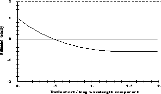
Now, if we calculate the estimated velocity on two different grids, with
spatial step  equal to one and two, as a function of the parameter,
R, we obtain the result illustrated in Figure 6.38.

Figure 6.38: Measured velocity for superposition of sinusoidal patterns as a
function of the ratio of short to long wavelength components. Dashed line:
 , continuous line:
  .
.
While on the coarser grid, the correct velocity is obtained (in this case);
on the finer one, the measured velocity depends on the value of R. In
particular, if R is greater than  , we obtain a velocity in the
opposite direction!
We propose a method for ``tuning'' the discretization grid to a measure of the reliability of the optical flow derived at a given scale. This measure is based on a local estimate of the errors due to noise and discretization, and is described in [Battiti:89g;91b].


