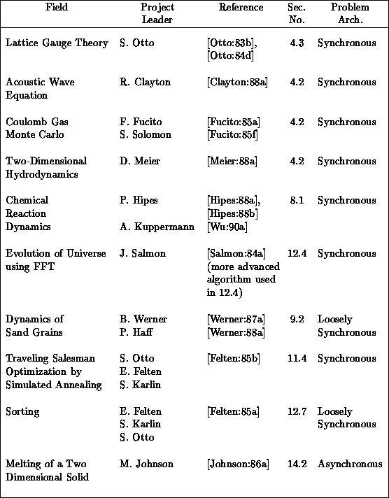
Table 4.2: The Ten Pioneer Hypercube Applications within C
 P
P


Table 4.2 indicates that 70 percent of our first set of applications were of the class we call synchronous. As remarked above, this could be expected in any such early work as these are the problems with the cleanest structure that are, in general, the simplest to code and, in particular, the simplest to parallelize. As already defined in Section 3.4, synchronous applications are characterized by a basic algorithm that consists of a set of operations which are applied identically in every point in a data set. The structure of the problem is typically very clear in such applications, and so the parallel implementation is easier than for the irregular loosely synchronous and asynchronous cases. Nevertheless, as we will see, there are many interesting issues in these problems and they include many very important applications. This is especially true for academic computations that address fundamental science. These are often formulated as studies of fundamental microscopic quantities such as the quark and gluon fundamental particles seen in QCD of Section 4.3. Fundamental microscopic entities naturally obey identical evolution laws and so lead to synchronous problem architectures. ``Real world problems''-perhaps most extremely represented by the battle simulations of Chapter 18 in this book-typically do not involve arrays of identical objects, but rather the irregular dynamics of several different entities. Thus, we will find more loosely synchronous and asynchronous problems as we turn from fundamental science to engineering and industrial or government applications. We will now discuss the structure of QCD in more detail to illustrate some general computational features of synchronous problems.

Table 4.2: The Ten Pioneer Hypercube Applications within C P
P
The applications using the Cosmic Cube were well established by 1984 and Table 4.2 lists the ten projects which were completed in the first year after we started our interdisciplinary project in the summer of 1983. All but one of these projects are more or less described in this book, while the other will be found in [Fox:88a]. They covered a reasonable range of application areas and formed the base on which we first started to believe that parallel computing works! Figure 4.3 illustrates the regular lattice used in QCD and its decomposition onto 64 nodes. QCD is a four-dimensional theory and all four dimensions can be decomposed. In our initial 64-node Cosmic Cube calculations, we used the three-dimensional decompositions shown in Figure 4.3 with the fourth dimension, as shown in Figure 4.4, and internal degrees of freedom stored sequentially in each node. Figure 4.3 also indicates one subtlety needed in the parallelization; namely, one needs a so-called red-black strategy with only half the lattice points updated in each of the two (``red'' and ``black'') phases. Synchronous applications are characterized by such a regular spatial domain as shown in Figure 4.3 and an identical update algorithm for each lattice point. The update makes use of a Monte Carlo procedure described in Section 4.3 and in more detail in Chapter 12 of [Fox:88a]. This procedure is not totally synchronous since the ``accept-reject'' mechanism used in the Monte Carlo procedure does not always terminate at the same step. This is no problem on an MIMD machine and even makes the problem ``slightly loosely synchronous.'' However, SIMD machines can also cope with this issue as all systems (DAP, CM-2, Maspar) have a feature that allows processors to either execute the common instruction or ignore it.
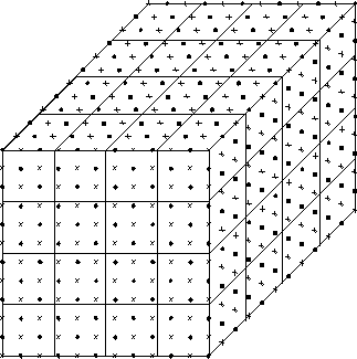
Figure 4.3: A  Problem Lattice Decomposed onto a 64-node Machine
Arranged as a
  Machine Lattice. Points labeled X (``red'') or
 (``black'') can be updated at the same time.
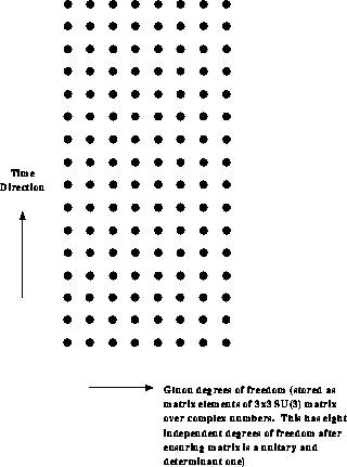
Figure: The 16 time and eight internal gluon degrees of freedom stored
at each point shown in Figure 4.3
Figure 4.5 illustrates the nearest neighbor algorithm used in QCD and very many problems described by local interactions. We see that some updates require communication and some don't. In the message-passing software model used in our hypercube work described in Chapter 5, the user is responsible for organizing this communication with an explicit subroutine call. Our later QCD calculations and the spin simulations of Section 4.4 use the data-parallel software model on SIMD machines where a compiler can generate their messaging. Chapter 13 will mention later projects which are aimed at producing a uniform data parallel Fortran or C compiler which will generate the correct message structure for either SIMD or MIMD machines on such regular problems as QCD.
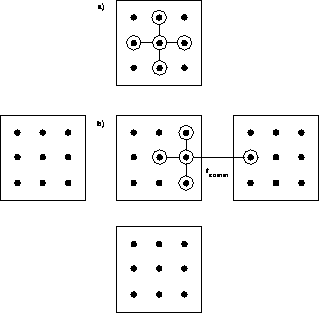
Figure 4.5: Template of a Local Update Involving No Communication in a) and
the Value to be Communicated in b).
The calculations in Sections 4.3 and 4.4 used a wide variety of machines, in-house and commercial multicomputers, as well as the SIMD DAP and CM-2. The spin calculations in Section 4.4 can have very simple degrees of freedom, including that of the binary ``spin'' of the Ising model. These are naturally suited to the single-bit arithmetic available on the AMT DAP and CM-2. Some of the latest Monte Carlo algorithms do not use the local algorithms of Figure 4.4 but exploit the irregular domain structure seen in materials near a critical point. These new algorithms are much more efficient but very much more difficult to parallelize-especially on SIMD machines. They are discussed in Section 12.8. We also see a taste of the ``embarrassingly parallel'' problem structure of Chapter 7 in Section 4.4. For the Potts simulation, we obtained parallelism not from the data domain (lattice of spins) but from different starting points for the evolution. This approach, described in more detail in Section 7.2, would not be practical for QCD with many degrees of freedom as one must have enough memory to store the full lattice in each node of the multicomputer.
Table 4.2 lists the early seismic simulations of the group
led by Clayton, whose C P work is reviewed in Section 18.1.
These solved the elastic wave equations using finite
difference methods as discussed in
Section 3.5. The equations are iterated with time steps
replacing the Monte Carlo iterations used above. This work is
described in Chapters 5 and 7 of [Fox:88a]
and represents methods that can tackle quite practical problems, for
example, predicting the response of complicated geological structures
such as the Los Angeles basin. The two-dimensional hydrodynamics work
of Meier [Meier:88a] is computationally similar, using the regular
decomposition and local update of Figures 4.3 and
4.5. These techniques are now very familiar and may seem
``old-hat.'' However, it is worth noting that, as described in
Chapter 13, we are only now in 1992 developing the
compiler technology that will automate these methods
developed ``by-hand'' by our early users. A much more sophisticated
follow-on to these early seismic wave simulations is the ISIS
interactive seismic imaging system described in Chapter 18.
Chapter 9 of [Fox:88a] explains the well-known synchronous
implementation of long-range particle dynamics. This algorithm was not used directly in any large C P
application as we implemented the much more efficient cluster
algorithms described in Sections 12.4, 12.5, and
12.8. The initial investigation of the vortex method of
Section 12.5 used the
  method [Harstad:87a]. We
also showed a parallel database used in Kolawa's thesis on how a
semi-analytic approach to QCD could be analyzed identically with the
long-range force problem
[Kolawa:86b;88a]. As explained in [Fox:88a],
one can use the long-range force algorithm in any case where the
calculation involves a set of N points with observables requiring
functions of every pair of which there are
  . In the language of
Chapter 3, this problem has a system dimension of one, whatever its geometrical dimension. This is
illustrated in Figures 4.6 and 4.7, which
represent
  in the form of Equations 3.10 and
3.13. We find
  for the
simple two-dimensional decompositions described for the Clayton and
Meier applications for Table 4.2. We increase range of
R ``interaction'' in Figure 4.7(a),(b)-defined
formally by

from small (nearest neighbor) R to  , the long-range force.
As shown in Figure 4.7(a),(b),
  decreases as R
increases with the limiting form
  independently of
  for
for  . Noederlinger
[Lorenz:87a] and Theiler [Theiler:87a;87b]
used such a ``long-range'' algorithm for
calculating the correlation dimension of a
chaotic dynamical system. This measures the essential number of
degrees of freedom for a complex system which in this case was a time
series becoming a plasma. The correction function
involved studying histograms of
  over the data points
  at time
  .
.
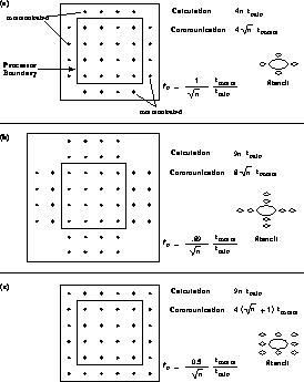
Figure 4.6: Some Examples of Communication Overhead as a Function of Increasing
Range of Interaction R.
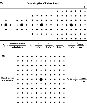
Figure 4.7: General Form of Communication Overhead for (a) Increasing and
(b) Infinite Range R
Fucito and Solomon [Fucito:85b;85f] studied a simple Coulomb gas which naturally had a long-range force. However, this was a Monte Carlo calculation that was implemented efficiently by an ingenious algorithm that cannot directly use the analysis of the particle dynamics (time-stepped) case shown in Figure 4.7. Monte Carlo is typically harder to parallelize than time evolution, where all ``particles'' can be evolved in time together. However, Monte Carlo updates can only proceed simultaneously if they involve disjoint particle sets. This implies the red-black ordering of Figure 4.5 and the requiring of a difficult asynchronous algorithm in the irregular melting problem of Section 14.2. Johnson's application was technically the hardest in our list of pioneers in Table 4.2.
Finally, Section 4.5 uses cellular automata ideas that lead to a synchronous architecture to grain dynamics, which, if implemented directly as in Section 9.2, would be naturally loosely synchronous. This illustrates that the problem architecture depends on the particular numerical approach.


