The usual error analysis of the SVD algorithms xGESVD and xGESDD in LAPACK (see subsection 2.3.4) or the routines in LINPACK and EISPACK is as follows [25,55]:
The SVD algorithm is backward stable. This means that the computed SVD,, is nearly the exact SVD of A+E where
, and p(m,n) is a modestly growing function of m and n. This means
is the true SVD, so that
and
are both orthogonal, where
, and
. Each computed singular value
differs from true
by at most
(we take p(m,n)=1 in the code fragment). Thus large singular values (those near) are computed to high relative accuracy and small ones may not be.
There are two questions to ask about the computed singular vectors: ``Are they orthogonal?'' and ``How much do they differ from the true eigenvectors?'' The answer to the first question is yes, the computed singular vectors are always nearly orthogonal to working precision, independent of how much they differ from the true singular vectors. In other words
for.
Here is the answer to the second question about singular vectors. The angular difference between the computed left singular vectorand a true ui satisfies the approximate bound
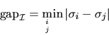
whereis the absolute gap between
must be redefined as
. The gaps may be easily computed from the array of computed singular values using function SDISNA. The gaps computed by SDISNA are ensured not to be so small as to cause overflow when used as divisors. The same bound applies to the computed right singular vector
and a true vector vi.
Letbe the space spanned by a collection of computed left singular vectors
, where
is a subset of the integers from 1 to n. Let
be the corresponding true space. Then
where
is the absolute gap between the singular values in4.1.
In the special case of bidiagonal matrices, the singular values and singular vectors may be computed much more accurately. A bidiagonal matrix B has nonzero entries only on the main diagonal and the diagonal immediately above it (or immediately below it). xGESVD computes the SVD of a general matrix by first reducing it to bidiagonal form B, and then calling xBDSQR (subsection 2.4.6) to compute the SVD of B. xGESDD is similar, but calls xBDSDC to compute the SVD of B. Reduction of a dense matrix to bidiagonal form B can introduce additional errors, so the following bounds for the bidiagonal case do not apply to the dense case.
Each computed singular value of a bidiagonal matrix is accurate to nearly full relative accuracy, no matter how tiny it is:
The following bounds apply only to xBDSQR. The computed left singular vector
whereis the relative gap between
In the very special case of 2-by-2 bidiagonal matrices, xBDSQR and xBDSDC call auxiliary routine xLASV2 to compute the SVD. xLASV2 will actually compute nearly correctly rounded singular vectors independent of the relative gap, but this requires accurate computer arithmetic: if leading digits cancel during floating-point subtraction, the resulting difference must be exact. On machines without guard digits one has the slightly weaker result that the algorithm is componentwise relatively backward stable, and therefore the accuracy of the singular vectors depends on the relative gap as described above.
Jacobi's method [34,99,91] is another algorithm for finding singular values and singular vectors of matrices. It is slower than the algorithms based on first bidiagonalizing the matrix, but is capable of computing more accurate answers in several important cases.