Let Ax=b be the system to be solved, and ![]() the computed
solution. Let n be the dimension of A.
An approximate error bound
for
the computed
solution. Let n be the dimension of A.
An approximate error bound
for ![]() may be obtained in one of the following two ways,
depending on whether the solution is computed by a simple driver or
an expert driver:
may be obtained in one of the following two ways,
depending on whether the solution is computed by a simple driver or
an expert driver:
      EPSMCH = SLAMCH( 'E' )
*     Get infinity-norm of A
      ANORM = SLANGE( 'I', N, N, A, LDA, WORK )
*     Solve system; The solution X overwrites B
      CALL SGESV( N, 1, A, LDA, IPIV, B, LDB, INFO )
      IF( INFO.GT.0 ) THEN
         PRINT *,'Singular Matrix'
      ELSE IF (N .GT. 0) THEN
*        Get reciprocal condition number RCOND of A
         CALL SGECON( 'I', N, A, LDA, ANORM, RCOND, WORK, IWORK, INFO )
         RCOND = MAX( RCOND, EPSMCH )
         ERRBD = EPSMCH / RCOND
      END IF
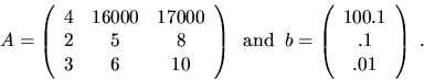
For example, suppose4.11
![]() ,
,
      CALL SGESVX( 'E', 'N', N, 1, A, LDA, AF, LDAF, IPIV,
     $             EQUED, R, C, B, LDB, X, LDX, RCOND, FERR, BERR,
     $             WORK, IWORK, INFO )
      IF( INFO.GT.0 ) PRINT *,'(Nearly) Singular Matrix'
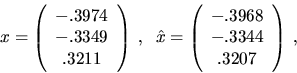
For the same A and b as above,
 ,
,
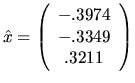
![]() ,
and the actual error is
,
and the actual error is
![]() .
.
This example illustrates that the expert driver provides an error bound with less programming effort than the simple driver, and also that it may produce a significantly more accurate answer.
Similar code fragments, with obvious adaptations, may be used with all the driver routines for linear equations listed in Table 2.2. For example, if a symmetric system is solved using the simple driver xSYSV, then xLANSY must be used to compute ANORM, and xSYCON must be used to compute RCOND.