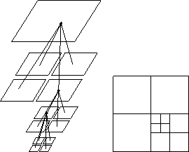
Figure 12.10: (a) Expanded and (b) Flat Representation of an Adaptive Tree


There are a number of ways to utilize this fact in a computer simulation [Appel:85a], [Barnes:86a], [Greengard:87b], [Zhao:87a]. The methods differ in choice of data structure, level of mathematical rigor, and complexity of the fundamental interactions. We shall consider an adaptive tree data structure, and an algorithm that treats each body independently. The algorithm begins by partitioning space into an oct-tree, that is, a tree whose nodes correspond to cubical regions of space. Each node may have up to eight daughter nodes, corresponding to the eight subcubes that are obtained by dividing in half in each Cartesian direction. The tree is defined by the following properties:

Figure 12.10: (a) Expanded and (b) Flat Representation of an Adaptive Tree

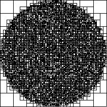
Figure 12.11: 10,000 Body Barnes-Hut Tree
The oct-tree provides a convenient data structure
which allows us to record the properties of the matter distribution on
all length scales. It is especially convenient for astrophysical
systems because it is adaptive. That is, the depth of the tree adjusts
itself automatically to the local particle density. In order to use an
approximation like Equation 12.5, we need to know certain
properties of the matter distribution in each cell. In the simplest
case, these properties are the mass and center-of-mass of the matter
distribution, but it is possible to use quadrupole moments
[Hernquist:87a], or higher-order moments [Salmon:90a] for
added accuracy. All of these properties may be computed by a bottom-up
traversal of the tree, combining the properties of the ``daughters'' of
a node to get the properties of the node itself. The time required for
this bottom-up traversal is proportional to the number of internal
nodes in the tree, that is,  .
.


