


``Local'' optimization is a method which has been used in compilers for many years and whose principles are well understood. We can see the evolutionary path to ``parallelizing compilers'' as follows.
The goal of automatic parallelization is obviously not new, just as parallel processors are not new. In the past, providing support for advanced technologies was in the realm of the compiler, which assumed the onus, for example, of hiding vectorizing hardware from the innocent users.
Performing these tasks typically involves a fairly simple line of thought shown by the ``flow diagram'' in Figure 13.12. Basically the simplest idea is to analyze the dependences between data objects within loops. If there are no dependences, then ``kick'' the vectorizer into performing all, or as many as it can handle, of the loop iterations at once. Classic vector code therefore has the appearance
DO 10 I=1,A(I) = B(I) + C(I)*D(I)
10 CONTINUE
DO 10 I=1,10000
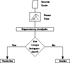
Figure 13.12: Vectorizability Analysis
We can easily derive parallelizing compilers from this type of technology by changing the box marked ``vectorize'' in Figure 13.12 to one marked ``parallelize.'' After all, if the loop iterations are independent, parallel operation is straightforward. Even better results can often be achieved by adding a set of ``restructuring operations'' to the analysis as shown in Figure 13.13.
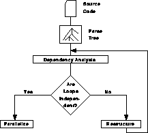
Figure 13.13: A Parallelizing Compiler
The idea here is to perform complex ``code transformations'' on cases which fail to be independent during the first dependence analysis in an attempt to find a version of the same algorithm with fewer dependences. This type of technique is similar to other compiler optimizations such as loop unrolling and code inlining [Zima:88a], [Whiteside:88a]. Its goal is to create new code which produces exactly the same result when executed but which allows for better optimization and, in this case, parallelization.
The emphasis of the two previous techniques is still on producing exactly the same result in both sequential and parallel codes. They also rely heavily on sophisticated compiler technology to reach their goals.
ASPAR takes a rather different approach. One of its first assumptions is that it may be okay for the sequential and parallel codes to give different answers!
In technical terms, this assumption removes the requirement that loop iterations be independent before parallelization can occur. In practical terms, we can best understand this issue by considering a simple example: image analysis.
One of the fundamental operations of image analysis is ``convolution.'' The basic idea is to take an image and replace each pixel value by an average of its neighbors. In the simplest case we end up with an algorithm that looks like
DO 20 J = 2,N-1
DO 20 J = A(I,J)=0.25*(A(I+1,J)+A(I-1,J)+A(I,J+1)+A(I,J-1))
20 CONTINUE
10 CONTINUE
DO 10 I = 2,N-1
To make this example complete, we show in Figure 13.14 the results of applying this operation to an extremely small (integer-valued) image.
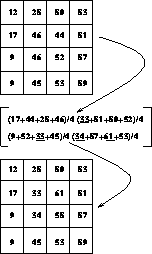
Figure 13.14: A Sequential Convolution
It is crucial to note that the results of this operation are not as trivial
as one might naively expect. Consider the value at the point (I=3, J=3)
which has the original value 52. To compute this value we are instructed to
add the values at locations A(2,2), A(2,4), A(3,2), and A(3,4).
If we looked only at the original data from the top of the figure, we might
then conclude that the correct answer is  .
.
Note that the source code, however, modifies the array A while
simultaneously using its values. As a result, the above calculation accesses
the correct array elements, but by the time we get around to computing the
value at  the values to the left and above have already been changed
by previous loop iterations. As a result the correct value at
the values to the left and above have already been changed
by previous loop iterations. As a result the correct value at  is
given by
is
given by  , where the
underlined values are those which have been calculated on previous loop
iterations.
, where the
underlined values are those which have been calculated on previous loop
iterations.
Obviously, this is no problem for a sequential program because the algorithm, as stated in the source code, is translated correctly to machine code by the compiler, which has no trouble executing the correct sequence of operations; the problems with this code arise, however, when we consider its parallelization.
The most obvious parallelization strategy is to simply partition the values to be updated among the available processors. Consider, for example, a version of this algorithm parallelized for four nodes.
Initially we divide up the original array A by assigning a quadrant
to each processor. This gives the situation shown in Figure 13.15.
If we divide up the loop iterations in the same way, we see that the process
updating the top-left corner of the array is to compute 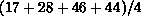 where the first two values are in its quadrant and the others lie to the
right and below the processor boundary. This is not too much of a
problem-on a shared-memory machine, we would
merely access the value ``44'' directly, while on a distributed-memory
machine, a message might be needed to transfer the value to our node.
In neither case is the procedure very complex; especially since we are
having the compiler or parallelizer do the actual communication for
us.
where the first two values are in its quadrant and the others lie to the
right and below the processor boundary. This is not too much of a
problem-on a shared-memory machine, we would
merely access the value ``44'' directly, while on a distributed-memory
machine, a message might be needed to transfer the value to our node.
In neither case is the procedure very complex; especially since we are
having the compiler or parallelizer do the actual communication for
us.
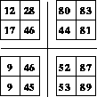
Figure 13.15: Data Distributed for Four Processors
The first problem comes in the processor responsible for the data in the
top-right quadrant. Here we have to compute 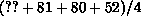 where the
values ``80'' and ``81'' are local and the value ``52'' is in another
processor's quadrant and therefore subject to the same issues just
described for the top-left processor.
where the
values ``80'' and ``81'' are local and the value ``52'' is in another
processor's quadrant and therefore subject to the same issues just
described for the top-left processor.
The crucial issue surrounds the value ``??'' in the previous expression. According to the sequential algorithm, this processor should wait for the top-left node to compute its value and then use this new result to compute the new data in the top-right quadrant. Of course, this represents a serialization of the worst kind, especially when a few moments' thought shows that this delay propagates through the other processors too! The end result is that no benefit is gained from parallelizing the algorithm.
Of course, this is not the way image analysis (or any of the other fields with similar underlying principles such as PDEs, Fluid mechanics, and so on) is done in parallel. The key fact which allows us to parallelize this type of code despite the dependences is the observation that: A large number of sequential algorithms contain data dependences that are not crucial to the correct ``physical'' results of the application.
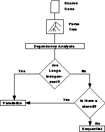
Figure 13.16: ASPAR's Decision Structure
In this case, the data dependence that appears to prevent parallelization is also present in the sequential code but is typically irrelevant. This is not to say that its effects are not present but merely that the large-scale behavior of our application is unchanged by ignoring it. In this case, therefore, we allow the processor with the top-right quadrant of the image to use the ``old'' value of the cells to its left while computing new values, even though the processor with the top-left quadrant is actively engaged in updating them at the very same time that we are using them!
While this discussion has centered on a particular type of application and the intricacies of parallelizing it, the arguments and features are common to an enormous range of applications. For this reason ASPAR works from a very different point of view than ``parallelizing'' compilers: its most important role is to find data dependences of the form just described-and break them! In doing this, we apply methods that are often described as stencil techniques.
In this approach, we try to identify a relationship between a new data value and the old values which it uses during computation. This method is much more general than simple dependence analysis and leads to a correspondingly higher success rate in parallelizing programs. The basic flow of ASPAR's deliberations might therefore be summarized in Figure 13.16.
It is important to note that ASPAR provides options to enforce strict dependence checking as well as to override ``stencil-like'' dependences. By adopting this philosophy of checking for simple types of dependences, ASPAR more nearly duplicates the way humans address the issue of parallelization and this leads to its greater success. The use of advanced compilation techniques could also be useful, however, and there is no reason why ASPAR should ``give up'' at the point labelled ``Sequential'' in Figure 13.16. A similar ``loopback'' via code restructuring, as shown in Figure 13.13, would also be possible in this scenario and would probably yield good results.