Computing Interior Eigenvalues

For restart purposes, specially if one is heading for interior eigenvalues, the harmonic Ritz vectors have been advocated for symmetric matrices [331]; see also §4.7.4.

The concept of harmonic Ritz values [349] is easily generalized for unsymmetric matrices [411]. As we have seen, the Jacobi-Davidson methods generate basis vectors ${v}_1, \ldots, {v}_{m}$ for a subspace ${\cal V}_{m}$. For the projection of $A$ onto this subspace we have to compute the vectors ${w}_j\equiv A{v}_j$. The inverses of the Ritz values of $A^{-1}$, with respect to the subspace spanned by the ${w}_j$, are called the harmonic Ritz values. The harmonic Ritz values can be computed without inverting $A$, since a harmonic Ritz pair $(\widetilde{\theta}_j^{({m})},\widetilde{u}_j^{({m})})$ satisfies

$$A\widetilde{u}_j^{({m})} - \widetilde\theta_j^{({m})}\widet... ...perp {\cal W}_{m}\equiv \mbox{span}\{{w}_1,\ldots , {w}_{m}\}$$ (209)

for $\widetilde{u}_j^{({m})} \in {V}_{m}$ and $\widetilde{u}_j^{({m})}\neq 0$. This implies that the harmonic Ritz values are the eigenvalues of the pencil $(W_{m}^\ast AV_{m}, W_{m}^\ast V_{m})$:

$$W_{m}^\ast AV_{m} s_j^{({m})} - \widetilde\theta_j^{({m})} W_{m}^\ast V_{m} s_j^{({m})} =0 .$$

The exterior standard Ritz values usually converge to exterior eigenvalues of $A$. Likewise, the interior harmonic Ritz values for the shifted matrix $A-\tau I$ usually converge towards eigenvalues $\lambda\neq \tau$ closest to the shift $\tau$. Fortunately, the search subspaces ${\cal V}_{m}$ for the shifted matrix and the unshifted matrix coincide, which facilitates the computation of harmonic Ritz pairs. For reasons of stability we construct both ${V}_{m}$ and ${W}_{m}$ to orthonormal: ${W}_{m}$ is such that $(A-\tau I){V}_{m}={W}_{m} M^A_{m}$, where $M^A_{m}$ is ${m}$ by ${m}$ upper triangular.

In the resulting scheme we compute a (partial) Schur decomposition rather than a partial eigendecomposition. That is, we wish to compute vectors ${q}_1,\ldots, {q}_{k}$, such that $A{Q}_k={Q}_k{R}_k$, with ${Q}_{k}^\ast {Q}_{k}=I_{k}$, and ${R}_{k}$ is a ${k}$ by ${k}$ upper triangular matrix. The diagonal elements of ${R}_{k}$ represent eigenvalues of $A$, and the corresponding eigenvectors of $A$ can be computed from ${Q}_{k}$ and ${R}_{k}$.

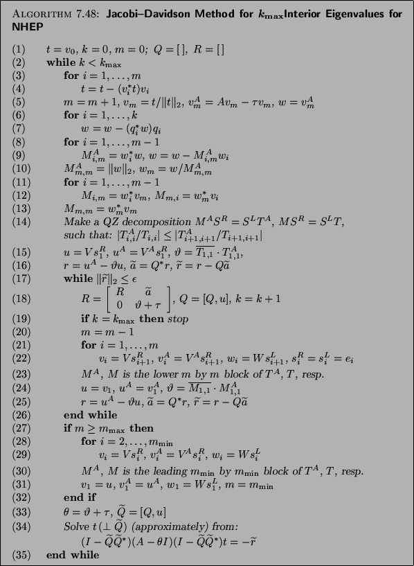
An algorithm for Jacobi-Davidson, with partial reduction to Schur form and based on harmonic Ritz values and vectors, is given in Algorithm 7.19. The algorithm includes restart and deflation techniques. It can be used for the computation of a number of eigenvalues close to $\tau$.

To apply this algorithm we need to specify a starting vector ${v}_0$, a tolerance $\epsilon$, a target value $\tau$, and a number ${k}_{\max}$ that specifies how many eigenpairs near $\tau$ should be computed. The value of ${m}_{\max}$ denotes the maximum dimension of the search subspace. If it is exceeded, then a restart takes place with a subspace of specified dimension ${m}_{\min}$.

On completion the $k_{\max}$ eigenvalues close to $\tau$ are delivered, and the corresponding reduced Schur form $AQ=QR$, where $Q$ is $n$ by $k_{\max}$ orthogonal and $R$ is $k_{\max}$ by $k_{\max}$ upper triangular. The eigenvalues are on the diagonal of $R$. The computed Schur form satisfies $\Vert A q_{j}- {Q} R e_{j}\Vert _2\leq j \epsilon$, where $q_j$ is the $j$th column of $Q$.

We will comment on some parts of the algorithm in view of our discussions in previous subsections.

(1)

Initialization phase.

(3)-(4)

The newly computed correction is made orthogonal with respect to the current search subspace by means of modified Gram-Schmidt. We have chosen to store also the matrix $V^A\equiv A{V}-\tau {V}$; ${v}_{m}^A$ is the expansion vector for this matrix. The expansion vector for ${W}$ is obtained by making ${v}_{m}^A$ orthogonal with respect to the space of detected Schur vectors and with respect to the current test subspace by means of modified Gram-Schmidt. The Gram-Schmidt steps can be replaced, for improved numerical stability, by the template given in Algorithm 4.14.

${V}$ denotes the $n$ by ${m}$ matrix with columns ${v}_j$; likewise $W$ and $V^A$.

(8)-(9)

The values ${M}_{i,j}$ represent elements of the square ${m}$ by ${m}$ matrix ${M}\equiv {W}^\ast {V}$. The values $M^A_{i,j}$ represent elements of the ${m}$ by ${m}$ upper triangular ${M^A}\equiv W^\ast V^A$.

(Note that $V^A={W} {M^A}+{Q}{F}$, if ${F}\equiv{Q}^\ast V^A$. Therefore, $V^A$ can be reconstructed from ${W}$, ${M^A}$, ${Q}$, and ${F}$. In particular, $r$ can be computed from these quantities. Instead of storing the ${n}$-dimensional matrix $V^A$, it suffices to store the ${k}$ by ${m}$ matrix ${F}$ (of elements ${q}_i^\ast {w}$, computed in (3)-(4)). This approach saves memory space. However, for avoiding instabilities, the deflation procedure needs special attention.)

(14)

At this point the QZ decomposition (generalized Schur form) of the matrix pencil $({M^A},{M})$ has to be be computed: ${M^A} {S}^R={S}^L{T^A}$ and ${M}{S}^R={S}^L {T}$, where ${S}^R$ and ${S}^L$ are unitary and ${T^A}$ and ${T}$ are upper triangular. This can be done with a suitable routine for dense matrix pencils from LAPACK.

In each step, the Schur form has to be sorted such that $\vert T^A_{1,1}/{T}_{1,1}\vert$ is smallest. Only if ${m}\geq {m}_{\max}$ does the sorting of the Schur form have to be such that all of the ${m}_{\max}$ leading diagonal elements of ${T^A}$ and ${T}$ represent the ${m}_{\max}$ harmonic Ritz values closest to $0$. For ease of presentation we sorted all diagonal elements here.

For an algorithm of the sorting of a generalized Schur form, see [33,448,449] and [171, Chap. 6B].

The matrix ${S^R}$ is $m$ by $m$ with columns ${s}_j^R$; likewise ${S^L}$.

(15)

The value of $\theta$ needs some attention. We have chosen to compute the Rayleigh quotient $\vartheta$ (instead of the harmonic Ritz value) corresponding to the harmonic Ritz vector ${u}$ (see [412]). The Rayleigh quotient follows from the requirement that $(A-\tau I){u}-\vartheta {u}\perp {u}$ instead of $\perp {W}$; then $r\perp {u}$. $\overline{{T}_{1,1}}$ denotes the complex conjugate of ${{T}_{1,1}}$.

(17)

The stopping criterion is to accept a Schur vector approximation as soon as the norm of the residual (for the normalized Schur vector approximation) is below $\epsilon$. This means that we accept inaccuracies in the order of $\epsilon$ in the computed eigenvalues, and inaccuracies (in angle) in the eigenvectors of $O(\epsilon)$ (provided that the concerned eigenvalue is simple and well separated from the others and the left and right eigenvectors have a small angle).

Detection of all wanted eigenvalues cannot be guaranteed; see note (13) for Algorithm 4.17 (p. ).

(20)

This is a restart after acceptance of an approximate eigenpair.

(27)

At this point we have a restart when the dimension of the subspace exceeds ${m}_{\max}$. After a restart the Jacobi-Davidson iterations are resumed with a subspace of dimension ${m}_{\min}$.

(33)

The deflation with computed eigenvectors is represented by the factors with ${Q}$. The matrix ${Q}$ has the converged eigenvectors as its columns. If a left preconditioner ${K}$ is available for the operator $A-\theta I$, then with a Krylov solver similar reductions are realizable as in the situation for exterior eigenvalues. A template for the efficient handling of the left-preconditioned operator is given in Algorithm 4.18.