Basic Algorithm

The basic form of the Jacobi-Davidson algorithm is given in Algorithm 4.13. Later, we will describe more sophisticated variants with restart and other strategies.

In each iteration of this algorithm an approximated eigenpair $(\theta,{u})$ for the eigenpair of the Hermitian matrix $A$, corresponding to the largest eigenvalue of $A$, is computed. The iteration process is terminated as soon as the norm of the residual $A{u}-\theta {u}$ is below a given threshold $\epsilon$.

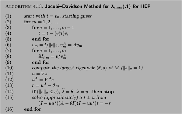
To apply this algorithm we need to specify a starting vector ${v}_0$ and a tolerance $\epsilon$. On completion an approximation for the largest eigenvalue $\lambda=\lambda_{\max}(A)$ and its corresponding eigenvector ${x}={x}_{\max}$ is delivered. The computed eigenpair $(\widetilde\lambda, \widetilde{x})$ satisfies $\Vert A\widetilde{x} - \widetilde\lambda\widetilde{x} \Vert\leq \epsilon$.

We will now describe some implementation details, referring to the respective phases in Algorithm 4.13.

(1)

This is the initialization phase of the process. The search subspace is expanded in each iteration by a vector ${t}$, and we start this process with a given vector $t=v_0$. Ideally, this vector should have a significant component in the direction of the wanted eigenvector. Unless one has some idea of the wanted eigenvector, it may be a good idea to start with a random vector. This gives some confidence that the wanted eigenvector has a nonzero component in the starting vector, which is necessary for detection of the eigenvector.

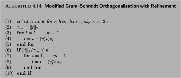
(3)-(5)

This represents the modified Gram-Schmidt process for the orthogonalization of the new vector $t$ with respect to the set ${v}_1, \ldots, {v}_{{m}-1}$. If ${m}=1$, this is an empty loop. Let ${t}_{in}$ represent the vector before the start of the orthogonalization, and ${t}_{out}$ the vector that results at completion of phase (3)-(5). It is advisable (see [96]) to repeat the Gram-Schmidt process one time if $\Vert{t}_{out}\Vert _2/\Vert{t}_{in}\Vert _2\leq \kappa$, where $\kappa$ is a modest constant, say $\kappa=.25$. This guarantees that the loss of orthogonality is restricted to $1/\kappa$ times machine precision, in a relative sense. The template for this modified Gram-Schmidt orthogonalization with iterative refinement is given in Algorithm 4.14.

(7)-(9)

In this phase, computation of the ${m}$th column of the upper triangular part of the matrix ${M}\equiv {V}^\ast A{V}$ occurs. The matrix ${V}$ denotes the $n$ by ${m}$ matrix with columns ${v}_j$, ${V^A}$ likewise.

(10)

Computing the largest eigenpair of the ${m}\times {m}$ Hermitian matrix ${M}$, with elements ${M}_{i,j}$ in its upper triangular part, can be done with the appropriate routines from LAPACK (see §4.2).

(12)

The vector ${u^A}$ may either be updated as described here or recomputed as ${u^A}=A{u}$, depending on which is cheapest. The choice is between an ${m}$-fold update and another multiplication with $A$; if $A$ has fewer than $m$ nonzero elements on average per row, the computation via $A{u}$ is preferable. If ${u^A}$ is computed as $A{u}$, it is not necessary to store the vectors $v^A_j$.

(14)

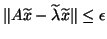
The algorithm is terminated if $\Vert A{u}-\theta {u}\Vert _2\leq \epsilon$. In that case $A$ has an eigenvalue $\lambda$ for which $\vert\lambda - \theta\vert\leq \epsilon$. For the corresponding normalized eigenvector there is a similar bound on the angle, provided that $\lambda$ is simple and well separated from the other eigenvalues of $A$. That case leads also to a sharper bound for $\lambda$; see (4.5) or §4.8.

Convergence to a $\lambda\neq\lambda_{\max}(A)$ may take place, but is in general unlikely. It happens, for instance, if $v_0\perp {x}_{\max}$, or if the selected $\theta$ is very close to an eigenvalue $\lambda\neq\lambda_{\max}(A)$. This may happen for any iterative solver, in particular if $\epsilon$ is taken not small enough (say, larger than the square root of machine precision).

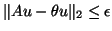
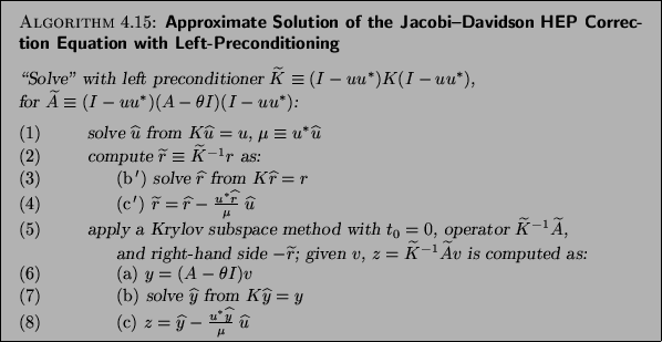
(15)

The approximate solution for the expansion vector ${t}$ can be computed with a Krylov solver, for instance, MINRES, or with SYMMLQ. With left- or right-preconditioning one has to select a Krylov solver for unsymmetric systems (like GMRES, CGS, or Bi-CGSTAB), since the preconditioned operator is in general not symmetric. A template for the approximate solution, with a left-preconditioned Krylov subspace method of choice, is given in Algorithm 4.15. 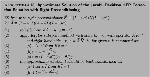The right preconditioned case, which is slightly more expensive, is covered by the template in Algorithm 4.16. For iterative Krylov subspace solvers see [41]. The approximate solution has to be orthogonal to ${u}$, but that is automatically the case with Krylov solvers if one starts with an initial guess orthogonal to ${u}$, for instance, ${t}_0=0$. In most cases it is not necessary to solve the correction equation to high precision; a relative precision of $2^{-m}$ in the ${m}$th iteration seems to suffice. It is advisable to put a limit to the number of iteration steps for the iterative solver.

Davidson [99] suggested taking ${t}=(\mbox{\rm diag}(A)-\theta I)^{-1}r$, but in this case ${t}$ is not orthogonal with respect to ${u}$. Moreover, for diagonal matrices this choice leads to stagnation, which is an illustration of the problems in this approach.

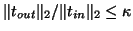
In order to restrict storage, the algorithm can be terminated at some appropriate value ${m}={m}_{\max}$ and restarted with $v_0$ as the latest value of ${u}$. We will describe a variant of the Jacobi-Davidson algorithm with a more sophisticated restart strategy in §4.7.3.

Note that most of the computationally intensive operations, i.e., those operations the cost of which is proportional to $n$, can easily be parallelized. Also, the multiple vector updates can be performed by the appropriate Level 2 BLAS routines (see §10.2).

In the coming subsections we will describe more sophisticated variants of the Jacobi-Davidson algorithm. In §4.7.3 we will introduce a variant that allows for restarts, which is convenient if one wants to keep the dimensions of the involved subspaces limited. This variant is also suitable for a restart after an eigenpair has been discovered, in order to locate the next eigenpair. The technique is based on deflation. The resulting algorithm is designed for the computation of a few of the largest or smallest eigenvalues of a given matrix.

In §4.7.4 we will describe a variant of the Jacobi-Davidson method that is suitable for the computation of interior eigenvalues of $A$.