Algorithm

The non-Hermitian Lanczos method as presented in Algorithm 7.13 below is a two-sided iterative algorithm with starting vectors $p_1$ and $q_1$. It can be viewed as biorthogonalizing, via a two-sided Gram-Schmidt procedure, the two Krylov sequences

$$\{ q_1,Aq_1,A^2q_1,\ldots \} \quad \mbox{and} \quad \{ p_1, A^{\ast}p_1, (A^{\ast})^2 p_1, \ldots\}.$$

The two sequences of vectors $\{q_i\}$ and $\{p_i\}$ are generated using the three-term recurrences:

$$\beta_{j+1} q_{j+1} = Aq_j - \alpha_j q_j - \gamma_j q_{j-1},$$ (139)

$$\bar{\gamma}_{j+1} p_{j+1} = A^{\ast} p_j - \bar{\alpha}_j p_j - \bar{\beta}_j p_{j-1}.$$ (140)

The vectors $\{q_i\}$ and $\{p_i\}$ are called Lanczos vectors, span ${\cal K}^j(A,q_1)$ and ${\cal K}^j(A^{\ast},p_1)$, respectively, and are biorthogonal, namely, $p^{\ast}_{k} q_{\ell} = 0$ if $k \neq \ell$ and $w^{\ast}_{k} v_{k} = 1$. In matrix notation, at the $j$th step, the Lanczos method generates two $n \times j$ matrices $Q_j$ and $P_j$:

$$Q_j = [ q_1, q_2, \ldots, q_j ], \quad \quad P_j = [ p_1, p_2, \ldots, p_j ]$$

and

$$T_j=\left[ \begin{array}{ccccc} \alpha_1 & \gamma_2 &&&\\ \... ...ts&\gamma_{j}\\ &&&\beta_{j}&\alpha_j\\ \end{array} \right].$$

The computed quantities satisfy the governing relations, called Lanczos factorizations:

$$AQ_j = Q_j T_j + \beta_{j+1} q_{j+1} e_{j}^{\ast}\;,$$ (141)

$$A^{\ast} P_j = P_{j}T_{j}^{\ast} + \bar{\gamma}_{j+1} p_{j+1} e_j^{\ast} \;,$$ (142)

$$P_j^{\ast} Q_j = I_j\;.$$ (143)

In addition, $P^{\ast}_j q_{j+1} = 0$ and $p^{\ast}_{j+1} Q_{j} = 0$. The relation (7.37) shows that the Lanczos vectors (bases) are biorthonormal. But note that neither $Q_j$ nor $P_j$ is unitary. In the Lanczos bases, the matrix $A$ is represented by a non-Hermitian tridiagonal matrix,

$$P_j^{\ast} AQ_j = T_j.$$ (144)

At any step $j$, we may compute eigensolutions of $T_j$,

$$T_j z_i^{(j)} = \theta_i^{(j)} z_i^{(j)} \quad \mbox{and} \quad (w_i^{(j)})^{\ast} T_j = \theta_i^{(j)} (w_i^{(j)})^{\ast}\;.$$

Eigenvalues of $A$ are approximated by the eigenvalues $\theta_i^{(j)}$ of $T_j$, which are called Ritz values.

To each Ritz value $\theta_i^{(j)}$ there correspond right and left Ritz vectors,

$$x_i^{(j)}=Q_jz_i^{(j)} \quad \mbox{and} \quad y_i^{(j)}=P_jw_i^{(j)}\;.$$ (145)

The convergence of the Ritz values and vectors to eigenvalues and eigenvectors of the original matrix $A$ can be evaluated by comparing the norms of the residuals

$$r_i^{(j)} = Ax_i^{(j)} - \theta_i^{(j)} x_i^{(j)},$$ (146)

$$(s_i^{(j)})^{\ast} = (y_i^{(j)})^{\ast} A - \theta_i^{(j)} (y_i^{(j)})^{\ast}$$ (147)

to the norms of $x_i^{(j)}$ and $y_i^{(j)}$, respectively. Moreover, by equation (7.35), the right residual vector becomes

$$r_i^{(j)} = \beta_{j+1} q_{j+1} (e^{\ast}_j z_i^{(j)})\;,$$ (148)

and by equation (7.36), the left residual vector becomes

$$(s_i^{(j)})^{\ast} = \gamma_{j+1} p^{\ast}_{j+1} ((w_i^{(j)})^{\ast} e_j)\;.$$ (149)

Therefore, as in the Hermitian case (see §4.4), the residual norms are available without explicitly computing the Ritz vectors $x^{(j)}_i$ and $y^{(j)}_i$, though $\Vert x_i^{(j)} \Vert _2$ and $\Vert y_i^{(j)} \Vert _2$ are unavailable. See §7.8.2 for a more detailed discussion of this topic.

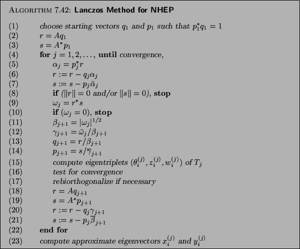
We will now comment on certain steps of Algorithm 7.13:

(1)

The initial starting vectors $p_1$ and $q_1$ are best selected by the user to embody any available knowledge concerning $A$'s wanted eigenvectors. In the absence of such knowledge, one can choose $q_1$ with randomly distributed entries and let $p_1 = q_1$.

(2), (3), (18), (19)

The matrix-vector multiplication routines to multiply $A$ and $A^{\ast}$ by an arbitrary vector are required in these steps. This is usually the computational bottleneck. See the discussion of convergence properties below for implementation notes in the shift-and-invert case.

(8)

This is one of two cases in which the method may break down. In fact, this is a desirable breakdown. If $r$ is null, then the Lanczos vectors $\{q_1,q_2,\ldots,q_j\}$ span a (right) invariant subspace of $A$; each Ritz value and corresponding right Ritz vector is an exact eigenvalue and eigenvector of $A$. The Lanczos algorithm may be continued if necessary by taking as $q_{j+1}$ any vector such that $P_{j}^{*} q_{j+1} = 0$ and setting $\beta_{j+1} =0$. Similar actions can be taken when $s$ or both $r$ and $s$ vanish.

In practice, an exact null vector is rare. It does happen that the norms of $r$ and/or $s$ are tiny. A tolerance value to detect a tiny $\Vert r\Vert _2$ compared to $\Vert Q\Vert _2\Vert T\Vert _2$ or a tiny $\Vert s\Vert _2$ compared to $\Vert P\Vert _2\Vert T\Vert _2$ should be given. A default tolerance value is a small multiple of $\epsilon$, the machine precision.

(10)

If $\omega_j = r^{\ast} s=0$ before either $r$ or $s$ vanishes, the method has an essential breakdown. In most cases we may continue finding new vectors in the Krylov subspaces ${\cal K}^{j+k}(A,r)$ and ${\cal K}^{j+k}(A^{\ast},s)$ for some integer $k > 0$, and add a block outside the three diagonals of $T_j$; this so-called look-ahead procedure is described in [178] and implemented in QMRPACK (see §7.8.3 below). If, however, our starting vectors $q_1$ and $p_1$ have different minimal polynomials (or, say, $p_1$ and $q_1$ are composites of different set of eigenvectors), even this does not help, and we have a mismatch, also called incurable breakdown. See [354] for a further discussion. A different treatment of the breakdown is discussed in §7.9.

In practice, exact breakdown is rare. Near breakdowns occur more often; i.e., $\omega_j$ is nonzero but extremely small in absolute value. Near breakdowns cause stagnation and instability. Any criterion for detecting a near breakdown either must stop too early in some situations or stops too late in other cases. A reasonable compromise criterion for detecting near breakdowns in an eigenvalue problem is to stop if $\vert\omega_j\vert \leq \sqrt{\epsilon} \Vert r\Vert _2 \Vert s\Vert _2$.

(15)

The cost of computing eigendecomposition of the tridiagonal matrix $T_j$ by the QR algorithm (see §7.3) is approximately $30j^3$ floating point operations per iteration, and the cumulative cost for steps 1 to $j$ is $15 j^4$ floating point operations. Solving the eigenproblem periodically, say at every 10 steps, reduces this cost.

No stable algorithm has been found for an eigenvalue problem that approximates the eigenvalues of a general tridiagonal in $j^2$ floating point operations, though recently conditionally stable algorithms such as [94,189] have been proposed. No software implementation of the Lanczos algorithm known to the authors employs a fast conditionally stable eigensolver.

(16)

Computation halts once bases $Q_j$ and $P_j$ have been determined so that eigenvalues $\theta_i^{(j)}$ of $T_j$ (7.38) approximate all the desired eigenvalues of $A$ with sufficiently small residuals, which are calculated according to the equations (7.42) and (7.43). Convergence properties are discussed in more detail in §7.8.2.

If there is no re-biorthogonalization (see [105]), then in finite precision arithmetic after a Ritz value converges to an eigenvalue of $A$, copies of this Ritz value will appear at later Lanczos steps. For example, a cluster of Ritz values of the reduced tridiagonal matrix, $T_j$, may approximate a single eigenvalue of the original matrix $A$. A spurious value [93] is a simple Ritz value that is also an eigenvalue of the matrix of order $j-1$ obtained by deleting the first row and column from $T_j$. Such spurious values should be discarded from consideration. Eigenvalues of $T_j$ which are not spurious are identified as approximations to eigenvalues of the original matrix $A$ and are tested for convergence.

(17)

As in the Hermitian case, in the presence of finite precision arithmetic, the biorthogonality of computed Lanczos vectors $\{q_i\}$ and $\{p_i\}$ deteriorates. One may use the two-sided modified Gram-Schmidt (TSMGS) process [354] to re-biorthogonalize the $(j+1)$st Lanczos vectors;

 		 		 for $i=1,2,\ldots,j$ 

$q_{j+1} = q_{j+1} - q_i (p^{\ast}_i q_{j+1})$ 

$p_{j+1} = p_{j+1} - p_i (q^{\ast}_i p_{j+1})$ 


end for

Applying the TSMGS process at each step is very costly and becomes a computational bottleneck. In [105], an efficient alternative scheme is proposed. This topic is revisited in §7.9.