The fundamental data object in the LU factorization algorithm presented in Section 4.1 is a block-partitioned matrix. In this section, we describe the block-cyclic method for distributing such a matrix over a two-dimensional mesh of processes, or template. In general, each process has an independent thread of control, and with each process is associated some local memory directly accessible only by that process. The assignment of these processes to physical processors is a machine-dependent optimization issue, and will be considered later in Section 7.
An important property of the class of data distribution we shall use is that
independent decompositions are applied over rows and columns. We shall,
therefore, begin by considering the distribution of a vector of M data objects
over P processes. This can be described by a mapping of the
global index, m, of a data object to an index pair (p,i), where p
specifies the process to which the data object is assigned, and i specifies
the location in the local memory of p at which it is stored. We shall
assume ![]() and
and ![]() .
.
Two common decompositions are the block and the cyclic
decompositions
[48, 30].
The block decomposition, which is often used when the computational load is
distributed homogeneously over a regular
data structure such as a Cartesian grid, assigns contiguous entries in the
global vector to the processes in blocks.
![]()
where ![]() , and
, and ![]() denotes the greatest
integer less than or equal to x. The cyclic decomposition (also known as the
wrapped or scattered decomposition) is commonly used to improve load balance
when the computational load is distributed inhomogeneously over a
regular data structure. The cyclic decomposition
assigns consecutive entries in the global vector to successive different
processes,
denotes the greatest
integer less than or equal to x. The cyclic decomposition (also known as the
wrapped or scattered decomposition) is commonly used to improve load balance
when the computational load is distributed inhomogeneously over a
regular data structure. The cyclic decomposition
assigns consecutive entries in the global vector to successive different
processes,
![]()
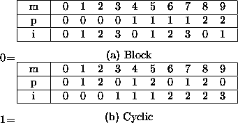
Examples of the block and cyclic decompositions are shown in
Figure 8.

Figure 8: Examples of block and cyclic decompositions of
M=10 data objects over P=3 processes.The global index m is mapped
to the process number, p, and local index, i.
The block cyclic decomposition is a generalization of the block and cyclic
decompositions in which blocks
of consecutive data objects are distributed cyclically over the processes.
In the block cyclic decomposition the mapping of the global index, m, can
be expressed as ![]() , where p is the process
number, b is the block number in process p, and i is the index
within block b to which m is mapped. Thus, if the number of
data objects in a block is r, the block cyclic
decomposition may be written,
, where p is the process
number, b is the block number in process p, and i is the index
within block b to which m is mapped. Thus, if the number of
data objects in a block is r, the block cyclic
decomposition may be written,
![]()
where T=rP.
It should be noted that this reverts to the cyclic decomposition when
r=1, with local index i=0 for all blocks. A block decomposition is
recovered when r=L, in which case there is a single block in
each process with block number b=0.
The inverse mapping of the triplet (p,b,i) to a global index is given by,
![]()
where B=p+bP is the global block number.
The block cyclic decomposition is one of the data distributions supported
by High Performance Fortran (HPF)
[38], and has been previously used, in one form or another, by several
researchers (see
[1, 4, 5, 9, 22, 26, 44, 46, 47]
for examples of its use).
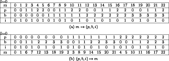
The block cyclic decomposition is illustrated with an example in
Figure 9.

Figure 9: An example of the block cyclic decomposition of M=23 data objects
over P=3 processes for a block size of r=2. (a) shows the mapping from
global index, m, to the triplet (p,b,i), and (b) shows the inverse
mapping.
The form of the block cyclic decomposition given by Eq. 9 ensures
that the block with global index 0 is placed in process 0, the next
block is placed in process 1, and so on. However,
it is sometimes necessary to offset the processes relative to the global block
index so that, in general, the first block is placed in process ![]() , the
next in process
, the
next in process ![]() , and so on. We, therefore, generalize the
block cyclic decomposition by replacing m on the righthand
side of Eq. 9 by
, and so on. We, therefore, generalize the
block cyclic decomposition by replacing m on the righthand
side of Eq. 9 by ![]() to give,
to give,

Equation 10 may also be generalized to,
![]()
where now the global block number is given by ![]() .
It should be noted that in processes with
.
It should be noted that in processes with ![]() , block 0 is not within the
range of the block cyclic mapping and it is, therefore, an error to
reference it in any way.
, block 0 is not within the
range of the block cyclic mapping and it is, therefore, an error to
reference it in any way.
In decomposing an ![]() matrix we apply independent block cyclic
decompositions in the row and column directions. Thus, suppose
the matrix rows are distributed with block size r and offset
matrix we apply independent block cyclic
decompositions in the row and column directions. Thus, suppose
the matrix rows are distributed with block size r and offset ![]() over P processes by the block cyclic mapping
over P processes by the block cyclic mapping ![]() ,
and the matrix columns are distributed with block size s and
offset
,
and the matrix columns are distributed with block size s and
offset ![]() over Q
processes by the block cyclic mapping
over Q
processes by the block cyclic mapping ![]() . Then the matrix element
indexed globally by (m,n) is mapped as follows,
. Then the matrix element
indexed globally by (m,n) is mapped as follows,

The decomposition of the matrix can be regarded as the tensor
product of the row and column decompositions, and we can write,
![]()
The block cyclic matrix decomposition given by Eqs. 13 and
14
distributes blocks of size ![]() to a mesh of
to a mesh of ![]() processes.
We shall refer to this mesh as the process template, and
refer to processes by their position in the template. Equation 14
says that global index (m,n) is mapped to process (p,q), where it
is stored in the block at location (b,d) in a two-dimensional array of blocks.
Within this block it is stored at location (i,j).
The decomposition is completely specified by the parameters r, s,
processes.
We shall refer to this mesh as the process template, and
refer to processes by their position in the template. Equation 14
says that global index (m,n) is mapped to process (p,q), where it
is stored in the block at location (b,d) in a two-dimensional array of blocks.
Within this block it is stored at location (i,j).
The decomposition is completely specified by the parameters r, s, ![]() ,
,
![]() , P, and Q.
In Figure 10 an example is given of the block cyclic decomposition
of a
, P, and Q.
In Figure 10 an example is given of the block cyclic decomposition
of a ![]() matrix for block size
matrix for block size ![]() , a process template
, a process template
![]() , and a template offset
, and a template offset ![]() . Figure
11 shows the
same example but for a template offset of (1,2).
. Figure
11 shows the
same example but for a template offset of (1,2).
The block cyclic decomposition can reproduce most of the data distributions
commonly used in linear algebra computations on parallel computers. For
example, if Q=1 and ![]() the block row decomposition is
obtained. Similarly, P=1 and
the block row decomposition is
obtained. Similarly, P=1 and ![]() gives a block column
decomposition. These decompositions, together with row and column cyclic
decompositions, are shown in Figure 12. Other commonly used
block cyclic matrix decompositions are shown in Figure 13.
gives a block column
decomposition. These decompositions, together with row and column cyclic
decompositions, are shown in Figure 12. Other commonly used
block cyclic matrix decompositions are shown in Figure 13.