Next: Refined Projection Methods.
Up: Basic Ideas Y. Saad
Previous: Oblique Projection Methods.
Contents
Index
Harmonic Ritz Values.
Our introduction of the Ritz values, in relation with Krylov subspaces,
suggests that they tend to approximate exterior eigenvalues better than
interior ones. This is supported by theory as well as borne out by
experience. Ritz values that are located in the interior part of the
spectrum can usually be considered as bad approximations for some exterior
eigenvalues, and the corresponding Ritz vectors often have a small
component in the eigenvector direction corresponding to the eigenvalue
in the vicinity of which the Ritz value lies. One may say that this Ritz value
is on its way to converging towards an exterior eigenvalue. This means
that the Ritz vectors corresponding to interior eigenvalues are also often
not suitable for restarting purposes if one is interested in interior
eigenpairs. These restarts are necessary, in particular for interior
eigenpairs, in order to avoid high-dimensional bases for  and
and  .
.
An interesting particular case of oblique projection methods is the
situation in which  is chosen as
  .
Similar to previous notation, let be a basis
of
.
Similar to previous notation, let be a basis
of  . Assuming that
  is nonsingular,
we can take as a basis of the system of vectors
is nonsingular,
we can take as a basis of the system of vectors
 .
The approximate eigenvector
.
The approximate eigenvector  to be extracted from the subspace
can be expressed in the form
to be extracted from the subspace
can be expressed in the form
where  is an
is an  -dimensional vector.
The approximate eigenvalue
-dimensional vector.
The approximate eigenvalue  is obtained from the Petrov-Galerkin
condition, which yields
is obtained from the Petrov-Galerkin
condition, which yields
or
V^ A^ A V y = V^ A^ V y .
This gives a generalized eigenvalue problem of size for which the
left-hand-side matrix is Hermitian positive definite. A standard
eigenvalue problem can be obtained by requiring that  be an
orthonormal system. In this case, eq:HarmGen becomes
V^ A^ V y = W^A^-1 W y =1 y .
Since the matrix is orthonormal, this leads to the interesting
observation that the method is mathematically equivalent to using an
orthogonal projection process for computing eigenvalues of
be an
orthonormal system. In this case, eq:HarmGen becomes
V^ A^ V y = W^A^-1 W y =1 y .
Since the matrix is orthonormal, this leads to the interesting
observation that the method is mathematically equivalent to using an
orthogonal projection process for computing eigenvalues of  .
The subspace of approximants in this case is
.
The subspace of approximants in this case is  .
For this reason the approximate eigenvalues are
referred to as harmonic Ritz values.
Note that one does not have to invert , but if one maintains the
formal relation by carrying out the orthogonal transformations on
also on , then one can use the left-hand side of (3.10) for
the computation of the reduced matrix.
Since the harmonic Ritz values are Ritz values for
.
For this reason the approximate eigenvalues are
referred to as harmonic Ritz values.
Note that one does not have to invert , but if one maintains the
formal relation by carrying out the orthogonal transformations on
also on , then one can use the left-hand side of (3.10) for
the computation of the reduced matrix.
Since the harmonic Ritz values are Ritz values for  (although
with respect to a subspace that is generated for ), they tend to be
increasingly better approximations for interior eigenvalues (those closest
to the origin). One can show, for Hermitian , that the harmonic Ritz
vectors maximize Rayleigh quotients for so that they can be
interpreted as the best information that one has for the smallest (in absolute
value) eigenvalues. This makes the harmonic Ritz vectors suitable for restarts
and this was proposed, for symmetric matrices, by Morgan [331].
(although
with respect to a subspace that is generated for ), they tend to be
increasingly better approximations for interior eigenvalues (those closest
to the origin). One can show, for Hermitian , that the harmonic Ritz
vectors maximize Rayleigh quotients for so that they can be
interpreted as the best information that one has for the smallest (in absolute
value) eigenvalues. This makes the harmonic Ritz vectors suitable for restarts
and this was proposed, for symmetric matrices, by Morgan [331].
The formal introduction of harmonic Ritz values and vectors was given
in [349], along with interesting relations between the Ritz
pairs and the harmonic Ritz pairs. It was shown that the computation of
the projected matrix
 can be obtained as a rank-one update
of the matrix
can be obtained as a rank-one update
of the matrix  , in the case of Krylov subspaces, so that the
harmonic Ritz pairs can be generated as cheap side-products of the regular
Krylov processes. The generalization of the harmonic Ritz values for more
general subspaces was published in [411].
, in the case of Krylov subspaces, so that the
harmonic Ritz pairs can be generated as cheap side-products of the regular
Krylov processes. The generalization of the harmonic Ritz values for more
general subspaces was published in [411].
Since the projection of is carried out on a subspace that is generated
for , one should not expect
this method to do as well as a projection on a Krylov subspace that has been
generated with . In fact, the harmonic Ritz values are increasingly
better approximations for interior eigenvalues, but the improvement for
increasing subspace can be very marginal (although steady). Therefore,
they are in general no alternative for shift-and-invert techniques, unless
one succeeds in constructing suitable subspaces, for instance by using
cheap approximate shift-and-invert techniques, as in the (Jacobi-) Davidson
methods.
We will discuss the behavior of harmonic Ritz values and Ritz value in
more detail for the Hermitian case  .
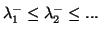
Assume that the eigenvalues of are ordered by magnitude:
.
Assume that the eigenvalues of are ordered by magnitude:
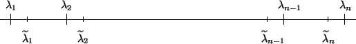
A similar labeling is assumed for the approximations  .
.
As has been mentioned before, the
Ritz values approximate eigenvalues of a Hermitian
matrix ``inside out,'' in the sense that the rightmost eigenvalues
are approximated from below and the leftmost ones are approximated
from above, as is illustrated in the following diagram.
This principle can be applied to harmonic Ritz values: since these
are the result of an orthogonal projection method applied to ,
it follows that the harmonic Ritz eigenvalues  obtained from
the process will approximate corresponding eigenvalues
obtained from
the process will approximate corresponding eigenvalues
 of in an inside-out fashion.
For positive eigenvalues we have,
of in an inside-out fashion.
For positive eigenvalues we have,
Observe that the largest positive eigenvalues are now approximated
from above, in contrast with the standard orthogonal projection
methods. These types of techniques were popular a few decades ago as
a strategy for obtaining intervals that were certain to contain a
given eigenvalue. In fact, as was shown in [349], the Ritz
values together with the harmonic Ritz values form the so-called
Lehmann intervals, which have nice inclusion properties for
eigenvalues of . In a sense, they provide the optimal information
for eigenvalues of that one can derive from a given Krylov subspace.
For example, a lower and upper bound to the
(algebraically) largest positive
eigenvalue can be obtained by using an
orthogonal projection method and a harmonic projection method,
respectively.
We conclude our discussion on harmonic Ritz values with the observation
that they can be computed also for the shifted matrix  , so that
one can force the approximations to improve for eigenvalues close to
, so that
one can force the approximations to improve for eigenvalues close to  .
.
We must be cautious when applying this principle for negative
eigenvalues that the order is reversed. Therefore, we label positive
and negative eigenvalues separately. The above inequalities must be
reversed for the negative eigenvalues, labeled from the
(algebraically) smallest to the largest negative eigenvalues
(
 ). The result is summarized in the
following diagram.
). The result is summarized in the
following diagram.
Assume for simplicity that is SPD and
define:
with
 . Then the Courant characterization
becomes,
. Then the Courant characterization
becomes,
Next: Refined Projection Methods.
Up: Basic Ideas Y. Saad
Previous: Oblique Projection Methods.
Contents
Index
Susan Blackford
2000-11-20