Next: Software Availability
Up: Golub-Kahan-Lanczos Method
Previous: Golub-Kahan-Lanczos Bidiagonalization Procedure.
Contents
Index
From equations (6.7), (6.8), and
(6.9), we have
We note that  is symmetric and tridiagonal,
since
is symmetric and tridiagonal,
since  is bidiagonal.
Comparing to equation (4.10), we see that
Algorithm 6.1
computes the same information as
Lanczos (Algorithm 4.6)
applied to the Hermitian matrix
is bidiagonal.
Comparing to equation (4.10), we see that
Algorithm 6.1
computes the same information as
Lanczos (Algorithm 4.6)
applied to the Hermitian matrix  .
Conversely, if we apply Lanczos to
.
Conversely, if we apply Lanczos to  to get a tridiagonal
matrix
to get a tridiagonal
matrix
 , then can be obtained by taking the
upper triangular Cholesky factor of
, then can be obtained by taking the
upper triangular Cholesky factor of  .
.
Similarly, one gets
Again,  is symmetric and tridiagonal.
So again comparing to equation (4.10), we see that
Algorithm 6.1
computes the same information as
Lanczos (Algorithm 4.6)
applied to the Hermitian matrix
is symmetric and tridiagonal.
So again comparing to equation (4.10), we see that
Algorithm 6.1
computes the same information as
Lanczos (Algorithm 4.6)
applied to the Hermitian matrix  .
Conversely, if we apply Lanczos to to get a tridiagonal
matrix
.
Conversely, if we apply Lanczos to to get a tridiagonal
matrix
 , then can be obtained by taking the
upper triangular Cholesky factor
, then can be obtained by taking the
upper triangular Cholesky factor  of
of  , where
  is
the identity matrix with its columns in reverse order
(so that is gotten by reversing the order of the rows
and then the columns of ), and then
is
the identity matrix with its columns in reverse order
(so that is gotten by reversing the order of the rows
and then the columns of ), and then  .
.
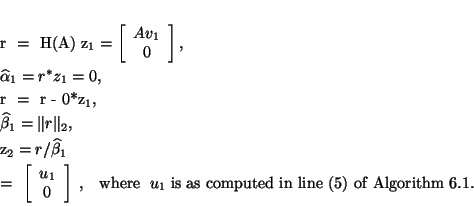
Finally, suppose one applies Lanczos (Algorithm 4.6)
to  with the special starting vector
to generate the Lanczos vectors
 The first step of Algorithm 4.6 yields
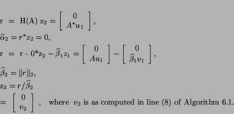
The next step of Algorithm 4.6 yields
Continuing in this fashion, we see that two steps of
Algorithm 4.6 compute the same information
as one step of Algorithm 6.1:
However, Algorithm 4.6 does twice as many matrix-vectors
multiplications by  and
and  as Algorithm 6.1
(half of them by zero vectors), so that
Algorithm 6.1 will generally use half the time and space.
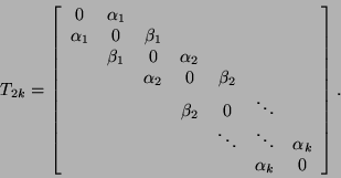
Conversely, if Lanczos is applied to to obtain a
tridiagonal matrix , then will have zeros on its diagonal,
and the off-diagonal entries will be identical to the nonzero entries
of (notation from equation (6.4)):
as Algorithm 6.1
(half of them by zero vectors), so that
Algorithm 6.1 will generally use half the time and space.
Conversely, if Lanczos is applied to to obtain a
tridiagonal matrix , then will have zeros on its diagonal,
and the off-diagonal entries will be identical to the nonzero entries
of (notation from equation (6.4)):
Because of these equivalences, all the algorithmic variations
and convergence properties of Lanczos from §4.4 apply to
Algorithm 6.1.
Next: Software Availability
Up: Golub-Kahan-Lanczos Method
Previous: Golub-Kahan-Lanczos Bidiagonalization Procedure.
Contents
Index
Susan Blackford
2000-11-20