This algorithm again follows the merge strategy and is motivated by the fact that d compare-exchanges in the d different directions of the hypercube result in an almost-sorted list. Global order is defined via ringpos, that is, the list will end up sorted on an embedded ring in the hypercube. After the d compare-exchange stages, the algorithm switches to a simple mopping-up stage which is specially designed for almost-sorted lists. This stage is optimized for moving relatively few items quickly through the machine and amounts to a parallel bucket brigade algorithm. Details and a specification of the parallel shellsort algorithm can be found in Chapter 18 of [Fox:88a].
It turns out that the mop-up algorithm takes advantage of the MIMD nature of the machine and that this characteristic is crucial to its speed. Only the few items which need to be moved are examined and processed. The bitonic algorithm, on the other hand, is natural for a SIMD machine. It involves much extra work in order to handle the worst case, which rarely occurs.
We refer to this algorithm as shellsort ([Shell:59a], [Knuth:73a] pp. 84-5, 102-5) or a diminishing increment algorithm. This is not because it is a strict concurrent implementation of the sequential namesake, but because the algorithms are similar in spirit. The important feature of Shellsort is that in early stages of the sorting process, items take very large jumps through the list reaching their final destinations in few steps. As shown in Figure 12.31, this is exactly what occurs in the concurrent algorithm.
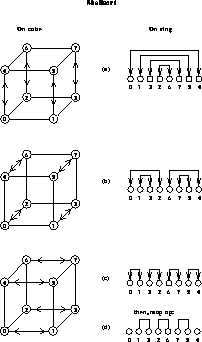
Figure 12.31: The Parallel Shellsort on a d=3 Hypercube. The left side
shows what the algorithm looks like on the cube, the right shows the
same when the cube is regarded as a ring.
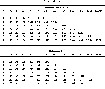
The algorithm was implemented and tested with the same data as the bitonic case. The timings appear in Table 12.3 and are also shown graphically in Figure 12.32. This algorithm is much more efficient than the bitonic algorithm, and offers the prospect of reasonable efficiency at large d. The remaining inefficiency is the result of both communication overhead and algorithmic nonoptimality relative to quicksort. For most list sizes, the mop-up time is a small fraction of the total execution time, though it begins to dominate for very small lists on the largest machine sizes.
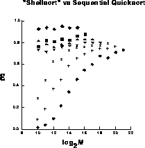
Figure: The Efficiency of the Shellsort Algorithms Versus List Size
for Various Size Hypercubes. The labelling of curves and axes is as
in Figure 12.30.