Inexact Rational Krylov Method

In this section, we combine the ideas of the inexact Cayley transformation, the (Jacobi) Davidson method, and the rational Krylov method. Roughly speaking, we still have the same method as the inexact Cayley transform Arnoldi method or the preconditioned Lanczos method, with the only difference that the zero $\nu$ and the pole $\mu$ may be updated on each iteration. As with the preconditioned Lanczos method, the Ritz vectors are computed from the Hessenberg matrices. In addition, the Ritz values are also computed from the recurrence relation.

We now discuss the method in detail, using the algorithm of the rational Krylov method, designed for the inexact Cayley transforms, given below.

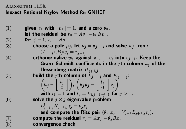
Let us analyze this algorithm step by step. The solution of the linear system leads to the relations (11.2) where $y_j = x_{j-1}$ is a Ritz vector and $\nu_j$ is the associated Ritz value $\theta_{j-1}$ from the previous iteration, such that the right-hand side is the residual $r_{j-1} = A x_{j-1} - \theta_{j-1} B x_{j-1}$. Since $x_{j-1} = V_j L_{j,j-1} z_{j-1}$, we can also write $x_{j-1}=V_j t_j$, where $t_j$ is called the continuation vector. After the Gram-Schmidt orthogonalization, we have $w_j = V_{j+1} h_j$, so we can rewrite (11.2) as

$$A V_{j+1} \left( h_j - \left[\begin{array}{c} t_j \\ 0 \end{... ...gin{array}{c} t_j \\ 0 \end{array}\right] \nu_j \right) - s_j.$$

Collecting all equations for $j=1,\ldots,k$ we have

$$A V_{k+1} L_{k+1,k} = B V_{k+1} K_{k+1,k} - S_k \ ,$$ (277)

which is another way of writing (11.3). Note that when $S_k$ is omitted from this equation, we obtain the usual rational Krylov subspace (RKS) recurrence relation. Also in this case, $L_{k+1,k}$ and $K_{k+1,k}$ are upper Hessenberg matrices and $L_{k+1,k}$ has full rank. Let $L_{k+1,k}^{\dagger}$ denote the generalized Moore-Penrose inverse of $L_{k+1,k}$. With $E_k = S_k L_{k+1,k}^{\dagger} V_{k+1}^{\ast}$, we can also write

$$(A + E_k) V_{k+1} L_{k+1,k} = B V_{k+1} K_{k+1,k},$$ (278)

which corresponds to (11.4). In other words, the RKS coefficient matrices $L_{k+1,k}$ and $K_{k+1,k}$ and the vectors $V_{k+1}$ can be considered as having been computed by the exact rational Krylov method applied to the perturbed problem $(A + E_k) u = \eta B u$. Similar to the term ``inexact'' Cayley transform, we talk about ``inexact'' rational Krylov method.

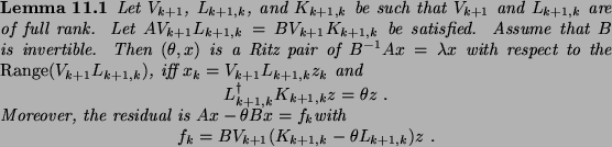
Before we continue, we must give some properties of the exact rational Krylov method. The following lemma explains how to compute Ritz values in the rational Krylov method.

As with the (Jacobi) Davidson method, the RKS method applies an inexact Cayley transform to a vector. The difference lies in the way the Ritz pairs are computed. In the (Jacobi) Davidson method, the Ritz pairs result from a Galerkin projection of $Ax = \lambda Bx$ on the subspace. In the RKS method, the Ritz pairs are computed from the recurrence relation using Lemma 11.1, assuming that $E_k=0$.

With the inexact Cayley transform, the transformation can be a large perturbation of the exact Cayley transform, but can still be used to compute one eigenpair, when $\nu$ is well chosen. The same is true here. The inexact rational Krylov method delivers an $S_k$ (or $E_k$) that is not random but small in the direction of the desired eigenpair, as long as the various parameters are properly set.

A Ritz pair $(\theta,x)$ computed by Algorithm 11.4 produces residual

$$(A + E_k) x - \theta B x = f_k$$

defined by Lemma 11.1. The residual related to the original problem can be written as

$$A x - \theta B x = f_k - E_k x$$

or, following (11.6),

$$A x - \theta B x = f_k -S_k z \ .$$

In order to have small residuals, $E_k x = S_k z$ must tend to zero. Mathematical arguments for the convergence of the inexact rational Krylov
method have been given by Lehoucq and Meerbergen [291] and De Samblanx [109]. We just give a summary of the theory and some numerical results. In [291] and [109], mathematical and heuristical arguments are given that $S_j z_j \approx s_j$ such that, with $\Vert s_j\Vert \leq \tau \Vert r_{j-1}\Vert$ (see §11.2.2), the residual satisfies the recurrence relation

$$\Vert r_j\Vert \approx \Vert f_j\Vert + \tau \Vert r_{j-1}\Vert \ .$$

When the term $f_j$ is dominant to $S_j z_j$ for $j=1,\ldots,k$, then the convergence is dominated by the convergence of the exact rational Krylov process: $A x - \theta B x \approx f_j$. When the second term is dominant, we have $\Vert r_j\Vert \approx \tau^j \Vert r_0\Vert$; i.e., $r_j$ converges towards zero with convergence ratio $\tau$.

• If the underlying exact rational Krylov method converges linearly with a convergence ratio $\rho$ such that $\Vert f_{k+1}\Vert \leq \rho \Vert f_k\Vert$ and if a relative residual tolerance $\tau$ is used for the solution of the linear systems, the effective convergence ratio is approximately $\max(\rho,\tau)$. Linear and superlinear convergence are obtained when $\mu_j$ is constant for all $j$.

• When $\mu_j=\theta_{j-1}$ on each iteration as in the Davidson or Jacobi-Davidson method and $\nu_j=\theta_{j-1}+\epsilon_{j-1}$ (see §11.2.5), then the convergence is quadratic. The term $f_j$ converges quadratically to zero, whereas the second term converges linearly, when $\tau$ does not depend on $j$. Typically, the convergence has a quadratic behavior until $S_j z_j$ becomes the dominant term in $r_j$. From then on, the convergence becomes linear with convergence ratio $\tau$. In practice, it is advised to pick $\tau$ proportional to $\Vert r_j\Vert$ in order to preserve the quadratic convergence. With $\tau_j = \varrho \Vert r_{j-1}\Vert$, we obtain that
  
  $$\Vert r_j\Vert \approx \Vert f_j\Vert + \varrho \Vert r_{j-1}\Vert^2,$$
  
  
  which shows quadratic convergence of the second term.