


Next: Transformation to Linear Form
Up: Quadratic Eigenvalue Problems Z. Bai,
Previous: Quadratic Eigenvalue Problems Z. Bai,
Contents
Index
Introduction
In this section, we consider the quadratic
eigenvalue problem (QEP) of the form
 |
(245) |
where  , and
, and  are given matrices of size
  .
The nontrivial
.
The nontrivial  -vectors
  ,
,  , and the corresponding scalars
 are the right, left eigenvectors, and eigenvalues, respectively.
The matrix function
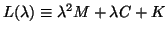 is a special case of a matrix polynomial, or a -matrix;
see, for example, [187,284,194].
In this case, it is a -matrix of degree 2.
The matrix function
is a special case of a matrix polynomial, or a -matrix;
see, for example, [187,284,194].
In this case, it is a -matrix of degree 2.
The matrix function  is said to be regular
if
is said to be regular
if
 is not identical to zero for all . Otherwise, it is called
singular.
is not identical to zero for all . Otherwise, it is called
singular.
An important special case of the quadratic eigenvalue problem is when
 |
(246) |
These matrices are sometimes called mass, damping, and
stiffness matrices, respectively, referring to their origin in mechanical
engineering models; see, for instance, [145].
In some problems, the stiffness matrix  is only semi-positive definite.
In this case, we may consider a shifted QEP to be discussed in
§9.2.3.
is only semi-positive definite.
In this case, we may consider a shifted QEP to be discussed in
§9.2.3.
One of the factors that makes the QEP
different from standard eigenproblems  , or generalized
eigenproblems
, or generalized
eigenproblems
 ,
is that there are
,
is that there are  eigenvalues for QEP, with at most
right (and left) eigenvectors. Of course, in an -dimensional space
the right (and left) eigenvectors no longer form an independent set.
This is illustrated by the following simple example. The triplet
eigenvalues for QEP, with at most
right (and left) eigenvectors. Of course, in an -dimensional space
the right (and left) eigenvectors no longer form an independent set.
This is illustrated by the following simple example. The triplet
has  different (but pairwise conjugate) eigenvalues
(rounded to five decimals):
different (but pairwise conjugate) eigenvalues
(rounded to five decimals):
The associated eigenvectors (normalized so that the first coordinate is equal
to 1) are:
The four eigenvectors are obviously dependent, but, in actual
problems, each of them may represent a relevant state of the system.
One has to be careful with Rayleigh quotients for quadratic eigenproblems.
Indeed, given as a right eigenvector for the
QEP (9.1), i.e.,
one can form a quadratic Rayleigh quotient:
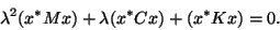 |
(247) |
However, this equation has two roots; one of the roots is an
eigenvalue, the other root may be a spurious one.
For instance, if we compute the quadratic Rayleigh quotient for our
example, with
 ,
then clearly, the pair
satisfies equation (9.3).
If we solve equation (9.3), then we find the two roots
,
then clearly, the pair
satisfies equation (9.3).
If we solve equation (9.3), then we find the two roots
 ,
,
 . We see that
  is recovered (by
  ) and the other root has no meaning for the given
QEP.
) and the other root has no meaning for the given
QEP.
In an effort to decide which of the two is the desired one and which is the
spurious one, one could compute the residual vector
and this leads to
 ,
,
 , which, in this case, clearly points out that
 is not an eigenvalue. We cannot exclude the possibility that in contrived examples,
one might make a wrong choice, which may lead to a delay in a specific
iterative solution method.
is not an eigenvalue. We cannot exclude the possibility that in contrived examples,
one might make a wrong choice, which may lead to a delay in a specific
iterative solution method.
For more general matrices, we can have defectiveness, as for the standard
eigenproblems, which means that there is not necessarily a complete set of
eigenvectors. In the next section, we will relate the QEP to a generalized
standard problem, which helps to shed more light on this matter.
Next: Transformation to Linear Form
Up: Quadratic Eigenvalue Problems Z. Bai,
Previous: Quadratic Eigenvalue Problems Z. Bai,
Contents
Index
Susan Blackford
2000-11-20