Next: Numerical Stability and Conditioning
Up: A Brief Tour of
Previous: A Brief Tour of
Contents
Index
Introduction
Let  be a square
  by matrix,
 a nonzero by 1 vector (a column vector),
and
a nonzero by 1 vector (a column vector),
and  a scalar, such that
 |
(1) |
Then is called an eigenvalue of , and
is called a (right) eigenvector. Sometimes we refer
to  as an eigenpair.
We refer the reader to the list of symbols and acronyms on page
as an eigenpair.
We refer the reader to the list of symbols and acronyms on page ![[*]](http://www.netlib.org/utk/icons/crossref.png) ;
we will use the notation listed there freely throughout the text.
;
we will use the notation listed there freely throughout the text.
In this chapter we introduce and classify all the eigenproblems
discussed in this book, describing their basic
mathematical properties and interrelationships.
Eigenproblems
can be defined by a single square matrix as in
(2.1), by a nonsquare matrix ,
by 2 or more square or rectangular matrices, or even by
a matrix function of .
We use the word ``eigenproblem'' in order to encompass computing
eigenvalues, eigenvectors, Schur decompositions, condition numbers
of eigenvalues, singular value and vectors, and yet other
terms to be defined below. After reading this chapter the
reader should be able to recognize the mathematical types
of many eigenproblems, which are essential to picking
the most effective algorithms. Not recognizing the right
mathematical type of an eigenproblem can lead to using
an algorithm that might not work at all or that might
take orders of magnitude more time and space than a more specialized
algorithm.
To illustrate the sources and interrelationships of these eigenproblems,
we have a set of related examples for each one.
The sections of this chapter are organized to correspond
to the next six chapters of this book:
- Section 2.2:
- Hermitian eigenproblems (HEP) (Chapter 4).
This corresponds to
 as in
(2.1), where is Hermitian, i.e.,
as in
(2.1), where is Hermitian, i.e.,  .
.
- Section 2.3:
- Generalized Hermitian eigenproblems (GHEP) (Chapter 5).
This corresponds to
 , where and
  are
Hermitian and is positive definite (has all positive eigenvalues).
are
Hermitian and is positive definite (has all positive eigenvalues).
- Section 2.4:
- Singular value decomposition (SVD) (Chapter 6).
Given any rectangular matrix ,
this corresponds to finding the eigenvalues and eigenvectors
of the Hermitian matrices
 and
and  .
.
- Section 2.5:
- Non-Hermitian eigenproblems (NHEP) (Chapter 7).
This corresponds to
as in
(2.1), where is square but otherwise general.
- Section 2.6:
- Generalized non-Hermitian eigenproblems (GNHEP) (Chapter 8).
This corresponds to
.
We will first treat the most common case
of the regular generalized eigenproblem,
which occurs when and are square and
 is nonsingular for some choice
of scalars
is nonsingular for some choice
of scalars  and
and  .
We will also discuss the singular case.
.
We will also discuss the singular case.
- Section 2.7:
- Nonlinear eigenproblems (Chapter 9).
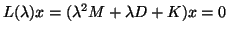
The simplest case of this is the quadratic eigenvalue problem
 and includes
higher degree polynomials as well.
We also discuss maximizing a real function
and includes
higher degree polynomials as well.
We also discuss maximizing a real function  over the
space of
over the
space of  by orthonormal matrices; this includes eigenproblems
as a special case as well as much more complicated problems such
as simultaneously reducing two or more symmetric matrices to diagonal
form as nearly as possible using the same set of approximate eigenvectors
for all of them.
by orthonormal matrices; this includes eigenproblems
as a special case as well as much more complicated problems such
as simultaneously reducing two or more symmetric matrices to diagonal
form as nearly as possible using the same set of approximate eigenvectors
for all of them.
Bai's note: this section is not necessary, there are not
much we can/need to say.
in the singular case is discussed in
Chap 8.
[Sec ]
More generalized eigenproblems (Chapter 9).
This chapter includes several cases.
First, we discuss
in the singular case,
i.e. when the eigenvalues are not continuous functions.
Second we discuss polynomial eigenproblems
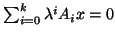 . When
  we get
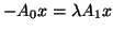 which corresponds to cases considered before.
Third, we consider the fully nonlinear case
which corresponds to cases considered before.
Third, we consider the fully nonlinear case
 , where
can depend on in any continuous way. When
, where
can depend on in any continuous way. When  is a polynomial in we get the previous case.
All the eigenproblems described above arise naturally in
applications arising in science and engineering.
In each section we also show how one can recognize and solve
closely related eigenproblems (for example, GEHPs,
where
 is
positive definite instead of ).
Chapters are presented in roughly increasing order
of generality and complexity.
For example, the HEP
is
clearly a special case of the GHEP
, because we can set
is
positive definite instead of ).
Chapters are presented in roughly increasing order
of generality and complexity.
For example, the HEP
is
clearly a special case of the GHEP
, because we can set  . It is also a special case
of the NHEP, because we can ignore 's
Hermitian symmetry and treat it as a general matrix.
. It is also a special case
of the NHEP, because we can ignore 's
Hermitian symmetry and treat it as a general matrix.
In general, the larger or more difficult an eigenvalue
problem, the more important it is to use an algorithm that
exploits as much of its mathematical structure as possible
(such as symmetry or sparsity).
For example, one can use
algorithms for non-Hermitian problems to treat Hermitian ones, but
the price is a large increase in time, storage, and possibly lower
accuracy.
Each section from 2.2 through 2.6 is
organized as follows.
- The basic definitions of eigenvalues and eigenvectors will be given.
- Eigenspaces will be defined.
A subspace
 is defined as
the space
is defined as
the space
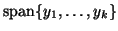 spanned by a chosen
set of vectors
spanned by a chosen
set of vectors
 ;
i.e., is the set of all linear combinations of
.
Eigenspaces are (typically) spanned by a subset of eigenvectors
and may be called invariant subspaces, deflating subspaces,
or something else depending on the type of eigenproblem.
;
i.e., is the set of all linear combinations of
.
Eigenspaces are (typically) spanned by a subset of eigenvectors
and may be called invariant subspaces, deflating subspaces,
or something else depending on the type of eigenproblem.
- Equivalences will be defined; these are transformations
(such as changing to
 ) that leave the eigenvalues unchanged
and can be used to compute a ``simpler representation''
of the eigenproblem.
Depending on the situation, equivalences are also called similarities
or congruences.
) that leave the eigenvalues unchanged
and can be used to compute a ``simpler representation''
of the eigenproblem.
Depending on the situation, equivalences are also called similarities
or congruences.
- Eigendecompositions will be defined; these are commonly computed
``simpler representations.''
- Conditioning will be discussed.
A condition number
measures how sensitive the eigenvalues
and eigenspaces of are to small changes in .
These small changes could arise from roundoff or other unavoidable
approximations made by the algorithm, or from uncertainty in the entries
of .
One can get error bounds on computed eigenvalues and eigenspaces by multiplying
their condition numbers by a bound on the change in .
For more details on how condition numbers are used to get error
bounds, see §2.1.1.
An eigenvalue or eigenspace is called well-conditioned if
its error bound is acceptably small for the user (this obviously depends
on the user), and ill-conditioned
if it is much larger.
Conditioning is important not just to interpret the computed results of
an algorithm, but to choose the information to be computed. For example,
different representations of the same eigenspace may have very different
condition numbers, and it is often better to compute the better conditioned
representation. Conditioning is discussed in more detail in each chapter,
but the general results are summarized here.
- Different ways of specifying an eigenproblem are listed.
The most expensive eigenvalue
problem is to ask for all eigenvalues and eigenvectors of .
Since this is often too expensive in time and space, users frequently
ask for less information, such as the largest 10 eigenvalues and
perhaps their eigenvectors.
(Note that if is sparse, typically
the eigenvectors are dense, so storing all the eigenvectors can take
much more memory than storing .) Also, some eigenproblems
for the same matrix may be much better conditioned than others,
and these may be preferable to compute.
- Related eigenproblems are discussed. For example, if it is possible
to convert an eigenproblem into a simpler and cheaper special case, this is shown.
- The vibrational analysis of the
mass-spring system
shown in Figure 2.1
is used
to illustrate the source and formulation of each eigenproblem.
Figure 2.1:
Damped, vibrating mass-spring system.
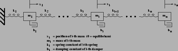 |
Newton's law  applied to this vibrating mass-spring
system yields
applied to this vibrating mass-spring
system yields
where the first term on the left-hand side
is the force on mass  from spring ,
the second term is the force on mass from spring
from spring ,
the second term is the force on mass from spring  ,
and the third term is the force on mass from damper .
In matrix form, these equations can be written as
,
and the third term is the force on mass from damper .
In matrix form, these equations can be written as
where
 ,
,
 , and
, and
We assume all the masses  are positive.
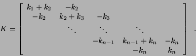
 is called the mass matrix, is the damping matrix,
and
is called the mass matrix, is the damping matrix,
and  is the stiffness matrix. All three matrices are
symmetric. They are also positive definite (have all positive eigenvalues)
when the ,
is the stiffness matrix. All three matrices are
symmetric. They are also positive definite (have all positive eigenvalues)
when the ,  , and
, and  are positive, respectively.
This differential equation becomes an eigenvalue problem
by seeking solutions of the form
are positive, respectively.
This differential equation becomes an eigenvalue problem
by seeking solutions of the form
 , where
is a constant scalar and is a constant vector,
both of which are determined by solving appropriate eigenproblems.
, where
is a constant scalar and is a constant vector,
both of which are determined by solving appropriate eigenproblems.
Electrical engineers analyzing linear circuits arrive at an analogous equation
by applying Kirchoff's and related laws instead of Newton's law. In this case
represents branch currents, represent inductances,
represents resistances, and represents admittances (reciprocal
capacitances).
Chapter 9 on nonlinear eigenproblems is organized differently,
according to the structure of the specific nonlinear problems discussed.
Finally, Chapters 10 and
11 treat issues common to
many or all of the above eigenvalue problems.
Chapter 10 treats data structures,
algorithms, and software for
sparse matrices, especially sparse linear solvers, which often are the
most time-consuming part of an eigenvalue algorithm.
Chapter 11 treats preconditioning techniques or methods for
converting an eigenproblem into a simpler one. Some preconditioning techniques
are well established; others are a matter of current research.
Subsections
Next: Numerical Stability and Conditioning
Up: A Brief Tour of
Previous: A Brief Tour of
Contents
Index
Susan Blackford
2000-11-20