


We have seen many times that parallel computing involves breaking problems into parts which execute concurrently. In the simple regular problems seen in the early chapters, especially Chapters 4 and 6, it was usually reasonably obvious how to perform this breakup to optimize performance of the program on a parallel machine. However, in Chapter 9 and even more so in Chapter 12, we will find that the nature of the parallelism is as clear as before, but that it is nontrivial to implement efficiently.
Irregular loosely synchronous problems consist of a collection of
heterogeneous tasks communicating with each other at the
macrosynchronization points characteristic of this problem class. Both
the execution time per task and amount and pattern of communication can
differ from task to task. In this section, we describe and compare
several approaches to this problem. We note that formally this is a
very hard-so-called NP-complete-optimization problem. With
 tasks running on
  processors we
cannot afford to examine every one of the
processors we
cannot afford to examine every one of the 
 assignments of tasks to processors.
Experience has shown that this problem is easier than one would have
thought-partly at least because one does not require the exactly
optimal assignment. Rather, a solution whose execution time is, say,
within 10% of the optimal value is quite acceptable. Remember, one
has probably chosen to ``throw away'' a larger fraction than this of
the possible MPP performance by using a high-level language such as
Fortran or C on the node (independent of any parallelism issues). The
physical optimization
methods described in Section 11.3 and more problem-specific
heuristics have shown themselves very suitable for
this class of approximate optimization [Fox:91j;92i].
In 1985, at a DOE contract renewal review at Caltech,
we thought that this load balancing issue would be a major and perhaps
the key stumbling block for parallel computing. However, this is not
the case-it is a hard and important problem, but for loosely
synchronous problems it can be solved straightforwardly
[Barnard:93a], [Fox:92c;92h;92i],
[Fox:92h] [Mansour:92d]. Our approach to
this uses physical analogies and stems in fact from dinner
conversations between Fox and David Jefferson, a collaborator from
UCLA, at this meeting
[Fox:85k;86a;88e;88mm]. An
interesting computer science challenge is to understand why the
NP-complete load-balancing problem appears ``easier
in practice'' than the Travelling Salesman Problem, which is the
generic NP-complete optimization problem. We will return to this
briefly in Section 11.3, but note that the ``shape of the
objection function'' (in physics language, the ``energy landscape'')
illustrated in Figure 11.1 appears critical. Load-balancing
problems appear to fall into the ``easy class'' of NP-complete
optimization problems with the landscape of Figure 11.1(a).
The methods discussed in the following are only a sample of the many
effective approaches developed recently: [Barhen:88a],
[Berger:87a], [Chen:88a], [Chrisochoides:91a],
[Ercal:88a], [Ercal:88b],
[Farhat:88a;89b], [Fox:88nn],
[Hammond:92b], [Houstis:90a], [Livingston:88a],
[Miller:92a], [Nolting:91a], [Teng:91a],
[Walker:90b]. The work of Simon [Barnard:93a],
[Pothen:90a], [Simon:91b], [Venkatakrishnan:92a] on
recursive spectral bisection-a method with similarities to the eigenvector recursive bisection (ERB) method mentioned later-has
been particularly successful.
assignments of tasks to processors.
Experience has shown that this problem is easier than one would have
thought-partly at least because one does not require the exactly
optimal assignment. Rather, a solution whose execution time is, say,
within 10% of the optimal value is quite acceptable. Remember, one
has probably chosen to ``throw away'' a larger fraction than this of
the possible MPP performance by using a high-level language such as
Fortran or C on the node (independent of any parallelism issues). The
physical optimization
methods described in Section 11.3 and more problem-specific
heuristics have shown themselves very suitable for
this class of approximate optimization [Fox:91j;92i].
In 1985, at a DOE contract renewal review at Caltech,
we thought that this load balancing issue would be a major and perhaps
the key stumbling block for parallel computing. However, this is not
the case-it is a hard and important problem, but for loosely
synchronous problems it can be solved straightforwardly
[Barnard:93a], [Fox:92c;92h;92i],
[Fox:92h] [Mansour:92d]. Our approach to
this uses physical analogies and stems in fact from dinner
conversations between Fox and David Jefferson, a collaborator from
UCLA, at this meeting
[Fox:85k;86a;88e;88mm]. An
interesting computer science challenge is to understand why the
NP-complete load-balancing problem appears ``easier
in practice'' than the Travelling Salesman Problem, which is the
generic NP-complete optimization problem. We will return to this
briefly in Section 11.3, but note that the ``shape of the
objection function'' (in physics language, the ``energy landscape'')
illustrated in Figure 11.1 appears critical. Load-balancing
problems appear to fall into the ``easy class'' of NP-complete
optimization problems with the landscape of Figure 11.1(a).
The methods discussed in the following are only a sample of the many
effective approaches developed recently: [Barhen:88a],
[Berger:87a], [Chen:88a], [Chrisochoides:91a],
[Ercal:88a], [Ercal:88b],
[Farhat:88a;89b], [Fox:88nn],
[Hammond:92b], [Houstis:90a], [Livingston:88a],
[Miller:92a], [Nolting:91a], [Teng:91a],
[Walker:90b]. The work of Simon [Barnard:93a],
[Pothen:90a], [Simon:91b], [Venkatakrishnan:92a] on
recursive spectral bisection-a method with similarities to the eigenvector recursive bisection (ERB) method mentioned later-has
been particularly successful.
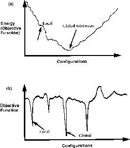
Figure 11.1: Two Possible ``Energy Landscapes'' for an Optimization
Problem
A few general remarks are necessary; we use the phrases ``load balancing'' and ``data decomposition'' interchangeably. One needs both ab initio and dynamic distribution and redistribution of data on the parallel machine. We also can examine load balancing at the level of data or of tasks that encapsulate the data and algorithm. In elegant (but currently inefficient) software models with one datum per task, these formulations are equivalent. Our examples will do load balancing at the level of data values, but the task and data distribution problems are essentially equivalent.
Our methods are applicable to general loosely synchronous problems and indeed can be applied to arbitrary problem classes. However, we will choose a particular finite-element problem to illustrate the issues where one needs to distribute a mesh, such as that illustrated in Figure 11.2. Each triangle or element represents a task which communicates with its neighboring three triangles. In doing, for example, a simulation of fluid flow on the mesh, each element of the mesh communicates regularly with its neighbors, and this pattern may be repeated thousands of times.
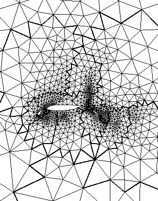
Figure 11.2: An Unstructured Triangular Mesh Surrounding a Four-Element
Airfoil. The mesh is distributed among 16 processors, with divisions
shown by heavy lines.
We may classify load-balancing strategies into four broad types, depending on when the optimization is made and whether the cost of the optimization is included in the optimization itself:\
Koller calls these problems adiabatic [Fox:90nn], using a physical analogy where the load balancer can be viewed as a heatbath keeping the problem in equilibrium. In adiabatic systems, changes are sufficiently slow that the heatbath can ``keep up'' and the system evolves from equilibrium state to equilibrium state.
If the mesh is solution-adaptive, that is, if the mesh, and hence the load-balancing problem, change discretely during execution of the code, then it is most efficient to decide the optimal mesh distribution in parallel. In this section, three parallel algorithms, orthogonal recursive bisection (ORB), eigenvector recursive bisection (ERB) and a simple parallelization of simulated annealing (SA) are discussed for load-balancing a dynamic unstructured triangular mesh on 16 processors of an nCUBE machine.
The test problem is a solution-adaptive Laplace solver, with an initial mesh of 280 elements, refined in seven stages to 5772 elements. We present execution times for the solver resulting from the mesh distributions using the three algorithms, as well as results on imbalance, communication traffic, and element migration.
In this section, we shall consider the quasi-dynamic case with observations on the time taken to do the load balancing that bear on the dynamic case. The testbed is an unstructured-mesh finite-element code, where the elements are the atoms of the problem, which are to be assigned to processors. The mesh is solution-adaptive, meaning that it becomes finer in places where the solution of the problem dictates refinement.
We shall show that a class of finite-element applications share common load-balancing requirements, and formulate load balancing as a graph-coloring problem. We shall discuss three methods for solving this graph-coloring problem: one based on statistical physics, one derived from a computational neural net, and one cheap and simple method.
We present results from running these three load-balancing methods, both in terms of the quality of the graph-coloring solution (machine-independent results), and in terms of the particular machine (16 processors of an nCUBE) on which the test was run.