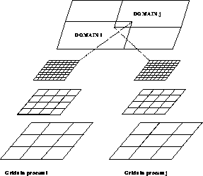
Figure 9.18: Use of Adaptive Multigrid for Concurrency


The same structure that made the multigrid code adaptive allows us to parallelize it. For now, assume that every process starts out with a copy of the coarsest grid, defined on the whole domain. Each process is assigned a subdomain in which to compute the solution to maximum accuracy. The collection of subdomains assigned to all processes covers the computational domain. Within each process, an adaptive grid structure is constructed so that the finest level at which the solution is needed envelops the assigned subdomain; see Figure 9.18. The set of all grids (in whatever process they reside) forms a tree structure like the one described in the previous section. The same algorithm can be applied to it. Only one addition must be made to the program: overlapping grids on the same level but residing in different processes must communicate in order to interpolate boundary values. This is an operation to be added to the basic library.

Figure 9.18: Use of Adaptive Multigrid for Concurrency
The coarsest grid can often be ignored as far as machine efficiency is concerned. As mentioned in Section 9.7.2, the computations on the coarsest grid are sometimes substantial. In such cases, it is crucial to parallelize the coarsest-grid computations. With relaxation until convergence as the coarsest-grid solver, one could simply divide up the coarsest grid over all concurrent processes. It is more likely, however, that the coarsest-grid computations involve a direct solution method. In this case, the duplicated coarsest grid is well suited as an interface to a concurrent direct solver, because it simplifies the initialization of the coefficient matrix. We refer to Section 8.1 and [Velde:90a] for details on some direct solvers.
The total algorithm, adaptive multigrid and concurrent coarsest grid solver, is heterogeneous: its communication structure is irregular and varies significantly from one part of the program to the next, making the data distribution for optimal load balance difficult to predict. On the coarsest level, we achieve load balance by exploiting the data distribution independence of our linear algebra code; see [Lorenz:92a]. On the finer levels, load balance is obtained by allocating an approximately equal number of finest-grid points to each process.


