We address the following initial-value problem consisting of combinations of
N linear and nonlinear coupled, ordinary differential-algebraic
equations over the interval  :
:
IVP :
:
with unknown state vector  , known external inputs
 , where
  and
and
 are the given initial-value,
derivative vectors, respectively. We will refer to Equation 9.11's
deviation from
are the given initial-value,
derivative vectors, respectively. We will refer to Equation 9.11's
deviation from  as the residuals or residual vector. Evaluating the
residuals means computing
as the residuals or residual vector. Evaluating the
residuals means computing  (``model
evaluation'') for specified arguments
(``model
evaluation'') for specified arguments  ,
,  ,
,  and t.
DASSL's integration algorithm can be used to solve systems fully
implicit in  and
and  and of index zero or one, and
specially structured forms of index two (and higher)
[Brenan:89a, Chapter 5], where the index is the minimum number of times
that part or all of Equation 9.11 must be differentiated with
respect to t in order to express
and of index zero or one, and
specially structured forms of index two (and higher)
[Brenan:89a, Chapter 5], where the index is the minimum number of times
that part or all of Equation 9.11 must be differentiated with
respect to t in order to express  as a continuous function
of
as a continuous function
of  and t [Brenan:89a, page 17].
By substituting a finite-difference approximation  for
for
 , we obtain:
a set of (in general) nonlinear staticized equations. A sequence of
Equation 9.12's will have to be solved, one at each discrete time

 , in the numerical
approximation scheme; neither M nor the
, in the numerical
approximation scheme; neither M nor the  's need be
predetermined. In DASSL, the variable step-size integration algorithm
picks the
's need be
predetermined. In DASSL, the variable step-size integration algorithm
picks the  's as the integration progresses, based on its
assessment of the local error. The discretization operator for
's as the integration progresses, based on its
assessment of the local error. The discretization operator for  ,
,  , varies during the numerical integration process and
hence is subscripted as
, varies during the numerical integration process and
hence is subscripted as  .
.
The usual way to solve an instance of the staticized equations,
Equation 9.12, is via the familiar Newton-Raphson iterative
method (yielding  ):
):
given an initial, sufficiently good approximation  . The
classical method is recovered for
. The
classical method is recovered for  and c = 1, whereas a modified
(damped) Newton-Raphson method results for
and c = 1, whereas a modified
(damped) Newton-Raphson method results for  (respectively,
 ). In the original DASSL algorithm and in Concurrent
DASSL, the Jacobian
). In the original DASSL algorithm and in Concurrent
DASSL, the Jacobian  is
computed by finite differences rather than
analytically; this departure leads in another sense to a modified
Newton-Raphson method even though
is
computed by finite differences rather than
analytically; this departure leads in another sense to a modified
Newton-Raphson method even though  and c = 1 might always
be satisfied. For termination, a limit
and c = 1 might always
be satisfied. For termination, a limit  is imposed; a
further stopping criterion of the form
is imposed; a
further stopping criterion of the form  is also incorporated (see Brenan et al.
[Brenan:89a, pages 121-124]).
is also incorporated (see Brenan et al.
[Brenan:89a, pages 121-124]).
Following Brenan et al., the approximation  is
replaced by a BDF-generated linear approximation,
is
replaced by a BDF-generated linear approximation,  ,
and the Jacobian
,
and the Jacobian
From this approximation, we define  in the intuitive way. We then consider Taylor's Theorem with
remainder, from which we can easily express a forward finite-difference
approximation for each Jacobian column (assuming sufficient smoothness of
in the intuitive way. We then consider Taylor's Theorem with
remainder, from which we can easily express a forward finite-difference
approximation for each Jacobian column (assuming sufficient smoothness of
 ) with a scaled difference of two residual vectors:
By picking  proportional to
  , the
junit vector in the natural basis for
, the
junit vector in the natural basis for  , namely
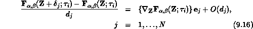
 , Equation 9.15 yields a
first-order-accurate approximation in
, Equation 9.15 yields a
first-order-accurate approximation in  of the jcolumn of the
Jacobian matrix:
of the jcolumn of the
Jacobian matrix:
Each of these N Jacobian-column computations is independent and trivially parallelizable. It's well known, however, that for special structures such as banded and block n-diagonal matrices, and even for general sparse matrices, a single residual can be used to generate multiple Jacobian columns [Brenan:89a], [Duff:86a]. We discuss these issues as part of the concurrent formulation section below.
The solution of the Jacobian linear system of equations is required for each
k-iteration, either through a direct (e.g., LU-factorization) or
iterative (e.g., preconditioned-conjugate-gradient) method. The most
advantageous solution approach depends on N as well as special mathematical
properties and/or structure of the Jacobian matrix  . Together, the inner (linear equation solution) and
outer (Newton-Raphson iteration) loops solve a single
time point; the overall algorithm generates a sequence of solution points
. Together, the inner (linear equation solution) and
outer (Newton-Raphson iteration) loops solve a single
time point; the overall algorithm generates a sequence of solution points
 .
.
In the present work, we restrict our attention to direct, sparse linear algebra as described in [Skjellum:90d], although future versions of Concurrent DASSL will support the iterative linear algebra approaches by Ashby, Lee, Brown, Hindmarsh et al. [Ashby:90a], [Brown:91a]. For the sparse LU factorization, the factors are stored and reused in the modified Newton scenario. Then, repeated use of the old Jacobian implies just a forward- and back-solve step using the triangular factors L and U. Practically, we can use the Jacobian for up to about five steps [Brenan:89a]. The useful lifetime of a single Jacobian evidently depends somewhat strongly on details of the integration procedure [Brenan:89a].