4 The Parallel IFS - Partitioning Concepts

 

 

Each time step of the IFS consists of computations in three different spaces (grid point space, Fourier space and spectral space) and has the following order:

1. computations in grid point space,
2. transition to Fourier space by Fast Fourier Transforms,
3. computations in Fourier space,
4. transition to spectral space by Legendre transforms,
5. computations in spectral space (phase I),
6. computations in spectral space (phase II),
7. transition to Fourier space by inverse Legendre transforms,
8. computations in Fourier space and
9. transition to grid point space by inverse Fourier transforms.

In each of these computational steps complex data dependencies exist in exactly one dimension while the other two dimensions are freely available for parallelisation and vectorisation. Unfortunately, the independent directions vary among the different computational steps. In grid point space, for example, these data dependencies are in the vertical direction without any influence of longitudes and latitudes, while in Fourier space, the data dependencies refer to the longitudinal dimension.

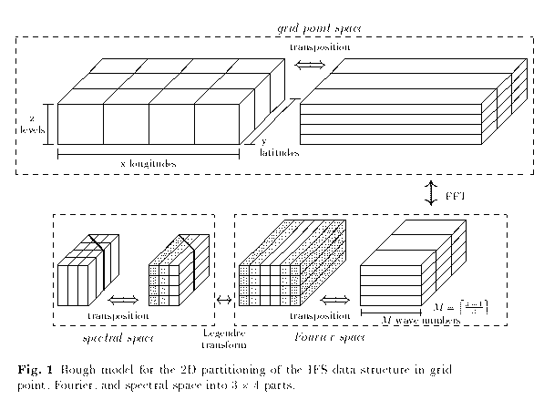
So, in each computational step a partitioning of the data and the computations to processes is possible with respect to two dimensions, providing a high degree of parallelism. The data transposition strategy  [1, 4] allows to utilise this approach efficiently on parallel systems. Its idea is to re-distribute the complete data to the processes (data transposition) at some stages of the algorithm such that the arithmetic computations between two consecutive transpositions can be performed without any interprocess communication: during the corresponding computational step the direction with data dependencies is not partitioned among processes.

Figure 1 shows the structure of the parallel algorithm: here, the data are partitioned among 3 X 4 processes. Transpositions are performed in each data space in order to allow a fully parallelised computational phase without any interprocess communication. The dashed cells in Fourier and spectral space illustrate the data partitioning before and after the Legendre transforms; in Fourier space each process is responsible for two of the indicated process columns (which are in general not adjacent) in order to provide load balanced Legendre transforms.

The usual expression for the size of the IFS data structure is TM Lz, where M is the wave number and z is the number of levels. We investigate TM L31 with M=63, 106, 213. The standard relation between M and the number of grid points in direction of longitudes or latitudes is and (cf. Figure 1). For the present paper we consider the RAPS version 2.0 with full grid and Eulerian treatment of advection. The finest grid size corresponds to a 60 km network on the equator.

 

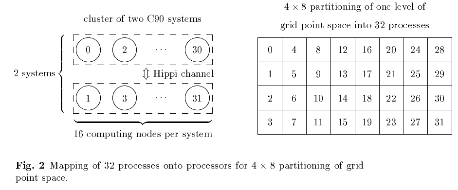
For the mapping of the process structure onto the computing nodes we used a simple mapping function called column-mapping. Here the columns of the process structure are mapped onto the columns of the cluster structure one after the other. Depending on the size of these columns, more than one process column might be mapped onto one cluster column or one process column might be split to several cluster columns. Let and denote the elements of the -process structure or the -cluster structure respectively. The -cluster structure represents a cluster of C90 systems each of which consists of computing nodes. Then the column-mapping is defined by . 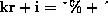We refer to Figure 2 as an example of this mapping.