Linear Equations

 

We use the standard notation for a system of simultaneous linear  equations :
 
where A is the coefficient matrix , b is the right-hand side  , and x is the solution  . In (3.2) A is assumed to be a square matrix of order n, but some of the individual routines allow A to be rectangular. If there are several right-hand sides we write
 
where the columns of B are the individual right-hand sides, and the columns of X are the corresponding solutions. The basic task is to compute X, given A and B.

If A is upper or lower triangular, (3.2) can be solved by a straightforward process of backward or forward substitution. Otherwise, the solution is obtained after first factorizing A as a product of triangular matrices (and possibly also a diagonal matrix or permutation matrix).

The form of the factorization depends on the properties of the matrix A. ScaLAPACK provides routines for the following types of matrices, based on the stated  factorizations:

• general matrices   (LU factorization with partial pivoting)  :
  
  where P is a permutation matrix, L is lower triangular with unit diagonal elements (lower trapezoidal if m > n), and U is upper triangular (upper trapezoidal if m < n).
• symmetric and Hermitian positive definite matrices (Cholesky factorization) :
  
  
  
  where U is an upper triangular matrix and L is lower triangular.
• general band matrices (LU factorization with partial pivoting):
  

  If A is m-by-n with bwl subdiagonals and bwu superdiagonals, the factorization is
  
  where P and Q are permutation matrices and L and U are banded lower and upper triangular matrices, respectively.

• general diagonally dominant-like band matrices  including general tridiagonal matrices (LU factorization without pivoting):
  

  A diagonally dominant-like  matrix is one for which it is known a priori that pivoting for stability is NOT required in the LU factorization of the matrix. Diagonally dominant matrices themselves are examples of diagonally dominant-like matrices.
  

  If A is m-by-n with bwl subdiagonals and bwu superdiagonals, the factorization is
  
  where P is a permutation matrix and L and U are banded lower and upper triangular matrices respectively.

• symmetric and Hermitian positive definite band matrices (Cholesky factorization) :
  
  
  
  where P is a permutation matrix and U and L are banded upper and lower triangular matrices, respectively.
• symmetric and Hermitian positive definite tridiagonal matrices ( factorization):  
  
  
  
  where P is a permutation matrix and U and L are bidiagonal upper and lower triangular matrices respectively.

Note: In the banded and tridiagonal factorizations (PxDBTRF, PxDTTRF, PxGBTRF, PxPBTRF, and PxPTTRF), the resulting factorization is not the same factorization as returned from LAPACK. Additional permutations are performed on the matrix for the sake of parallelism. Further details of the algorithmic implementations can be found in [32].

The factorization for a general diagonally dominant-like  tridiagonal matrix is like that for a general diagonally dominant-like band matrix with bwl = 1 and bwu = 1. Band matrices use the band storage scheme described in section 4.4.3.

While the primary use of a matrix factorization is to solve a system of equations, other related tasks are provided as well. Wherever possible, ScaLAPACK provides routines to perform each of these tasks for each type of matrix and storage scheme (see table 3.6). The following list relates the tasks to the last three characters of the name of the corresponding computational routine:

PxyyTRF:

factorize (obviously not needed for triangular matrices);                                 

PxyyTRS:

use the factorization (or the matrix A itself if it is triangular) to solve (3.3) by forward or backward substitution;                                      

PxyyCON:

estimate the reciprocal of the condition number ; Higham's modification [81] of Hager's method [72] is used to estimate (not provided for band or tridiagonal matrices);               

PxyyRFS:

compute bounds on the error in the computed solution (returned by the PxyyTRS routine), and refine the solution to reduce the backward error (see below) (not provided for band or tridiagonal matrices);               

PxyyTRI:

use the factorization (or the matrix A itself if it is triangular) to compute (not provided for band matrices, because the inverse does not in general preserve bandedness);                   

PxyyEQU:

compute scaling factors to equilibrate  A (not provided for band, tridiagonal, or triangular matrices). These routines do not actually scale the matrices: auxiliary routines PxLAQyy may be used for that purpose -- see the code of the driver routines PxyySVX for sample usage .          

Note that some of the above routines depend on the output of others:

PxyyTRF:

may work on an equilibrated matrix produced by PxyyEQU and PxLAQyy, if yy is one of {GE, PO};

PxyyTRS:

requires the factorization returned by PxyyTRF;

PxyyCON:

requires the norm of the original matrix A and the factorization returned by PxyyTRF;

PxyyRFS:

requires the original matrices A and B, the factorization returned by PxyyTRF, and the solution X returned by PxyyTRS;

PxyyTRI:

requires the factorization returned by PxyyTRF.

The RFS (``refine solution'') routines perform iterative refinement  and compute backward and forward error  bounds for the solution. Iterative refinement is done in the same precision as the input data. In particular, the residual is not computed with extra precision, as has been traditionally done. The benefit of this procedure is discussed in section 6.5.

  
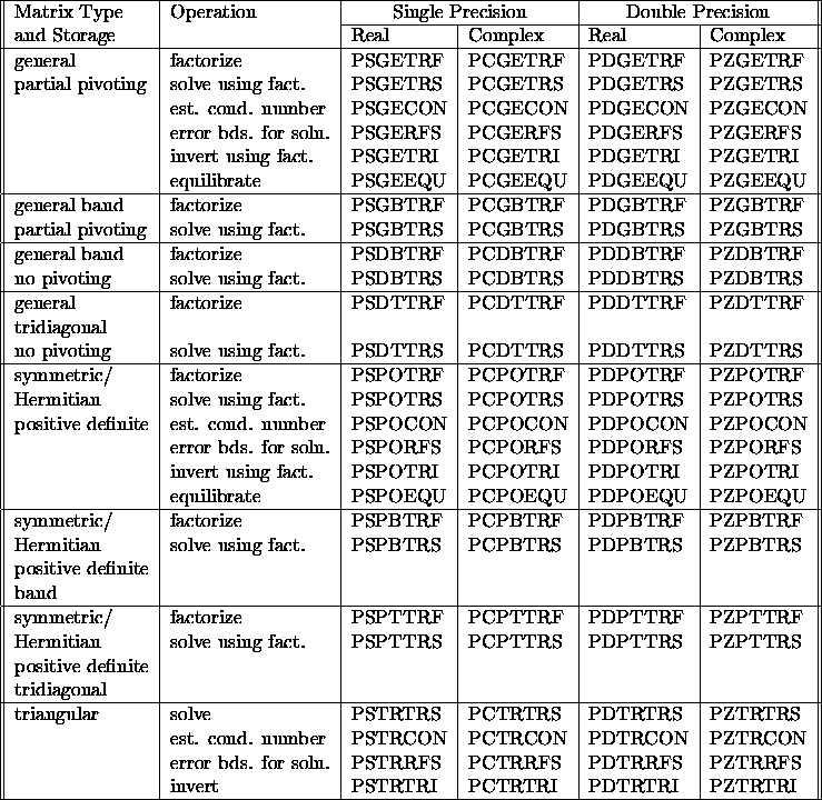
Table 3.6: Computational routines for linear equations