


Next: Implicitly Restarted Arnoldi Method
Up: Arnoldi Method Y. Saad
Previous: Explicit Restarts
Contents
Index
Deflation
We now consider the following implementation which incorporates a
deflation process. So far we have described algorithms that compute
only one eigenpair. In case several eigenpairs are sought,
there are two possible options.
The first is to take  to be a linear combination of the
approximate eigenvectors when we restart. For example, if we need to
compute the
to be a linear combination of the
approximate eigenvectors when we restart. For example, if we need to
compute the  rightmost eigenvectors, we may take
where the eigenvalues are numbered in decreasing order of their real
parts. The vector is then obtained from normalizing  . The simplest choice for the coefficients
  is to take
 . There are several drawbacks to this approach,
the most important of which being that there is no easy way of
choosing the coefficients in a systematic manner. The
result is that for hard problems, convergence is difficult to achieve.
. There are several drawbacks to this approach,
the most important of which being that there is no easy way of
choosing the coefficients in a systematic manner. The
result is that for hard problems, convergence is difficult to achieve.
A more reliable alternative is to compute one eigenpair at a time and
use deflation. The matrix  can be deflated explicitly by
constructing progressively the first
can be deflated explicitly by
constructing progressively the first  Schur vectors. If a previous
orthogonal basis
Schur vectors. If a previous
orthogonal basis
![$U_{k-1} = [u_1,\ldots,u_{k-1}]$](img1925.png) of the invariant
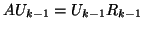
subspace has already been computed, then to compute the eigenvalue
of the invariant
subspace has already been computed, then to compute the eigenvalue
 , we can work with the matrix
in which
 is a
diagonal matrix of shifts. The eigenvalues of
is a
diagonal matrix of shifts. The eigenvalues of  consist of two groups.
Those eigenvalues associated with the Schur vectors
consist of two groups.
Those eigenvalues associated with the Schur vectors
 will be shifted to
 and the others remain unchanged.
If the eigenvalues with largest real parts are sought, then
the shifts are selected so that
and the others remain unchanged.
If the eigenvalues with largest real parts are sought, then
the shifts are selected so that  becomes the next eigenvalue
with largest real part of . It is also possible to
deflate by simply projecting out the components
associated with the invariant subspace spanned by
becomes the next eigenvalue
with largest real part of . It is also possible to
deflate by simply projecting out the components
associated with the invariant subspace spanned by  ;
this would lead to operating with the matrix
;
this would lead to operating with the matrix
Note that if
 is the partial
Schur decomposition associated with the first
is the partial
Schur decomposition associated with the first  Ritz values, then
 .
Those eigenvalues associated with the Schur vectors
will now all be moved to zero.
.
Those eigenvalues associated with the Schur vectors
will now all be moved to zero.
A better implementation of deflation, which
fits in well with the Arnoldi procedure, is
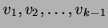
to work with a single basis
 whose first vectors
are the Schur vectors that have already converged. Suppose that
such vectors have converged and call them
whose first vectors
are the Schur vectors that have already converged. Suppose that
such vectors have converged and call them
 . Then we start by choosing a vector
  which is
orthogonal to
which is
orthogonal to
 and of norm 1. Next we perform
 steps of an Arnoldi procedure in which orthogonality of the vector
 against all previous
  's, including
is
enforced. This generates an orthogonal basis of the subspace
's, including
is
enforced. This generates an orthogonal basis of the subspace
 |
(125) |
Thus, the dimension of this modified Krylov subspace is constant and
equal to  in general. A sketch of this implicit deflation procedure
combined with the Arnoldi method appears in the following.
in general. A sketch of this implicit deflation procedure
combined with the Arnoldi method appears in the following.
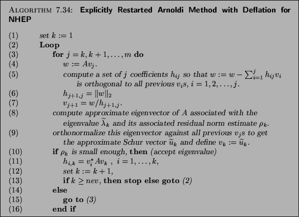
Note that in the Loop, the Schur vectors associated with the
eigenvalues
 will not be touched in subsequent
steps. They are sometimes referred to as ``locked vectors.''
Similarly, the
corresponding upper triangular matrix corresponding to these vectors is
also locked.
will not be touched in subsequent
steps. They are sometimes referred to as ``locked vectors.''
Similarly, the
corresponding upper triangular matrix corresponding to these vectors is
also locked.
When a new Schur vector converges, step (10) computes the th
column of  associated with this new basis vector. In the
subsequent steps, the approximate eigenvalues are the eigenvalues of
the
associated with this new basis vector. In the
subsequent steps, the approximate eigenvalues are the eigenvalues of
the  Hessenberg matrix
  defined in the algorithm
and whose
defined in the algorithm
and whose  principal submatrix is upper triangular.
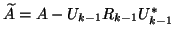
For example, when
principal submatrix is upper triangular.
For example, when  and after the second Schur vector,
  , has
converged, the matrix will have the form
, has
converged, the matrix will have the form
![\begin{displaymath}
H_m ~ = ~
\left[ \begin{array}{cccccc}
* & * & * & * & * &...
... & & & * & * & * \\
& & & & * & * \\
\end{array} \right].
\end{displaymath}](img1945.png) |
(126) |
In the subsequent steps, only the eigenvalues not associated with the
 upper triangular matrix need to be considered.
It can be shown that, in exact arithmetic, the
 Hessenberg matrix in the lower
  block is the same
matrix that would be obtained from an Arnoldi run applied to the
matrix
block is the same
matrix that would be obtained from an Arnoldi run applied to the
matrix
Thus, we are implicitly projecting out the invariant subspace
already computed from the range of .
Next: Implicitly Restarted Arnoldi Method
Up: Arnoldi Method Y. Saad
Previous: Explicit Restarts
Contents
Index
Susan Blackford
2000-11-20

![\begin{displaymath}
\underbrace{\left[v_1, v_2, \ldots, v_{k-1}\right.}_{Locked},
\underbrace{\left. v_k, v_{k+1}, \ldots v_m \right] }_{Active}
\end{displaymath}](img1942.png)