 Incomplete Factorization
Incomplete factorizations with several levels of fill allowed are more
accurate than the  -
- factorization described above. On the
other hand, they require more storage, and are considerably harder to
implement (much of this section is based on algorithms for a full
factorization of a sparse matrix as found in Duff, Erisman and
Reid [80]).
factorization described above. On the
other hand, they require more storage, and are considerably harder to
implement (much of this section is based on algorithms for a full
factorization of a sparse matrix as found in Duff, Erisman and
Reid [80]).
As a preliminary, we need an algorithm for adding two vectors
 and
and  , both stored in sparse storage. Let lx be the number
of nonzero components in , let be stored in x, and let
xind be an integer array such that
, both stored in sparse storage. Let lx be the number
of nonzero components in , let be stored in x, and let
xind be an integer array such that

Similarly, is stored as ly, y, yind.
We now add  by first copying y into
a full vector w then adding w to x. The total number
of operations will be
by first copying y into
a full vector w then adding w to x. The total number
of operations will be 
![]() :
:
% copy y into w
for i=1,ly
   w( yind(i) ) = y(i)
% add w to x wherever x is already nonzero
for i=1,lx
   if w( xind(i) ) <> 0
      x(i) = x(i) + w( xind(i) )
   w( xind(i) ) = 0
% add w to x by creating new components
% wherever x is still zero
for i=1,ly
   if w( yind(i) ) <> 0 then
      lx = lx+1
      xind(lx) = yind(i)
      x(lx) = w( yind(i) )
   endif
In order to add a sequence of vectors
 , we add the
 vectors into
  before executing
the writes into .
A different implementation would be possible, where is allocated
as a sparse vector and its sparsity pattern is constructed during the
additions. We will not discuss this possibility any further.
before executing
the writes into .
A different implementation would be possible, where is allocated
as a sparse vector and its sparsity pattern is constructed during the
additions. We will not discuss this possibility any further.
For a slight refinement of the above algorithm, we will add levels to the nonzero components: we assume integer vectors xlev and ylev of length lx and ly respectively, and a full length level vector wlev corresponding to w. The addition algorithm then becomes:
% copy y into w
for i=1,ly
   w( yind(i) )    = y(i)
   wlev( yind(i) ) = ylev(i)
% add w to x wherever x is already nonzero;
% don't change the levels
for i=1,lx
   if w( xind(i) ) <> 0
      x(i) = x(i) + w( xind(i) )
   w( xind(i) ) = 0
% add w to x by creating new components
% wherever x is still zero;
% carry over levels
for i=1,ly
   if w( yind(i) ) <> 0 then
      lx = lx+1
      x(lx)    = w( yind(i) )
      xind(lx) = yind(i)
      xlev(lx) = wlev( yind(i) )
   endif
We can now describe the factorization. The algorithm starts
out with the matrix A, and gradually builds up
a factorization M of the form 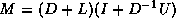 , where
  ,
,
 , and
, and  are stored in the lower triangle, diagonal and
upper triangle of the array M respectively. The particular form
of the factorization is chosen to minimize the number of times that
the full vector w is copied back to sparse form.
are stored in the lower triangle, diagonal and
upper triangle of the array M respectively. The particular form
of the factorization is chosen to minimize the number of times that
the full vector w is copied back to sparse form.
Specifically, we use a sparse form of the following factorization scheme:
for k=1,n
   for j=1,k-1
      for i=j+1,n
         a(k,i) = a(k,i) - a(k,j)*a(j,i)
   for j=k+1,n
      a(k,j) = a(k,j)/a(k,k)
This is a row-oriented version of the traditional `left-looking'
factorization algorithm.
We will describe an incomplete factorization that controls fill-in
through levels (see equation (![]() )). Alternatively we
could use a drop tolerance (section
)). Alternatively we
could use a drop tolerance (section ![]() ), but this is less
attractive from a point of implementation. With fill levels we can
perform the factorization symbolically at first, determining storage
demands and reusing this information through a number of linear
systems of the same sparsity structure. Such preprocessing and reuse
of information is not possible with fill controlled by a drop
tolerance criterion.
), but this is less
attractive from a point of implementation. With fill levels we can
perform the factorization symbolically at first, determining storage
demands and reusing this information through a number of linear
systems of the same sparsity structure. Such preprocessing and reuse
of information is not possible with fill controlled by a drop
tolerance criterion.
The matrix arrays A and M are assumed to be in compressed row storage, with no particular ordering of the elements inside each row, but arrays adiag and mdiag point to the locations of the diagonal elements.
for row=1,n
%  go through elements A(row,col) with col<row
   COPY ROW row OF A() INTO DENSE VECTOR w
   for col=aptr(row),aptr(row+1)-1
      if aind(col) < row then
         acol = aind(col)
         MULTIPLY ROW acol OF M() BY A(col)
         SUBTRACT THE RESULT FROM w
         ALLOWING FILL-IN UP TO LEVEL k
      endif
      INSERT w IN ROW row OF M()
% invert the pivot
   M(mdiag(row)) = 1/M(mdiag(row))
% normalize the row of U
   for col=mptr(row),mptr(row+1)-1
      if mind(col) > row
         M(col) = M(col) * M(mdiag(row))
The structure of a particular sparse matrix is likely to apply to a sequence of problems, for instance on different time-steps, or during a Newton iteration. Thus it may pay off to perform the above incomplete factorization first symbolically to determine the amount and location of fill-in and use this structure for the numerically different but structurally identical matrices. In this case, the array for the numerical values can be used to store the levels during the symbolic factorization phase.