PERFORM - A Fast Simulator For Estimating Program
Execution Time
Alistair Dunlop
and Tony Hey
Department Electronics
and Computer Science
University of Southampton
Southampton, SO17 1BJ, U.K.
November 1997
Keywords - performance estimation, execution-driven
simulation, program slicing, cache memory simulation, memory hierarchy,
automatic program parallelisation
Abstract
This paper describes a performance estimating system developed at
the University of Southampton for estimating the execution time of SPMD
Fortran programs on distributed memory parallel systems. The system called
PERFORM, (Performance EstimatoR For RISC Microprocessors), is an implementation
of a new performance estimating technique based on the concept of execution-driven
simulation. Whereas straightforward execution-driven simulation is slow,
memory intensive and machine specific, our development of this technique
has avoided these traditional problems associated with simulation methods.
Specifically, our development of this method uses a feedback loop to reduce
the amount of code executed during the simulation, while code sections
that do not alter the control flow of the program are removed from the
simulation code. Variables used in removed code sections are also removed
from the simulation code, significantly reducing the memory requirements.
This method is also architecturally independent, in that the properties
and performance characteristics of the target platform can be specified
in a machine description file. Our results show that PERFORM is a substantial
improvement over existing performance estimating methods and that this
tool could be used by programmers for code analysis, or for incorporation
into an automatic/semi-automatic parallel compilation system. PERFORM is
available with either a text-based interface or X-Windows/Motif GUI.
1 The Need For Performance Prediction
Automatic program parallelisation is the main motivating factor driving
research to develop an accurate method for estimating program execution
time. The Achilles heel of parallel computing is the need for users to
develop specialised parallel programs to harness the available computing
power. Although progress has been made in the past few years to simplify
the development of parallel programs, it is still a laborious and time
consuming task when compared to the development of sequential programs.
Accordingly, the parallel software base is almost insignificant when compared
with that available for uni-processor machines. For parallel machines to
become commodity items, it is recognised that they will have to execute
sequential programs directly and efficiently. To this end, much current
research in parallel computing is directed at automatic program parallelisation
([8], [2], [10], [13]). Although there are many research issues still to
be solved by these systems, an issue common to all of them is the need
to identify candidate parallelisation strategies and subsequently determine
the strategy with the best performance. A method is therefore needed to
quantify the difference in execution time between different parallelisation
strategies at compile time. These strategies may differ in both data layout
as well as differing in the sequential code segments. This paper
describes a system developed for this task at the University of Southampton.
2 Methods and Problems of Performance Prediction
The best known performance estimating method is the statement counting
approach popularised by Balasundaram et al [1]. The general hypothesis
of this approach is that the execution time of a program can be determined
by the number and type of operations in the source code, without considering
of the order or the context of these operations. Estimating the execution
time of a program using this method consists of three steps:
-
Determine the execution time of each operation on the target machine. This
can be done a-priori and need only be done once for each target machine,
operating system and compiler tuple.
-
Determine the number and type of operations in the program.
-
Compute the expected execution time of the program on the required target
machine by summing the benchmarked execution times of each operation
in the program.
Implementations of this method differ in their definitions of the ``operations''
and the manner in which the number and type of operations in the target
program is determined. In general, however, the ``operations'' are all
language statements that cannot be reduced to simpler statements, while
the number and type of operations in the input program is determined using
static code analysis and, in some cases, profiling. Irrespective of the
implementation method, results from this approach have shown the method
to be largely unreliable for estimating processor execution time of current
commodity microprocessors. Although some published results show good accuracy
using this method [9] (within 10% of actual execution times), other published
results show that performance estimates can be up to an order of magnitude
different from the benchmarked execution times ([5], [11]). This discrepancy
in results is attributed to both the target hardware and the program code
under consideration [3]. As an example of the unreliability of this method
consider the benchmark code fragment given in figure 1. The predicted and
benchmark results for three different machines are given in figure 2. If
the array f is defined as f(i) = i, the estimated execution time
is within 25% of the actual execution time on machines. However, if the
array f , contains values defined as f(i) = random(1; iterations),
the predicted execution time differs by as much as 5 times the benchmarked
result.
CALL timer(starttime)
DO i=1,iterations
a(f(i)) = b(f(i)) + c(f(i)) + d(f(i))
ENDDO
CALL timer(endtime)
Figure 1: Benchmark to determine the effect of data locality
A further limitation of the statement counting method is that it is unsuitable
for estimating the execution time of optimised programs. Compilers perform
optimisations on statements by having knowledge of the surrounding statements.
In contrast, the statement counting method treats all statements as separate
atomic entities.
Given the importance of data locality in current microprocessor architectures,
performance estimating methods are being developed which attempt to quantify
the amount of time spent moving data within the memory hierarchy. Fahringer
[4] developed a method of statically estimating the number of times a cache
line would have to be replaced in a single-level, direct-mapped, cache
for a given loop. Although this gave some indication of performance, the
approximations were gross, and were unsuitable for converting to execution
time. A more reliable method for computing the number of cache capacity
and conflict misses was developed by Teman et al [12]. This method
is, however, restricted to single-level, direct-mapped caches and has not
been implemented in an automatic tool.
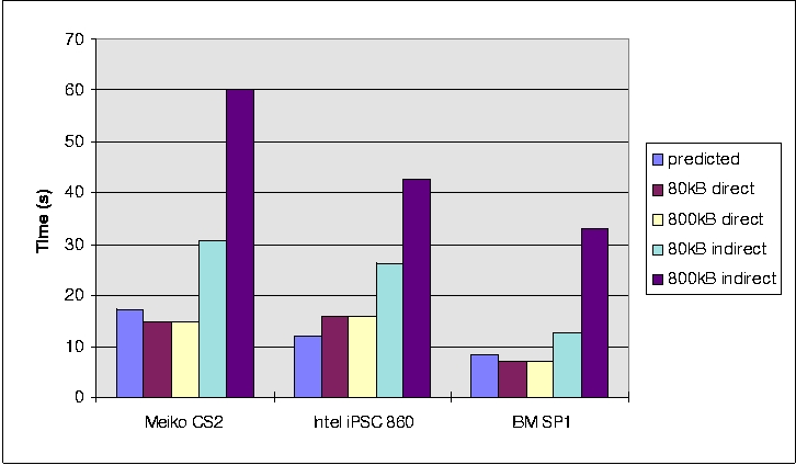 Figure 2: Estimated vs Actual execution times for direct
and indirect addressing on a Meiko CS2, Intel iPSC 860 and IBM SP1
Figure 2: Estimated vs Actual execution times for direct
and indirect addressing on a Meiko CS2, Intel iPSC 860 and IBM SP1
3 The Simulation Solution and PERFORM
Program simulation is an alternative method for predicting program execution
time, but has been generally dismissed on the grounds of being too machine
specific, extremely slow and memory intensive. This is certainly a relevant
argument against using instruction-level simulation and trace-driven
simulation. The most recent form of simulation, execution-driven
simulation, lessens these problems by interleaving the execution of the
input program and the simulation of the architecture. A preprocessor parses
either the assembly language or source code of the program requiring simulation.
This code is modified to extract information during program execution;
hence the term execution-driven simulation. The main advantage of this
form of simulation is that event generation and simulation are coupled
so that feedback can occur. This feedback can be used to alter the ordering,
timing and number of subsequently generated events.
PERFORM, is a performance estimating system we have developed based
on the principle of execution-driven simulation, but avoiding the traditional
simulation problems of generality, speed and memory use. The manner in
which this has been done is outlined below:
-
Improved generality through source code analysis and augmentation.
Our execution-driven simulation method is not machine specific as all code
analysis and augmentation is done at the source code level. Platform specific
features are accounted for during simulation. The gains in generality do
have some impact on the accuracy of the system as the code analyser and
augmenter have to approximate the operations that would be executed on
the target machine.
-
Fast execution-driven simulation. The time to obtain a performance
estimate using our method is substantially lower than that of conventional
execution-driven simulation techniques. This is due to two modifications
that have been made based on the premise that accurate performance estimates
are the only requirement of the system. First, only operations that modify
the system state and therefore affect the execution time of later operations
are simulated. Operations such as ``load'' and ``store'', which take
a variable amount of time to complete depending on the state of the memory
hierarchy are simulated, while arithmetic operations which have constant
execution times are not. The second and most significant way in which
we reduce the execution time of our method is by using a feedback loop
from the simulator engine to the source code. This feedback loop can curtail
the execution of loops in the source code if sufficient information has
been obtained on previous loop iterations to accurately predict the simulated
execution time at the end of the loop.
-
Minimal memory Requirements. One of the main problems with execution-driven
simulation methods is that the executed program requires more memory than
the original input program. Our method reduces the amount of memory
required by the simulation substantially using a technique known as
``program slicing'' [14]. The original input program is first transformed
into a ``sliced'' program in which all variables and data that do not influence
control flow are removed. References to these variables in the program
are also removed. By combining the techniques of program slicing, feedback
loops, limited simulation and source level analysis into execution-driven
simulation, we have developed a method of performance estimation that avoids
the problems commonly associated with simulation, yet retains much of the
accuracy of full simulation. The stages associated with producing the executable
simulation are shown in figure 3.
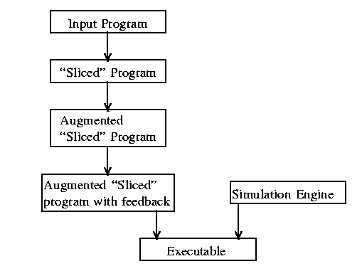 Figure 3: Stages in constructing the fast simulation method
Obtaining a performance estimate using this method can be seen as a
two stage process of analysis and augmentation, followed by execution.
The analysis phase consists of program slicing, while the annotation phase
consists of annotating the sliced code with simulator calls, and inserting
the feedback loop mechanism.
4 Program Slicing within PERFORM
A program slice is a fragment of a program in which some statements are
omitted that are unnecessary to understand a certain property of the program.
For example, if someone is only interested in how the value of AR2 is
computed in the program shown in figure 4, they only need consider the
program slice given in figure 5.
The form of slicing shown in figure 5 is termed an executable program
slice. Our work uses this concept applied to the area of program simulation.
As we are simulating the movement of data within the memory hierarchy the
program slice we generate must maintain sufficient information from the
input program to resolve all data addresses and maintain the order in which
data is accessed. Computation that does not affect the order in which data
is accessed can be removed. The executable program slice must therefore
have the following properties:
-
Control flow must be identical to the input code, and hence all operations
that determine control flow must be included in the sliced program.
-
All operations used to compute array indices must be included in the sliced
program.
SUBROUTINE TEST (N1,AI1,N2,AR1,AR2)
  W = 0.0
  DO I = 1,N1
    W = W + AI1
  ENDDO
  V = 0.0
  DO I = 1,N2
    V = V + I*AI1 + N2
  ENDDO
  AR1 = W
  AR2 = V*2
END
Figure 4: Original program
SUBROUTINE TEST (AI1,N2,AR2)
  V = 0.0
  DO I = 1,N2
    V = V + I*AI1 + N2
  ENDDO
  AR2 = V*2
END
Figure 5: Program in figure 4, sliced on variable AR2
As an example, consider the code fragment given in figure 6. The control
variables are identified in the do loops in program lines 3 and 4, and
are i; N; j. The array index variables occur in line 6 and are i; index;
j. Slicing this program on the union of these variables will result in
the program given in figure 7.
N = 100
index = 0
do i = 1, N
  do j = i-1, i+1, 3
    index = index + 1
    B(i) = B(i) + A(index)*X(j)
  enddo
enddo
Figure 6: Fortran program to calculate B of AX=B
for tridiagonal matrix A
N = 100
index = 0
do i = 1, N
  do j = i-1, i+1, 3
    index = index + 1
  enddo
enddo
Figure 7: Code in figure 6 sliced on variables i; N; j; index
Determining statement minimal program slices is an expensive operation,
requiring at worst n passes for a program with n assignment statements
[6]. Although this solves the general case, it is computationally too expensive
to be used in conjunction with simulation for performance estimation. Accordingly,
we have developed a simpler method that creates a ``restricted'' executable-program
slice in a single pass. This method has been implemented in the PERFORM
system. The difference between our method and general, or full program
slicing, is that in full program slicing, expressions containing control
variables and array index variables would be evaluated as far back as necessary.
That is, if a control variable was a function of non-control and/or non-array
index variables, the program slice would also include assignments to these
variables. Furthermore, if these variables were in turn functions of other
non-control and non-array index variables, assignments to these variables
would be included in the program slice. This process would continue until
all references are resolved; hence requiring up to n passes for a program
with n assignment statements. In contrast our 1-level method excludes this
recursive process, and only statements that are direct assignments to control
and array index variables are included in the program slice. The benefit
of this process is that a program slice can be constructed in a single
source code parse, at the cost of some loss of generality. That is, some
programs may require the user to supply values to some variables that are
not computed as a result of the 1-level program slicing method.
One of the problems with general program slicing is that it may in some
situations, be equivalent to reproducing the entire program. Single-level
program slicing is sufficient to accommodate many applications and provides
three distinct benefits. First, the time required to generate the slice
is less than that required if full program slicing is performed. Second,
by excluding many operations from the simulation control flow, execution
time of the simulation program is improved. Third, and most important,
single-level program slicing will, in most instances, result in a significant
decrease in the amount of memory required when compared with the original
Fortran code. This occurs as only the control variables and array index
variables are defined in the sliced program. Hence, for the program in
figure 6, data space is only reserved for the variables i, j, N and index.
Data space is not required for the arrays B, A, and X. In many applications
this results in the data requirements of the simulation code being only
a few bytes.
5 Simulator Calls in PERFORM
Once the program slice has been created, it is augmented with calls to
the simulator. As the simulation library computes the execution time of
the program, the simulator needs to be notified of all operations that
would occur in the input program. These operations fall into the four areas
of memory access, computation, message passing and subprogram calls. In
the ideal case we would like to generate the same calls to the simulator
that would be executed if the input program was compiled for each target
architecture. Although this would provide the greatest level of confidence
in the simulation results, this would require specific code to be written
for each target architecture, and would be equivalent to second guessing
compiler behaviour. This is not practical. Instead we augment sliced programs
with simulator calls that are the same for all target architectures. In
particular, all operations in the input Fortran program are translated
into a sequence of simulator calls using a stack-based model of computation.
It is the task of the simulation engine to account for architectural differences
at run time.
For example, consider the assignment statement y = sqrt(b2
-4ac) This is translated onto the operation sequence given in figure
8. All symbolic names are bound to specific memory locations at a later
phase.
|
Fortran Input
|
Generated Simlation Operations
|
y=sqrt(b**2 - 4ac)
|
LDREAL(b);
LDREAL(b);
REALOP('*');
LITINTLD(4);
LDREAL(a);
REALOP('*');
LDREAL(c);
REALOP('*');
REALOP('-');
intrinsic_function("sqrt", realtype);
STREAL(y);
|
Figure 8: Translation of y
= sqrt(b2 - 4ac)into simulation instructions
Fortran. That is, the rightmost parameter is the most significant.
Hence, for an array declared a(d0 ; d1 ; d2
) and used in an expression as
(a0 ; a1 ; a2 ), the memory address
accessed is calculated by the expression StartAddress(a) +
(a0 - 1) + (a1 - 1)d0 + (a2
-1 )d0d1.
In all cases the sliced program is augmented with the simulator calls
at the point where the Fortran statement occurs. If the Fortran statement
has been removed from the sliced program, the simulator calls are inserted
at the point where the statement was removed. Additionally, simulator calls
are inserted into the sliced program to represent the computational overhead
associated with control structures such as do
loops and if constructs.
6 Modifying the Execution Path Using Feedback Control
The code augmentation stage described above is sufficient to produce a
complete execution-driven simulation when linked with the simulation library.
The resulting simulation program will, in most cases, take significantly
less memory than the input program, but will take longer to execute as
a result of the added simulator calls. The final part in generating the
execution-driven simulation is to modify the annotated
program slice to restrict the amount of code executed, thereby reducing
the execution time. The simulation execution time is proportional to the
number of instructions simulated. As the majority of operations are confined
to do loops, we reduce the execution time by restricting
the simulation of do loops. This is done by inserting additional code at
the start and end of each do loop construct. The code generated for an
empty loop with a range from 1 to n is shown in figure 9. The call inserted
at the start of the loop, StartTracking(loopiters),
tells the simulator that a new loop of size loopiters
is starting. The call inserted at the end of the loop, CanProjectLoop
is a function call returning either true or false, depending on
whether sufficient information has been gathered to estimate the execution
time at the end of the loop with sufficient accuracy. If this returns true,
any remaining loop iterations are abandoned and the simulator modifies
its state to the projected state at the end of the loop. Execution of the
loop is terminated if successive least-squares approximations to the execution
time at the end of the loop converge.
|
Fortran Input
|
Generated Simulation Operations
|
do i = 1, n LITINTLD(1);
|
STINT(i);
LDINT(n);
LDINT(i);
INTOP('-');
STINT(TEMP 0);
BRCOND ('!=');
StartTracking (int(((n)-(1)+(1))/1));
for (TEMP 0=0; TEMP 0!int(((n)-(1)+(1))/1); TEMP 0++) {
   i=1+(TEMP 0)*(1);
   LDINT(i);
   LITINTLD(1);
   INTOP('+');
   STINT(i);
|
enddo
|
LDINT(TEMP 0);
LITINTLD(1);
INTOP('-');
STINT(TEMP 0);
BRCOND ('?');
if (CanProjectLoop()) break;
} |
Figure 9: Translation of a empty loop into simulation
instructions with calls to reduce simulation
7 Calculating the Execution Time in PERFORM
Before the execution-driven simulation can run, it may be necessary for
the user to provide additional information that could not be obtained using
the single-level code analysis technique. This information may be in the
form of scalars, vectors, or probability values. Scalar values are usually
required to facilitate evaluation of loop variables and define array sizes
in subroutines. Values for entire arrays (vectors) are only needed in a
few situations where the array values are used to access elements of another
array (indirect addressing), and the array values are not computed in the
program using single-level program slicing. Finally, the user may be required
to provide probability values for if statements, if the logical
condition cannot be evaluated completely using the existing sliced variables.
Once all data has been entered by the user, including the required target
machine, the generated code is compiled and linked with the simulation
library. Peformance and architecture details of the target machine are
specified in a separate architecture specification file. Full details of
this file can be found in [3].
On executing the execution-driven simulation, the simulator creates
an internal representation of the register sets and cache memories of the
target hardware as specified in the architecture description file. All
load and store operations modify the state of this memory hierarchy model,
and the time to complete each operation is recorded. Unlike load and store
operations, which have varying execution times, the time
required to complete arithmetic operations and most function calls
is largely constant. Accordingly, these are defined in terms of clock cycles
in the architecture specification file. In situations where the execution
time of arithmetic operations and functions is argument dependent, maximum
and minimum times can be used to define the performance in the architecture
specification file. As the simulator knows nothing about the actual argument
values of these operations, the maximum and minimum times are used to predict
an execution time bound. Message passing operations are treated in a similar
way to function calls. That is, they do not modify the state of the simulator,
and the execution time for an operation is determined from previously benchmarked
operations. In particular, message passing time is estimated using the
benchmarked values of n 1/2 and rinf for the target machine.
This has been shown to be a sufficiently accurate model for the
current generation of high-performance processor interconnects [3].
8 Applicability of the PERFORM System
The PERFORM system has been used in three different types of situations:
-
To predict the execution time of different programs on the same architecture.
Automatic parallelising compilers require an accurate, fast and reliable
solution to this problem. Figure 10 shows the extent to which our method
solves this problem. This figure shows the percent by which the execution
time predicted by PERFORM for the Livermore kernels differs from the benchmarked
results. For comparison, we also show the percent by which the performance
estimates obtained using the statement counting method differ from the
benchmarked results. The estimate errors obtained using PERFORM are within
a much smaller error range, and are on average lower, than those obtained
using statement benchmarking. All predicted execution times were obtained
within a second.
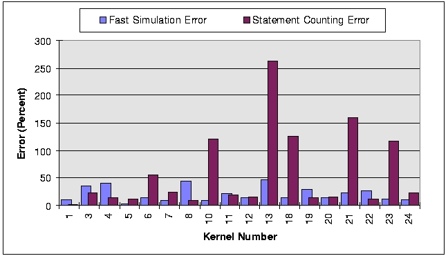 Figure 10: A Comparison of the accuracy of the fast simulation
method versus the statement benchmarking method for the Livermore Kernels
on a SUN SparcStation 1
Figure 10: A Comparison of the accuracy of the fast simulation
method versus the statement benchmarking method for the Livermore Kernels
on a SUN SparcStation 1
-
For analysing code to identify performance anomalies. PERFORM has been
used to perform detailed analysis on benchmark programs to determine
the reason for performance anomalies on different machines and at different
problem sizes.
-
To predict program scalability. PERFORM has also been used to predict changes
in program performance with changes in problem size. Figure 11 is a good
example of this. The predicted performance changes closely match the benchmarked
results throughout the problem sizes. This type of analysis is useful for
identifying optimum problem sizes for a given machine, or for identifying
suitable data partitioning sizes.
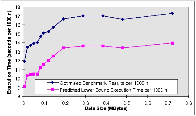 Figure 11: Scalability prediction of Livermore Kernel 18
for small data sizes using fast simulation
Figure 11: Scalability prediction of Livermore Kernel 18
for small data sizes using fast simulation
9 Summary and Conclusion
In this paper we have described the PERFORM system, and shown some performance
predictions obtained
using this method. The key features of this system when compared to
other approaches to performance
estimating are outlined below:
-
Accuracy. We have shown the fast simulation method to be on average
three times more accurate than the statement counting method on the
same architecture.
-
Execution time. The fast simulation method required no more than
2 seconds to estimate the run time of any code tested, even though all
run times were between 10 and 200 seconds on the target hardware. Moreover,
the fast simulation method does not require an initial profile run of the
program like many other approaches.
-
Generality. The fast simulation method is applicable to the vast
majority of scientific Fortran programs. Most scientific Fortran programs
have execution paths that are defined by the problem size, rather than
intermediate computed results. The fast simulation method is directly applicable
to this problem class, but is also applicable to programs whose execution
path is problem dependent, provided that additional static information
concerning the execution path is supplied by the user.
-
Portability. The fast simulation method is highly portable in that
it is neither tied to a specific performance estimating machine, nor is
the intended target hardware fixed or required to be present to obtain
a performance estimate. All target hardware characteristics and performance
information are specified in a machine description file which can easily
and quickly be adapted for different machines.
-
Minimal Memory Requirement. By constructing a program slice from
the input program initially, many data arrays that existed in the input
program are removed from the resulting execution-driven simulation code.
-
Automatic Operation. Obtaining a performance estimate using PERFORM
is a automatic process provided that all loop and branch information
can be deduced from the input program. As a result, this method could be
used by automatic or semi-automatic parallel compilation systems.
In short, PERFORM has many benefits over existing performance estimating
approaches with only a small loss of generality. Current work to extend
this method is addressing some of these shortcommings with the aim of making
this approach fully-automatic for all problem classes.
References
[1] Balasundaram, Vasanth., Fox, Geoffrey., Kennedy, Ken., and Kremer,
Ulrich., A Static Performance Estimator to Guide Data Partitioning Decisions,
ACM Sigplan Notices, 26(7):213-223, 1991.
[2] Chapman, B., Benker, S., Blasko, R., Brezany, P., Egg, M., Fahringer,
T., Gerndt, H.M., Hulman, J., Knaus, B., Kutschera, P., Moritsch, H., Schwald,
A., Sipkova, V., and Zima, H.P., Vienna Fortran Compilation System, Users
Guide, Version 1.0, January 1993.
[3] Dunlop, A.N., Estimating the Execution time of Fortran Programs
on Distributed Memory, Parallel Computers, PhD Thesis, University of Southampton,
1997.
[4] Fahringer, T., Automatic Performance Prediction for Parallel Programs
on Massively Parallel Computers, Phd thesis, University of Vienna, 1993.
[5] Fahringer, Thomas., Evaluation of Benchmark Performance Estimation
for Parallel Fortran Programs on Massively Parallel SIMD and MIMD Computers,
IEEE Proceedings of the 2nd Euromicro Workshop on Parallel and Distributed
Processing, Malaga/Spain, January 1994.
[6] Hausler, P., Denotational program slicing, Proceedings of the 22nd
Hawaii International Conference on System Sciences, vol 2, pp486-494, January
1989.
[7] Hockney, R.W., and Berry, M.W., Public International benchmarks
for Parallel Computers, PARKBENCH Committee report number 1, Scientific
Programming, 3(2):101--146, 1994.
[8] Kennedy, Ken., and Kremer, Ulrich, Automatic Data Layout for High
Performance Fortran, Proceedings of the Workshop on Automatic Data Layout
and Performance Prediction, Rice University, 1995.
[9] MacDonald, N., Predicting the Execution time of Sequential Scientific
Codes, Proceedings International Workshop on Automatic Distributed Memory
Parallelisation, Automatic Data Distribution and Automatic Parallel Performance
Prediction, Saarbrucken, Germany, March 1-3, 1993.
[10] J. H. Merlin, D. B. Carpenter and A. J. G. Hey. SHPF: a Subset
High Performance Fortran compilation system. Fortran Journal, 1996.
[11] Seo, Yoshiki., Kamachi, Tsunehiko., Watanabe, Yukimitsu., Kusano,
Kazuhiro., Suehiro, Kenji., and Shiroto, Yukimasa., Static Performance
Prediction in PCASE: a Programming Environment for Parallel Supercomputers,
NEC Corporation, December 1993.
[12] Temam, Olivier., Fricker, Christine., and Jalby, William, Impact
of Cache Interferences on Usual Numerical Dense Loop Nests, Proceedings
of the IEEE, 81(8):1103-1115, August 1993.
[13] Tseng, C.W., An Optimising Fortran D compiler for MIMD Distributed
Memory Machines, PhD thesis, Rice University, January 1993.
[14] Weiser, Mark., Program Slicing, IEEE Transactions on Software
Engineering, 10(4), July 1984. 10