Footnotes
- ...\title
-
This work was supported in part by
DARPA and ARO under contract number DAAL03-91-C-0047,
the National Science Foundation Science and Technology Center Cooperative
Agreement No. CCR-8809615,
the Applied Mathematical Sciences subprogram of the Office of
Energy Research, U.S. Department of Energy, under Contract
DE-AC05-84OR21400,
and
the Stichting Nationale Computer Faciliteit (NCF) by Grant CRG 92.03.
- ...\author
- Los Alamos National Laboratory,
Los Alamos, NM 87544.
- ...\author
- Department of Computer Science, University of
Tennessee, Knoxville, TN 37996-1301.
- ...\author
- Applied Mathematics Department,
University of California, Los Angeles, CA 90024-1555.
- ...\author
- Computer Science Division and Mathematics
Department, University of California, Berkeley, CA 94720.
- ...\author
- Mathematical Sciences Section,
Oak Ridge National Laboratory, Oak Ridge, TN 37831-6367.
- ...\author
- National Institute of Standards and Technology,
Gaithersburg, MD, 20899
- ...\author
- Department of Mathematics, Utrecht University, Utrecht, the
Netherlands.
- ...
- For a discussion of BLAS as building
blocks, see
[144]
[71]
[70]
[69] and
LAPACK routines
[3]. Also, see
Appendix
 .
.
- ...
- For a more detailed account of the early
history of CG methods, we refer the reader to Golub and
O'Leary
[108] and
Hestenes
[123].
- ...
- Under certain conditions, one can show
that the point Jacobi algorithm is optimal, or close to optimal, in
the sense of reducing the condition number, among all
preconditioners of diagonal form. This was shown by Forsythe and
Strauss for matrices with Property A
[99], and by van der
Sluis
[198] for general sparse matrices. For
extensions to block Jacobi preconditioners, see
Demmel
[66] and Elsner
[95].
- ...
- The SOR and Gauss-Seidel matrices are never used as preconditioners,
for a rather technical reason.
SOR-preconditioning with optimal
 maps the eigenvalues of the
coefficient matrix to a circle in the complex plane;
see Hageman and Young [.3]HaYo:applied. In this case no
polynomial acceleration is possible, i.e., the accelerating polynomial
reduces to the trivial polynomial
maps the eigenvalues of the
coefficient matrix to a circle in the complex plane;
see Hageman and Young [.3]HaYo:applied. In this case no
polynomial acceleration is possible, i.e., the accelerating polynomial
reduces to the trivial polynomial  , and the resulting
method is simply the stationary SOR method.
Recent research by Eiermann and Varga
[84] has shown
that polynomial
acceleration of SOR with suboptimal
will yield no improvement
over simple SOR with optimal
.
, and the resulting
method is simply the stationary SOR method.
Recent research by Eiermann and Varga
[84] has shown
that polynomial
acceleration of SOR with suboptimal
will yield no improvement
over simple SOR with optimal
.
- ...
- To be precise, if we make an incomplete factorization
 , we
refer to positions in
, we
refer to positions in  and
and  when we talk of positions in the
factorization. The matrix
when we talk of positions in the
factorization. The matrix  will have more nonzeros than
and
combined.
will have more nonzeros than
and
combined.
- ...
- The zero refers to the fact that only ``level zero'' fill is
permitted, that is, nonzero elements of the original matrix. Fill
levels are defined by calling an element of level
 if it is
caused by elements at least one of which is of level
if it is
caused by elements at least one of which is of level  .
The first fill level is that caused by the original matrix elements.
.
The first fill level is that caused by the original matrix elements.
- ...
- In graph theoretical terms,
 and
and  -
- coincide if the matrix graph contains no triangles.
- ...
- Writing
 is equally valid, but in practice
harder to implement.
is equally valid, but in practice
harder to implement.
- ...
- On a machine with IEEE Standard
Floating Point Arithmetic,
 in single precision, and
  in double precision.
- ...
- IEEE standard
floating point arithmetic permits computations with
 and
NaN, or Not-a-Number, symbols.
and
NaN, or Not-a-Number, symbols.
- ...
Jack Dongarra
Mon Nov 20 08:52:54 EST 1995
How to Use This Book


Next:
Author's Affiliations
Up:
Templates for the Solution
Previous:
Templates for the Solution
We have divided this book into five main chapters.
Chapter
gives the motivation for this book
and the use of templates.
Chapter
describes
stationary and nonstationary iterative methods. In
this chapter we present both historical development and
state-of-the-art methods for solving some of the most challenging
computational problems facing researchers.
Chapter
focuses on preconditioners. Many
iterative methods depend in part on preconditioners to improve
performance and ensure fast convergence.
Chapter
provides a glimpse of issues related
to the use of iterative methods.
This chapter, like the preceding, is
especially recommended for the experienced user who wishes to have
further guidelines for tailoring a specific code to a particular
machine.
It includes information on complex systems, stopping criteria,
data storage formats, and parallelism.
Chapter
includes overviews of related
topics such as
the close connection between the Lanczos algorithm and the Conjugate
Gradient algorithm, block iterative methods,
red/black orderings,
domain decomposition methods,
multigrid-like methods, and
row-projection schemes.
The Appendices contain information on
how the templates and BLAS software can be
obtained.
A glossary of important terms used in the book is also provided.
The field of iterative methods for solving systems of linear equations
is in constant flux, with new methods and approaches continually being
created, modified, tuned, and some eventually discarded. We expect
the material in this book to undergo changes from time to time as some
of these new approaches mature and become the state-of-the-art.
Therefore, we plan to update the material included in this book
periodically for future editions. We welcome your comments and
criticisms of this work to help us in that updating process. Please
send your comments and questions by email to templates@cs.utk.edu.
List of Symbols
Jack Dongarra
Mon Nov 20 08:52:54 EST 1995
Overview of the Methods
Next:
Stationary Iterative Methods
Up:
Iterative Methods
Previous:
Iterative Methods
Below are short descriptions of each of the methods to be discussed,
along with brief notes on the classification of the methods in terms
of the class of matrices for which they are most appropriate. In
later sections of this chapter more detailed descriptions of these
methods are given.
- Stationary Methods
- Jacobi
.
The Jacobi method is based on solving for every variable locally with
respect to the other variables; one iteration of the method
corresponds to solving for every variable once. The resulting method
is easy to understand and implement, but convergence is slow.
- Gauss-Seidel
.
The Gauss-Seidel method is like the Jacobi method, except that it uses
updated values as soon as they are available.
In general, if the Jacobi method converges, the Gauss-Seidel method
will converge faster than the Jacobi method, though still relatively
slowly.
- SOR
.
Successive Overrelaxation (SOR) can be derived from the Gauss-Seidel
method by introducing an extrapolation parameter
. For the
optimal choice of
, SOR may converge faster than Gauss-Seidel by
an order of magnitude.
- SSOR
.
Symmetric Successive Overrelaxation (SSOR) has no advantage over SOR
as a stand-alone iterative method; however, it is useful as a
preconditioner for nonstationary methods.
- Nonstationary Methods
- Conjugate Gradient (CG
).
The conjugate gradient method derives its name from the fact that it
generates a sequence of conjugate (or orthogonal) vectors. These
vectors are the residuals of the iterates. They are also the
gradients of a quadratic functional, the minimization of which is
equivalent to solving the linear system. CG is an extremely effective
method when the coefficient matrix is symmetric positive definite,
since storage for only a limited number of vectors is required.
- Minimum Residual (MINRES
) and Symmetric LQ
(SYMMLQ
).
These methods are computational alternatives for CG for coefficient
matrices that are symmetric but possibly indefinite. SYMMLQ will
generate the same solution iterates as CG if the coefficient matrix is
symmetric positive definite.
- Conjugate Gradient on the Normal Equations
: CGNE
and CGNR
.
These methods are based on the application of the CG method to one of
two forms of the normal equations
for
 . CGNE solves the system
  for
for  and then
computes the solution
and then
computes the solution  . CGNR solves
  for the solution vector
  where
where  . When the
coefficient matrix
. When the
coefficient matrix  is nonsymmetric and nonsingular, the normal
equations matrices
is nonsymmetric and nonsingular, the normal
equations matrices  and
and  will be symmetric and positive
definite, and hence CG can be applied. The convergence may be slow,
since the spectrum of the normal equations matrices will be less
favorable than the spectrum of
.
will be symmetric and positive
definite, and hence CG can be applied. The convergence may be slow,
since the spectrum of the normal equations matrices will be less
favorable than the spectrum of
.
- Generalized Minimal Residual (GMRES
).
The Generalized Minimal Residual method computes a sequence of
orthogonal vectors (like MINRES), and combines these through a
least-squares solve and update. However, unlike MINRES (and CG) it
requires storing the whole sequence, so that a large amount of storage
is needed. For this reason, restarted versions of this method are
used. In restarted versions, computation and storage costs are
limited by specifying a fixed number of vectors to be generated. This
method is useful for general nonsymmetric matrices.
- BiConjugate Gradient (BiCG
).
The Biconjugate Gradient method generates two CG-like sequences of
vectors, one based on a system with the original coefficient
matrix
, and one on  . Instead of orthogonalizing each
sequence, they are made mutually orthogonal, or
``bi-orthogonal''. This method, like CG, uses
limited storage. It is useful when the matrix is nonsymmetric and
nonsingular; however, convergence may be irregular, and there is a
possibility that the method will break down. BiCG requires a
multiplication with the coefficient matrix and with its transpose at
each iteration.
. Instead of orthogonalizing each
sequence, they are made mutually orthogonal, or
``bi-orthogonal''. This method, like CG, uses
limited storage. It is useful when the matrix is nonsymmetric and
nonsingular; however, convergence may be irregular, and there is a
possibility that the method will break down. BiCG requires a
multiplication with the coefficient matrix and with its transpose at
each iteration.
- Quasi-Minimal Residual (QMR
).
The Quasi-Minimal Residual method applies a least-squares solve and
update to the BiCG residuals, thereby smoothing out the irregular
convergence behavior of BiCG,
which may lead to more reliable approximations.
In full glory, it has a look ahead strategy built in that
avoids the BiCG breakdown.
Even without look ahead,
QMR largely avoids the breakdown that can occur in BiCG.
On the other hand, it does not effect a true minimization of either
the error or the residual, and while it converges smoothly, it often does
not improve on the BiCG in terms of the number of iteration
steps.
- Conjugate Gradient Squared (CGS
).
The Conjugate Gradient Squared method is a variant of BiCG that
applies the updating operations for the
-sequence and the
-sequences both to the same vectors. Ideally, this would double
the convergence rate, but in practice convergence may be much more
irregular than for BiCG,
which may sometimes lead to unreliable results. A practical
advantage is that the method does not need the multiplications with
the transpose of the coefficient matrix.
- Biconjugate Gradient Stabilized (Bi-CGSTAB
).
The Biconjugate Gradient Stabilized method is a variant of BiCG, like
CGS, but using different updates for the
-sequence in order to
obtain smoother convergence than CGS.
- Chebyshev
Iteration.
The Chebyshev Iteration recursively determines polynomials with
coefficients chosen to minimize the norm of the residual in a min-max
sense. The coefficient matrix must be positive definite and knowledge
of the extremal eigenvalues is required. This method has the
advantage of requiring no inner products.
Next:
Stationary Iterative Methods
Up:
Iterative Methods
Previous:
Iterative Methods
Jack Dongarra
Mon Nov 20 08:52:54 EST 1995
Sparse Incomplete Factorizations
Next:
Generating a CRS-based
Up:
Data Structures
Previous:
CDS Matrix-Vector Product
Efficient preconditioners for iterative methods can be found by
performing an incomplete factorization of the coefficient matrix. In
this section, we discuss the incomplete factorization of an  matrix
stored in the CRS format,
and routines to solve a system with such a factorization. At first we
only consider a factorization of the
-
type, that is,
the simplest type of factorization in which no ``fill'' is
allowed, even if the matrix has a nonzero in the fill position (see
section
). Later we will consider factorizations that
allow higher levels of fill. Such factorizations considerably more
complicated to code, but they are essential for complicated
differential equations. The solution routines are applicable in
both cases.
matrix
stored in the CRS format,
and routines to solve a system with such a factorization. At first we
only consider a factorization of the
-
type, that is,
the simplest type of factorization in which no ``fill'' is
allowed, even if the matrix has a nonzero in the fill position (see
section
). Later we will consider factorizations that
allow higher levels of fill. Such factorizations considerably more
complicated to code, but they are essential for complicated
differential equations. The solution routines are applicable in
both cases.
For iterative methods, such as  , that involve a transpose matrix
vector product we need to consider solving a system with the transpose
of as factorization as well.
, that involve a transpose matrix
vector product we need to consider solving a system with the transpose
of as factorization as well.
Jack Dongarra
Mon Nov 20 08:52:54 EST 1995
Generating a CRS-based <IMG ALIGN=BOTTOM SRC="http://www.netlib.org/utk/papers/templates/_22900_tex2html_wrap6389.gif">
-<IMG ALIGN=BOTTOM SRC="http://www.netlib.org/utk/papers/templates/_22900_tex2html_wrap7381.gif">
Incomplete Factorization
Next:
CRS-based Factorization Solve
Up:
Sparse Incomplete Factorizations
Previous:
Sparse Incomplete Factorizations
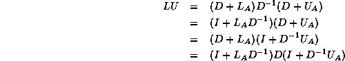
In this subsection we will consider
a matrix split as  in diagonal, lower and upper
triangular part, and an incomplete factorization preconditioner of the form
in diagonal, lower and upper
triangular part, and an incomplete factorization preconditioner of the form
 . In this way, we only need to store a
diagonal matrix
containing the pivots of the factorization.
. In this way, we only need to store a
diagonal matrix
containing the pivots of the factorization.
Hence,it suffices to allocate for the preconditioner only
a pivot array of length  (pivots(1:n)).
In fact, we will store the inverses of the pivots
rather than the pivots themselves. This implies that during
the system solution no divisions have to be performed.
(pivots(1:n)).
In fact, we will store the inverses of the pivots
rather than the pivots themselves. This implies that during
the system solution no divisions have to be performed.
Additionally, we assume that an extra integer array
diag_ptr(1:n)
has been allocated that contains the column (or row) indices of the
diagonal elements in each row, that is, 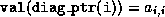 .
.
The factorization begins by copying the matrix diagonal
for i = 1, n
    pivots(i) = val(diag_ptr(i))
end;
Each elimination step starts by inverting the pivot
for i = 1, n
    pivots(i) = 1 / pivots(i)
For all nonzero elements  with
with  , we next check whether
 is a nonzero matrix element, since this is the only element
that can cause fill with
.
is a nonzero matrix element, since this is the only element
that can cause fill with
.
    for j = diag_ptr(i)+1, row_ptr(i+1)-1
        found = FALSE
        for k = row_ptr(col_ind(j)), diag_ptr(col_ind(j))-1
            if(col_ind(k) = i) then
                found = TRUE
                element = val(k)
            endif
        end;
If so, we update  .
.
        if (found = TRUE)
           pivots(col_ind(j)) = pivots(col_ind(j))
                                - element * pivots(i) * val(j)
    end;
end;
Jack Dongarra
Mon Nov 20 08:52:54 EST 1995
CRS-based Factorization Solve
Next:
CRS-based Factorization Transpose
Up:
Sparse Incomplete Factorizations
Previous:
Generating a CRS-based
The system  can be solved in the usual manner by introducing a
temporary vector
can be solved in the usual manner by introducing a
temporary vector  :
:

We have a choice between several equivalent ways of solving the
system:
The first and fourth formulae are not suitable since they require
both multiplication and division with
; the difference between the
second and third is only one of ease of coding. In this section we use
the third formula; in the next section we will use the
second for the transpose system solution.
Both halves of the solution have largely the same structure as the
matrix vector multiplication.
for i = 1, n
    sum =  0
    for j = row_ptr(i), diag_ptr(i)-1
        sum = sum + val(j) * z(col_ind(j))
    end;
    z(i) = pivots(i) * (x(i)-sum)
end;
for i = n, 1, (step -1)
    sum = 0
    for j = diag(i)+1, row_ptr(i+1)-1
        sum = sum + val(j) * y(col_ind(j))
        y(i) = z(i) - pivots(i) * sum
    end;
end;
The temporary vector z can be eliminated by reusing the space
for y; algorithmically, z can even overwrite x, but overwriting input data is in general not recommended
.
Jack Dongarra
Mon Nov 20 08:52:54 EST 1995
CRS-based Factorization Transpose Solve
Next:
Generating a CRS-based
Up:
Sparse Incomplete Factorizations
Previous:
CRS-based Factorization Solve
Solving the transpose system  is slightly more involved. In the usual
formulation we traverse rows when solving a factored system, but here
we can only access columns of the matrices
is slightly more involved. In the usual
formulation we traverse rows when solving a factored system, but here
we can only access columns of the matrices  and
and  (at less
than prohibitive cost). The key idea is to distribute
each newly computed component of a triangular solve immediately over
the remaining right-hand-side.
(at less
than prohibitive cost). The key idea is to distribute
each newly computed component of a triangular solve immediately over
the remaining right-hand-side.
For instance, if we write a lower triangular matrix as
 , then the system
  can be written as
 . Hence, after computing
  we modify
 , and so on. Upper triangular systems are
treated in a similar manner.
With this algorithm we only access columns of the triangular systems.
Solving a transpose system with a matrix stored in CRS format
essentially means that we access rows of
and
.
, and so on. Upper triangular systems are
treated in a similar manner.
With this algorithm we only access columns of the triangular systems.
Solving a transpose system with a matrix stored in CRS format
essentially means that we access rows of
and
.
The algorithm now becomes
for i = 1, n
    x_tmp(i) = x(i)
end;
for i = 1, n
    z(i) = x_tmp(i)
    tmp = pivots(i) * z(i)
    for j = diag_ptr(i)+1, row_ptr(i+1)-1
        x_tmp(col_ind(j)) = x_tmp(col_ind(j)) - tmp * val(j)
    end;
end;
for i = n, 1 (step -1)
    y(i) = pivots(i) * z(i)
    for j = row_ptr(i), diag_ptr(i)-1
        z(col_ind(j)) = z(col_ind(j)) - val(j) * y(i)
    end;
end;
The extra temporary x_tmp is used only for clarity, and can
be overlapped with z. Both x_tmp and z can be
considered to be equivalent to y. Overall, a CRS-based
preconditioner solve uses short vector lengths, indirect addressing,
and has essentially the same memory traffic patterns as that of
the matrix-vector product.
Jack Dongarra
Mon Nov 20 08:52:54 EST 1995
Generating a CRS-based <IMG ALIGN=BOTTOM SRC="http://www.netlib.org/utk/papers/templates/_22900_tex2html_wrap7433.gif">
Incomplete Factorization
Next:
Parallelism
Up:
Sparse Incomplete Factorizations
Previous:
CRS-based Factorization Transpose
Incomplete factorizations with several levels of fill allowed are more
accurate than the
-
factorization described above. On the
other hand, they require more storage, and are considerably harder to
implement (much of this section is based on algorithms for a full
factorization of a sparse matrix as found in Duff, Erisman and
Reid
[80]).
As a preliminary, we need an algorithm for adding two vectors
and
, both stored in sparse storage. Let lx be the number
of nonzero components in
, let
be stored in x, and let
xind be an integer array such that

Similarly,
is stored as ly, y, yind.
We now add 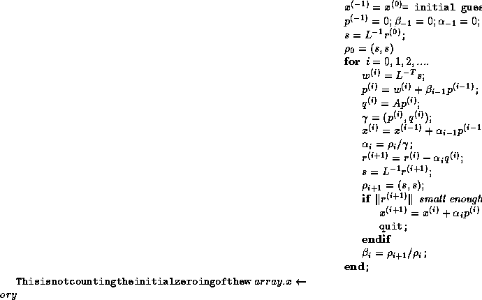 by first copying y into
a full vector w then adding w to x. The total number
of operations will be
by first copying y into
a full vector w then adding w to x. The total number
of operations will be 
 :
:
% copy y into w
for i=1,ly
   w( yind(i) ) = y(i)
% add w to x wherever x is already nonzero
for i=1,lx
   if w( xind(i) ) <> 0
      x(i) = x(i) + w( xind(i) )
   w( xind(i) ) = 0
% add w to x by creating new components
% wherever x is still zero
for i=1,ly
   if w( yind(i) ) <> 0 then
      lx = lx+1
      xind(lx) = yind(i)
      x(lx) = w( yind(i) )
   endif
In order to add a sequence of vectors
 , we add the
 vectors into
  before executing
the writes into
.
A different implementation would be possible, where
is allocated
as a sparse vector and its sparsity pattern is constructed during the
additions. We will not discuss this possibility any further.
before executing
the writes into
.
A different implementation would be possible, where
is allocated
as a sparse vector and its sparsity pattern is constructed during the
additions. We will not discuss this possibility any further.
For a slight refinement of the above algorithm,
we will add levels to the nonzero components:
we assume integer vectors xlev and ylev of length lx
and ly respectively, and a full length level vector wlev
corresponding to w. The addition algorithm then becomes:
% copy y into w
for i=1,ly
   w( yind(i) )    = y(i)
   wlev( yind(i) ) = ylev(i)
% add w to x wherever x is already nonzero;
% don't change the levels
for i=1,lx
   if w( xind(i) ) <> 0
      x(i) = x(i) + w( xind(i) )
   w( xind(i) ) = 0
% add w to x by creating new components
% wherever x is still zero;
% carry over levels
for i=1,ly
   if w( yind(i) ) <> 0 then
      lx = lx+1
      x(lx)    = w( yind(i) )
      xind(lx) = yind(i)
      xlev(lx) = wlev( yind(i) )
   endif
We can now describe the  factorization. The algorithm starts
out with the matrix A, and gradually builds up
a factorization M of the form
factorization. The algorithm starts
out with the matrix A, and gradually builds up
a factorization M of the form  , where
,
, where
,
 , and
, and  are stored in the lower triangle, diagonal and
upper triangle of the array M respectively. The particular form
of the factorization is chosen to minimize the number of times that
the full vector w is copied back to sparse form.
are stored in the lower triangle, diagonal and
upper triangle of the array M respectively. The particular form
of the factorization is chosen to minimize the number of times that
the full vector w is copied back to sparse form.
Specifically, we use a sparse form of the following factorization
scheme:
for k=1,n
   for j=1,k-1
      for i=j+1,n
         a(k,i) = a(k,i) - a(k,j)*a(j,i)
   for j=k+1,n
      a(k,j) = a(k,j)/a(k,k)
This is a row-oriented version of the traditional `left-looking'
factorization algorithm.
We will describe an incomplete factorization that controls fill-in
through levels (see equation (
)). Alternatively we
could use a drop tolerance (section
), but this is less
attractive from a point of implementation. With fill levels we can
perform the factorization symbolically at first, determining storage
demands and reusing this information through a number of linear
systems of the same sparsity structure. Such preprocessing and reuse
of information is not possible with fill controlled by a drop
tolerance criterion.
The matrix
arrays A and M are assumed to be in compressed row
storage, with no particular ordering of the elements inside each row,
but arrays adiag and mdiag point to the locations of the
diagonal elements.
for row=1,n
%  go through elements A(row,col) with col<row
   COPY ROW row OF A() INTO DENSE VECTOR w
   for col=aptr(row),aptr(row+1)-1
      if aind(col) < row then
         acol = aind(col)
         MULTIPLY ROW acol OF M() BY A(col)
         SUBTRACT THE RESULT FROM w
         ALLOWING FILL-IN UP TO LEVEL k
      endif
      INSERT w IN ROW row OF M()
% invert the pivot
   M(mdiag(row)) = 1/M(mdiag(row))
% normalize the row of U
   for col=mptr(row),mptr(row+1)-1
      if mind(col) > row
         M(col) = M(col) * M(mdiag(row))
The structure of a particular sparse matrix is likely to apply to a
sequence of problems, for instance on different time-steps, or during
a Newton iteration. Thus it may pay off to perform the above
incomplete factorization first symbolically to determine the amount
and location of fill-in and use this structure for the numerically
different but structurally identical matrices. In this case, the
array for the numerical values can be used to store the levels during
the symbolic factorization phase.
Next:
Parallelism
Up:
Sparse Incomplete Factorizations
Previous:
CRS-based Factorization Transpose
Jack Dongarra
Mon Nov 20 08:52:54 EST 1995
Parallelism
Next:
Inner products
Up:
Related Issues
Previous:
Generating a CRS-based
Pipelining: See: Vector computer.
Vector computer: Computer that is able to process
consecutive identical operations (typically additions or multiplications)
several times faster than intermixed operations of different types.
Processing identical operations this way is called `pipelining'
the operations.
Shared memory: See: Parallel computer.
Distributed memory: See: Parallel computer.
Message passing: See: Parallel computer.
Parallel computer: Computer with multiple independent
processing units. If the processors have immediate access to the
same memory, the memory is said to be shared; if processors have
private memory that is not immediately visible to other processors,
the memory is said to be distributed. In that case, processors
communicate by message passing.
In this section we discuss aspects of parallelism in the
iterative methods discussed in this book.
Since the iterative methods share most of their computational kernels
we will discuss these independent of the method.
The basic time-consuming kernels of iterative schemes are:
- inner products,
- vector updates,
- matrix-vector products, e.g.,
 (for some methods also
  ),
),
- preconditioner solves.
We will examine each of these in turn. We will conclude this section
by discussing two particular issues, namely computational wavefronts
in the SOR method,
and block operations in the GMRES method.
Jack Dongarra
Mon Nov 20 08:52:54 EST 1995
Inner products
Next:
Overlapping communication and
Up:
Parallelism
Previous:
Parallelism
The computation of an inner product of two vectors
can be easily parallelized; each processor computes the
inner product of corresponding segments of each vector
(local inner products or LIPs).
On distributed-memory machines the LIPs then
have to be sent to other processors
to be combined for the global inner product. This can be done either
with an all-to-all send where every processor performs the summation
of the LIPs, or by a global accumulation in one processor, followed by
a broadcast of the final result.
Clearly, this step requires communication.
For shared-memory machines, the accumulation of LIPs can be
implemented as a critical section where all processors add their local
result in turn to the global result, or as a piece of serial
code, where one processor performs the summations.
Jack Dongarra
Mon Nov 20 08:52:54 EST 1995
Overlapping communication and computation
Next:
Fewer synchronization points
Up:
Inner products
Previous:
Inner products
Clearly, in the usual formulation of conjugate gradient-type methods
the inner products induce a synchronization of the
processors, since they cannot progress until the final result has been
computed:
updating  and
and  can only begin after
completing the inner product for
can only begin after
completing the inner product for  . Since on a
distributed-memory machine communication is needed for the inner product, we
cannot overlap this communication with useful computation.
The same observation applies to updating
. Since on a
distributed-memory machine communication is needed for the inner product, we
cannot overlap this communication with useful computation.
The same observation applies to updating  , which can only begin
after completing the inner product for
, which can only begin
after completing the inner product for  .
.
Figure
shows a variant of CG, in which all
communication time may be overlapped with useful computations. This
is just a reorganized version of the original CG scheme, and is
therefore precisely as stable. Another advantage over other
approaches (see below) is that no additional operations are required.
This rearrangement is based on two tricks. The first is that updating
the iterate is delayed to mask the communication stage of the
 inner product. The second trick relies on splitting the
(symmetric) preconditioner as
inner product. The second trick relies on splitting the
(symmetric) preconditioner as  , so one first computes
 , after which the inner product
 can be computed as
  where
where  . The
computation of
. The
computation of  will then mask the communication stage of the
inner product.
will then mask the communication stage of the
inner product.

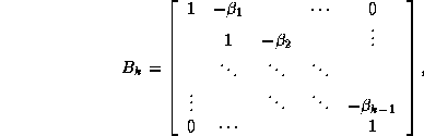
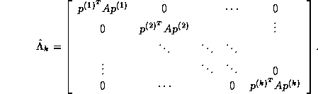
Figure: A rearrangement of Conjugate Gradient for parallelism
Under the assumptions that we have made, CG can be efficiently parallelized
as follows:
- The communication required for the reduction of the inner
product for
 can be overlapped with the update for
  ,
(which could in fact have been done in the previous iteration step).
,
(which could in fact have been done in the previous iteration step).
- The reduction of the inner product for
 can be
overlapped with the remaining part of the preconditioning operation
at the beginning of the next iteration.
can be
overlapped with the remaining part of the preconditioning operation
at the beginning of the next iteration.
- The computation of a segment of
can be followed
immediately by the computation of a segment of
 , and this can
be followed by the computation of a part of the inner product. This
saves on load operations for segments of
and
.
, and this can
be followed by the computation of a part of the inner product. This
saves on load operations for segments of
and
.
For a more detailed discussion see Demmel, Heath and
Van der Vorst
[67]. This algorithm
can be extended trivially to preconditioners of  form, and
nonsymmetric preconditioners in the Biconjugate Gradient Method.
form, and
nonsymmetric preconditioners in the Biconjugate Gradient Method.
Next:
Fewer synchronization points
Up:
Inner products
Previous:
Inner products
Jack Dongarra
Mon Nov 20 08:52:54 EST 1995
Fewer synchronization points
Next:
Vector updates
Up:
Inner products
Previous:
Overlapping communication and
Several authors have found ways to eliminate some of the
synchronization points induced by the
inner products in methods such as CG. One strategy has been to
replace one of the two inner products typically present in conjugate
gradient-like methods by one or two others in such a way that all
inner products can be performed simultaneously. The global
communication can then be packaged. A first such method was proposed
by Saad
[182] with a modification to improve its
stability suggested by Meurant
[156]. Recently, related
methods have been
proposed by Chronopoulos and Gear
[55], D'Azevedo and
Romine
[62], and Eijkhout
[88].
These schemes can also be applied to
nonsymmetric methods such as BiCG. The stability of such methods is
discussed by D'Azevedo, Eijkhout and Romine
[61].
Another approach is to generate a number of
successive Krylov vectors (see §
) and
orthogonalize these as a block (see
Van Rosendale
[210], and Chronopoulos and
Gear
[55]).
Jack Dongarra
Mon Nov 20 08:52:54 EST 1995
Vector updates
Next:
Matrix-vector products
Up:
Parallelism
Previous:
Fewer synchronization points
Vector updates are trivially parallelizable: each processor updates its
own segment.
Jack Dongarra
Mon Nov 20 08:52:54 EST 1995
Stationary Iterative Methods
Next:
The Jacobi Method
Up:
Iterative Methods
Previous:
Overview of the
Iterative methods that can be expressed in the simple form

(where neither  nor
nor  depend upon the iteration count
) are
called stationary iterative methods.
In this section, we present the four main stationary iterative
methods: the Jacobi
method, the Gauss-Seidel
method, the Successive
Overrelaxation
(SOR) method and
the Symmetric Successive Overrelaxation
(SSOR) method.
In each case,
we summarize their convergence behavior and their effectiveness, and
discuss how and when they should be used. Finally,
in §
, we give some historical background and
further notes and references.
depend upon the iteration count
) are
called stationary iterative methods.
In this section, we present the four main stationary iterative
methods: the Jacobi
method, the Gauss-Seidel
method, the Successive
Overrelaxation
(SOR) method and
the Symmetric Successive Overrelaxation
(SSOR) method.
In each case,
we summarize their convergence behavior and their effectiveness, and
discuss how and when they should be used. Finally,
in §
, we give some historical background and
further notes and references.
Jack Dongarra
Mon Nov 20 08:52:54 EST 1995
Matrix-vector products
Next:
Preconditioning
Up:
Parallelism
Previous:
Vector updates
The matrix-vector products are often easily parallelized on shared-memory
machines by splitting the matrix in strips corresponding to the vector
segments. Each processor then computes the matrix-vector product of one
strip.
For distributed-memory machines, there may be a problem if each processor
has only a segment of the vector in its memory. Depending on the bandwidth
of the matrix, we may need communication for other elements of the vector,
which may lead to communication bottlenecks. However, many sparse
matrix problems arise from a network in which only nearby nodes are
connected. For example, matrices stemming
from finite difference or finite element problems typically involve
only local connections: matrix element
is nonzero
only if variables  and
and  are physically close.
In such a case, it seems natural to subdivide the network, or
grid, into suitable blocks and to distribute them over the processors.
When computing
are physically close.
In such a case, it seems natural to subdivide the network, or
grid, into suitable blocks and to distribute them over the processors.
When computing  , each processor requires the values of
  at
some nodes in neighboring blocks. If the number of connections to these
neighboring blocks is small compared to the number of internal nodes,
then the communication time can be overlapped with computational work.
For more detailed discussions on implementation aspects for distributed
memory systems, see De Sturler
[63] and
Pommerell
[175].
at
some nodes in neighboring blocks. If the number of connections to these
neighboring blocks is small compared to the number of internal nodes,
then the communication time can be overlapped with computational work.
For more detailed discussions on implementation aspects for distributed
memory systems, see De Sturler
[63] and
Pommerell
[175].
Jack Dongarra
Mon Nov 20 08:52:54 EST 1995
Preconditioning
Next:
Discovering parallelism in
Up:
Parallelism
Previous:
Matrix-vector products
Preconditioning is often the most problematic part of parallelizing
an iterative method.
We will mention a number of approaches to obtaining parallelism in
preconditioning.
Jack Dongarra
Mon Nov 20 08:52:54 EST 1995
Discovering parallelism in sequential preconditioners.
Next:
More parallel variants
Up:
Preconditioning
Previous:
Preconditioning
Certain preconditioners were not developed with parallelism in mind,
but they can be executed in parallel. Some examples are domain
decomposition methods (see §
), which
provide a high degree of coarse grained parallelism,
and polynomial preconditioners
(see §
), which have the same parallelism as
the matrix-vector product.
Incomplete factorization preconditioners are usually much harder to
parallelize: using wavefronts of independent computations (see for
instance Paolini and Radicati di Brozolo
[170]) a
modest amount of parallelism
can be attained, but the implementation is complicated. For instance,
a central difference discretization on regular grids gives wavefronts
that are hyperplanes
(see Van der Vorst
[205]
[203]).
Jack Dongarra
Mon Nov 20 08:52:54 EST 1995
More parallel variants of sequential preconditioners.
Next:
Fully decoupled preconditioners.
Up:
Preconditioning
Previous:
Discovering parallelism in
Variants of existing sequential incomplete factorization
preconditioners with a higher degree of parallelism have been devised,
though they are perhaps less efficient in purely scalar terms than
their ancestors. Some examples are: reorderings of the
variables (see Duff and Meurant
[79] and
Eijkhout
[85]), expansion of the
factors in a truncated Neumann series (see
Van der Vorst
[201]),
various block factorization methods (see
Axelsson and Eijkhout
[15]
and
Axelsson and Polman
[21]),
and multicolor preconditioners.
Multicolor preconditioners have optimal parallelism among incomplete
factorization methods, since the minimal number of sequential steps
equals the color number of the matrix graphs. For theory and
applications to parallelism
see Jones and Plassman
[128]
[127].
Jack Dongarra
Mon Nov 20 08:52:54 EST 1995
Fully decoupled preconditioners.
Next:
Wavefronts in the
Up:
Preconditioning
Previous:
More parallel variants
If all processors execute their part of the preconditioner solve
without further communication, the overall method is technically a
block Jacobi preconditioner (see §
).
While their parallel execution is very efficient, they
may not be as effective as more complicated, less parallel
preconditioners, since improvement in the number of iterations
may be only modest.
To get a bigger improvement while retaining the efficient parallel
execution,
Radicati di Brozolo and Robert
[178] suggest that one construct
incomplete decompositions on slightly overlapping domains. This requires
communication similar to that for matrix-vector products.
Jack Dongarra
Mon Nov 20 08:52:54 EST 1995
Wavefronts in the Gauss-Seidel and Conjugate Gradient methods
Next:
Blocked operations in
Up:
Parallelism
Previous:
Fully decoupled preconditioners.
At first sight, the Gauss-Seidel method (and the SOR method which has
the same basic structure) seems to be a fully sequential method.
A more careful analysis, however, reveals a high degree of parallelism
if the method is applied to sparse matrices such as those arising from
discretized partial differential equations.
We start by partitioning the unknowns in wavefronts. The first
wavefront contains those unknowns that (in the directed graph of
 ) have no predecessor; subsequent wavefronts are then sets (this
definition is not necessarily unique) of successors of elements of the
previous wavefront(s), such that no successor/predecessor relations hold
among the elements of this set. It is clear that all elements of a
wavefront can be processed simultaneously, so the sequential time of
solving a system with
can be reduced to the number of
wavefronts.
) have no predecessor; subsequent wavefronts are then sets (this
definition is not necessarily unique) of successors of elements of the
previous wavefront(s), such that no successor/predecessor relations hold
among the elements of this set. It is clear that all elements of a
wavefront can be processed simultaneously, so the sequential time of
solving a system with
can be reduced to the number of
wavefronts.
Next, we observe that the unknowns in a wavefront can be computed as
soon as all wavefronts containing its predecessors have been computed.
Thus we can, in the absence of tests for convergence, have components
from several iterations being computed simultaneously.
Adams and Jordan
[2] observe that in this way
the natural ordering of unknowns gives an iterative method that is
mathematically equivalent to a multi-color ordering.
In the multi-color ordering, all wavefronts of the same color are
processed simultaneously. This reduces the number of sequential steps
for solving the Gauss-Seidel matrix to the number of colors, which is
the smallest number  such that wavefront
contains no
elements that are a predecessor of an element in wavefront
such that wavefront
contains no
elements that are a predecessor of an element in wavefront  .
.
As demonstrated by O'Leary
[164], SOR theory still holds
in an approximate sense for multi-colored matrices. The above
observation that the Gauss-Seidel method with the natural ordering is
equivalent to a multicoloring cannot be extended to the SSOR method or
wavefront-based incomplete factorization preconditioners for the
Conjugate Gradient method. In fact, tests by Duff and
Meurant
[79] and
an analysis by Eijkhout
[85] show that multicolor incomplete
factorization preconditioners in general may take a considerably
larger number of iterations to converge than preconditioners based on
the natural ordering. Whether this is offset by the increased
parallelism depends on the application and the computer architecture.
Next:
Blocked operations in
Up:
Parallelism
Previous:
Fully decoupled preconditioners.
Jack Dongarra
Mon Nov 20 08:52:54 EST 1995
Blocked operations in the GMRES method
Next:
Remaining topics
Up:
Parallelism
Previous:
Wavefronts in the
In addition to the usual matrix-vector product, inner products and
vector updates, the preconditioned GMRES method
(see §
) has a kernel where one new vector,
 , is orthogonalized against the previously built
orthogonal set {
, is orthogonalized against the previously built
orthogonal set { ,
,  ,...,
,...,  }.
In our version, this is
done using Level 1 BLAS, which may be quite inefficient. To
incorporate Level 2 BLAS we can apply either Householder
orthogonalization or classical Gram-Schmidt twice (which mitigates
classical Gram-Schmidt's potential instability; see
Saad
[185]). Both
approaches significantly increase the computational work, but using
classical Gram-Schmidt has the advantage that all inner products can
be performed simultaneously; that is, their communication can be
packaged. This may increase the efficiency of the computation
significantly.
}.
In our version, this is
done using Level 1 BLAS, which may be quite inefficient. To
incorporate Level 2 BLAS we can apply either Householder
orthogonalization or classical Gram-Schmidt twice (which mitigates
classical Gram-Schmidt's potential instability; see
Saad
[185]). Both
approaches significantly increase the computational work, but using
classical Gram-Schmidt has the advantage that all inner products can
be performed simultaneously; that is, their communication can be
packaged. This may increase the efficiency of the computation
significantly.
Another way to obtain more parallelism and
data locality is to generate a basis
{
,  , ...,
  } for the Krylov subspace first,
and to orthogonalize this set afterwards; this is called
} for the Krylov subspace first,
and to orthogonalize this set afterwards; this is called
 -step GMRES(
) (see Kim and Chronopoulos
[139]).
(Compare this to the GMRES method in §
, where each
new vector is immediately orthogonalized to all previous vectors.)
This approach does not
increase the computational work and, in contrast to CG, the numerical
instability due to generating a possibly near-dependent set is not
necessarily a drawback.
-step GMRES(
) (see Kim and Chronopoulos
[139]).
(Compare this to the GMRES method in §
, where each
new vector is immediately orthogonalized to all previous vectors.)
This approach does not
increase the computational work and, in contrast to CG, the numerical
instability due to generating a possibly near-dependent set is not
necessarily a drawback.
Jack Dongarra
Mon Nov 20 08:52:54 EST 1995
Remaining topics
Next:
The Lanczos Connection
Up:
Templates for the Solution
Previous:
Blocked operations in
Jack Dongarra
Mon Nov 20 08:52:54 EST 1995
The Lanczos Connection
Next:
Block and -step
Up:
Remaining topics
Previous:
Remaining topics
As discussed by Paige and Saunders in
[168] and by
Golub and Van Loan in
[109], it is straightforward to
derive the conjugate gradient method for solving symmetric positive
definite linear systems from the Lanczos algorithm for solving
symmetric eigensystems and vice versa. As an example, let us consider
how one can derive the Lanczos process for symmetric eigensystems from
the (unpreconditioned) conjugate gradient method.
Suppose we define the  matrix
  by
by

and the  upper bidiagonal matrix
  by
by
where the sequences  and
and  are defined by the standard
conjugate gradient algorithm discussed in §
.
From the equations
are defined by the standard
conjugate gradient algorithm discussed in §
.
From the equations

and  , we have
  , where

Assuming the elements of the sequence  are
-conjugate,
it follows that
are
-conjugate,
it follows that

is a tridiagonal matrix since
Since span{ } =
span{
} =
span{ } and since the elements of
 are mutually orthogonal, it can be shown that the columns of
matrix
are mutually orthogonal, it can be shown that the columns of
matrix  form an orthonormal basis
for the subspace
form an orthonormal basis
for the subspace 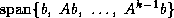 , where
 is a diagonal matrix whose
th diagonal element is
is a diagonal matrix whose
th diagonal element is  . The columns of the matrix
  are the Lanczos vectors (see
Parlett
[171]) whose associated projection of
is
the tridiagonal matrix
are the Lanczos vectors (see
Parlett
[171]) whose associated projection of
is
the tridiagonal matrix

The extremal eigenvalues of  approximate those of the
matrix
. Hence,
the diagonal and subdiagonal elements of
in
(
), which are readily available during iterations of the
conjugate gradient algorithm (§
),
can be used to construct
after
CG iterations. This
allows us to obtain good approximations to the extremal eigenvalues
(and hence the condition number) of the matrix
while we are generating
approximations,
approximate those of the
matrix
. Hence,
the diagonal and subdiagonal elements of
in
(
), which are readily available during iterations of the
conjugate gradient algorithm (§
),
can be used to construct
after
CG iterations. This
allows us to obtain good approximations to the extremal eigenvalues
(and hence the condition number) of the matrix
while we are generating
approximations,  , to the solution of the linear system
.
, to the solution of the linear system
.
For a nonsymmetric matrix
, an equivalent nonsymmetric Lanczos
algorithm (see Lanczos
[142]) would produce a
nonsymmetric matrix
in (
) whose extremal eigenvalues
(which may include complex-conjugate pairs) approximate those of
.
The nonsymmetric Lanczos method is equivalent to the BiCG method
discussed in §
.
Next:
Block and -step
Up:
Remaining topics
Previous:
Remaining topics
Jack Dongarra
Mon Nov 20 08:52:54 EST 1995
Block and <IMG ALIGN=BOTTOM SRC="http://www.netlib.org/utk/papers/templates/_22900_tex2html_wrap7625.gif">
-step Iterative Methods
Next:
Reduced System Preconditioning
Up:
Remaining topics
Previous:
The Lanczos Connection
The methods discussed so far are all subspace methods, that is, in
every iteration they extend the dimension of the subspace generated. In
fact, they generate an orthogonal basis for this subspace, by
orthogonalizing the newly generated vector with respect to the
previous basis vectors.
However, in the case of nonsymmetric coefficient matrices the newly
generated vector may be almost linearly dependent on the existing
basis. To prevent break-down or severe numerical error in such
instances, methods have been proposed that perform a look-ahead step
(see Freund, Gutknecht and
Nachtigal
[101], Parlett, Taylor and
Liu
[172], and Freund and
Nachtigal
[102]).
Several new, unorthogonalized, basis
vectors are generated and are then orthogonalized with
respect to the subspace already generated. Instead of generating a
basis, such a method generates a series of low-dimensional orthogonal
subspaces.
The  -step iterative methods of Chronopoulos and
Gear
[55] use this strategy of generating
unorthogonalized vectors and processing them as a block to reduce
computational overhead and improve processor cache behavior.
-step iterative methods of Chronopoulos and
Gear
[55] use this strategy of generating
unorthogonalized vectors and processing them as a block to reduce
computational overhead and improve processor cache behavior.
If conjugate gradient methods are considered to generate a
factorization of a tridiagonal reduction of the original matrix, then
look-ahead methods generate a block factorization of a block
tridiagonal reduction of the matrix.
A block tridiagonal reduction is also effected by the
Block Lanczos algorithm and the Block Conjugate Gradient
method
(see O'Leary
[163]).
Such methods operate on multiple linear systems with the same
coefficient matrix simultaneously, for instance with multiple right hand
sides, or the same right hand side but with different initial guesses.
Since these block methods use multiple search directions in each step,
their convergence behavior is better than for ordinary methods. In fact,
one can show that the spectrum of the matrix is effectively
reduced by the  smallest eigenvalues, where
  is the block
size.
is the block
size.
Next:
Reduced System Preconditioning
Up:
Remaining topics
Previous:
The Lanczos Connection
Jack Dongarra
Mon Nov 20 08:52:54 EST 1995
The Jacobi Method
Next:
Convergence of the
Up:
Stationary Iterative Methods
Previous:
Stationary Iterative Methods
The Jacobi method is easily derived by examining each of
the
equations in the linear system
in isolation. If in
the
th equation

we solve for the value of  while assuming the other entries
of
remain fixed, we obtain
while assuming the other entries
of
remain fixed, we obtain

This suggests an iterative method defined by

which is the Jacobi method. Note that the order in which the
equations are examined is irrelevant, since the Jacobi method treats
them independently. For this reason, the Jacobi method is also known
as the method of simultaneous displacements, since the updates
could in principle be done simultaneously.
Simultaneous displacements, method of: Jacobi method.
In matrix terms, the definition of the Jacobi method
in (
) can be expressed as

where the matrices
,  and
and  represent the diagonal, the
strictly lower-triangular, and the strictly upper-triangular parts of
,
respectively.
represent the diagonal, the
strictly lower-triangular, and the strictly upper-triangular parts of
,
respectively.
The pseudocode for the Jacobi method is given in Figure
.
Note that an auxiliary storage vector,  is used in the
algorithm. It is not possible to update the vector
in place,
since values from
is used in the
algorithm. It is not possible to update the vector
in place,
since values from  are needed throughout the
computation of
.
are needed throughout the
computation of
.
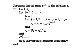
Figure: The Jacobi Method
Jack Dongarra
Mon Nov 20 08:52:54 EST 1995
Reduced System Preconditioning
Next:
Domain Decomposition Methods
Up:
Remaining topics
Previous:
Block and -step
Reduced system: Linear system obtained by eliminating
certain variables from another linear system.
Although the number of variables is smaller
than for the original system, the matrix of a reduced system generally
has more nonzero entries. If the original matrix was symmetric and positive
definite, then the reduced system has a smaller condition number.
As we have seen earlier, a suitable preconditioner for CG is a
matrix
such that the system

requires fewer iterations to solve than  does, and for which
systems
does, and for which
systems  can be solved efficiently. The first property is
independent of the machine used, while the second is highly machine
dependent. Choosing the best preconditioner involves balancing those
two criteria in a way that minimizes the overall computation time.
One balancing approach used for matrices
arising from
can be solved efficiently. The first property is
independent of the machine used, while the second is highly machine
dependent. Choosing the best preconditioner involves balancing those
two criteria in a way that minimizes the overall computation time.
One balancing approach used for matrices
arising from  -point
finite difference discretization of second order elliptic partial
differential equations (PDEs) with Dirichlet boundary conditions
involves solving a reduced system. Specifically, for an
grid, we can use a point red-black ordering of the nodes to
get
-point
finite difference discretization of second order elliptic partial
differential equations (PDEs) with Dirichlet boundary conditions
involves solving a reduced system. Specifically, for an
grid, we can use a point red-black ordering of the nodes to
get

where  and
and  are diagonal, and
  is a well-structured
sparse matrix with
nonzero diagonals if
is even and
is a well-structured
sparse matrix with
nonzero diagonals if
is even and
 nonzero diagonals if
is odd. Applying one step
of block Gaussian elimination (or computing the
Schur complement; see Golub and Van Loan
[109]) we have
nonzero diagonals if
is odd. Applying one step
of block Gaussian elimination (or computing the
Schur complement; see Golub and Van Loan
[109]) we have

which reduces to

With proper scaling (left and right multiplication by  ),
we obtain from the second block equation the reduced system
),
we obtain from the second block equation the reduced system

where  ,
,  , and
, and  . The linear system (
) is of
order
. The linear system (
) is of
order  for even
and of order
for even
and of order  for odd
. Once
is determined, the solution
is easily retrieved from
. The
values on the black points are those that would be obtained from a
red/black ordered SSOR preconditioner on the full system, so we expect
faster convergence.
for odd
. Once
is determined, the solution
is easily retrieved from
. The
values on the black points are those that would be obtained from a
red/black ordered SSOR preconditioner on the full system, so we expect
faster convergence.
The number of nonzero coefficients is reduced, although the
coefficient matrix in (
) has nine nonzero diagonals.
Therefore it has higher density and offers more data locality.
Meier and Sameh
[150] demonstrate that the reduced system
approach on hierarchical memory
machines such as the Alliant FX/8 is over
 times faster than unpreconditioned CG for Poisson's equation on
grids with
times faster than unpreconditioned CG for Poisson's equation on
grids with  .
.
For
-dimensional elliptic PDEs, the reduced system approach yields
a block tridiagonal matrix
in (
) having diagonal
blocks of the structure of
from the  -dimensional case and
off-diagonal blocks that are diagonal matrices. Computing the reduced
system explicitly leads to an unreasonable increase in the
computational complexity of solving
. The matrix products
required to solve (
) would therefore be performed implicitly
which could significantly decrease performance. However, as Meier and
Sameh show
[150], the reduced system approach can still be about
-
times as fast as the conjugate gradient method with Jacobi
preconditioning for
-dimensional problems.
-dimensional case and
off-diagonal blocks that are diagonal matrices. Computing the reduced
system explicitly leads to an unreasonable increase in the
computational complexity of solving
. The matrix products
required to solve (
) would therefore be performed implicitly
which could significantly decrease performance. However, as Meier and
Sameh show
[150], the reduced system approach can still be about
-
times as fast as the conjugate gradient method with Jacobi
preconditioning for
-dimensional problems.
Domain decomposition method: Solution method for
linear systems based on a partitioning of the physical domain
of the differential equation. Domain decomposition methods typically
involve (repeated) independent system solution on the subdomains,
and some way of combining data from the subdomains on the separator
part of the domain.
Next:
Domain Decomposition Methods
Up:
Remaining topics
Previous:
Block and -step
Jack Dongarra
Mon Nov 20 08:52:54 EST 1995
Domain Decomposition Methods
Next:
Overlapping Subdomain Methods
Up:
Remaining topics
Previous:
Reduced System Preconditioning
In recent years, much attention has been given to domain decomposition
methods for linear elliptic problems that are based on a partitioning
of the domain of the physical problem. Since the subdomains can be
handled independently, such methods are very attractive for
coarse-grain parallel computers. On the other hand, it should be
stressed that they can be very effective even on sequential computers.
In this brief survey, we shall restrict ourselves to the standard
second order self-adjoint scalar elliptic problems in two dimensions
of the form:

where  is a positive function on the domain
  , on whose
boundary the value of
, on whose
boundary the value of  is prescribed (the Dirichlet problem). For
more general problems, and a good set of references, the reader is
referred to the series of
proceedings
[177]
[135]
[107]
[49]
[48]
[47]
and the surveys
[196]
[51].
is prescribed (the Dirichlet problem). For
more general problems, and a good set of references, the reader is
referred to the series of
proceedings
[177]
[135]
[107]
[49]
[48]
[47]
and the surveys
[196]
[51].
For the discretization of (
), we shall assume for
simplicity that
is triangulated by a set  of nonoverlapping
coarse triangles (subdomains)
of nonoverlapping
coarse triangles (subdomains)  with
with  internal
vertices. The
internal
vertices. The  's are in turn
further refined into a set of smaller triangles
's are in turn
further refined into a set of smaller triangles  with
internal vertices in total.
Here
with
internal vertices in total.
Here  denote the coarse and fine mesh size respectively.
By a standard Ritz-Galerkin method using piecewise linear triangular
basis elements on (
), we obtain an
symmetric positive definite linear system
denote the coarse and fine mesh size respectively.
By a standard Ritz-Galerkin method using piecewise linear triangular
basis elements on (
), we obtain an
symmetric positive definite linear system
 .
.
Generally, there are two kinds of approaches depending on whether
the subdomains overlap with one another
(Schwarz methods
) or are separated from
one another by interfaces (Schur Complement methods
,
iterative substructuring).
We shall present domain decomposition methods as preconditioners
for the linear system
to
a reduced (Schur Complement) system
 defined on the interfaces in the non-overlapping formulation.
When used with the standard Krylov subspace methods discussed
elsewhere in this book, the user has to supply a procedure
for computing
defined on the interfaces in the non-overlapping formulation.
When used with the standard Krylov subspace methods discussed
elsewhere in this book, the user has to supply a procedure
for computing  or
or  given
given  or
and the algorithms to be described
herein computes
or
and the algorithms to be described
herein computes  .
The computation of
is a simple sparse matrix-vector
multiply, but
may require subdomain solves, as will be described later.
.
The computation of
is a simple sparse matrix-vector
multiply, but
may require subdomain solves, as will be described later.
Next:
Overlapping Subdomain Methods
Up:
Remaining topics
Previous:
Reduced System Preconditioning
Jack Dongarra
Mon Nov 20 08:52:54 EST 1995
Overlapping Subdomain Methods
Next:
Non-overlapping Subdomain Methods
Up:
Domain Decomposition Methods
Previous:
Domain Decomposition Methods
In this approach, each substructure
is extended to a
larger substructure  containing
  internal vertices and all the
triangles
internal vertices and all the
triangles  , within a distance
  from
, where
refers to the amount of overlap.
from
, where
refers to the amount of overlap.
Let  denote the the discretizations
of (
) on the subdomain
triangulation
denote the the discretizations
of (
) on the subdomain
triangulation  and the coarse triangulation
respectively.
and the coarse triangulation
respectively.
Let  denote the extension operator which extends (by zero) a
function on
to
and
denote the extension operator which extends (by zero) a
function on
to
and
 the corresponding pointwise restriction operator.
Similarly, let
the corresponding pointwise restriction operator.
Similarly, let  denote the interpolation operator
which maps a function on the coarse grid
onto the fine
grid
by piecewise linear interpolation
and
denote the interpolation operator
which maps a function on the coarse grid
onto the fine
grid
by piecewise linear interpolation
and  the corresponding weighted restriction operator.
With these notations, the Additive Schwarz Preconditioner  for
the system
can be compactly described as:
for
the system
can be compactly described as:
Note that the right hand side can be computed using

subdomain
solves using the

's, plus a coarse grid solve using

,
all of which can be computed in parallel.
Each term

should be evaluated in three steps:
(1) Restriction:

,
(2) Subdomain solves for

:

,
(3) Interpolation:

.
The coarse grid solve is handled in the same manner.
The theory of Dryja and Widlund
[76] shows that
the condition number of

is bounded independently
of both the coarse grid size

and the fine grid size

,
provided there is ``sufficient'' overlap between

and

(essentially it means that the ratio

of
the distance

of the boundary

to

should be uniformly bounded from below as

.)
If the coarse grid solve term is left out, then the
condition number grows as

, reflecting the lack
of global coupling provided by the coarse grid.
For the purpose of implementations, it is often useful to interpret
the definition of

in matrix notation.
Thus the decomposition of

into
's corresponds to partitioning
of the components of the vector

into
overlapping groups of
index sets

's, each with

components.
The

matrix
is simply a principal submatrix of

corresponding to the index set
.

is a

matrix
defined by its action on
a vector

defined on

as:

if

but is zero otherwise.
Similarly, the action of its transpose

forms an
-vector by picking
off the components of
corresponding to
.
Analogously,

is an

matrix
with entries corresponding to piecewise linear interpolation
and its transpose can be interpreted as a weighted restriction matrix.
If

is obtained from

by nested refinement,
the action of

can be efficiently computed
as in a standard multigrid algorithm.
Note that the matrices

are defined
by their actions and need not be stored explicitly.
We also note that in this algebraic formulation, the preconditioner
can be extended to any matrix
,
not necessarily one arising from a discretization of an elliptic problem.
Once we have the partitioning
index sets
's, the matrices

are defined.
Furthermore, if
is positive definite, then
is guaranteed
to be nonsingular. The difficulty is in defining the ``coarse grid''
matrices

, which inherently depends on knowledge of the
grid structure.
This part of the preconditioner can be left out, at the expense
of a deteriorating convergence rate as
increases.
Radicati and Robert
[178]
have experimented with such an algebraic overlapping block Jacobi
preconditioner.
Next:
Non-overlapping Subdomain Methods
Up:
Domain Decomposition Methods
Previous:
Domain Decomposition Methods
Jack Dongarra
Mon Nov 20 08:52:54 EST 1995
Non-overlapping Subdomain Methods
Next:
Further Remarks
Up:
Domain Decomposition Methods
Previous:
Overlapping Subdomain Methods
The easiest way to describe this approach is through
matrix notation.
The set of vertices of
can be divided into two groups.
The set of interior vertices  of
all
and the set of vertices
which lies on the boundaries
of
all
and the set of vertices
which lies on the boundaries
 of the coarse triangles
in
.
We shall re-order
and
of the coarse triangles
in
.
We shall re-order
and  as
as  and
and  corresponding to this partition.
In this ordering, equation (
) can be written
as follows:
corresponding to this partition.
In this ordering, equation (
) can be written
as follows:

We note that since the subdomains are uncoupled by the boundary vertices,
 is block-diagonal
with each block
is block-diagonal
with each block  being the stiffness matrix corresponding
to the unknowns belonging to the interior
vertices of subdomain
.
being the stiffness matrix corresponding
to the unknowns belonging to the interior
vertices of subdomain
.
By a block LU-factorization of
, the system in (
)
can be written as:

where

is the Schur complement of

in
.
By eliminating

in (
), we arrive at
the following equation for

:

We note the following properties of this Schur Complement system:
-

inherits the symmetric positive definiteness of
.
-
is dense in general and computing it explicitly
requires as many solves on each subdomain as there are
points on each of its edges.
- The condition number of
is

, an improvement
over the

growth for
.
- Given a vector

defined on the boundary vertices

of
,
the matrix-vector product

can be computed according to

where

involves
independent subdomain solves using

.
- The right hand side

can also be computed using
independent subdomain solves.
These properties make it possible
to apply a preconditioned iterative method to (
), which is
the basic method in the nonoverlapping substructuring approach.
We will also need some good preconditioners
to further improve the convergence of the Schur system.
We shall first describe
the Bramble-Pasciak-Schatz preconditioner
[36].
For this, we need to further decompose
into two non-overlapping
index sets:

where

denote the set of
nodes
corresponding to the vertices

's of
, and

denote the set of
nodes
on the edges

's
of the coarse triangles in
, excluding
the vertices
belonging to

.
In addition to the coarse grid interpolation and restriction
operators
defined before,
we shall also need a new set of interpolation and restriction
operators for the edges
's.
Let

be the pointwise restriction operator
(an

matrix, where

is the number
of vertices on the edge
)
onto the edge
defined by its action

if

but is zero otherwise.
The action of its transpose extends by zero a function
defined on
to one defined on
.
Corresponding to this partition of
,

can be written in
the block form:

The block

can again be block partitioned, with most of
the subblocks being zero. The diagonal blocks

of
are the
principal submatrices of
corresponding to
.
Each
represents the coupling of nodes on interface
separating two neighboring subdomains.
In defining the preconditioner, the action of

is
needed. However, as noted before, in general
is a dense
matrix which is also expensive to compute, and even if we had it, it
would be expensive to compute its action (we would need to compute its
inverse or a Cholesky factorization). Fortunately, many efficiently
invertible approximations to
have been proposed in the
literature (see Keyes and Gropp
[136]) and we shall use these
so-called interface preconditioners for
instead.
We mention one specific preconditioner:

where

is an

one dimensional
Laplacian matrix, namely a tridiagonal matrix with

's down
the main diagonal and

's down the two off-diagonals,
and

is taken to be some average of the coefficient

of (
) on the edge
.
We note that since the eigen-decomposition of
is known
and computable by the Fast Sine Transform, the action of

can be efficiently computed.
With these notations, the Bramble-Pasciak-Schatz preconditioner
is defined by its action on a vector
defined on
as follows:

Analogous to the additive Schwarz preconditioner,
the computation of each term consists of the three steps
of restriction-inversion-interpolation and
is independent of the others and thus can be carried out in parallel.
Bramble, Pasciak and Schatz
[36] prove that the condition
number of

is bounded by

. In
practice, there is a slight growth in the number of iterations as
becomes small (i.e., as the fine grid is refined) or as
becomes large (i.e., as the coarse grid becomes coarser).
The

growth is due to the coupling of the unknowns on the
edges incident on a common vertex
, which is not accounted for in

. Smith
[191] proposed a vertex space
modification to
which explicitly accounts for this coupling
and therefore eliminates the dependence on
and
. The idea is
to introduce further subsets of
called vertex spaces

with

consisting of a small set of vertices on
the edges incident on the vertex
and adjacent to it. Note that

overlaps with

and
. Let

be the principal
submatrix of
corresponding to
, and

be
the corresponding restriction (pointwise) and extension (by zero)
matrices. As before,
is dense and expensive to compute and
factor/solve but efficiently invertible approximations (some using
variants of the

operator defined before) have been developed
in the literature (see Chan, Mathew and
Shao
[52]). We shall let

be such a
preconditioner for
. Then Smith's Vertex Space
preconditioner is defined by:
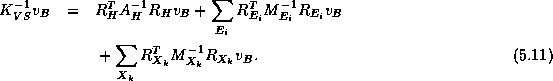
Smith
[191] proved that the condition number
of

is bounded independent of
and
, provided
there is sufficient overlap of
with
.
Next:
Further Remarks
Up:
Domain Decomposition Methods
Previous:
Overlapping Subdomain Methods
Jack Dongarra
Mon Nov 20 08:52:54 EST 1995
Further Remarks
Next:
Multiplicative Schwarz Methods
Up:
Domain Decomposition Methods
Previous:
Non-overlapping Subdomain Methods
Jack Dongarra
Mon Nov 20 08:52:54 EST 1995
Multiplicative Schwarz Methods
Next:
Inexact Solves
Up:
Further Remarks
Previous:
Further Remarks
As mentioned before,
the Additive Schwarz preconditioner can be
viewed as an overlapping block Jacobi preconditioner.
Analogously, one can define a multiplicative Schwarz
preconditioner which corresponds to a symmetric block Gauss-Seidel
version. That is, the solves on each subdomain are performed
sequentially, using the most current iterates as boundary conditions
from neighboring subdomains. Even without conjugate gradient
acceleration, the multiplicative
method can take many fewer iterations than the additive version.
However, the multiplicative version is not as parallelizable,
although the degree of parallelism can be increased
by trading off the convergence rate through
multi-coloring the subdomains.
The theory can be found in Bramble, et al.
[37].
Jack Dongarra
Mon Nov 20 08:52:54 EST 1995
Inexact Solves
Next:
Nonsymmetric Problems
Up:
Further Remarks
Previous:
Multiplicative Schwarz Methods
The exact solves involving  and
and  in
in
 can be replaced by inexact solves
 and
and  ,
which can be standard elliptic preconditioners themselves
(e.g. multigrid, ILU, SSOR, etc.).
,
which can be standard elliptic preconditioners themselves
(e.g. multigrid, ILU, SSOR, etc.).
For the Schwarz methods, the modification is straightforward
and the Inexact Solve Additive Schwarz Preconditioner
is simply:
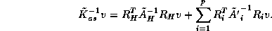
The Schur Complement methods require more changes to accommodate
inexact solves.
By replacing

by

in
the definitions of
and

, we can easily obtain
inexact preconditioners

and

for
.
The main difficulty is, however, that the evaluation of the product
requires exact subdomain solves in
.
One way to get around this
is to use an inner iteration using

as a preconditioner for

in order to compute the action
of
.
An alternative is to perform the iteration on the larger system
(
) and construct a preconditioner from the
factorization in (
) by replacing the terms

by

respectively,
where

can be either
or
.
Care must be taken to scale

and
so that they are as close to
and
as possible respectively -
it is not sufficient that the condition number of

and

be close to unity, because
the scaling of the coupling matrix

may be wrong.
Jack Dongarra
Mon Nov 20 08:52:54 EST 1995
Nonsymmetric Problems
Next:
Choice of Coarse
Up:
Further Remarks
Previous:
Inexact Solves
The preconditioners given above extend naturally to nonsymmetric
's (e.g., convection-diffusion problems), at least when the
nonsymmetric part is not too large. The nice theoretical convergence
rates can be retained provided that the coarse grid size  is chosen
small enough (depending on the size of the nonsymmetric part of
)
(see Cai and Widlund
[43]).
Practical implementations (especially for parallelism) of nonsymmetric
domain decomposition methods are discussed
in
[138]
[137].
is chosen
small enough (depending on the size of the nonsymmetric part of
)
(see Cai and Widlund
[43]).
Practical implementations (especially for parallelism) of nonsymmetric
domain decomposition methods are discussed
in
[138]
[137].
Jack Dongarra
Mon Nov 20 08:52:54 EST 1995
Choice of Coarse Grid Size <IMG ALIGN=BOTTOM SRC="http://www.netlib.org/utk/papers/templates/_22900_tex2html_wrap8189.gif">
Next:
Multigrid Methods
Up:
Further Remarks
Previous:
Nonsymmetric Problems
Given  , it has been observed empirically (see Gropp and
Keyes
[111]) that there often exists an optimal value of
which minimizes the total computational time for solving the problem.
A small
provides a better, but more expensive, coarse grid
approximation, and requires solving more, but smaller, subdomain
solves. A large
has the opposite effect. For model problems, the
optimal
can be determined for both sequential and parallel
implementations (see Chan and Shao
[53]). In
practice, it may pay to determine a near optimal value of
empirically if the preconditioner is to be re-used many times.
However, there
may also be geometric constraints on the range of values that
can
take.
, it has been observed empirically (see Gropp and
Keyes
[111]) that there often exists an optimal value of
which minimizes the total computational time for solving the problem.
A small
provides a better, but more expensive, coarse grid
approximation, and requires solving more, but smaller, subdomain
solves. A large
has the opposite effect. For model problems, the
optimal
can be determined for both sequential and parallel
implementations (see Chan and Shao
[53]). In
practice, it may pay to determine a near optimal value of
empirically if the preconditioner is to be re-used many times.
However, there
may also be geometric constraints on the range of values that
can
take.
Jack Dongarra
Mon Nov 20 08:52:54 EST 1995
Multigrid Methods
Next:
Row Projection Methods
Up:
Remaining topics
Previous:
Choice of Coarse
Multigrid method: Solution method for linear systems
based on restricting and extrapolating solutions between a series
of nested grids.
Simple iterative methods (such as the Jacobi
method) tend to damp out high frequency components of the error
fastest (see §
). This has led people to
develop methods based on the following heuristic:
- Perform some steps of a basic method in order to smooth
out the error.
- Restrict the current state of the problem to a
subset of the grid points, the so-called ``coarse grid'', and solve the
resulting projected problem.
- Interpolate the coarse grid solution back to the
original grid, and perform a number of steps of the basic method
again.
Steps 1 and 3 are called ``pre-smoothing'' and ``post-smoothing''
respectively; by applying this method recursively to step 2 it becomes
a true ``multigrid'' method. Usually the generation of subsequently
coarser grids is halted at a point where the number of variables
becomes small enough that direct solution of the linear system is feasible.
The method outlined above is said to be a ``V-cycle'' method, since it
descends through a sequence of subsequently coarser grids, and then
ascends this sequence in reverse order. A ``W-cycle'' method results
from visiting the coarse grid twice, with possibly some
smoothing steps in between.
An analysis of multigrid methods is relatively straightforward in the
case of simple differential operators such as the Poisson operator on
tensor product grids. In that case, each next coarse grid is taken to
have the double grid spacing of the previous grid. In two dimensions,
a coarse grid will have one quarter of the number of points of the
corresponding fine grid. Since the coarse grid is again a tensor
product grid, a Fourier analysis (see for instance
Briggs
[42]) can be used. For the more general case
of self-adjoint elliptic operators on arbitrary domains a more
sophisticated analysis is
needed (see Hackbusch
[117],
McCormick
[148]). Many
multigrid methods can be shown to have an (almost) optimal number of
operations, that is, the work involved is proportional to the number
of variables.
From the above description it is clear that iterative methods play a
role in multigrid theory as smoothers (see
Kettler
[133]). Conversely, multigrid-like
methods can be used as preconditioners in iterative methods. The basic
idea here is to partition the matrix on a given grid to a  structure
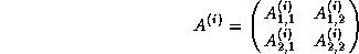
with the variables in the second block row corresponding to the coarse
grid nodes. The matrix on the next grid is then an incomplete
version of the Schur complement

The coarse grid is typically formed based on a red-black or
cyclic reduction ordering; see for
instance Rodrigue and Wolitzer
[180], and
Elman
[93].
Some multigrid preconditioners try to obtain optimality results
similar to those for the full multigrid method. Here we will merely
supply some pointers to the literature:
Axelsson and Eijkhout
[16], Axelsson and
Vassilevski
[22]
[23],
Braess
[35], Maitre and Musy
[145],
McCormick and Thomas
[149], Yserentant
[218]
and Wesseling
[215].
Next:
Row Projection Methods
Up:
Remaining topics
Previous:
Choice of Coarse
Jack Dongarra
Mon Nov 20 08:52:54 EST 1995
Convergence of the Jacobi method
Next:
The Gauss-Seidel Method
Up:
The Jacobi Method
Previous:
The Jacobi Method
Iterative methods are often used for solving discretized partial
differential equations. In that context a rigorous analysis of the
convergence of simple methods such as the Jacobi method can be given.
As an example, consider the boundary value problem

discretized by

The eigenfunctions of the  and
operator are the same:
for
and
operator are the same:
for  the function
  is an
eigenfunction corresponding to
is an
eigenfunction corresponding to  . The
eigenvalues of the Jacobi iteration matrix
are then
. The
eigenvalues of the Jacobi iteration matrix
are then
 .
.
From this it is easy to see that the high frequency modes (i.e.,
eigenfunction  with
large) are damped quickly, whereas the
damping factor for modes with
small is close to
with
large) are damped quickly, whereas the
damping factor for modes with
small is close to  . The spectral
radius of the Jacobi iteration matrix is
. The spectral
radius of the Jacobi iteration matrix is
 , and it is attained for the eigenfunction
 .
.
Spectral radius: The spectral radius of a matrix
is  .
Spectrum: The set of all eigenvalues of a matrix.
.
Spectrum: The set of all eigenvalues of a matrix.
The type of analysis applied to this example can be generalized to
higher dimensions and other stationary iterative methods. For both the
Jacobi and Gauss-Seidel method
(below) the spectral radius is found to be  where
is the
discretization mesh width, i.e.,
where
is the
discretization mesh width, i.e.,  where
where  is the
number of variables and
is the number of space dimensions.
is the
number of variables and
is the number of space dimensions.
Jack Dongarra
Mon Nov 20 08:52:54 EST 1995
Row Projection Methods
Next:
Obtaining the Software
Up:
Remaining topics
Previous:
Multigrid Methods
Most iterative methods depend on spectral properties of the
coefficient matrix, for instance some require the eigenvalues to be in
the right half plane. A class of methods without this limitation is
that of row projection methods (see Björck and
Elfving
[34], and Bramley and Sameh
[38]).
They are based on a block row partitioning of the coefficient matrix

and iterative application of orthogonal projectors

These methods have good parallel properties and seem to be robust in
handling nonsymmetric and indefinite problems.
Row projection methods can be used as
preconditioners in the conjugate gradient method. In that case, there
is a theoretical connection with the conjugate gradient method on the
normal equations (see §
).
Jack Dongarra
Mon Nov 20 08:52:54 EST 1995
Obtaining the Software
Next:
Overview of the
Up:
Templates for the Solution
Previous:
Row Projection Methods
A large body of numerical software is freely available 24 hours a day
via an electronic service called Netlib. In addition to the
template material, there are dozens of other libraries, technical
reports on various parallel computers and software, test data,
facilities to automatically translate FORTRAN programs to C, bibliographies, names and addresses of scientists and
mathematicians, and so on. One can communicate with Netlib in one of
a number of ways: by email, through anonymous ftp (netlib2.cs.utk.edu)
or
(much more easily) via the World Wide Web
through some web browser like Netscape or Mosaic.
The url for the Templates work is:
http://www.netlib.org/templates/ .
The html version of this book can be found in:
http://www.netlib.org/templates/Templates.html .
To get started using netlib, one sends a message of the form send
index to netlib@ornl.gov. A description of the entire
library should be sent to you within minutes (providing all the
intervening networks as well as the netlib server are up).
FORTRAN and C versions of the templates for each method
described in this book are available from Netlib. A user sends a
request by electronic mail as follows:
mail netlib@ornl.gov
On the subject line or in the body, single or multiple requests (one per line)
may be made as follows:
             send index from templates
             send sftemplates.shar from templates
The first request results in a return e-mail message
containing the index from the library templates, along with brief
descriptions of its contents. The second request results in a return
e-mail message consisting of a shar file containing the single
precision FORTRAN routines and a README file. The
versions of the templates that are available are listed in the table
below:
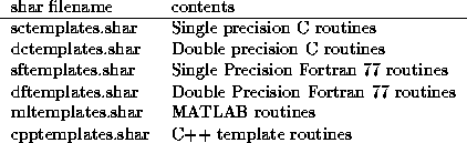
Save the mail message to a file called templates.shar. Edit the
mail header from this file and delete the lines down to and including
<< Cut Here >>. In the directory containing the shar file, type
sh templates.shar
No subdirectory will be created. The unpacked files will stay in the
current directory. Each method is written as a separate subroutine in
its own file, named after the method (e.g., CG.f, BiCGSTAB.f, GMRES.f). The argument parameters are the same
for each, with the exception of the required matrix-vector products
and preconditioner solvers (some require the transpose matrix). Also,
the amount of workspace needed varies. The details are documented in
each routine.
Note that the matrix-vector operations are accomplished using the BLAS
[144] (many manufacturers have assembly coded these
kernels for maximum performance), although a mask file is provided to
link to user defined routines.
The README file gives more details, along with instructions for
a test routine.
Next:
Overview of the
Up:
Templates for the Solution
Previous:
Row Projection Methods
Jack Dongarra
Mon Nov 20 08:52:54 EST 1995
Overview of the BLAS
Next:
Glossary
Up:
Templates for the Solution
Previous:
Obtaining the Software
The BLAS give us a standardized
set of basic codes for performing operations on vectors and matrices.
BLAS take advantage of the Fortran storage structure and the structure
of the mathematical system wherever possible. Additionally, many
computers have the BLAS library optimized to their system. Here we use
five routines:
- SCOPY: copies a vector onto another vector
- SAXPY: adds vector
(multiplied by a scalar) to vector
- SGEMV: general matrix vector product
- STRMV: matrix vector product when the matrix is triangular
- STRSV: solves
 for triangular matrix
The prefix ``S'' denotes single precision. This prefix may be
changed to ``D'', ``C'', or ``Z'', giving
the routine double, complex,
or double complex precision. (Of course, the declarations would also
have to be changed.) It is important to note that putting double precision
into single variables works, but single into double will cause errors.
If we define  a(i,j) and
= x(i), we can see what the
code is doing:
a(i,j) and
= x(i), we can see what the
code is doing:
-
ALPHA = SDOT( N, X, 1, Y, 1 ) computes the inner product of two
vectors
and
, putting the result in scalar  .
.
The corresponding Fortran segment is
ALPHA = 0.0
DO I = 1, N
  ALPHA = ALPHA  + X(I)*Y(I)
ENDDO
-
CALL SAXPY( N, ALPHA, X, 1, Y ) multiplies a
vector
of length
by the scalar  , then adds the result to
the vector
, putting the result in
.
, then adds the result to
the vector
, putting the result in
.
The corresponding Fortran segment is
DO I = 1, N
  Y(I) = ALPHA*X(I) + Y(I)
ENDDO
-
CALL SGEMV( 'N', M, N, ONE, A, LDA, X, 1, ONE, B, 1 )
computes the matrix-vector product plus vector  ,
putting the resulting vector in
,
putting the resulting vector in  .
.
The corresponding Fortran segment:
DO J = 1, N
   DO I = 1, M
      B(I) = A(I,J)*X(J) + B(I)
   ENDDO
ENDDO
This illustrates a feature of the BLAS that often requires close
attention. For example, we will use this routine to compute the residual
vector  , where
  is our current approximation to the
solution
(merely change the fourth argument to -1.0E0). Vector
will be overwritten with the residual vector; thus, if we need it later, we
will first copy it to temporary storage.
is our current approximation to the
solution
(merely change the fourth argument to -1.0E0). Vector
will be overwritten with the residual vector; thus, if we need it later, we
will first copy it to temporary storage.
-
CALL STRMV( 'U', 'N', 'N', N, A, LDA, X, 1 ) computes the
matrix-vector product  , putting the resulting vector in
,
for upper triangular matrix
.
, putting the resulting vector in
,
for upper triangular matrix
.
The corresponding Fortran segment is
DO J = 1, N
   TEMP = X(J)
   DO I = 1, J
      X(I) = X(I) + TEMP*A(I,J)
   ENDDO
ENDDO
Note that the parameters in single quotes are for descriptions
such as 'U' for `UPPER TRIANGULAR', 'N' for `No Transpose'. This
feature will be used extensively, resulting in storage savings
(among other advantages).
The variable LDA is critical for addressing the array
correctly. LDA is the leading dimension of the two-dimensional
array A,
that is, LDA is the declared (or allocated) number
of rows of the two-dimensional array
.
Next:
Glossary
Up:
Templates for the Solution
Previous:
Obtaining the Software
Jack Dongarra
Mon Nov 20 08:52:54 EST 1995
Glossary
Next:
Notation
Up:
Templates for the Solution
Previous:
Overview of the
- Adaptive methods
- Iterative methods that collect information
about the coefficient matrix during the iteration process, and use
this to speed up convergence.
- Backward error
- The size of perturbations
 of the
coefficient matrix and
of the
coefficient matrix and  of the right hand side of a linear
system
, such that the computed iterate
is the
solution of
of the right hand side of a linear
system
, such that the computed iterate
is the
solution of  .
.
- Band matrix
- A matrix
for which there are nonnegative
constants
 ,
,  such that
  if
if  or
or  . The
two constants
,
are called the left and right halfbandwidth
respectively.
. The
two constants
,
are called the left and right halfbandwidth
respectively.
- Black box
- A piece of software that can be used without
knowledge of its inner workings; the user supplies the input, and
the output is assumed to be correct.
- BLAS
- Basic Linear Algebra Subprograms; a set of commonly
occurring vector and matrix operations for dense linear algebra.
Optimized (usually assembly coded) implementations of the BLAS exist
for various computers; these will give a higher performance than
implementation in high level programming languages.
- Block factorization
- See: Block matrix operations.
- Block matrix operations
- Matrix operations expressed in terms of
submatrices.
- Breakdown
- The occurrence of a zero divisor in an iterative
method.
- Cholesky decomposition
- Expressing a symmetric matrix
as a
product of a lower triangular matrix
and its transpose
,
that is,
 .
.
- Condition number
- See: Spectral condition number.
- Convergence
- The fact whether or not, or the rate at which, an
iterative method approaches the solution of a linear system.
Convergence can be
- Linear
: some measure of the distance
to the solution decreases by a constant factor in each iteration.
- Superlinear
: the measure of the
error decreases by a growing factor.
- Smooth
: the measure of the error
decreases in all or most iterations, though not necessarily by the
same factor.
- Irregular
: the measure of the error
decreases in some iterations and increases in others. This
observation unfortunately does not imply anything about the ultimate
convergence of the method.
- Stalled
: the measure of the error
stays more or less constant during a number of iterations. As above,
this does not imply anything about the ultimate convergence of the
method.
- Dense matrix
- Matrix for which the number of zero elements is
too small to warrant specialized algorithms to exploit these zeros.
- Diagonally dominant matrix
- See: Matrix properties
- Direct method
- An algorithm that produces the solution to a
system of linear equations in a number of operations that is
determined a priori by the size of the system. In exact arithmetic,
a direct method yields the true solution to the system. See:
Iterative method.
- Distributed memory
- See: Parallel computer.
- Divergence
- An iterative method is said to diverge if it does
not converge in a reasonable number of iterations, or if some
measure of the error grows unacceptably. However, growth of the
error as such is no sign of divergence: a method with irregular
convergence behavior may ultimately converge, even though the error
grows during some iterations.
- Domain decomposition method
- Solution method for linear systems
based on a partitioning of the physical domain of the differential
equation. Domain decomposition methods typically involve (repeated)
independent system solution on the subdomains, and some way of
combining data from the subdomains on the separator part of the
domain.
- Field of values
- Given a matrix
, the field of values is the
set
 . For symmetric matrices this is the range
 .
.
- Fill
- A position that is zero in the original matrix
but not
in an exact factorization of
. In an incomplete factorization,
some fill elements are discarded.
- Forward error
- The difference between a computed iterate and the
true solution of a linear system, measured in some vector norm.
- Halfbandwidth
- See: Band matrix.
- Ill-conditioned system
- A linear system for which the
coefficient matrix has a large condition number. Since in many
applications the condition number is proportional to (some power of)
the number of unknowns, this should be understood as the constant of
proportionality being large.
- IML++
- A mathematical template library in C++
of iterative method for solving linear systems.
- Incomplete factorization
- A factorization obtained by discarding
certain elements during the factorization process (`modified' and
`relaxed' incomplete factorization compensate in some way for
discarded elements). Thus an incomplete
 factorization of a
matrix
will in general satisfy
factorization of a
matrix
will in general satisfy  ; however, one hopes
that the factorization
will be close enough to
to function
as a preconditioner in an iterative method.
; however, one hopes
that the factorization
will be close enough to
to function
as a preconditioner in an iterative method.
- Iterate
- Approximation to the solution of a linear system in any
iteration of an iterative method.
- Iterative method
- An algorithm that produces a sequence of
approximations to the solution of a linear system of equations; the
length of the sequence is not given a priori by the size of the
system. Usually, the longer one iterates, the closer one is able to
get to the true solution. See: Direct method.
- Krylov sequence
- For a given matrix
and vector
, the
sequence of vectors
 , or a finite initial part of
this sequence.
, or a finite initial part of
this sequence.
- Krylov subspace
- The subspace spanned by a Krylov sequence.
- LAPACK
- A mathematical library of linear algebra routine for
dense systems solution and eigenvalue calculations.
- Lower triangular matrix
- Matrix
for which
if
.
 factorization
- A way of writing a matrix
as a product
of a lower triangular matrix
and a unitary matrix
 , that is,
 .
.
-
factorization /
decomposition
- Expressing a matrix
as a product of a lower triangular matrix
and an upper
triangular matrix
, that is,
 .
.
-
-Matrix
- See: Matrix properties.
- Matrix norms
- See: Norms.
- Matrix properties
- We call a square matrix
- Symmetric
- if
 for all
,
.
for all
,
.
- Positive definite
- if it satisfies
 for all nonzero
vectors
.
for all nonzero
vectors
.
- Diagonally dominant
- if
 ; the
excess amount
; the
excess amount 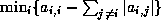 is called
the diagonal dominance of the matrix.
is called
the diagonal dominance of the matrix.
- An
-matrix
- if
 for
for  , and it is
nonsingular with
, and it is
nonsingular with  for all
,
.
for all
,
.
- Message passing
- See: Parallel computer.
- Multigrid method
- Solution method for linear systems based on
restricting and extrapolating solutions between a series of nested
grids.
- Modified incomplete factorization
- See: Incomplete
factorization.
- Mutually consistent norms
- See: Norms.
- Natural ordering
- See: Ordering of unknowns.
- Nonstationary iterative method
- Iterative method that has
iteration-dependent coefficients.
- Normal equations
- For a nonsymmetric or indefinite (but
nonsingular) system of equations
, either of the related
symmetric systems (
 ) and (
 ;
). For complex
,
is replaced with
;
). For complex
,
is replaced with  in the above
expressions.
in the above
expressions.
- Norms
- A function
 is called a vector norm
if
is called a vector norm
if
-
 for all
, and
for all
, and  only if
  .
. -
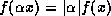 for all
  ,
.
,
.
-
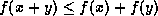 for all
,
.
for all
,
.
The same properties hold for matrix norms. A matrix norm and a
vector norm (both denoted  ) are called a mutually
consistent pair if for all matrices
and vectors
) are called a mutually
consistent pair if for all matrices
and vectors

- Ordering of unknowns
- For linear systems derived from a partial
differential equation, each unknown corresponds to a node in the
discretization mesh. Different orderings of the unknowns correspond
to permutations of the coefficient matrix. The convergence speed of
iterative methods may depend on the ordering used, and often the
parallel efficiency of a method on a parallel computer is strongly
dependent on the ordering used. Some common orderings for
rectangular domains are:
- The natural ordering; this is the consecutive numbering by
rows and columns.
- The red/black ordering; this is the numbering where all nodes
with coordinates
 for which
  is odd are numbered
before those for which
is even.
is odd are numbered
before those for which
is even.
- The ordering by diagonals; this is the ordering where nodes
are grouped in levels for which
is constant. All nodes in
one level are numbered before the nodes in the next level.
For matrices from problems on less regular domains, some common
orderings are:
- The Cuthill-McKee ordering; this starts from one point, then
numbers its neighbors, and continues numbering points that are
neighbors of already numbered points. The Reverse Cuthill-McKee
ordering then reverses the numbering; this may reduce the amount
of fill in a factorization of the matrix.
- The Minimum Degree ordering; this orders the matrix rows by
increasing numbers of nonzeros.
- Parallel computer
- Computer with multiple independent processing
units. If the processors have immediate access to the same memory,
the memory is said to be shared; if processors have private memory
that is not immediately visible to other processors, the memory is
said to be distributed. In that case, processors communicate by
message-passing.
- Pipelining
- See: Vector computer.
- Positive definite matrix
- See: Matrix properties.
- Preconditioner
- An auxiliary matrix in an iterative method that
approximates in some sense the coefficient matrix or its inverse.
The preconditioner, or preconditioning matrix, is applied in every
step of the iterative method.
- Red/black ordering
- See: Ordering of unknowns.
- Reduced system
- Linear system obtained by eliminating certain
variables from another linear system. Although the number of
variables is smaller than for the original system, the matrix of a
reduced system generally has more nonzero entries. If the original
matrix was symmetric and positive definite, then the reduced system
has a smaller condition number.
- Relaxed incomplete factorization
- See: Incomplete factorization.
- Residual
- If an iterative method is employed to solve for
in
a linear system
, then the residual corresponding to a
vector
is
 .
.
- Search direction
- Vector that is used to update an iterate.
- Shared memory
- See: Parallel computer.
- Simultaneous displacements, method of
- Jacobi method.
- Sparse matrix
- Matrix for which the number of zero elements is
large enough that algorithms avoiding operations on zero elements
pay off. Matrices derived from partial differential equations
typically have a number of nonzero elements that is proportional to
the matrix size, while the total number of matrix elements is the
square of the matrix size.
- Spectral condition number
- The product
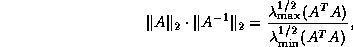
where  and
and  denote the largest and
smallest eigenvalues, respectively. For linear systems derived from
partial differential equations in 2D, the condition number is
proportional to the number of unknowns.
denote the largest and
smallest eigenvalues, respectively. For linear systems derived from
partial differential equations in 2D, the condition number is
proportional to the number of unknowns.
- Spectral radius
- The spectral radius of a matrix
is
.
- Spectrum
- The set of all eigenvalues of a matrix.
- Stationary iterative method
- Iterative method that performs in
each iteration the same operations on the current iteration vectors.
- Stopping criterion
- Since an iterative method computes
successive approximations to the solution of a linear system, a
practical test is needed to determine when to stop the iteration.
Ideally this test would measure the distance of the last iterate to
the true solution, but this is not possible. Instead, various other
metrics are used, typically involving the residual.
- Storage scheme
- The way elements of a matrix are stored in the
memory of a computer. For dense matrices, this can be the decision
to store rows or columns consecutively. For sparse matrices, common
storage schemes avoid storing zero elements; as a result they
involve indices, stored as integer data, that indicate where the
stored elements fit into the global matrix.
- Successive displacements, method of
- Gauss-Seidel method.
- Symmetric matrix
- See: Matrix properties.
- Template
- Description of an algorithm, abstracting away from
implementational details.
- Tune
- Adapt software for a specific application and computing
environment in order to obtain better performance in that case only.
itemize
- Upper triangular matrix
- Matrix
for which
if
 .
.
- Vector computer
- Computer that is able to process consecutive
identical operations (typically additions or multiplications)
several times faster than intermixed operations of different types.
Processing identical operations this way is called `pipelining' the
operations.
- Vector norms
- See: Norms.
Next:
Notation
Up:
Templates for the Solution
Previous:
Overview of the
Jack Dongarra
Mon Nov 20 08:52:54 EST 1995
Notation
Next:
References
Up:
Templates for the Solution
Previous:
Glossary
In this section, we present some of the notation we use
throughout the book.
We have tried to use standard notation that would be found
in any current publication on the subjects covered.
Throughout, we follow several conventions:
- Matrices are denoted by capital letters.
- Vectors are denoted by lowercase letters.
- Lowercase Greek letters usually denote scalars, for instance
- Matrix elements are denoted by doubly indexed lowercase letter,
however
- Matrix subblocks are denoted by doubly indexed uppercase letters.
We define matrix
of dimension  and block dimension
 as follows:
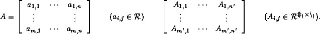
We define vector
of dimension
as follows:
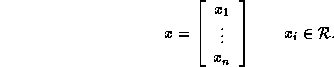
Other notation is as follows:
-
 (or simply
if the size is clear from the
context) denotes the identity matrix.
(or simply
if the size is clear from the
context) denotes the identity matrix.
-
= diag
 denotes that matrix
has elements
denotes that matrix
has elements
 on its diagonal, and zeros everywhere else.
-
 denotes the
th element of vector
during
the
th iteration
denotes the
th element of vector
during
the
th iteration
Jack Dongarra
Mon Nov 20 08:52:54 EST 1995
References
Next:
Index
Up:
Templates for the Solution
Previous:
Notation
References
-
1
-
J. AARDEN AND K.-E. KARLSSON, Preconditioned CG-type methods for
solving the coupled systems of fundamental semiconductor equations, BIT, 29
(1989), pp. 916-937.
-
2
-
L. ADAMS AND H. JORDAN, Is SOR color-blind?, SIAM J. Sci.
Statist. Comput., 7 (1986), pp. 490-506.
-
3
-
E. ANDERSON, ET. AL., LAPACK Users Guide, SIAM, Philadelphia,
1992.
-
4
-
J. APPLEYARD AND I. CHESHIRE, Nested factorization, in Reservoir
Simulation Symposium of the SPE, 1983.
Paper 12264.
-
5
-
M. ARIOLI, J. DEMMEL, AND I. DUFF, Solving sparse linear systems
with sparse backward error, SIAM J. Matrix Anal. Appl., 10 (1989),
pp. 165-190.
-
6
-
W. ARNOLDI, The principle of minimized iterations in the solution of
the matrix eigenvalue problem, Quart. Appl. Math., 9 (1951), pp. 17-29.
-
7
-
S. ASHBY, CHEBYCODE: A Fortran implementation of
Manteuffel's adaptive Chebyshev algorithm, Tech. Rep. UIUCDCS-R-85-1203,
University of Illinois, 1985.
-
8
-
S. ASHBY, T. MANTEUFFEL, AND J. OTTO, A comparison of adaptive
Chebyshev and least squares polynomial preconditioning for Hermitian
positive definite linear systems, SIAM J. Sci. Statist. Comput., 13 (1992),
pp. 1-29.
-
9
-
S. ASHBY, T. MANTEUFFEL, AND P. SAYLOR, Adaptive polynomial
preconditioning for Hermitian indefinite linear systems, BIT, 29 (1989),
pp. 583-609.
-
10
-
S. F. ASHBY, T. A. MANTEUFFEL, AND P. E. SAYLOR, A taxonomy for
conjugate gradient methods, SIAM J. Numer. Anal., 27 (1990), pp. 1542-1568.
-
11
-
C. ASHCRAFT AND R. GRIMES, On vectorizing incomplete factorizations
and SSOR preconditioners, SIAM J. Sci. Statist. Comput., 9 (1988),
pp. 122-151.
-
12
-
O. AXELSSON, Incomplete block matrix factorization preconditioning
methods. The ultimate answer?, J. Comput. Appl. Math., 12& (1985),
pp. 3-18.
-
13
-
height 2pt depth -1.6pt width 23pt, A general incomplete
block-matrix factorization method, Linear Algebra Appl., 74 (1986),
pp. 179-190.
-
14
-
O. AXELSSON AND A. BARKER, Finite element solution of boundary value
problems. Theory and computation, Academic Press, Orlando, Fl., 1984.
-
15
-
O. AXELSSON AND V. EIJKHOUT, Vectorizable preconditioners for
elliptic difference equations in three space dimensions, J. Comput. Appl.
Math., 27 (1989), pp. 299-321.
-
16
-
height 2pt depth -1.6pt width 23pt, The nested recursive
two-level factorization method for nine-point difference matrices, SIAM J.
Sci. Statist. Comput., 12 (1991), pp. 1373-1400.
-
17
-
O. AXELSSON AND I. GUSTAFSSON, Iterative solution for the solution
of the Navier equations of elasticity, Comput. Methods Appl. Mech. Engrg.,
15 (1978), pp. 241-258.
-
18
-
O. AXELSSON AND G. LINDSKOG, On the eigenvalue distribution of a
class of preconditioning matrices, Numer. Math., 48 (1986), pp. 479-498.
-
19
-
height 2pt depth -1.6pt width 23pt, On the rate of
convergence of the preconditioned conjugate gradient method, Numer. Math.,
48 (1986), pp. 499-523.
-
20
-
O. AXELSSON AND N. MUNKSGAARD, Analysis of incomplete factorizations
with fixed storage allocation, in Preconditioning Methods - Theory and
Applications, D. Evans, ed., Gordon and Breach, New York, 1983, pp. 265-293.
-
21
-
O. AXELSSON AND B. POLMAN, On approximate factorization methods for
block-matrices suitable for vector and parallel processors, Linear Algebra
Appl., 77 (1986), pp. 3-26.
-
22
-
O. AXELSSON AND P. VASSILEVSKI, Algebraic multilevel preconditioning
methods, I, Numer. Math., 56 (1989), pp. 157-177.
-
23
-
height 2pt depth -1.6pt width 23pt, Algebraic multilevel
preconditioning methods, II, SIAM J. Numer. Anal., 57 (1990),
pp. 1569-1590.
-
24
-
O. AXELSSON AND P. S. VASSILEVSKI, A black box generalized conjugate
gradient solver with inner iterations and variable-step preconditioning,
SIAM J. Matrix Anal. Appl., 12 (1991), pp. 625-644.
-
25
-
R. BANK, Marching algorithms for elliptic boundary value problems;
II: The variable coefficient case, SIAM J. Numer. Anal., 14 (1977),
pp. 950-970.
-
26
-
R. BANK, T. CHAN, W. COUGHRAN JR., AND R. SMITH, The
Alternate-Block-Factorization procedure for systems of partial
differential equations, BIT, 29 (1989), pp. 938-954.
-
27
-
R. BANK AND D. ROSE, Marching algorithms for elliptic boundary value
problems. I: The constant coefficient case, SIAM J. Numer. Anal., 14
(1977), pp. 792-829.
-
28
-
R. E. BANK AND T. F. CHAN, An analysis of the composite step
Biconjugate gradient method, Numerische Mathematik, 66 (1993),
pp. 295-319.
-
29
-
R. E. BANK AND T. F. CHAN, A composite step bi-conjugate gradient
algorithm for nonsymmetric linear systems, Numer. Alg., (1994), pp. 1-16.
-
30
-
G. BAUDET, Asynchronous iterative methods for multiprocessors, J.
Assoc. Comput. Mach., 25 (1978), pp. 226-244.
-
31
-
R. BEAUWENS, On Axelsson's perturbations, Linear Algebra Appl.,
68 (1985), pp. 221-242.
-
32
-
height 2pt depth -1.6pt width 23pt, Approximate
factorizations with S/P consistently ordered
-factors, BIT, 29
(1989), pp. 658-681.
-
33
-
R. BEAUWENS AND L. QUENON, Existence criteria for partial matrix
factorizations in iterative methods, SIAM J. Numer. Anal., 13 (1976),
pp. 615-643.
-
34
-
A. BJÖRCK AND T. ELFVING, Accelerated projection methods for
computing pseudo-inverse solutions of systems of linear equations, BIT, 19
(1979), pp. 145-163.
-
35
-
D. BRAESS, The contraction number of a multigrid method for solving
the Poisson equation, Numer. Math., 37 (1981), pp. 387-404.
-
36
-
J. H. BRAMBLE, J. E. PASCIAK, AND A. H. SCHATZ, The construction of
preconditioners for elliptic problems by substructuring, I, Mathematics of
Computation, 47 (1986), pp. 103- 134.
-
37
-
J. H. BRAMBLE, J. E. PASCIAK, J. WANG, AND J. XU, Convergence
estimates for product iterative methods with applications to domain
decompositions and multigrid, Math. Comp., 57(195) (1991), pp. 1-21.
-
38
-
R. BRAMLEY AND A. SAMEH, Row projection methods for large
nonsymmetric linear systems, SIAM J. Sci. Statist. Comput., 13 (1992),
pp. 168-193.
-
39
-
C. BREZINSKI AND H. SADOK, Avoiding breakdown in the CGS
algorithm, Numer. Alg., 1 (1991), pp. 199-206.
-
40
-
C. BREZINSKI, M. ZAGLIA, AND H. SADOK, Avoiding breakdown and near
breakdown in Lanczos type algorithms, Numer. Alg., 1 (1991), pp. 261-284.
-
41
-
height 2pt depth -1.6pt width 23pt, A breakdown free
Lanczos type algorithm for solving linear systems, Numer. Math., 63
(1992), pp. 29-38.
-
42
-
W. BRIGGS, A Multigrid Tutorial, SIAM, Philadelphia, 1977.
-
43
-
X.-C. CAI AND O. WIDLUND, Multiplicative Schwarz algorithms for
some nonsymmetric and indefinite problems, SIAM J. Numer. Anal., 30 (1993),
pp. 936-952.
-
44
-
T. CHAN, Fourier analysis of relaxed incomplete factorization
preconditioners, SIAM J. Sci. Statist. Comput., 12 (1991), pp. 668-680.
-
45
-
T. CHAN, L. DE PILLIS, AND H. VAN DER VORST, A transpose-free
squared Lanczos algorithm and application to solving nonsymmetric linear
systems, Tech. Rep. CAM 91-17, UCLA, Dept. of Math., Los Angeles, CA
90024-1555, 1991.
-
46
-
T. CHAN, E. GALLOPOULOS, V. SIMONCINI, T. SZETO, AND C. TONG, A
quasi-minimal residual variant of the Bi-CGSTAB algorithm for nonsymmetric
systems, SIAM J. Sci. Comp., 15(2) (1994), pp. 338-347.
-
47
-
T. CHAN, R. GLOWINSKI, , J. PéRIAUX, AND O. WIDLUND, eds., Domain Decomposition Methods, Philadelphia, 1989, SIAM.
Proceedings of the Second International Symposium on Domain
Decomposition Methods, Los Angeles, CA, January 14 - 16, 1988.
-
48
-
height 2pt depth -1.6pt width 23pt, eds., Domain
Decomposition Methods, Philadelphia, 1990, SIAM.
Proceedings of the Third International Symposium on Domain
Decomposition Methods, Houston, TX, 1989.
-
49
-
height 2pt depth -1.6pt width 23pt, eds., Domain
Decomposition Methods, SIAM, Philadelphia, 1991.
Proceedings of the Fourth International Symposium on Domain
Decomposition Methods, Moscow, USSR, 1990.
-
50
-
T. CHAN AND C.-C. J. KUO, Two-color Fourier analysis of iterative
algorithms for elliptic problems with red/black ordering, SIAM J. Sci.
Statist. Comput., 11 (1990), pp. 767-793.
-
51
-
T. F. CHAN AND T. MATHEW, Domain decomposition algorithms, Acta
Numerica, (1994), pp. 61-144.
-
52
-
T. F. CHAN, T. P. MATHEW, AND J. P. SHAO, Efficient variants of the
vertex space domain decomposition algorithm, SIAM J. Sci. Comput., 15(6)
(1994), pp. 1349-1374.
-
53
-
T. F. CHAN AND J. SHAO, Optimal coarse grid size in domain
decomposition, J. Comput. Math., 12(4) (1994), pp. 291-297.
-
54
-
D. CHAZAN AND W. MIRANKER, Chaotic relaxation, Linear Algebra
Appl., 2 (1969), pp. 199-222.
-
55
-
A. CHRONOPOULOS AND C. GEAR,
-step iterative methods for
symmetric linear systems, J. Comput. Appl. Math., 25 (1989), pp. 153-168.
-
56
-
P. CONCUS AND G. GOLUB, A generalized conjugate gradient method for
nonsymmetric systems of linear equations, in Computer methods in Applied
Sciences and Engineering, Second International Symposium, Dec 15-19, 1975;
Lecture Notes in Economics and Mathematical Systems, Vol. 134, Berlin, New
York, 1976, Springer-Verlag.
-
57
-
P. CONCUS, G. GOLUB, AND G. MEURANT, Block preconditioning for the
conjugate gradient method, SIAM J. Sci. Statist. Comput., 6 (1985),
pp. 220-252.
-
58
-
P. CONCUS, G. GOLUB, AND D. O'LEARY, A generalized conjugate
gradient method for the numerical solution of elliptic partial differential
equations, in Sparse Matrix Computations, J. Bunch and D. Rose, eds.,
Academic Press, New York, 1976, pp. 309-332.
-
59
-
P. CONCUS AND G. H. GOLUB, Use of fast direct methods for the
efficient numerical solution of nonseparable elliptic equations, SIAM J.
Numer. Anal., 10 (1973), pp. 1103-1120.
-
60
-
E. CUTHILL AND J. MCKEE, Reducing the bandwidth of sparse symmetric
matrices, in ACM Proceedings of the 24th National Conference, 1969.
-
61
-
E. D'AZEVEDO, V. EIJKHOUT, AND C. ROMINE, LAPACK working note 56:
Reducing communication costs in the conjugate gradient algorithm on
distributed memory multiprocessor, tech. report, Computer Science
Department, University of Tennessee, Knoxville, TN, 1993.
-
62
-
E. D'AZEVEDO AND C. ROMINE, Reducing communication costs in the
conjugate gradient algorithm on distributed memory multiprocessors, Tech.
Rep. ORNL/TM-12192, Oak Ridge National Lab, Oak Ridge, TN, 1992.
-
63
-
E. DE STURLER, A parallel restructured version of GMRES(m),
Tech. Rep. 91-85, Delft University of Technology, Delft, The Netherlands,
1991.
-
64
-
E. DE STURLER AND D. R. FOKKEMA, Nested Krylov methods and
preserving the orthogonality, Tech. Rep. Preprint 796, Utrecht University,
Utrecht, The Netherlands, 1993.
-
65
-
S. DEMKO, W. MOSS, AND P. SMITH, Decay rates for inverses of band
matrices, Mathematics of Computation, 43 (1984), pp. 491-499.
-
66
-
J. DEMMEL, The condition number of equivalence transformations that
block diagonalize matrix pencils, SIAM J. Numer. Anal., 20 (1983),
pp. 599-610.
-
67
-
J. DEMMEL, M. HEATH, AND H. VAN DER VORST, Parallel numerical linear
algebra, in Acta Numerica, Vol. 2, Cambridge Press, New York, 1993.
-
68
-
S. DOI, On parallelism and convergence of incomplete LU
factorizations, Appl. Numer. Math., 7 (1991), pp. 417-436.
-
69
-
J. DONGARRA, J. DUCROZ, I. DUFF, AND S. HAMMARLING, A set of level
3 Basic Linear Algebra Subprograms, ACM Trans. Math. Soft., 16
(1990), pp. 1-17.
-
70
-
J. DONGARRA, J. DUCROZ, S. HAMMARLING, AND R. HANSON, An extended
set of FORTRAN Basic Linear Algebra Subprograms, ACM Trans. Math.
Soft., 14 (1988), pp. 1-32.
-
71
-
J. DONGARRA, I. DUFF, D. SORENSEN, AND H. VAN DER VORST, Solving
Linear Systems on Vector and Shared Memory Computers, SIAM, Philadelphia,
PA, 1991.
-
72
-
J. DONGARRA AND E. GROSSE, Distribution of mathematical software via
electronic mail, Comm. ACM, 30 (1987), pp. 403-407.
-
73
-
J. DONGARRA, C. MOLER, J. BUNCH, AND G. STEWART, LINPACK Users'
Guide, SIAM, Philadelphia, 1979.
-
74
-
J. DONGARRA AND H. VAN DER VORST, Performance of various computers
using standard sparse linear equations solving techniques, in Computer
Benchmarks, J. Dongarra and W. Gentzsch, eds., Elsevier Science Publishers
B.V., New York, 1993, pp. 177-188.
-
75
-
F. DORR, The direct solution of the discrete Poisson equation on a
rectangle, SIAM Rev., 12 (1970), pp. 248-263.
-
76
-
M. DRYJA AND O. B. WIDLUND, Towards a unified theory of domain
decomposition algorithms for elliptic problems, Tech. Rep. 486, also
Ultracomputer Note 167, Department of Computer Science, Courant Institute,
1989.
-
77
-
D. DUBOIS, A. GREENBAUM, AND G. RODRIGUE, Approximating the inverse
of a matrix for use in iterative algorithms on vector processors, Computing,
22 (1979), pp. 257-268.
-
78
-
I. DUFF, R. GRIMES, AND J. LEWIS, Sparse matrix test problems, ACM
Trans. Math. Soft., 15 (1989), pp. 1-14.
-
79
-
I. DUFF AND G. MEURANT, The effect of ordering on preconditioned
conjugate gradients, BIT, 29 (1989), pp. 635-657.
-
80
-
I. S. DUFF, A. M. ERISMAN, AND J.K.REID, Direct methods for sparse
matrices, Oxford University Press, London, 1986.
-
81
-
T. DUPONT, R. KENDALL, AND H. RACHFORD, An approximate factorization
procedure for solving self-adjoint elliptic difference equations, SIAM J.
Numer. Anal., 5 (1968), pp. 559-573.
-
82
-
E. D'YAKONOV, The method of variable directions in solving systems
of finite difference equations, Soviet Math. Dokl., 2 (1961), pp. 577-580.
TOM 138, 271-274.
-
83
-
L. EHRLICH, An Ad-Hoc SOR method, J. Comput. Phys., 43 (1981),
pp. 31-45.
-
84
-
M. EIERMANN AND R. VARGA, Is the optimal
best for the SOR
iteration method?, Linear Algebra Appl., 182 (1993), pp. 257-277.
-
85
-
V. EIJKHOUT, Analysis of parallel incomplete point factorizations,
Linear Algebra Appl., 154-156 (1991), pp. 723-740.
-
86
-
height 2pt depth -1.6pt width 23pt, Beware of
unperturbed modified incomplete point factorizations, in Proceedings of the
IMACS International Symposium on Iterative Methods in Linear Algebra,
Brussels, Belgium, R. Beauwens and P. de Groen, eds., 1992.
-
87
-
height 2pt depth -1.6pt width 23pt, LAPACK working
note 50: Distributed sparse data structures for linear algebra operations,
Tech. Rep. CS 92-169, Computer Science Department, University of Tennessee,
Knoxville, TN, 1992.
-
88
-
height 2pt depth -1.6pt width 23pt, LAPACK working
note 51: Qualitative properties of the conjugate gradient and Lanczos
methods in a matrix framework, Tech. Rep. CS 92-170, Computer Science
Department, University of Tennessee, Knoxville, TN, 1992.
-
89
-
V. EIJKHOUT AND B. POLMAN, Decay rates of inverses of banded
-matrices that are near to Toeplitz matrices, Linear Algebra Appl.,
109 (1988), pp. 247-277.
-
90
-
V. EIJKHOUT AND P. VASSILEVSKI, Positive definiteness aspects of
vectorizable preconditioners, Parallel Computing, 10 (1989), pp. 93-100.
-
91
-
S. EISENSTAT, Efficient implementation of a class of preconditioned
conjugate gradient methods, SIAM J. Sci. Statist. Comput., 2 (1981),
pp. 1-4.
-
92
-
R. ELKIN, Convergence theorems for Gauss-Seidel and other
minimization algorithms, Tech. Rep. 68-59, Computer Science Center,
University of Maryland, College Park, MD, Jan. 1968.
-
93
-
H. ELMAN, Approximate Schur complement preconditioners on serial
and parallel computers, SIAM J. Sci. Statist. Comput., 10 (1989),
pp. 581-605.
-
94
-
H. ELMAN AND M. SCHULTZ, Preconditioning by fast direct methods for
non self-adjoint nonseparable elliptic equations, SIAM J. Numer. Anal., 23
(1986), pp. 44-57.
-
95
-
L. ELSNER, A note on optimal block-scaling of matrices, Numer.
Math., 44 (1984), pp. 127-128.
-
96
-
V. FABER AND T. MANTEUFFEL, Necessary and sufficient conditions for
the existence of a conjugate gradient method, SIAM J. Numer. Anal., 21
(1984), pp. 315-339.
-
97
-
G. FAIRWEATHER, A. GOURLAY, AND A. MITCHELL, Some high accuracy
difference schemes with a splitting operator for equations of parabolic and
elliptic type, Numer. Math., 10 (1967), pp. 56-66.
-
98
-
R. FLETCHER, Conjugate gradient methods for indefinite systems, in
Numerical Analysis Dundee 1975, G. Watson, ed., Berlin, New York, 1976,
Springer Verlag, pp. 73-89.
-
99
-
G. FORSYTHE AND E. STRAUSS, On best conditioned matrices, Proc.
Amer. Math. Soc., 6 (1955), pp. 340-345.
-
100
-
R. FREUND, Conjugate gradient-type methods for linear systems with
complex symmetric coefficient matrices, SIAM J. Sci. Statist. Comput., 13
(1992), pp. 425-448.
-
101
-
R. FREUND, M. GUTKNECHT, AND N. NACHTIGAL, An implementation of the
look-ahead Lanczos algorithm for non-Hermitian matrices, SIAM J. Sci.
Comput., 14 (1993), pp. 137-158.
-
102
-
R. FREUND AND N. NACHTIGAL, QMR: A quasi-minimal residual method
for non-Hermitian linear systems, Numer. Math., 60 (1991), pp. 315-339.
-
103
-
height 2pt depth -1.6pt width 23pt, An implementation of
the QMR method based on coupled two-term recurrences, SIAM J. Sci.
Statist. Comput., 15 (1994), pp. 313-337.
-
104
-
R. FREUND AND T. SZETO, A quasi-minimal residual squared algorithm
for non-Hermitian linear systems, Tech. Rep. CAM Report 92-19, UCLA Dept.
of Math., 1992.
-
105
-
R. W. FREUND, A transpose-free quasi-minimum residual algorithm for
non-Hermitian linear systems, SIAM J. Sci. Comput., 14 (1993),
pp. 470-482.
-
106
-
R. W. FREUND, G. H. GOLUB, AND N. M. NACHTIGAL, Iterative solution
of linear systems, Acta Numerica, (1992), pp. 57-100.
-
107
-
R. GLOWINSKI, G. H. GOLUB, G. A. MEURANT, AND J. PéRIAUX, eds., Domain Decomposition Methods for Partial Differential Equations, SIAM,
Philadelphia, 1988.
Proceedings of the First International Symposium on Domain
Decomposition Methods for Partial Differential Equations, Paris,
France, January 1987.
-
108
-
G. GOLUB AND D. O'LEARY, Some history of the conjugate gradient and
Lanczos methods, SIAM Rev., 31 (1989), pp. 50-102.
-
109
-
G. GOLUB AND C. VAN LOAN, Matrix Computations, second
edition, The Johns Hopkins University Press, Baltimore, 1989.
-
110
-
A. GREENBAUM AND Z. STRAKOS, Predicting the behavior of finite
precision Lanczos and conjugate gradient computations, SIAM J. Mat.
Anal. Appl., 13 (1992), pp. 121-137.
-
111
-
W. D. GROPP AND D. E. KEYES, Domain decomposition with local mesh
refinement, SIAM J. Sci. Statist. Comput., 13 (1992), pp. 967-993.
-
112
-
I. GUSTAFSSON, A class of first-order factorization methods, BIT,
18 (1978), pp. 142-156.
-
113
-
M. H. GUTKNECHT, The unsymmetric Lanczos algorithms and their
relations to Páde approximation, continued fractions and the QD
algorithm, in Proceedings of the Copper Mountain Conference on Iterative
Methods, 1990.
-
114
-
height 2pt depth -1.6pt width 23pt, A completed theory
of the unsymmetric Lanczos process and related algorithms, part I, SIAM
J. Matrix Anal. Appl., 13 (1992), pp. 594-639.
-
115
-
height 2pt depth -1.6pt width 23pt, Variants of
Bi-CGSTAB for matrices with complex spectrum, SIAM J. Sci. Comp., 14
(1993), pp. 1020-1033.
-
116
-
height 2pt depth -1.6pt width 23pt, A completed theory
of the unsymmetric Lanczos process and related algorithms, part II, SIAM
J. Matrix Anal. Appl., 15 (1994), pp. 15-58.
-
117
-
W. HACKBUSCH, Multi-Grid Methods and Applications, Springer-Verlag,
Berlin, New York, 1985.
-
118
-
height 2pt depth -1.6pt width 23pt, Iterative Lösung
großer schwachbesetzter Gleichungssysteme, Teubner, Stuttgart, 1991.
-
119
-
A. HADJIDIMOS, On some high accuracy difference schemes for solving
elliptic equations, Numer. Math., 13 (1969), pp. 396-403.
-
120
-
L. HAGEMAN AND D. YOUNG, Applied Iterative Methods, Academic Press,
New York, 1981.
-
121
-
W. HAGER, Condition estimators, SIAM J. Sci. Statist. Comput., 5
(1984), pp. 311-316.
-
122
-
M. HESTENES AND E. STIEFEL, Methods of conjugate gradients for
solving linear systems, J. Res. Nat. Bur. Stand., 49 (1952), pp. 409-436.
-
123
-
M. R. HESTENES, Conjugacy and gradients, in A History of Scientific
Computing, Addison-Wesley, Reading, MA, 1990, pp. 167-179.
-
124
-
N. HIGHAM, Experience with a matrix norm estimator, SIAM J. Sci.
Statist. Comput., 11 (1990), pp. 804-809.
-
125
-
K. JEA AND D. YOUNG, Generalized conjugate-gradient acceleration of
nonsym- metrizable iterative methods, Linear Algebra Appl., 34 (1980),
pp. 159-194.
-
126
-
O. JOHNSON, C. MICCHELLI, AND G. PAUL, Polynomial preconditioning
for conjugate gradient calculation, SIAM J. Numer. Anal., 20 (1983),
pp. 362-376.
-
127
-
M. JONES AND P. PLASSMANN, Parallel solution of unstructed, sparse
systems of linear equations, in Proceedings of the Sixth SIAM conference on
Parallel Processing for Scientific Computing, R. Sincovec, D. Keyes,
M. Leuze, L. Petzold, and D. Reed, eds., SIAM, Philadelphia, pp. 471-475.
-
128
-
height 2pt depth -1.6pt width 23pt, A parallel graph
coloring heuristic, SIAM J. Sci. Statist. Comput., 14 (1993), pp. 654-669.
-
129
-
W. JOUBERT, Lanczos methods for the solution of nonsymmetric systems
of linear equations, SIAM J. Matrix Anal. Appl., 13 (1992), pp. 926-943.
-
130
-
W. KAHAN, Gauss-Seidel methods of solving large systems of linear
equations, PhD thesis, University of Toronto, 1958.
-
131
-
S. KANIEL, Estimates for some computational techniques in linear
algebra, Mathematics of Computation, 20 (1966), pp. 369-378.
-
132
-
D. KERSHAW, The incomplete Cholesky-conjugate gradient method for
the iterative solution of systems of linear equations, J. Comput. Phys., 26
(1978), pp. 43-65.
-
133
-
R. KETTLER, Analysis and comparison of relaxation schemes in robust
multigrid and preconditioned conjugate gradient methods, in Multigrid
Methods, Lecture Notes in Mathematics 960, W. Hackbusch and U. Trottenberg,
eds., Springer-Verlag, Berlin, New York, 1982, pp. 502-534.
-
134
-
height 2pt depth -1.6pt width 23pt, Linear multigrid
methods in numerical reservoir simulation, PhD thesis, Delft University of
Technology, Delft, The Netherlands, 1987.
-
135
-
D. E. KEYES, T. F. CHAN, G. MEURANT, J. S. SCROGGS, AND R. G. VOIGT,
eds., Domain Decomposition Methods For Partial Differential Equations,
SIAM, Philadelphia, 1992.
Proceedings of the Fifth International Symposium on Domain
Decomposition Methods, Norfolk, VA, 1991.
-
136
-
D. E. KEYES AND W. D. GROPP, A comparison of domain decomposition
techniques for elliptic partial differential equations and their parallel
implementation, SIAM J. Sci. Statist. Comput., 8 (1987), pp. s166 - s202.
-
137
-
height 2pt depth -1.6pt width 23pt, Domain decomposition
for nonsymmetric systems of equations: Examples from computational fluid
dynamics, in Domain Decomposition Methods, proceedings of the Second
Internation Symposium, Los Angeles, California, January 14-16, 1988, T. F.
Chan, R. Glowinski, J. Periaux, and O. B. Widlund, eds., Philadelphia, 1989,
SIAM, pp. 373-384.
-
138
-
height 2pt depth -1.6pt width 23pt, Domain decomposition
techniques for the parallel solution of nonsymmetric systems of elliptic
boundary value problems, Applied Num. Math., 6 (1989/1990), pp. 281-301.
-
139
-
S. K. KIM AND A. T. CHRONOPOULOS, A class of Lanczos-like
algorithms implemented on parallel computers, Parallel Comput., 17 (1991),
pp. 763-778.
-
140
-
D. R. KINCAID, J. R. RESPESS, D. M. YOUNG, AND R. G. GRIMES, ITPACK 2C: A Fortran package for solving large sparse linear systems
by adaptive accelerated iterative methods, ACM Trans. Math. Soft., 8 (1982),
pp. 302-322.
Algorithm 586.
-
141
-
L. Y. KOLOTILINA AND A. Y. YEREMIN, On a family of two-level
preconditionings of the incomlete block factorization type, Sov. J. Numer.
Anal. Math. Modelling, (1986), pp. 293-320.
-
142
-
C. LANCZOS, An iteration method for the solution of the eigenvalue
problem of linear differential and integral operators, J. Res. Nat. Bur.
Stand., 45 (1950), pp. 255-282.
-
143
-
height 2pt depth -1.6pt width 23pt, Solution of systems
of linear equations by minimized iterations, J. Res. Nat. Bur. Stand., 49
(1952), pp. 33-53.
-
144
-
C. LAWSON, R. HANSON, D. KINCAID, AND F. KROGH, Basic Linear
Algebra Subprograms for FORTRAN usage, ACM Trans. Math. Soft., 5
(1979), pp. 308-325.
-
145
-
J. MAITRE AND F. MUSY, The contraction number of a class of
two-level methods; an exact evaluation for some finite element subspaces and
model problems, in Multigrid methods, Proceedings, Köln-Porz, 1981,
W. Hackbusch and U. Trottenberg, eds., vol. 960 of Lecture Notes in
Mathematics, 1982, pp. 535-544.
-
146
-
T. MANTEUFFEL, The Tchebychev iteration for nonsymmetric linear
systems, Numer. Math., 28 (1977), pp. 307-327.
-
147
-
height 2pt depth -1.6pt width 23pt, An incomplete
factorization technique for positive definite linear systems, Mathematics of
Computation, 34 (1980), pp. 473-497.
-
148
-
S. MCCORMICK, Multilevel Adaptive Methods for Partial Differential
Equations, SIAM, Philadelphia, 1989.
-
149
-
S. MCCORMICK AND J. THOMAS, The Fast Adaptive Composite grid
(FAC) method for elliptic equations, Mathematics of Computation, 46
(1986), pp. 439-456.
-
150
-
U. MEIER AND A. SAMEH, The behavior of conjugate gradient algorithms
on a multivector processor with a hierarchical memory, J. Comput. Appl.
Math., 24 (1988), pp. 13-32.
-
151
-
U. MEIER-YANG, Preconditioned conjugate gradient-like methods for
nonsymmetric linear systems, tech. rep., CSRD, University of Illinois,
Urbana, IL, April 1992.
-
152
-
J. MEIJERINK AND H. VAN DER VORST, An iterative solution method for
linear systems of which the coefficient matrix is a symmetric
-matrix,
Mathematics of Computation, 31 (1977), pp. 148-162.
-
153
-
height 2pt depth -1.6pt width 23pt, Guidelines for the
usage of incomplete decompositions in solving sets of linear equations as
they occur in practical problems, J. Comput. Phys., 44 (1981), pp. 134-155.
-
154
-
R. MELHEM, Toward efficient implementation of preconditioned
conjugate gradient methods on vector supercomputers, Internat. J.
Supercomput. Appls., 1 (1987), pp. 77-98.
-
155
-
G. MEURANT, The block preconditioned conjugate gradient method on
vector computers, BIT, 24 (1984), pp. 623-633.
-
156
-
height 2pt depth -1.6pt width 23pt, Multitasking the
conjugate gradient method on the CRAY X-MP/48, Parallel Comput., 5
(1987), pp. 267-280.
-
157
-
N. MUNKSGAARD, Solving sparse symmetric sets of linear equations by
preconditioned conjugate gradients, ACM Trans. Math. Software, 6 (1980),
pp. 206-219.
-
158
-
N. NACHTIGAL, S. REDDY, AND L. TREFETHEN, How fast are nonsymmetric
matrix iterations?, SIAM J. Matrix Anal. Appl., 13 (1992), pp. 778-795.
-
159
-
N. NACHTIGAL, L. REICHEL, AND L. TREFETHEN, A hybrid GMRES
algorithm for nonsymmetric matrix iterations, SIAM J. Sci. Statist. Comput.,
13 (1992), pp. 796-825.
-
160
-
N. M. NACHTIGAL, A Look-Ahead Variant of the Lanczos Algorithm and
its Application to the Quasi-Minimal Residual Methods for Non-Hermitian
Linear Systems, PhD thesis, MIT, Cambridge, MA, 1991.
-
161
-
Y. NOTAY, Solving positive (semi)definite linear systems by
preconditioned iterative methods, in Preconditioned Conjugate Gradient
Methods, O. Axelsson and L. Kolotilina, eds., vol. 1457 of Lecture Notes in
Mathematics, Nijmegen, 1989, pp. 105-125.
-
162
-
height 2pt depth -1.6pt width 23pt, On the robustness of
modified incomplete factorization methods, Internat. J. Comput. Math., 40
(1992), pp. 121-141.
-
163
-
D. O'LEARY, The block conjugate gradient algorithm and related
methods, Linear Algebra Appl., 29 (1980), pp. 293-322.
-
164
-
height 2pt depth -1.6pt width 23pt, Ordering schemes for
parallel processing of certain mesh problems, SIAM J. Sci. Statist. Comput.,
5 (1984), pp. 620-632.
-
165
-
T. C. OPPE, W. D. JOUBERT, AND D. R. KINCAID, NSPCG user's guide,
version 1.0: A package for solving large sparse linear systems by various
iterative methods, Tech. Rep. CNA-216, Center for Numerical Analysis,
University of Texas at Austin, Austin, TX, April 1988.
-
166
-
J. M. ORTEGA, Introduction to Parallel and Vector Solution of Linear
Systems, Plenum Press, New York and London, 1988.
-
167
-
C. PAIGE, B. PARLETT, AND H. VAN DER VORST, Approximate solutions
and eigenvalue bounds from Krylov subspaces, Numer. Lin. Alg. Appls., 29
(1995), pp. 115-134.
-
168
-
C. PAIGE AND M. SAUNDERS, Solution of sparse indefinite systems of
linear equations, SIAM J. Numer. Anal., 12 (1975), pp. 617-629.
-
169
-
C. C. PAIGE AND M. A. SAUNDERS, LSQR: An algorithm for sparse
linear equations and sparse least squares, ACM Trans. Math. Soft., 8 (1982),
pp. 43-71.
-
170
-
G. PAOLINI AND G. RADICATI DI BROZOLO, Data structures to
vectorize CG algorithms for general sparsity patterns, BIT, 29 (1989),
pp. 703-718.
-
171
-
B. PARLETT, The symmetric eigenvalue problem, Prentice-Hall,
London, 1980.
-
172
-
B. N. PARLETT, D. R. TAYLOR, AND Z. A. LIU, A look-ahead Lanczos
algorithm for unsymmetric matrices, Mathematics of Computation, 44 (1985),
pp. 105-124.
-
173
-
D. PEACEMAN AND J. H.H. RACHFORD, The numerical solution of
parabolic and elliptic differential equations, J. Soc. Indust. Appl. Math.,
3 (1955), pp. 28-41.
-
174
-
C. POMMERELL, Solution of Large Unsymmetric Systems of Linear
Equations, vol. 17 of Series in Micro-electronics, volume 17, Hartung-Gorre
Verlag, Konstanz, 1992.
-
175
-
height 2pt depth -1.6pt width 23pt, Solution of large
unsymmetric systems of linear equations, PhD thesis, Swiss Federal Institute
of Technology, Zürich, Switzerland, 1992.
-
176
-
E. POOLE AND J. ORTEGA, Multicolor ICCG methods for vector
computers, Tech. Rep. RM 86-06, Department of Applied Mathematics,
University of Virginia, Charlottesville, VA, 1986.
-
177
-
A. QUARTERONI, J. PERIAUX, Y. KUZNETSOV, AND O. WIDLUND, eds., Domain Decomposition Methods in Science and Engineering,, vol. Contemporary
Mathematics 157, Providence, RI, 1994, AMS.
Proceedings of the Sixth International Symposium on Domain
Decomposition Methods, June 15-19, 1992, Como, Italy,.
-
178
-
G. RADICATI DI BROZOLO AND Y. ROBERT, Vector and parallel
CG-like algorithms for sparse non-symmetric systems, Tech. Rep. 681-M,
IMAG/TIM3, Grenoble, France, 1987.
-
179
-
J. REID, On the method of conjugate gradients for the solution of
large sparse systems of linear equations, in Large Sparse Sets of Linear
Equations, J. Reid, ed., Academic Press, London, 1971, pp. 231-254.
-
180
-
G. RODRIGUE AND D. WOLITZER, Preconditioning by incomplete block
cyclic reduction, Mathematics of Computation, 42 (1984), pp. 549-565.
-
181
-
Y. SAAD, The Lanczos biorthogonalization algorithm and other
oblique projection methods for solving large unsymmetric systems, SIAM J.
Numer. Anal., 19 (1982), pp. 485-506.
-
182
-
height 2pt depth -1.6pt width 23pt, Practical use of
some Krylov subspace methods for solving indefinite and nonsymmetric linear
systems, SIAM J. Sci. Statist. Comput., 5 (1984), pp. 203-228.
-
183
-
height 2pt depth -1.6pt width 23pt, Practical use of
polynomial preconditionings for the conjugate gradient method, SIAM J. Sci.
Statist. Comput., 6 (1985), pp. 865-881.
-
184
-
height 2pt depth -1.6pt width 23pt, Preconditioning
techniques for indefinite and nonsymmetric linear systems, J. Comput. Appl.
Math., 24 (1988), pp. 89-105.
-
185
-
height 2pt depth -1.6pt width 23pt, Krylov subspace
methods on supercomputers, SIAM J. Sci. Statist. Comput., 10 (1989),
pp. 1200-1232.
-
186
-
height 2pt depth -1.6pt width 23pt, SPARSKIT: A basic
tool kit for sparse matrix computation, Tech. Rep. CSRD TR 1029, CSRD,
University of Illinois, Urbana, IL, 1990.
-
187
-
height 2pt depth -1.6pt width 23pt, A flexible
inner-outer preconditioned GMRES algorithm, SIAM J. Sci. Comput., 14
(1993), pp. 461-469.
-
188
-
Y. SAAD AND M. SCHULTZ, Conjugate gradient-like algorithms for
solving nonsymmetric linear systems, Mathematics of Computation, 44 (1985),
pp. 417-424.
-
189
-
height 2pt depth -1.6pt width 23pt, GMRES: A
generalized minimal residual algorithm for solving nonsymmetric linear
systems, SIAM J. Sci. Statist. Comput., 7 (1986), pp. 856-869.
-
190
-
G. L. G. SLEIJPEN AND D. R. FOKKEMA, Bi-CGSTAB(
 ) for linear
equations involving unsymmetric matrices with complex spectrum, Elec. Trans.
Numer. Anal., 1 (1993), pp. 11-32.
) for linear
equations involving unsymmetric matrices with complex spectrum, Elec. Trans.
Numer. Anal., 1 (1993), pp. 11-32.
-
191
-
B. F. SMITH, Domain decomposition algorithms for partial
differential equations of linear elasticity, Tech. Rep. 517, Department of
Computer Science, Courant Institute, 1990.
-
192
-
P. SONNEVELD, CGS, a fast Lanczos-type solver for nonsymmetric
linear systems, SIAM J. Sci. Statist. Comput., 10 (1989), pp. 36-52.
-
193
-
R. SOUTHWELL, Relaxation Methods in Theoretical Physics, Clarendon
Press, Oxford, 1946.
-
194
-
H. STONE, Iterative solution of implicit approximations of
multidimensional partial differential equations, SIAM J. Numer. Anal., 5
(1968), pp. 530-558.
-
195
-
P. SWARZTRAUBER, The methods of cyclic reduction, Fourier analysis
and the FACR algorithm for the discrete solution of Poisson's equation on
a rectangle, SIAM Rev., 19 (1977), pp. 490-501.
-
196
-
P. L. TALLEC, Domain decomposition methods in computational
mechanics, Computational Mechanics Advances, 1994.
-
197
-
C. TONG, A comparative study of preconditioned Lanczos methods for
nonsymmetric linear systems, Tech. Rep. SAND91-8240, Sandia Nat. Lab.,
Livermore, CA, 1992.
-
198
-
A. VAN DER SLUIS, Condition numbers and equilibration of matrices,
Numer. Math., 14 (1969), pp. 14-23.
-
199
-
A. VAN DER SLUIS AND H. VAN DER VORST, The rate of convergence of
conjugate gradients, Numer. Math., 48 (1986), pp. 543-560.
-
200
-
H. VAN DER VORST, Iterative solution methods for certain sparse
linear systems with a non-symmetric matrix arising from PDE-problems, J.
Comput. Phys., 44 (1981), pp. 1-19.
-
201
-
height 2pt depth -1.6pt width 23pt, A vectorizable
variant of some ICCG methods, SIAM J. Sci. Statist. Comput., 3 (1982),
pp. 350-356.
-
202
-
height 2pt depth -1.6pt width 23pt, Large tridiagonal
and block tridiagonal linear systems on vector and parallel computers,
Parallel Comput., 5 (1987), pp. 45-54.
-
203
-
height 2pt depth -1.6pt width 23pt, (M)ICCG for 2D
problems on vector computers, in Supercomputing, A.Lichnewsky and C.Saguez,
eds., North-Holland, 1988.
-
204
-
height 2pt depth -1.6pt width 23pt, High performance
preconditioning, SIAM J. Sci. Statist. Comput., 10 (1989), pp. 1174-1185.
-
205
-
height 2pt depth -1.6pt width 23pt, ICCG and related
methods for 3D problems on vector computers, Computer Physics
Communications, 53 (1989), pp. 223-235.
-
206
-
height 2pt depth -1.6pt width 23pt, The convergence
behavior of preconditioned CG and CG-S in the presence of rounding
errors, in Preconditioned Conjugate Gradient Methods, O. Axelsson and L. Y.
Kolotilina, eds., vol. 1457 of Lecture Notes in Mathematics, Berlin, New
York, 1990, Springer-Verlag.
-
207
-
height 2pt depth -1.6pt width 23pt, Bi-CGSTAB: A
fast and smoothly converging variant of Bi-CG for the solution of
nonsymmetric linear systems, SIAM J. Sci. Statist. Comput., 13 (1992),
pp. 631-644.
-
208
-
H. VAN DER VORST AND J. MELISSEN, A Petrov-Galerkin type method
for solving
where
is symmetric complex, IEEE Trans.
Magnetics, 26 (1990), pp. 706-708.
-
209
-
H. VAN DER VORST AND C. VUIK, GMRESR: A family of nested GMRES
methods, Numer. Lin. Alg. Applic., 1 (1994), pp. 369-386.
-
210
-
J. VAN ROSENDALE, Minimizing inner product data dependencies in
conjugate gradient iteration, Tech. Rep. 172178, ICASE, NASA Langley
Research Center, 1983.
-
211
-
R. VARGA, Matrix Iterative Analysis, Prentice-Hall Inc., Englewood
Cliffs, NJ, 1962.
-
212
-
P. VASSILEVSKI, Preconditioning nonsymmetric and indefinite finite
element matrices, J. Numer. Alg. Appl., 1 (1992), pp. 59-76.
-
213
-
V. VOEVODIN, The problem of non-self-adjoint generalization of the
conjugate gradient method is closed, U.S.S.R. Comput. Maths. and Math.
Phys., 23 (1983), pp. 143-144.
-
214
-
H. F. WALKER, Implementation of the GMRES method using
Householder transformations, SIAM J. Sci. Statist. Comput., 9 (1988),
pp. 152-163.
-
215
-
P. WESSELING, An Introduction to Multigrid Methods, Wiley,
Chichester, 1991.
-
216
-
O. WIDLUND, A Lanczos method for a class of non-symmetric systems
of linear equations, SIAM J. Numer. Anal., 15 (1978), pp. 801-812.
-
217
-
D. YOUNG, Iterative solution of large linear systems, Academic
Press, New York, 1971.
-
218
-
H. YSERENTANT, On the multilevel splitting of finite element
spaces, Numer. Math., 49 (1986), pp. 379-412.
=0pt plus 40pt
Jack Dongarra
Mon Nov 20 08:52:54 EST 1995
Index
Next:
About this document
Up:
Templates for the Solution
Previous:
References
- ad hoc SOR method
- seemethod, ad hoc SOR
- asynchronous method
- seemethod, asynchronous
- Bi-CGSTAB method
- seemethod, Bi-CGSTAB
- Bi-Conjugate Gradient Stabilized method
- seemethod, Bi-CGSTAB
- bi-orthogonality
- in BiCG
-
BiConjugate Gradient (BiCG)
- in QMR
-
Quasi-Minimal Residual (QMR)
- BiCG method
- seemethod, BiCG
- BiConjugate Gradient method
- seemethod, BiCG
- BLAS
-
Why Use Templates?
- BLAS
-
CRS-based Factorization Solve
- block methods
- (, )
- breakdown
- avoiding by look-ahead
-
Convergence
- in Bi-CGSTAB
-
Convergence
- in BiCG
-
Convergence,
Convergence,
Convergence,
Quasi-Minimal Residual (QMR)
- in BiCG
-
Convergence,
Convergence,
Convergence,
Quasi-Minimal Residual (QMR)
- in BiCG
-
Convergence,
Convergence,
Convergence,
Quasi-Minimal Residual (QMR)
- in BiCG
-
Convergence,
Convergence,
Convergence,
Quasi-Minimal Residual (QMR)
- in CG for indefinite systems
-
MINRES and SYMMLQ
- CG method
- seemethod, CG
- CGNE method
- seemethod, CGNE
- CGNR method
- seemethod, CGNR
- CGS method
- seemethod, CGS
- chaotic method
- seemethod, asynchronous
- Chebyshev iteration
- seemethod, Chebyshev iteration
- codes
- C++
-
Why Use Templates?
- FORTRAN
-
Why Use Templates?
- MATLAB
-
Why Use Templates?
- complex systems
- (, )
- Conjugate Gradient method
- seemethod, CG
- Conjugate Gradient Squared method
- seemethod, CGS
- convergence
- irregular
-
Glossary
- irregular
-
Glossary
- irregular
-
Glossary
- irregular
-
Glossary
- irregular
-
Glossary
- irregular
-
Glossary
- linear
-
Glossary
- of Bi-CGSTAB
- (, )
- of Bi-CGSTAB
- (, )
- of BiCG
- (, )
- of BiCG
- (, )
- of CG
- (, )
- of CG
- (, )
- of CGNR and CGNE
-
Theory
- of CGS
- (, )
- of CGS
- (, )
- of Chebyshev iteration
- (, )
- of Chebyshev iteration
- (, )
- of Gauss-Seidel
-
The Gauss-Seidel Method
- of Jacobi
- (, )
- of Jacobi
- (, )
- of MINRES
-
MINRES and SYMMLQ
- of QMR
- (, )
- of QMR
- (, )
- of SSOR
-
The Symmetric Successive
- smooth
-
Glossary
- smooth
-
Glossary
- stalled
-
Glossary
- stalled
-
Glossary
- stalled
-
Glossary
- superlinear
-
Glossary
- superlinear
-
Glossary
- superlinear
-
Glossary
- superlinear
-
Glossary
- data structures
- (, )
- diffusion
- artificial
-
Modified incomplete factorizations
- domain decomposition
- multiplicative Schwarz
- (, )
- multiplicative Schwarz
- (, )
- non-overlapping subdomains
- (, )
- non-overlapping subdomains
- (, )
- overlapping subdomains
- (, )
- overlapping subdomains
- (, )
- Schur complement
-
Domain Decomposition Methods
- Schwarz
-
Domain Decomposition Methods
- fill-in strategies
- seepreconditioners, point incomplete"factorizations
- FORTRAN codes
- seecodes, FORTRAN
- Gauss-Seidel method
- seemethod, Gauss-Seidel
- Generalized Minimal Residual method
- seemethod, GMRES
- GMRES method
- seemethod, GMRES
- ill-conditioned systems
- using GMRES on
-
Implementation
- implementation
- of Bi-CGSTAB
- (, )
- of Bi-CGSTAB
- (, )
- of BiCG
- (, )
- of BiCG
- (, )
- of CG
- (, )
- of CG
- (, )
- of CGS
- (, )
- of CGS
- (, )
- of Chebyshev iteration
- (, )
- of Chebyshev iteration
- (, )
- of GMRES
- (, )
- of GMRES
- (, )
- of QMR
- (, )
- of QMR
- (, )
- IMSL
-
Introduction
- inner products
- as bottlenecks
-
Implementation,
Chebyshev Iteration,
Comparison with other
- as bottlenecks
-
Implementation,
Chebyshev Iteration,
Comparison with other
- as bottlenecks
-
Implementation,
Chebyshev Iteration,
Comparison with other
- avoiding with Chebyshev
-
Chebyshev Iteration,
Comparison with other ,
Comparison with other ,
Implementation
- avoiding with Chebyshev
-
Chebyshev Iteration,
Comparison with other ,
Comparison with other ,
Implementation
- avoiding with Chebyshev
-
Chebyshev Iteration,
Comparison with other ,
Comparison with other ,
Implementation
- avoiding with Chebyshev
-
Chebyshev Iteration,
Comparison with other ,
Comparison with other ,
Implementation
- irregular convergence
- seeconvergence, irregular
- ITPACK
-
Choosing the Value
- Jacobi method
- seemethod, Jacobi
- Krylov subspace
-
Theory
- Lanczos
- and CG
-
Theory, (, )
- and CG
-
Theory, (, )
- and CG
-
Theory, (, )
- LAPACK
-
Introduction
- linear convergence
- seeconvergence, linear
- LINPACK
-
Introduction
- MATLAB codes
- seecodes, MATLAB
- method
- ad hoc SOR
-
Notes and References
- adaptive Chebyshev
-
Chebyshev Iteration,
Comparison with other
- adaptive Chebyshev
-
Chebyshev Iteration,
Comparison with other
- asynchronous
-
Notes and References
- Bi-CGSTAB
-
What Methods Are ,
Overview of the , (ii, )
- Bi-CGSTAB
-
What Methods Are ,
Overview of the , (ii, )
- Bi-CGSTAB
-
What Methods Are ,
Overview of the , (ii, )
- Bi-CGSTAB
-
What Methods Are ,
Overview of the , (ii, )
- Bi-CGSTAB2
-
Convergence
- BiCG
-
What Methods Are ,
Overview of the , (ii, )
- BiCG
-
What Methods Are ,
Overview of the , (ii, )
- BiCG
-
What Methods Are ,
Overview of the , (ii, )
- BiCG
-
What Methods Are ,
Overview of the , (ii, )
- CG
-
What Methods Are ,
Overview of the , (ii, )
- CG
-
What Methods Are ,
Overview of the , (ii, )
- CG
-
What Methods Are ,
Overview of the , (ii, )
- CG
-
What Methods Are ,
Overview of the , (ii, )
- CG
-
What Methods Are ,
Overview of the , (ii, )
- CGNE
-
What Methods Are ,
Overview of the , (ii, )
- CGNE
-
What Methods Are ,
Overview of the , (ii, )
- CGNE
-
What Methods Are ,
Overview of the , (ii, )
- CGNE
-
What Methods Are ,
Overview of the , (ii, )
- CGNR
-
What Methods Are ,
Overview of the , (ii, )
- CGNR
-
What Methods Are ,
Overview of the , (ii, )
- CGNR
-
What Methods Are ,
Overview of the , (ii, )
- CGNR
-
What Methods Are ,
Overview of the , (ii, )
- CGS
-
What Methods Are ,
Overview of the , (ii, )
- CGS
-
What Methods Are ,
Overview of the , (ii, )
- CGS
-
What Methods Are ,
Overview of the , (ii, )
- CGS
-
What Methods Are ,
Overview of the , (ii, )
- chaotic
-
Notes and References, seemethod, asynchronous
- chaotic
-
Notes and References, seemethod, asynchronous
- Chebyshev iteration
-
What Methods Are ,
Iterative Methods,
Overview of the , (ii, )
- Chebyshev iteration
-
What Methods Are ,
Iterative Methods,
Overview of the , (ii, )
- Chebyshev iteration
-
What Methods Are ,
Iterative Methods,
Overview of the , (ii, )
- Chebyshev iteration
-
What Methods Are ,
Iterative Methods,
Overview of the , (ii, )
- Chebyshev iteration
-
What Methods Are ,
Iterative Methods,
Overview of the , (ii, )
- Chebyshev iteration
-
What Methods Are ,
Iterative Methods,
Overview of the , (ii, )
- Chebyshev iteration
-
What Methods Are ,
Iterative Methods,
Overview of the , (ii, )
- Chebyshev iteration
-
What Methods Are ,
Iterative Methods,
Overview of the , (ii, )
- domain decomposition
- (ii, )
- domain decomposition
- (ii, )
- Gauss-Seidel
-
What Methods Are ,
Overview of the ,
Stationary Iterative Methods, (ii, )
- Gauss-Seidel
-
What Methods Are ,
Overview of the ,
Stationary Iterative Methods, (ii, )
- Gauss-Seidel
-
What Methods Are ,
Overview of the ,
Stationary Iterative Methods, (ii, )
- Gauss-Seidel
-
What Methods Are ,
Overview of the ,
Stationary Iterative Methods, (ii, )
- Gauss-Seidel
-
What Methods Are ,
Overview of the ,
Stationary Iterative Methods, (ii, )
- GMRES
-
What Methods Are ,
Overview of the , (ii, )
- GMRES
-
What Methods Are ,
Overview of the , (ii, )
- GMRES
-
What Methods Are ,
Overview of the , (ii, )
- GMRES
-
What Methods Are ,
Overview of the , (ii, )
- Jacobi
-
What Methods Are ,
Overview of the ,
Stationary Iterative Methods, (ii, )
- Jacobi
-
What Methods Are ,
Overview of the ,
Stationary Iterative Methods, (ii, )
- Jacobi
-
What Methods Are ,
Overview of the ,
Stationary Iterative Methods, (ii, )
- Jacobi
-
What Methods Are ,
Overview of the ,
Stationary Iterative Methods, (ii, )
- Jacobi
-
What Methods Are ,
Overview of the ,
Stationary Iterative Methods, (ii, )
- MINRES
-
What Methods Are ,
Overview of the , (ii, )
- MINRES
-
What Methods Are ,
Overview of the , (ii, )
- MINRES
-
What Methods Are ,
Overview of the , (ii, )
- MINRES
-
What Methods Are ,
Overview of the , (ii, )
- of simultaneous displacements
- seemethod, Jacobi
- of successive displacements
- seemethod, Gauss-Seidel
- QMR
-
What Methods Are ,
Overview of the , (ii, )
- QMR
-
What Methods Are ,
Overview of the , (ii, )
- QMR
-
What Methods Are ,
Overview of the , (ii, )
- QMR
-
What Methods Are ,
Overview of the , (ii, )
- relaxation
-
Notes and References,
Notes and References
- relaxation
-
Notes and References,
Notes and References
- SOR
-
What Methods Are ,
Overview of the ,
Stationary Iterative Methods, (ii, )
- SOR
-
What Methods Are ,
Overview of the ,
Stationary Iterative Methods, (ii, )
- SOR
-
What Methods Are ,
Overview of the ,
Stationary Iterative Methods, (ii, )
- SOR
-
What Methods Are ,
Overview of the ,
Stationary Iterative Methods, (ii, )
- SOR
-
What Methods Are ,
Overview of the ,
Stationary Iterative Methods, (ii, )
- SOR
-
What Methods Are ,
Overview of the ,
Stationary Iterative Methods, (ii, )
- SOR
-
What Methods Are ,
Overview of the ,
Stationary Iterative Methods, (ii, )
- SSOR
-
What Methods Are ,
Overview of the ,
Stationary Iterative Methods, (ii, )
- SSOR
-
What Methods Are ,
Overview of the ,
Stationary Iterative Methods, (ii, )
- SSOR
-
What Methods Are ,
Overview of the ,
Stationary Iterative Methods, (ii, )
- SSOR
-
What Methods Are ,
Overview of the ,
Stationary Iterative Methods, (ii, )
- SSOR
-
What Methods Are ,
Overview of the ,
Stationary Iterative Methods, (ii, )
- SYMMLQ
-
What Methods Are ,
Overview of the , (ii, )
- SYMMLQ
-
What Methods Are ,
Overview of the , (ii, )
- SYMMLQ
-
What Methods Are ,
Overview of the , (ii, )
- SYMMLQ
-
What Methods Are ,
Overview of the , (ii, )
- minimization property
- in Bi-CGSTAB
-
Convergence
- in CG
-
Theory,
MINRES and SYMMLQ
- in CG
-
Theory,
MINRES and SYMMLQ
- in MINRES
-
MINRES and SYMMLQ
- MINRES method
- seemethod, MINRES
- multigrid
- (, )
- NAG
-
Introduction
- nonstationary methods
- (, )
- normal equations
-
Overview of the ,
Overview of the
- overrelaxation
-
Choosing the Value
- parallelism
- (, )
- in BiCG
-
Implementation
- in CG
-
Implementation
- in Chebyshev iteration
-
Implementation
- in GMRES
-
Implementation,
Implementation
- in GMRES
-
Implementation,
Implementation
- in QMR
-
Implementation
- inner products
- (, )
- inner products
- (, )
- matrix-vector products
- (, )
- matrix-vector products
- (, )
- vector updates
-
Vector updates
- preconditioners
- (, )
- ADI
- (, )
- ADI
- (, )
- ADI
- (, )
- block factorizations
- (, )
- block factorizations
- (, )
- block tridiagonal
- (, )
- block tridiagonal
- (, )
- central differences
- (, )
- central differences
- (, )
- cost
- (, )
- cost
- (, )
- fast solvers
- (, )
- fast solvers
- (, )
- incomplete factorization
- (, )
- incomplete factorization
- (, )
- left
-
Left and right
- point incomplete factorizations
- (, )
- point incomplete factorizations
- (, )
- point incomplete factorizations
- (, )
- point incomplete factorizations
- (, )
- point incomplete factorizations
- (, )
- point incomplete factorizations
- (, )
- point incomplete factorizations
- (, )
- point incomplete factorizations
- (, )
- point incomplete factorizations
- (, )
- point incomplete factorizations
- (, )
- point incomplete factorizations
- (, )
- point incomplete factorizations
- (, )
- point Jacobi
- (, )
- point Jacobi
- (, )
- polynomial
- (, )
- polynomial
- (, )
- reduced system
- (, )
- reduced system
- (, )
- right
-
Left and right
- SSOR
- (, )
- SSOR
- (, )
- SSOR
- (, )
- symmetric part
- (, )
- symmetric part
- (, )
- QMR method
- seemethod, QMR
- Quasi-Minimal Residual method
- seemethod, QMR
- relaxation method
- seemethod, relaxation
- residuals
- in BiCG
-
BiConjugate Gradient (BiCG)
- in CG
-
Conjugate Gradient Method
- in CG
-
Conjugate Gradient Method
- restarting
- in BiCG
-
Convergence
- in GMRES
-
Generalized Minimal Residual ,
Theory,
Implementation
- in GMRES
-
Generalized Minimal Residual ,
Theory,
Implementation
- in GMRES
-
Generalized Minimal Residual ,
Theory,
Implementation
- row projection methods
- (, )
- search directions
- in BiCG
-
BiConjugate Gradient (BiCG)
- in CG
-
Conjugate Gradient Method ,
Conjugate Gradient Method ,
Theory
- in CG
-
Conjugate Gradient Method ,
Conjugate Gradient Method ,
Theory
- in CG
-
Conjugate Gradient Method ,
Conjugate Gradient Method ,
Theory
- in CG
-
Conjugate Gradient Method ,
Conjugate Gradient Method ,
Theory
- smooth convergence
- seeconvergence, smooth
- software
- obtaining
- (ii, )
- obtaining
- (ii, )
- SOR method
- seemethod, SOR
- sparse matrix storage
- (, )
- BCRS
- (, )
- BCRS
- (, )
- CCS
- (, )
- CCS
- (, )
- CDS
- (, )
- CDS
- (, )
- CRS
- (, )
- CRS
- (, )
- JDS
- (, )
- JDS
- (, )
- SKS
- (, )
- SKS
- (, )
- SSOR method
- seemethod, SSOR
- stalled convergence
- seeconvergence, stalled
- Stationary methods
- (, )
- stopping criteria
- (, )
- Successive Overrelaxation method
- seemethod, SOR
- superlinear convergence
- seeconvergence, superlinear
- Symmetric LQ method
- seemethod, SYMMLQ
- Symmetric Successive Overrelaxation method
- seemethod, SSOR
- SYMMLQ method
- seemethod, SYMMLQ
- template
-
Introduction
- three-term recurrence
- in CG
-
Theory
- two-term recurrence
-
Implementation
- underrelaxation
-
Choosing the Value
- wavefronts
- seepreconditioners, point incomplete factorizations, wavefronts in
Jack Dongarra
Mon Nov 20 08:52:54 EST 1995
<em>About this document ...</em>

Up:
Templates for the Solution
Previous:
Index
Templates for the Solution of Linear Systems:
Building Blocks for Iterative Methods
This document was generated using the
LaTeX2HTML translator Version 0.6.4 (Tues Aug 30 1994) Copyright © 1993, 1994,
Nikos Drakos, Computer Based Learning Unit, University of Leeds.
The command line arguments were:
latex2html report.tex.
The translation was initiated by Jack Dongarra on Mon Nov 20 08:52:54 EST 1995
Jack Dongarra
Mon Nov 20 08:52:54 EST 1995
The Gauss-Seidel Method
Next:
The Successive Overrelaxation
Up:
Stationary Iterative Methods
Previous:
Convergence of the
Consider again the linear equations in (
). If
we proceed as with the Jacobi method, but now assume
that the equations are examined one at a time in sequence, and that
previously computed results are used as soon as they are available, we
obtain the Gauss-Seidel method:

Two important facts about the Gauss-Seidel method should be noted.
First, the computations in (
) appear
to be serial. Since each component of the new iterate depends upon
all previously computed components, the updates cannot be done
simultaneously as in the Jacobi method. Second, the new iterate
depends upon the order in which the equations are examined.
The Gauss-Seidel method is sometimes called the method of
successive displacements to indicate the dependence of the
iterates on the ordering. If this ordering is changed, the components of the new iterate (and not just their order) will
also change.
Successive displacements, method of: Gauss-Seidel method.
These two points are important because if
is sparse, the
dependency of each component of the new iterate on previous components
is not absolute. The presence of zeros in the matrix may remove the
influence of some of the previous components. Using a judicious
ordering of the equations, it may be possible to reduce such
dependence, thus restoring the ability to make updates to groups of
components in parallel. However, reordering the equations can affect
the rate at which the Gauss-Seidel
method
converges. A poor choice of ordering can degrade the rate of
convergence; a good choice can enhance the rate of convergence. For a
practical discussion of this tradeoff (parallelism versus convergence
rate) and some standard reorderings, the reader is referred to
Chapter
and §
.
In matrix terms, the definition of the
Gauss-Seidel method
in (
) can be expressed as

As before,
,
and
represent the diagonal, lower-triangular,
and upper-triangular parts of
, respectively.
The pseudocode for the Gauss-Seidel algorithm is given in Figure
.
Figure: The Gauss-Seidel Method
Next:
The Successive Overrelaxation
Up:
Stationary Iterative Methods
Previous:
Convergence of the
Jack Dongarra
Mon Nov 20 08:52:54 EST 1995
The Successive Overrelaxation Method
Next:
Choosing the Value
Up:
Stationary Iterative Methods
Previous:
The Gauss-Seidel Method
The Successive Overrelaxation Method, or SOR, is devised
by applying extrapolation to the Gauss-Seidel method. This
extrapolation takes the form of a weighted average between the
previous iterate and the computed Gauss-Seidel iterate successively
for each component:

(where
denotes a Gauss-Seidel iterate, and
is the
extrapolation factor). The
idea is to choose a value for
that will accelerate the rate
of convergence of the iterates to the solution.
In matrix terms, the SOR algorithm can be written as
follows:

The pseudocode for the SOR algorithm is given in Figure
.
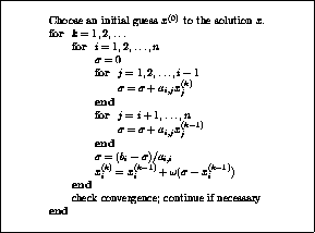
Figure: The SOR Method
Jack Dongarra
Mon Nov 20 08:52:54 EST 1995
Choosing the Value of <IMG ALIGN=BOTTOM SRC="http://www.netlib.org/utk/papers/templates/_22900_tex2html_wrap4973.gif">
Next:
The Symmetric Successive
Up:
The Successive Overrelaxation
Previous:
The Successive Overrelaxation
If  , the SOR method simplifies
to the Gauss-Seidel method. A theorem due to
Kahan
[130] shows that SOR fails to
converge if
is outside the interval
, the SOR method simplifies
to the Gauss-Seidel method. A theorem due to
Kahan
[130] shows that SOR fails to
converge if
is outside the interval  . Though
technically the term underrelaxation
should be used when
. Though
technically the term underrelaxation
should be used when  , for convenience the term
overrelaxation
is now used for any value
of
, for convenience the term
overrelaxation
is now used for any value
of  .
.
In general, it is not possible to compute in advance the value
of
that is optimal with respect to the rate of convergence of
SOR. Even when it is possible to compute the optimal value
for
, the expense of such computation is usually prohibitive.
Frequently, some heuristic estimate is used, such as  where
is the mesh spacing of the discretization of the
underlying physical domain.
where
is the mesh spacing of the discretization of the
underlying physical domain.
If the coefficient matrix
is symmetric and positive definite, the
SOR iteration is guaranteed to converge for any
value of
between 0 and 2, though the choice of
can
significantly affect the rate at which the SOR iteration
converges. Sophisticated implementations of the SOR
algorithm (such as that found in ITPACK
[140]) employ adaptive
parameter estimation schemes to try to home in on the appropriate
value of
by estimating the rate at which the iteration is
converging.
Adaptive methods: Iterative methods that collect information
about the coefficient matrix during the iteration process, and use
this to speed up convergence.
Symmetric matrix: See: Matrix properties.
Diagonally dominant matrix: See: Matrix properties
-Matrix: See: Matrix properties.
Positive definite matrix: See: Matrix properties.
Matrix properties: We call a square matrix
- Symmetric
- if
for all
,
.
- Positive definite
- if it satisfies
for all nonzero vectors
.
- Diagonally dominant
- if
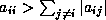 .
.
- An
-matrix
- if
for
, and it
is nonsingular with
for all
,
.
For coefficient matrices of a special class called consistently
ordered with property A (see
Young
[217]), which includes certain orderings of matrices
arising from the discretization of elliptic PDEs, there is a direct
relationship between the spectra of the Jacobi
and SOR iteration matrices. In principle, given the
spectral radius  of the
Jacobi iteration matrix, one can determine a priori the theoretically optimal value of
for SOR:
of the
Jacobi iteration matrix, one can determine a priori the theoretically optimal value of
for SOR:

This is seldom done, since calculating the spectral radius of the
Jacobi matrix requires an impractical amount of computation. However,
relatively inexpensive rough estimates of
(for example, from
the power method, see Golub and Van Loan [p. 351]GoVL:matcomp)
can yield reasonable estimates for the optimal value of
.
Next:
The Symmetric Successive
Up:
The Successive Overrelaxation
Previous:
The Successive Overrelaxation
Jack Dongarra
Mon Nov 20 08:52:54 EST 1995
The Symmetric Successive Overrelaxation Method
Next:
Notes and References
Up:
Stationary Iterative Methods
Previous:
Choosing the Value
If we assume that the coefficient matrix
is symmetric, then the
Symmetric Successive Overrelaxation method, or SSOR, combines two SOR
sweeps together in such a way that the resulting iteration matrix is
similar to a symmetric matrix. Specifically, the
first SOR sweep is carried out as
in (
), but in the second sweep the unknowns are
updated in the reverse order. That is, SSOR is a forward
SOR sweep followed by a
backward SOR sweep. The
similarity of the SSOR iteration matrix to a symmetric
matrix permits the application of SSOR as a preconditioner
for other iterative schemes for symmetric matrices. Indeed, this is
the primary motivation for SSOR since its convergence
rate
, with an optimal value of
, is
usually slower than the convergence rate of SOR with
optimal
(see Young [page 462]Yo:book). For details on
using SSOR as a preconditioner, see
Chapter
.
In matrix terms, the SSOR iteration can be expressed as
follows:

where

and

Note that  is simply the iteration matrix for SOR
from (
), and that
is simply the iteration matrix for SOR
from (
), and that  is the same, but with the
roles of
and
reversed.
is the same, but with the
roles of
and
reversed.
The pseudocode for the SSOR algorithm is given in
Figure
.
Figure: The SSOR Method
Jack Dongarra
Mon Nov 20 08:52:54 EST 1995
Notes and References
Next:
Nonstationary Iterative Methods
Up:
Stationary Iterative Methods
Previous:
The Symmetric Successive
The modern treatment of iterative methods dates back to the
relaxation
method of Southwell
[193].
This was the precursor to the SOR method, though the order in which
approximations to the unknowns were relaxed varied during the
computation. Specifically, the next unknown was chosen based upon
estimates of the location of the largest error in the current
approximation. Because of this, Southwell's relaxation method was
considered impractical for automated computing. It is interesting to
note that the introduction of multiple-instruction, multiple
data-stream (MIMD) parallel computers has rekindled an interest in
so-called asynchronous
, or chaotic
iterative methods (see Chazan and
Miranker
[54], Baudet
[30], and
Elkin
[92]), which are closely related to Southwell's
original relaxation method. In chaotic methods, the order of
relaxation is unconstrained, thereby eliminating costly
synchronization of the processors, though the effect on convergence is
difficult to predict.
The notion of accelerating the convergence of an iterative method by
extrapolation predates the development of SOR. Indeed, Southwell used
overrelaxation to accelerate the convergence of
his original relaxation method
. More
recently, the ad hoc SOR
method, in
which a different relaxation factor
is used for updating each
variable, has given impressive results for some classes of
problems (see Ehrlich
[83]).
The three main references for the theory of stationary iterative
methods are Varga
[211], Young
[217] and Hageman and
Young
[120]. The reader is referred to these books (and
the references therein) for further details concerning the methods
described in this section.
Jack Dongarra
Mon Nov 20 08:52:54 EST 1995
Nonstationary Iterative Methods
Next:
Conjugate Gradient Method
Up:
Iterative Methods
Previous:
Notes and References
Nonstationary methods differ from stationary methods in that the
computations involve information that changes at each iteration.
Typically, constants are computed by taking inner products of
residuals or other vectors arising from the iterative method.
Jack Dongarra
Mon Nov 20 08:52:54 EST 1995
Author's Affiliations
Next:
Acknowledgments
Up:
Templates for the Solution
Previous:
How to Use
-
-
Richard Barrett
Los Alamos National Laboratory
-
-
Michael Berry
University of Tennessee, Knoxville
-
-
Tony Chan
University of California, Los Angeles
-
-
James Demmel
University of California, Berkeley
-
-
June Donato
Oak Ridge National Laboratory
-
-
Jack Dongarra
University of Tennessee, Knoxville
and Oak Ridge National Laboratory
-
-
Victor Eijkhout
University of California, Los Angeles
-
-
Roldan Pozo
National Institute of Standards and Technology
-
-
Charles Romine
Oak Ridge National Laboratory
-
-
Henk van der Vorst
Utrecht University, the Netherlands
Jack Dongarra
Mon Nov 20 08:52:54 EST 1995
Conjugate Gradient Method (CG)
Next:
Theory
Up:
Nonstationary Iterative Methods
Previous:
Nonstationary Iterative Methods
The Conjugate Gradient method is
an effective method for symmetric positive definite systems. It is
the oldest and best known of the nonstationary methods discussed
here. The method proceeds by generating vector sequences of iterates
(i.e., successive approximations to the solution), residuals
corresponding to the iterates, and search directions
used in updating
the iterates and residuals. Although the length of these sequences can
become large, only a small number of vectors needs to be kept in
memory. In every iteration of the method, two inner products are
performed in order to compute update scalars that are defined to
make the sequences satisfy certain orthogonality conditions. On a
symmetric positive definite linear system these conditions imply that
the distance to the true solution is minimized in some norm.
The iterates
are updated in each iteration by a multiple
 of the
search direction vector
:
of the
search direction vector
:

Correspondingly the residuals  are updated as

The choice  minimizes
  over all possible choices for
  in
equation (
).
in
equation (
).
The search directions are updated using the residuals

where the choice  ensures
that
and
ensures
that
and  - or equivalently,
 and
and  - are orthogonal
. In fact, one can
show that this choice of
- are orthogonal
. In fact, one can
show that this choice of  makes
and
orthogonal to
all previous
makes
and
orthogonal to
all previous  and
and  respectively.
The pseudocode for the Preconditioned Conjugate Gradient Method is
given in Figure
. It uses a preconditioner
;
for  one obtains the unpreconditioned version of the Conjugate Gradient
Algorithm. In that case the algorithm may be further simplified by skipping
the ``solve'' line, and replacing
one obtains the unpreconditioned version of the Conjugate Gradient
Algorithm. In that case the algorithm may be further simplified by skipping
the ``solve'' line, and replacing  by
(and
by
(and  by
by  ).
).
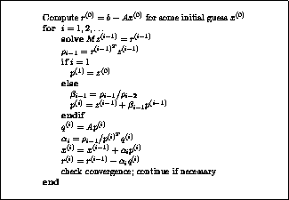
Figure: The Preconditioned Conjugate Gradient Method
Jack Dongarra
Mon Nov 20 08:52:54 EST 1995
Theory
Next:
Convergence
Up:
Conjugate Gradient Method
Previous:
Conjugate Gradient Method
The unpreconditioned conjugate gradient method constructs the
th
iterate
as an element of
 so that
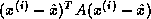 is minimized
, where
is the exact solution of
. This minimum is guaranteed
to exist in general only if
is symmetric positive definite. The
preconditioned version of the method uses a different subspace for
constructing the iterates, but it satisfies the same minimization
property, although over this different subspace. It requires in
addition that the preconditioner
is symmetric and positive
definite.
is minimized
, where
is the exact solution of
. This minimum is guaranteed
to exist in general only if
is symmetric positive definite. The
preconditioned version of the method uses a different subspace for
constructing the iterates, but it satisfies the same minimization
property, although over this different subspace. It requires in
addition that the preconditioner
is symmetric and positive
definite.
The above minimization of the error is equivalent to the residuals
being  orthogonal (that is,
 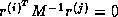 if
). Since for symmetric
an orthogonal basis for the Krylov subspace
if
). Since for symmetric
an orthogonal basis for the Krylov subspace
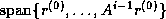 can be
constructed with only three-term recurrences
, such a recurrence also
suffices for generating the residuals. In the Conjugate
Gradient method two coupled two-term recurrences are used; one that
updates residuals using a search direction vector, and one updating
the search direction
with a newly computed residual.
This makes the
Conjugate Gradient Method quite attractive computationally.
can be
constructed with only three-term recurrences
, such a recurrence also
suffices for generating the residuals. In the Conjugate
Gradient method two coupled two-term recurrences are used; one that
updates residuals using a search direction vector, and one updating
the search direction
with a newly computed residual.
This makes the
Conjugate Gradient Method quite attractive computationally.
Krylov sequence: For a given matrix
and vector
, the
sequence of vectors
, or a finite initial part
of this sequence.
Krylov subspace: The subspace spanned by a Krylov sequence.
There is a close relationship between the Conjugate Gradient method
and the Lanczos method
for determining eigensystems, since both are
based on the construction of an orthogonal basis for the Krylov
subspace, and a similarity transformation of the coefficient matrix to
tridiagonal form. The coefficients computed during
the CG iteration then arise from the
factorization of this
tridiagonal matrix.
From the CG iteration one can reconstruct the Lanczos process, and vice versa;
see Paige and Saunders
[168]
and Golub and Van Loan [.2.6]GoVL:matcomp.
This relationship can be exploited to obtain relevant information
about the eigensystem of the (preconditioned) matrix
;
see §
.
Next:
Convergence
Up:
Conjugate Gradient Method
Previous:
Conjugate Gradient Method
Jack Dongarra
Mon Nov 20 08:52:54 EST 1995
Convergence
Next:
Implementation
Up:
Conjugate Gradient Method
Previous:
Theory
Accurate predictions of the convergence of iterative methods are
difficult to make, but useful bounds can often be obtained. For the
Conjugate Gradient method, the error can be
bounded in terms of the spectral condition number  of the
matrix
of the
matrix  . (Recall that if
and
are the largest and smallest eigenvalues of a
symmetric positive definite matrix
, then the spectral condition
number of
is
. (Recall that if
and
are the largest and smallest eigenvalues of a
symmetric positive definite matrix
, then the spectral condition
number of
is  . If
is the exact solution of the linear system
,
with symmetric positive definite matrix
, then for CG
with
symmetric positive definite preconditioner
, it can be shown that
. If
is the exact solution of the linear system
,
with symmetric positive definite matrix
, then for CG
with
symmetric positive definite preconditioner
, it can be shown that

where 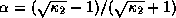 (see Golub and Van Loan
[][.2.8]GoVL:matcomp, and
Kaniel
[131]), and
(see Golub and Van Loan
[][.2.8]GoVL:matcomp, and
Kaniel
[131]), and
 . From this
relation we see that the number of iterations to reach a relative
reduction of
. From this
relation we see that the number of iterations to reach a relative
reduction of  in the error is proportional
to
in the error is proportional
to  .
.
In some cases, practical application of the above error bound is
straightforward. For example, elliptic second order partial
differential equations typically give rise to coefficient matrices
with  (where
is the discretization mesh
width), independent of the order of the finite elements or differences
used, and of the number of space dimensions of the problem (see for
instance Axelsson and Barker [.5]AxBa:febook). Thus,
without preconditioning, we expect a number of iterations proportional
to
(where
is the discretization mesh
width), independent of the order of the finite elements or differences
used, and of the number of space dimensions of the problem (see for
instance Axelsson and Barker [.5]AxBa:febook). Thus,
without preconditioning, we expect a number of iterations proportional
to  for the Conjugate Gradient method.
Other results concerning the behavior of the Conjugate Gradient
algorithm have been obtained. If the extremal eigenvalues of the
matrix
are well separated, then one often observes so-called
(see Concus, Golub and
O'Leary
[58]); that is, convergence at a
rate that increases per iteration.
This phenomenon is explained by
the fact that CG tends to eliminate components of the error in the
direction of eigenvectors associated with extremal eigenvalues first.
After these have been eliminated, the method proceeds as if these
eigenvalues did not exist in the given system, i.e., the
convergence rate depends on a reduced system with a (much) smaller
condition number (for an analysis of this, see Van der Sluis and
Van der Vorst
[199]). The effectiveness of
the preconditioner in reducing the condition number and in separating
extremal eigenvalues can be deduced by studying the approximated
eigenvalues of the related Lanczos process.
Next:
Implementation
Up:
Conjugate Gradient Method
Previous:
Theory
Jack Dongarra
Mon Nov 20 08:52:54 EST 1995
Implementation
Next:
Further references
Up:
Conjugate Gradient Method
Previous:
Convergence
The Conjugate Gradient method involves one matrix-vector product, three
vector updates, and two inner products per iteration. Some slight
computational variants exist that have the same
structure (see Reid
[179]). Variants that cluster the inner products
, a favorable property on
parallel machines, are discussed in §
.
For a discussion of the Conjugate Gradient method
on vector and shared
memory computers, see Dongarra, et
al.
[166]
[71]. For discussions
of the method for more general parallel architectures
see Demmel, Heath and Van der Vorst
[67] and
Ortega
[166], and the references therein.
Jack Dongarra
Mon Nov 20 08:52:54 EST 1995
Further references
Next:
MINRES and SYMMLQ
Up:
Conjugate Gradient Method
Previous:
Implementation
A more formal presentation of CG, as well as many theoretical
properties, can be found in the textbook by Hackbusch
[118].
Shorter presentations are given in Axelsson and Barker
[14]
and Golub and Van Loan
[109]. An overview of papers
published in the first 25 years of existence of the method is given
in Golub and O'Leary
[108].
Jack Dongarra
Mon Nov 20 08:52:54 EST 1995
MINRES and SYMMLQ
Next:
Theory
Up:
Nonstationary Iterative Methods
Previous:
Further references
The Conjugate Gradient method can be viewed as a special variant of
the Lanczos method
(see §
) for positive definite
symmetric systems. The MINRES
and SYMMLQ
methods are variants that can
be applied to symmetric indefinite systems.
The vector sequences in the Conjugate Gradient method
correspond to a
factorization of a tridiagonal matrix similar to the coefficient
matrix. Therefore, a breakdown
of the algorithm can occur
corresponding to a zero pivot if the matrix is indefinite.
Furthermore, for indefinite matrices the minimization property of the
Conjugate Gradient method
is no longer well-defined. The
MINRES
and SYMMLQ
methods are variants of the CG method that avoid the
-factorization and do not suffer from breakdown. MINRES
minimizes
the residual in the
-norm
. SYMMLQ solves the projected
system, but
does not minimize anything (it keeps the residual orthogonal to all
previous ones
). The convergence
behavior of Conjugate Gradients and MINRES
for indefinite systems was
analyzed by Paige, Parlett, and Van der Vorst
[167].
Breakdown: The occurrence of a zero coefficient that is
to be used as a divisor in an iterative method.
Jack Dongarra
Mon Nov 20 08:52:54 EST 1995
Theory
Next:
CG on the
Up:
MINRES and SYMMLQ
Previous:
MINRES and SYMMLQ
When
is not positive definite, but symmetric, we can still
construct an orthogonal basis for the Krylov subspace
by three term recurrence relations.
Eliminating the
search directions
in equations (
)
and (
) gives a recurrence

which can be written in matrix form as

where  is an
is an  tridiagonal matrix
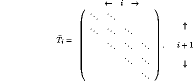
In this case we have the problem that  no
longer defines an inner product. However we can still try to minimize
the residual in the
-norm by obtaining
no
longer defines an inner product. However we can still try to minimize
the residual in the
-norm by obtaining

that minimizes

Now we exploit the fact that if  , then
 is an orthonormal transformation with respect to
the current Krylov subspace:
is an orthonormal transformation with respect to
the current Krylov subspace:

and this final expression can simply be seen as a minimum norm least
squares problem.
The element in the  position of
can be
annihilated by a simple Givens rotation and the resulting upper
bidiagonal system (the other subdiagonal elements having been removed
in previous iteration steps) can simply be solved, which leads to the
MINRES method (see Paige and Saunders
[168]).
position of
can be
annihilated by a simple Givens rotation and the resulting upper
bidiagonal system (the other subdiagonal elements having been removed
in previous iteration steps) can simply be solved, which leads to the
MINRES method (see Paige and Saunders
[168]).
Another possibility is to solve the system
 , as in the CG method (
 is the upper
 part of
). Other than in CG we cannot rely on
the existence of a Cholesky decomposition
(since
is not positive
definite). An alternative is then to decompose
by an
-decomposition. This again leads to simple recurrences and the
resulting method is known as SYMMLQ (see Paige and Saunders
[168]).
part of
). Other than in CG we cannot rely on
the existence of a Cholesky decomposition
(since
is not positive
definite). An alternative is then to decompose
by an
-decomposition. This again leads to simple recurrences and the
resulting method is known as SYMMLQ (see Paige and Saunders
[168]).
Jack Dongarra
Mon Nov 20 08:52:54 EST 1995
CG on the Normal Equations, CGNE and CGNR
Next:
Theory
Up:
Nonstationary Iterative Methods
Previous:
Theory
The CGNE
and CGNR methods
are the simplest methods for nonsymmetric or
indefinite systems. Since other methods for such systems are in
general rather more complicated than the Conjugate Gradient method,
transforming the system to a symmetric definite one and then applying
the Conjugate Gradient method is attractive for its coding simplicity.
Jack Dongarra
Mon Nov 20 08:52:54 EST 1995
Theory
Next:
Generalized Minimal Residual
Up:
CG on the
Previous:
CG on the
If a system of linear equations
has a nonsymmetric, possibly
indefinite (but nonsingular), coefficient matrix, one obvious attempt
at a solution is to apply Conjugate Gradient to a related symmetric positive definite system,
. While
this approach is easy to understand and code, the convergence speed of
the Conjugate Gradient method now depends on the square of the
condition number of the original coefficient matrix. Thus the
rate of convergence of the CG procedure on the normal equations
may be slow.
Several proposals have been made to improve the numerical stability of
this method. The best known is by Paige and Saunders
[169]
and is based upon applying the Lanczos method
to the auxiliary system
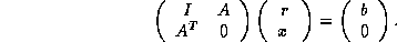
A clever execution of this scheme delivers the factors
and
of the
-decomposition of the tridiagonal matrix that would
have been computed by carrying out the Lanczos procedure with
.
Another means for improving the numerical stability of this normal
equations approach is suggested by Björck and Elfving in
[34].
The observation that the matrix
is used in the construction of
the iteration coefficients through an inner product like  leads to the suggestion that such an inner product
be replaced by
leads to the suggestion that such an inner product
be replaced by  .
.
Jack Dongarra
Mon Nov 20 08:52:54 EST 1995
Generalized Minimal Residual (GMRES)
Next:
Theory
Up:
Nonstationary Iterative Methods
Previous:
Theory
The Generalized Minimal Residual method
[189]
is an extension of MINRES
(which is only applicable to symmetric systems) to unsymmetric
systems. Like MINRES, it generates a sequence of orthogonal vectors,
but in the absence of symmetry this can no longer be done with short
recurrences; instead, all previously computed vectors in the
orthogonal sequence have to be retained. For this reason,
``restarted
'' versions of the method are used.
In the Conjugate Gradient method, the residuals form an orthogonal
basis
for the space  . In GMRES, this
basis is formed explicitly:
. In GMRES, this
basis is formed explicitly:
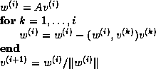
The reader may recognize this as a modified Gram-Schmidt
orthogonalization.
Applied to the Krylov
sequence
 this orthogonalization
is called the ``Arnoldi method''
[6].
The inner product coefficients
this orthogonalization
is called the ``Arnoldi method''
[6].
The inner product coefficients  and
and
 are stored in an upper Hessenberg matrix.
The GMRES iterates are constructed as

where the coefficients  have been chosen to minimize the residual
norm
have been chosen to minimize the residual
norm  . The GMRES algorithm has the property that this
residual norm can be computed without the iterate having been formed.
Thus, the expensive action of forming the iterate can be postponed
until the residual norm is deemed small enough.
. The GMRES algorithm has the property that this
residual norm can be computed without the iterate having been formed.
Thus, the expensive action of forming the iterate can be postponed
until the residual norm is deemed small enough.
The pseudocode for the restarted
GMRES(
) algorithm with preconditioner
is given in
Figure
.
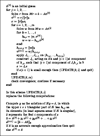
Figure: The Preconditioned GMRES Method
Jack Dongarra
Mon Nov 20 08:52:54 EST 1995
Acknowledgments
Next:
Contents
Up:
Templates for the Solution
Previous:
Author's Affiliations
The authors gratefully acknowledge the valuable assistance of many
people who commented on preliminary drafts of this book. In
particular, we thank Loyce Adams, Bill Coughran,
Matthew Fishler, Peter Forsyth,
Roland Freund, Gene
Golub, Eric Grosse, Mark Jones, David Kincaid, Steve Lee, Tarek
Mathew, Noël Nachtigal, Jim Ortega, and David Young for their
insightful comments. We also thank Geoffrey Fox for initial
discussions on the concept of templates, and Karin Remington for
designing the front cover.
This work was supported in part by DARPA and ARO under contract number
DAAL03-91-C-0047, the National Science Foundation Science and
Technology Center Cooperative Agreement No. CCR-8809615, the Applied
Mathematical Sciences subprogram of the Office of Energy Research,
U.S. Department of Energy, under Contract DE-AC05-84OR21400, and the
Stichting Nationale Computer Faciliteit (NCF) by Grant CRG 92.03.
Jack Dongarra
Mon Nov 20 08:52:54 EST 1995
Theory
Next:
Implementation
Up:
Generalized Minimal Residual
Previous:
Generalized Minimal Residual
The Generalized Minimum
Residual (GMRES) method
is designed to solve nonsymmetric linear
systems (see Saad and Schultz
[189]). The most popular
form of GMRES is based on the modified Gram-Schmidt procedure, and
uses restarts
to control storage requirements.
If no restarts are used, GMRES
(like any orthogonalizing Krylov-subspace method) will
converge in no more than
steps (assuming exact arithmetic). Of
course this is of no practical value when
is large; moreover, the
storage and computational requirements in the absence of restarts are
prohibitive. Indeed, the crucial element for successful application
of GMRES(
) revolves around the decision of when to restart; that
is, the choice of
. Unfortunately, there exist examples for which
the method stagnates
and convergence takes place only
at the
th step. For such systems, any choice of
less than
fails to converge.
Saad and Schultz
[189] have proven several useful results.
In particular, they show that if the coefficient matrix
is real
and nearly positive definite, then a ``reasonable'' value for
may be selected. Implications of the choice of
are discussed
below.
Jack Dongarra
Mon Nov 20 08:52:54 EST 1995
Implementation
Next:
BiConjugate Gradient (BiCG)
Up:
Generalized Minimal Residual
Previous:
Theory
A common implementation of GMRES
is suggested by Saad and Schultz in
[189] and
relies on using modified Gram-Schmidt orthogonalization. Householder
transformations, which are relatively costly but stable, have also
been proposed. The Householder approach results in a three-fold
increase in work associated with inner products and
vector updates (not with matrix vector products);
however, convergence may be better, especially for
ill-conditioned systems
(see Walker
[214]). From
the point of view of parallelism
, Gram-Schmidt orthogonalization may be
preferred, giving up some stability for better parallelization
properties (see Demmel, Heath and Van der Vorst
[67]).
Here we adopt the Modified Gram-Schmidt approach.
The major drawback to GMRES is that the amount of work and storage
required per iteration rises linearly with the iteration count.
Unless one is fortunate enough to obtain extremely fast convergence,
the cost will rapidly become prohibitive. The usual way to overcome
this limitation is by restarting
the iteration. After a chosen number
(
) of iterations, the accumulated data are cleared and the
intermediate results are used as the initial data for the next
iterations. This procedure is repeated until convergence is
achieved. The difficulty is in choosing an appropriate value for
.
If
is ``too small'', GMRES(
) may be slow to converge, or fail
to converge entirely. A value of
that is larger than necessary
involves excessive work (and uses more storage). Unfortunately, there
are no definite rules governing the choice of
-choosing when to
restart is a matter of experience.
For a discussion of GMRES for vector and shared memory computers see
Dongarra et al.
[71]; for more general
architectures,
see Demmel, Heath and Van der Vorst
[67]
.
Jack Dongarra
Mon Nov 20 08:52:54 EST 1995
BiConjugate Gradient (BiCG)
Next:
Convergence
Up:
Nonstationary Iterative Methods
Previous:
Implementation
The Conjugate Gradient method is not suitable for nonsymmetric systems
because the residual vectors cannot be made orthogonal with short
recurrences (for proof of this see Voevodin
[213] or Faber and
Manteuffel
[96]). The GMRES method retains
orthogonality of the residuals by using long recurrences, at the cost
of a larger storage demand. The BiConjugate Gradient method takes
another approach, replacing the orthogonal sequence of residuals by
two mutually orthogonal sequences, at the price of no longer providing
a minimization.
The update relations for residuals in the Conjugate Gradient method
are augmented in the BiConjugate Gradient method by relations
that are similar
but based on
instead of
. Thus we update two sequences of
residuals

and two sequences of search directions

The choices
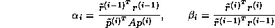
ensure the bi-orthogonality
relations

The pseudocode for the Preconditioned BiConjugate Gradient
Method with preconditioner
is given in Figure
.
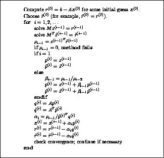
Figure: The Preconditioned BiConjugate Gradient Method
Jack Dongarra
Mon Nov 20 08:52:54 EST 1995
Convergence
Next:
Implementation
Up:
BiConjugate Gradient (BiCG)
Previous:
BiConjugate Gradient (BiCG)
Few theoretical results are known about the convergence of BiCG. For
symmetric positive definite systems the method delivers the same
results as CG, but at twice the cost per iteration. For nonsymmetric
matrices it has been shown that in phases of the process where there
is significant reduction of the norm of the residual, the method is
more or less comparable to full GMRES
(in terms of numbers of
iterations) (see Freund and Nachtigal
[102]). In practice
this is often confirmed, but
it is also observed that the convergence behavior may be quite
irregular
, and the method may even break
down
. The breakdown
situation due to the possible event that
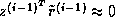 can be circumvented by so-called
look-ahead strategies
(see Parlett, Taylor and Liu
[172]). This
leads to
complicated codes and is beyond the scope of this book. The other
breakdown
situation,
can be circumvented by so-called
look-ahead strategies
(see Parlett, Taylor and Liu
[172]). This
leads to
complicated codes and is beyond the scope of this book. The other
breakdown
situation,  ,
occurs when the
-decomposition fails (see the theory subsection
of §
), and can be repaired by
using another decomposition. This is done in the version of QMR
that we adopted
(see §
).
,
occurs when the
-decomposition fails (see the theory subsection
of §
), and can be repaired by
using another decomposition. This is done in the version of QMR
that we adopted
(see §
).
Sometimes, breakdown
or near-breakdown situations can be
satisfactorily avoided by a restart
at the iteration step immediately
before the (near-) breakdown step. Another possibility is to switch to
a more robust (but possibly more expensive) method, like GMRES.
Jack Dongarra
Mon Nov 20 08:52:54 EST 1995
Implementation
Next:
Quasi-Minimal Residual (QMR)
Up:
BiConjugate Gradient (BiCG)
Previous:
Convergence
BiCG requires computing a matrix-vector product  and a
transpose product
and a
transpose product  . In some applications the
latter product may be impossible to perform, for instance if the
matrix is not formed explicitly
and the regular product is only given in operation form, for instance
as a function call evaluation.
. In some applications the
latter product may be impossible to perform, for instance if the
matrix is not formed explicitly
and the regular product is only given in operation form, for instance
as a function call evaluation.
In a parallel environment
, the two matrix-vector products can
theoretically be performed simultaneously; however,
in a distributed-memory environment, there will be extra communication
costs associated with one of the two matrix-vector products, depending
upon the storage scheme for
.
A duplicate copy of the
matrix will alleviate this problem, at the cost of doubling the
storage requirements for the matrix.
Care must also be exercised in choosing the preconditioner, since
similar problems arise during the two solves involving the
preconditioning matrix.
It is difficult to make a fair comparison between GMRES
and BiCG.
GMRES really minimizes a residual, but at the cost of increasing work
for keeping all residuals orthogonal and increasing demands for memory
space. BiCG does not minimize a residual, but often its
accuracy is comparable to GMRES, at the cost of twice the amount of matrix
vector products per iteration step. However, the generation of the
basis vectors is relatively cheap and the memory requirements are
modest. Several variants of BiCG have been proposed that increase
the effectiveness of this class of methods in certain circumstances. These
variants (CGS and Bi-CGSTAB) will be discussed in coming subsections.
Jack Dongarra
Mon Nov 20 08:52:54 EST 1995
Quasi-Minimal Residual (QMR)
Next:
Convergence
Up:
Nonstationary Iterative Methods
Previous:
Implementation
The BiConjugate Gradient method often displays rather irregular
convergence
behavior. Moreover, the implicit
decomposition of the
reduced tridiagonal system may not exist, resulting in breakdown
of the algorithm. A related algorithm, the
Quasi-Minimal Residual method of Freund and
Nachtigal
[102],
[103]
attempts to overcome
these problems. The main idea behind this algorithm is to solve the
reduced tridiagonal system in a least squares sense, similar to the
approach followed in GMRES.
Since the constructed basis for the
Krylov subspace
is bi-orthogonal
, rather than orthogonal as in GMRES,
the obtained solution is viewed as a quasi-minimal residual solution,
which explains the name. Additionally, QMR uses look-ahead techniques
to avoid breakdowns in the underlying Lanczos process, which makes it
more robust than BiCG.
Figure: The Preconditioned Quasi Minimal Residual Method
without Look-ahead
Jack Dongarra
Mon Nov 20 08:52:54 EST 1995
Convergence
Next:
Implementation
Up:
Quasi-Minimal Residual (QMR)
Previous:
Quasi-Minimal Residual (QMR)
The convergence behavior of QMR
is typically much smoother than for BiCG.
Freund and Nachtigal
[102] present quite general error
bounds which show that
QMR may be expected to converge about as fast as GMRES. From a relation
between the residuals in BiCG and QMR
(Freund and Nachtigal [relation (5.10)]FrNa:qmr) one may deduce
that at phases in the
iteration process where BiCG makes significant progress, QMR has arrived
at about the same approximation for
.
On the other hand, when BiCG makes
no progress at all
, QMR may still show slow convergence.
The look-ahead steps in the version of the QMR method
discussed in
[102] prevents breakdown in all cases
but the so-called ``incurable breakdown'', where no practical number of
look-ahead steps would yield a next iterate.
Jack Dongarra
Mon Nov 20 08:52:54 EST 1995
Implementation
Next:
Conjugate Gradient Squared
Up:
Quasi-Minimal Residual (QMR)
Previous:
Convergence
The pseudocode for the Preconditioned Quasi Minimal Residual
Method, with preconditioner  ,
is given in Figure
.
This algorithm follows the two term recurrence
version
without look-ahead, presented by Freund and
Nachtigal
[103] as Algorithm 7.1.
This version of QMR is simpler to implement than the full QMR method
with look-ahead, but it is susceptible to breakdown of the underlying
Lanczos process. (Other implementational variations are whether to
scale Lanczos vectors or not, or to use three-term recurrences instead
of coupled two-term recurrences. Such decisions usually have implications
for the stability and the efficiency of the algorithm.)
A professional implementation of QMR
with look-ahead is given in Freund and Nachtigal's QMRPACK, which
is available through netlib; see Appendix
.
,
is given in Figure
.
This algorithm follows the two term recurrence
version
without look-ahead, presented by Freund and
Nachtigal
[103] as Algorithm 7.1.
This version of QMR is simpler to implement than the full QMR method
with look-ahead, but it is susceptible to breakdown of the underlying
Lanczos process. (Other implementational variations are whether to
scale Lanczos vectors or not, or to use three-term recurrences instead
of coupled two-term recurrences. Such decisions usually have implications
for the stability and the efficiency of the algorithm.)
A professional implementation of QMR
with look-ahead is given in Freund and Nachtigal's QMRPACK, which
is available through netlib; see Appendix
.
We have modified Algorithm 7.1 in
[103] to include a
relatively inexpensive recurrence relation for the computation
of the residual vector. This requires a few extra vectors of storage
and vector update operations per iteration, but it avoids expending
a matrix-vector product on the residual calculation.
Also, the algorithm has been modified so that only two
full preconditioning steps are required instead of three.
Computation of the residual is done for the convergence test.
If one uses right (or post) preconditioning, that is  , then a
cheap upper bound for
, then a
cheap upper bound for  can be computed in each iteration,
avoiding the recursions for
. For details,
see Freund and Nachtigal [proposition 4.1]FrNa:qmr. This upper
bound may be
pessimistic by a factor of at most
can be computed in each iteration,
avoiding the recursions for
. For details,
see Freund and Nachtigal [proposition 4.1]FrNa:qmr. This upper
bound may be
pessimistic by a factor of at most  .
.
QMR has roughly the same problems with respect to vector and parallel
implementation as BiCG. The scalar overhead per iteration is slightly
more than for BiCG. In all cases where the slightly cheaper BiCG method
converges irregularly
(but fast enough),
QMR may be preferred for stability reasons.
Jack Dongarra
Mon Nov 20 08:52:54 EST 1995
Conjugate Gradient Squared Method (CGS)
Next:
Convergence
Up:
Nonstationary Iterative Methods
Previous:
Implementation
In BiCG, the residual vector
can be regarded as
the product
of
and an
th degree polynomial in
, that is

This same polynomial satisfies
 so that

This suggests that if  reduces
to a smaller
vector
, then it might be advantageous to apply this
``contraction'' operator twice, and compute
reduces
to a smaller
vector
, then it might be advantageous to apply this
``contraction'' operator twice, and compute  .
Equation (
) shows that the iteration coefficients can
still be recovered from these vectors, and it turns out to be easy to
find the corresponding approximations for
. This
approach leads to the Conjugate Gradient Squared method (see
Sonneveld
[192]).
.
Equation (
) shows that the iteration coefficients can
still be recovered from these vectors, and it turns out to be easy to
find the corresponding approximations for
. This
approach leads to the Conjugate Gradient Squared method (see
Sonneveld
[192]).

Figure: The Preconditioned Conjugate Gradient Squared Method
Jack Dongarra
Mon Nov 20 08:52:54 EST 1995
Convergence
Next:
Implementation
Up:
Conjugate Gradient Squared
Previous:
Conjugate Gradient Squared
Often one observes a speed of convergence for CGS that is about twice
as fast as for BiCG, which is in agreement with the observation that
the same ``contraction'' operator is applied twice. However, there is
no reason that the ``contraction'' operator, even if it really reduces
the initial residual
, should also reduce the once reduced
vector  . This is evidenced by the often
highly irregular convergence behavior of CGS
. One should be aware of
the fact that local corrections to the current solution may be so
large that cancelation effects occur. This may lead to a less
accurate solution than suggested by the updated residual
(see Van der Vorst
[207]).
The method tends to diverge if the starting guess is close to the solution.
. This is evidenced by the often
highly irregular convergence behavior of CGS
. One should be aware of
the fact that local corrections to the current solution may be so
large that cancelation effects occur. This may lead to a less
accurate solution than suggested by the updated residual
(see Van der Vorst
[207]).
The method tends to diverge if the starting guess is close to the solution.
Jack Dongarra
Mon Nov 20 08:52:54 EST 1995
Contents
Next:
List of Figures
Up:
Templates for the Solution
Previous:
Acknowledgments
Jack Dongarra
Mon Nov 20 08:52:54 EST 1995
Implementation
Next:
BiConjugate Gradient Stabilized
Up:
Conjugate Gradient Squared
Previous:
Convergence
CGS requires about the same number of
operations per iteration as
BiCG, but does not involve computations with
. Hence, in
circumstances where computation with
is impractical, CGS may be
attractive.
The pseudocode for the Preconditioned Conjugate Gradient Squared
Method with preconditioner
is given in Figure
.
Jack Dongarra
Mon Nov 20 08:52:54 EST 1995
BiConjugate Gradient Stabilized (Bi-CGSTAB)
Next:
Convergence
Up:
Nonstationary Iterative Methods
Previous:
Implementation
The BiConjugate Gradient Stabilized method (Bi-CGSTAB) was developed to
solve nonsymmetric linear systems while avoiding the often irregular
convergence
patterns of the Conjugate
Gradient Squared
method (see Van der Vorst
[207]). Instead of computing
the CGS sequence
 , Bi-CGSTAB computes
 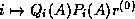 where
where  is an
th degree polynomial describing a steepest
descent update.
is an
th degree polynomial describing a steepest
descent update.
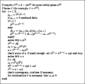
Figure: The Preconditioned BiConjugate Gradient Stabilized Method
Jack Dongarra
Mon Nov 20 08:52:54 EST 1995
Convergence
Next:
Implementation
Up:
BiConjugate Gradient Stabilized
Previous:
BiConjugate Gradient Stabilized
Bi-CGSTAB often converges about as fast as CGS,
sometimes faster and
sometimes not. CGS can be viewed as a method in which the BiCG
``contraction'' operator is applied twice. Bi-CGSTAB can be
interpreted as the product of BiCG and repeatedly applied GMRES(1). At
least locally, a residual vector is minimized
, which leads to a
considerably smoother
convergence behavior. On the
other hand, if the
local GMRES(1) step stagnates, then the Krylov subspace
is not
expanded, and Bi-CGSTAB will break down
. This is a breakdown situation
that can occur in addition to the other breakdown possibilities in the
underlying BiCG algorithm. This type of breakdown may be avoided by
combining BiCG with other methods, i.e., by selecting other
values for  (see the algorithm). One such alternative is
Bi-CGSTAB2
(see Gutknecht
[115]); more general
approaches are suggested by Sleijpen and Fokkema in
[190].
(see the algorithm). One such alternative is
Bi-CGSTAB2
(see Gutknecht
[115]); more general
approaches are suggested by Sleijpen and Fokkema in
[190].
Note that Bi-CGSTAB has two stopping tests: if the method has already
converged at the first test on the norm of
, the subsequent update
would be numerically questionable. Additionally, stopping on the first
test saves a few unnecessary operations, but this is of minor importance.
Jack Dongarra
Mon Nov 20 08:52:54 EST 1995
Implementation
Next:
Chebyshev Iteration
Up:
BiConjugate Gradient Stabilized
Previous:
Convergence
Bi-CGSTAB requires two matrix-vector products
and four inner products, i.e., two inner products more than BiCG
and CGS.
The pseudocode for the Preconditioned BiConjugate Gradient Stabilized
Method with preconditioner
is given in Figure
.
Jack Dongarra
Mon Nov 20 08:52:54 EST 1995
Chebyshev Iteration
Next:
Comparison with other
Up:
Nonstationary Iterative Methods
Previous:
Implementation
Chebyshev Iteration is another method for solving
nonsymmetric
problems (see Golub and
Van Loan [.1.5]GoVL:matcomp and
Varga [Chapter 5]Va:book).
Chebyshev Iteration avoids the computation of inner products
as is
necessary for the other nonstationary methods.
For some distributed memory architectures
these inner products are a bottleneck
with respect to efficiency. The
price one pays for avoiding inner products is that the method requires
enough knowledge about the spectrum of the coefficient matrix
that
an ellipse enveloping the spectrum can be identified
;
however this
difficulty can be overcome via an adaptive construction
developed by
Manteuffel
[146], and implemented by Ashby
[7].
Chebyshev iteration is suitable for any nonsymmetric linear system for
which the enveloping ellipse does not include the origin.
Jack Dongarra
Mon Nov 20 08:52:54 EST 1995
Comparison with other methods
Next:
Convergence
Up:
Chebyshev Iteration
Previous:
Chebyshev Iteration
Comparing the pseudocode for Chebyshev Iteration with the pseudocode
for the Conjugate Gradient method shows a high degree of similarity,
except that no inner products are computed in Chebyshev Iteration
.
Scalars
and
must be selected so that they define a family of
ellipses
with common center  and foci
  and
and  which contain the
ellipse that encloses the spectrum (or more general, field of values)
of
and for which the rate
which contain the
ellipse that encloses the spectrum (or more general, field of values)
of
and for which the rate  of
convergence is minimal:
of
convergence is minimal:

where  is the length of the
-axis of the ellipse.
is the length of the
-axis of the ellipse.
We provide code in which it is assumed that
the ellipse degenerate to the interval  ,
that is all eigenvalues are real.
For code including the adaptive determination of the iteration
parameters
and
the reader is referred
to Ashby
[7].
,
that is all eigenvalues are real.
For code including the adaptive determination of the iteration
parameters
and
the reader is referred
to Ashby
[7].
The Chebyshev
method has the advantage over GMRES that only short recurrences are
used. On the other hand, GMRES is guaranteed to generate the smallest
residual over the current search space. The BiCG methods, which also
use short recurrences, do not minimize the residual in a suitable
norm; however, unlike Chebyshev iteration, they do not require
estimation of parameters (the spectrum of
). Finally, GMRES and
BiCG may be more effective in practice, because of superlinear
convergence behavior
, which cannot be expected for
Chebyshev.
For symmetric positive definite systems the ``ellipse'' enveloping the
spectrum degenerates to the interval
on the positive
-axis, where
and
are the smallest and largest eigenvalues of
. In circumstances where the computation of inner products
is a bottleneck
, it may be advantageous to start
with CG, compute
estimates of the extremal eigenvalues from the CG coefficients, and
then after sufficient convergence of these approximations switch to
Chebyshev Iteration
. A similar strategy
may be adopted for a switch from GMRES, or BiCG-type methods, to
Chebyshev Iteration.
Next:
Convergence
Up:
Chebyshev Iteration
Previous:
Chebyshev Iteration
Jack Dongarra
Mon Nov 20 08:52:54 EST 1995
Convergence
Next:
Implementation
Up:
Chebyshev Iteration
Previous:
Comparison with other
In the symmetric case (where
and the preconditioner
are both
symmetric) for the Chebyshev Iteration we have the same upper
bound as for the Conjugate Gradient
method, provided
and
are computed from
and
(the extremal eigenvalues of the preconditioned
matrix
).
There is a severe penalty for overestimating
or underestimating the field of values. For example, if in the
symmetric case
is underestimated, then the method may
diverge; if it is overestimated then the result may be very slow
convergence. Similar statements can be made for the nonsymmetric case.
This implies that one needs fairly accurate bounds on the
spectrum of
for the method to be effective (in comparison
with CG or GMRES).
Jack Dongarra
Mon Nov 20 08:52:54 EST 1995
Implementation
Next:
Computational Aspects of
Up:
Chebyshev Iteration
Previous:
Convergence
In Chebyshev Iteration the iteration parameters
are known as soon
as one knows the ellipse containing the eigenvalues (or rather, the
field of values) of the operator. Therefore the computation of
inner products, as is necessary in methods like GMRES or CG,
is avoided
.
This avoids the synchronization points required of CG-type methods, so
machines with hierarchical or distributed memory may achieve higher
performance (it also suggests strong parallelization properties
; for a
discussion of this see Saad
[185], and Dongarra, et
al.
[71]).
Specifically, as soon as some segment of
is computed, we may begin
computing, in sequence, corresponding segments of
,
, and
.
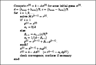
Figure: The Preconditioned Chebyshev Method
The pseudocode for the Preconditioned Chebyshev
Method with preconditioner
is given in Figure
.
It handles the case of a symmetric
positive definite coefficient matrix
. The
eigenvalues of
are assumed to be all real and in the
interval
, which does not include
zero.
Jack Dongarra
Mon Nov 20 08:52:54 EST 1995
Computational Aspects of the Methods
Next:
A short history
Up:
Iterative Methods
Previous:
Implementation
Efficient solution of a linear system is largely a function of the
proper choice of iterative method. However,
to obtain good performance, consideration must also be given to the
computational kernels of the method and how efficiently they can be
executed on the target architecture. This point is of particular
importance on parallel architectures; see §
.
Iterative methods are very different from direct methods in this
respect. The performance of direct methods, both for dense and sparse
systems, is largely that of the factorization of the matrix. This
operation is absent in iterative methods (although preconditioners may
require a setup phase), and with it, iterative methods lack dense
matrix suboperations. Since such operations can be executed at very
high efficiency on most current computer architectures, we expect a
lower flop rate for iterative than for direct methods.
(Dongarra and Van der Vorst
[74] give some
experimental results about this, and provide a benchmark code
for iterative solvers.)
Furthermore,
the basic operations in iterative methods often use indirect
addressing, depending on the data structure. Such operations also have
a relatively low efficiency of execution.
However, this lower efficiency of execution does not imply anything
about the total solution time for a given system. Furthermore,
iterative methods are usually simpler to implement than direct
methods, and since no full factorization has to be stored, they can
handle much larger systems than direct methods.
In this section we summarize for each method
- Matrix properties. Not every method will work on every problem
type, so knowledge of matrix properties is the main criterion for
selecting an iterative method.
- Computational kernels. Different methods involve different
kernels, and depending on the problem or target computer architecture
this may rule out certain methods.
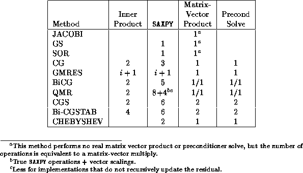
Table: Summary of Operations for Iteration
.
``a/b'' means ``a'' multiplications with the matrix and ``b'' with
its transpose.
Table
lists the storage required for each method
(without preconditioning). Note that we are not including the storage
for the original
system
and we ignore scalar storage.
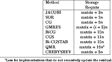
Table: Storage Requirements for the Methods in iteration
:
denotes the order of the matrix.
- Jacobi Method
- Extremely easy to use, but unless the matrix is ``strongly''
diagonally dominant, this method is probably best only considered
as an introduction to iterative methods or as a preconditioner in
a nonstationary method.
- Trivial to parallelize.
- Gauss-Seidel Method
- Typically faster convergence than Jacobi, but in general not
competitive with the nonstationary methods.
- Applicable to strictly diagonally dominant, or symmetric
positive definite matrices.
- Parallelization properties depend on structure of the
coefficient matrix. Different orderings of the unknowns have
different degrees of parallelism; multi-color orderings may give
almost full parallelism.
- This is a special case of the SOR method, obtained by
choosing
.
- Successive Over-Relaxation (SOR)
- Accelerates convergence of Gauss-Seidel (
 , over-relaxation); may yield convergence when Gauss-Seidel fails
(
, under-relaxation).
, over-relaxation); may yield convergence when Gauss-Seidel fails
(
, under-relaxation).
- Speed of convergence depends critically on
; the
optimal value for
may be estimated from the spectral
radius of the Jacobi iteration matrix under certain conditions.
- Parallelization properties are the same as those of the
Gauss-Seidel method.
- Conjugate Gradient (CG)
- Applicable to symmetric positive definite systems.
- Speed of convergence depends on the condition number; if
extremal eigenvalues are well-separated then superlinear
convergence behavior can result.
- Inner products act as synchronization points in a parallel
environment.
- Further parallel properties are largely independent of the
coefficient matrix, but depend strongly on the structure the
preconditioner.
- Generalized Minimal Residual (GMRES)
- Applicable to nonsymmetric matrices.
- GMRES leads to the smallest residual for a fixed number of
iteration steps, but these steps become increasingly expensive.
- In order to limit the increasing storage requirements and work
per iteration step, restarting is necessary. When to do so depends
on
and the right-hand side; it requires skill and experience.
- GMRES requires only matrix-vector products with the
coefficient matrix.
- The number of inner products grows linearly with the iteration
number, up to the restart point. In an implementation based on a
simple Gram-Schmidt process the inner products are independent, so
together they imply only one synchronization point. A more stable
implementation based on modified Gram-Schmidt orthogonalization
has one synchronization point per inner product.
- Biconjugate Gradient (BiCG)
- Applicable to nonsymmetric matrices.
- Requires matrix-vector products with the coefficient matrix
and its transpose. This disqualifies the method for cases where
the matrix is only given implicitly as an operator, since usually no
corresponding transpose operator is available in such cases.
- Parallelization properties are similar to those for CG; the
two matrix vector products (as well as the preconditioning steps)
are independent, so they can be done in parallel, or their
communication stages can be packaged.
- Quasi-Minimal Residual (QMR)
- Applicable to nonsymmetric matrices.
- Designed to avoid the irregular convergence behavior of BiCG,
it avoids one of the two breakdown situations of BiCG.
- If BiCG makes significant progress in one iteration step, then
QMR delivers about the same result at the same step. But when BiCG
temporarily stagnates or diverges, QMR may still further reduce
the residual, albeit very slowly.
- Computational costs per iteration are similar to BiCG, but slightly
higher. The method requires the transpose matrix-vector product.
- Parallelization properties are as for BiCG.
- Conjugate Gradient Squared (CGS)
- Applicable to nonsymmetric matrices.
- Converges (diverges) typically about twice as fast as BiCG.
- Convergence behavior is often quite irregular, which may lead
to a loss of accuracy in the updated residual.
- Computational costs per iteration are similar to BiCG, but the
method doesn't require the transpose matrix.
- Unlike BiCG, the two matrix-vector products are not
independent, so the number of synchronization points in a parallel
environment is larger.
- Biconjugate Gradient Stabilized (Bi-CGSTAB)
- Applicable to nonsymmetric matrices.
- Computational costs per iteration are similar to BiCG and CGS,
but the method doesn't require the transpose matrix.
- An alternative for CGS that avoids the irregular convergence
patterns of CGS while maintaining about the same speed of
convergence; as a result we often observe less loss of accuracy in
the updated residual.
- Chebyshev Iteration
- Applicable to nonsymmetric matrices (but presented in this
book only for the symmetric case).
- This method requires some explicit knowledge of the spectrum
(or field of values); in the symmetric case the iteration
parameters are easily obtained from the two extremal eigenvalues,
which can be estimated either directly from the matrix, or from
applying a few iterations of the Conjugate Gradient Method.
- The computational structure is similar to that of CG, but
there are no synchronization points.
- The Adaptive Chebyshev method can be used in combination with
methods as CG or GMRES, to continue the iteration once suitable
bounds on the spectrum have been obtained from these methods.
Selecting the ``best'' method for a given class of problems is largely
a matter of trial and error. It also depends on how much storage one
has available (GMRES), on the availability of
(BiCG and QMR),
and on how expensive the matrix vector products (and Solve steps with
) are in comparison to SAXPYs and inner products. If these matrix
vector products are relatively expensive, and if sufficient storage is
available then it may be attractive to use GMRES and delay restarting
as much as possible.
Table
shows the type of operations performed per
iteration. Based on the particular problem or data structure, the
user may observe that a particular operation could be performed more
efficiently.
Next:
A short history
Up:
Iterative Methods
Previous:
Implementation
Jack Dongarra
Mon Nov 20 08:52:54 EST 1995
A short history of Krylov
methods<A NAME=tex2html142 HREF="http://www.netlib.org/utk/papers/templates/footnode.html#3831">
<IMG ALIGN=BOTTOM ALT="gif" SRC="http://www.netlib.org/utk/icons/foot_motif.gif">
</A>
Next:
Survey of recent
Up:
Iterative Methods
Previous:
Computational Aspects of
Methods based on orthogonalization were developed by a number of
authors in the early '50s. Lanczos'
method
[142] was based on two mutually orthogonal
vector sequences, and his motivation came from eigenvalue problems. In
that context, the most prominent feature of the method is that it
reduces the original matrix to tridiagonal form. Lanczos
later applied his method to solving linear systems, in particular
symmetric ones
[143]. An important
property for proving convergence of the method when solving linear
systems is that the iterates are related to the initial residual by
multiplication with a polynomial in the coefficient matrix.
The joint paper by Hestenes
and Stiefel
[122], after their independent discovery
of the same method, is the classical description of the conjugate
gradient method for solving linear systems. Although error-reduction
properties are proved, and experiments showing premature convergence
are reported, the conjugate gradient method is presented here as a
direct method, rather than an iterative method.
This Hestenes/Stiefel method is closely related to a reduction of the
Lanczos method to symmetric matrices, reducing the two mutually
orthogonal sequences to one orthogonal sequence, but there is an
important algorithmic difference. Whereas Lanczos used three-term
recurrences, the method by Hestenes and Stiefel uses coupled two-term
recurrences. By combining the two two-term recurrences (eliminating
the ``search directions'') the Lanczos method is obtained.
A paper by
Arnoldi
[6] further discusses the Lanczos
biorthogonalization method, but it also presents a new method,
combining features of the Lanczos and Hestenes/Stiefel methods.
Like the Lanczos method it is applied to nonsymmetric systems, and
it does not use search directions. Like the Hestenes/Stiefel method,
it generates only one, self-orthogonal sequence. This last fact,
combined with the asymmetry of the coefficient matrix means that the
method no longer effects a reduction to tridiagonal form, but instead
one to upper Hessenberg form.
Presented as ``minimized iterations in the Galerkin method'' this
algorithm has become known as the Arnoldi algorithm.
The conjugate gradient method received little attention as a practical
method for some time, partly because of a misperceived importance of
the finite termination property. Reid
[179] pointed out that
the most important application area lay in sparse definite systems,
and this renewed the interest in the method.
Several methods have been developed in later years that employ, most
often implicitly, the upper Hessenberg matrix of the Arnoldi method.
For an overview and characterization of these orthogonal projection
methods for nonsymmetric systems
see Ashby, Manteuffel and Saylor
[10],
Saad and Schultz
[188], and Jea and
Young
[125].
Fletcher
[98] proposed an implementation of the
Lanczos method, similar to the Conjugate Gradient method, with two
coupled two-term recurrences, which he named the bi-conjugate
gradient method (BiCG).
Next:
Survey of recent
Up:
Iterative Methods
Previous:
Computational Aspects of
Jack Dongarra
Mon Nov 20 08:52:54 EST 1995
List of Figures
Next:
Introduction
Up:
Templates for the Solution
Previous:
Contents
Jack Dongarra
Mon Nov 20 08:52:54 EST 1995
Survey of recent Krylov methods
Next:
Preconditioners
Up:
Iterative Methods
Previous:
A short history
Research into the design of Krylov subspace methods for solving
nonsymmetric linear systems is an active field of research and new
methods are still emerging. In this book, we have included only the
best known and most popular methods, and in particular those for which
extensive computational experience has been gathered. In this
section, we shall briefly highlight some of the recent developments
and other methods not treated here. A survey of methods up to about
1991 can be found in Freund, Golub and
Nachtigal
[106]. Two more recent reports by
Meier-Yang
[151] and Tong
[197] have extensive
numerical comparisons among various methods, including several more
recent ones that have not been discussed in detail in this book.
Several suggestions have been made to reduce the increase in memory
and computational costs in GMRES. An obvious one is to restart (this one is included
in §
): GMRES(
). Another approach is to restrict
the GMRES search to a suitable subspace of some higher-dimensional
Krylov subspace. Methods based on this idea can be viewed as
preconditioned GMRES methods. The simplest ones exploit a fixed
polynomial preconditioner (see Johnson, Micchelli and
Paul
[126],
Saad
[183], and Nachtigal,
Reichel and Trefethen
[159]).
In more sophisticated approaches, the
polynomial preconditioner is adapted to the iterations
(Saad
[187]), or the preconditioner may even be some other
(iterative) method of choice (Van der Vorst and
Vuik
[209], Axelsson and
Vassilevski
[24]). Stagnation is prevented in the GMRESR
method (Van der Vorst and Vuik
[209]) by including
LSQR steps in some phases of the process. In De Sturler and
Fokkema
[64], part of the optimality of GMRES is
maintained in the hybrid method GCRO, in which the iterations of the
preconditioning method are kept orthogonal to the iterations of the
underlying GCR method. All these approaches have advantages for some
problems, but it is far from clear a priori which strategy is
preferable in any given case.
Recent work has focused on endowing
the BiCG method with several desirable properties:
(1) avoiding breakdown;
(2) avoiding use of the transpose;
(3) efficient use of matrix-vector products;
(4) smooth convergence; and
(5) exploiting the work expended in forming the Krylov space with
for further reduction of the residual.
As discussed before, the BiCG method can have two kinds
of breakdown: Lanczos breakdown (the underlying Lanczos
process breaks down), and pivot breakdown (the
tridiagonal matrix
implicitly generated in the
underlying Lanczos process encounters a zero pivot when
Gaussian elimination without pivoting is used to factor it).
Although such exact breakdowns are very rare in practice, near
breakdowns can cause severe numerical stability problems.
The pivot breakdown is the easier one to overcome and there have been
several approaches proposed in the literature. It should be noted
that for symmetric matrices, Lanczos breakdown cannot occur and the
only possible breakdown is pivot breakdown. The SYMMLQ and QMR
methods discussed in this book circumvent pivot breakdown by solving
least squares systems. Other methods tackling this problem can be
found
in Fletcher
[98], Saad
[181],
Gutknecht
[113], and Bank and
Chan
[29]
[28].
Lanczos breakdown is much more difficult to eliminate. Recently,
considerable attention has been given to analyzing the nature of the
Lanczos breakdown (see Parlett
[172], and
Gutknecht
[114]
[116]), as well as various look-ahead
techniques for remedying it (see Brezinski and
Sadok
[39], Brezinski, Zaglia and
Sadok
[41]
[40],
Freund and Nachtigal
[102], Parlett
[172],
Nachtigal
[160], Freund, Gutknecht and
Nachtigal
[101],
Joubert
[129], Freund, Golub
and Nachtigal
[106], and
Gutknecht
[114]
[116]). However, the resulting
algorithms are usually too complicated to give in template form (some
codes of Freund and Nachtigal are available on netlib.)
Moreover, it is still not possible to eliminate breakdowns that
require look-ahead steps of arbitrary size (incurable breakdowns). So
far, these methods have not yet received much practical use but some
form of look-ahead may prove to be a crucial component in future
methods.
In the BiCG method, the need for matrix-vector multiplies with
can be inconvenient as well as doubling the number of matrix-vector
multiplies compared with CG for each increase in the degree of the
underlying Krylov subspace.
Several recent methods have been proposed to overcome this drawback.
The most notable of these is the ingenious CGS method
by Sonneveld
[192]
discussed earlier, which computes the square of the
BiCG polynomial without requiring
- thus obviating the need for
.
When BiCG converges, CGS is often an attractive,
faster converging alternative.
However, CGS also inherits (and often magnifies) the breakdown
conditions and the irregular convergence of
BiCG (see Van der Vorst
[207]).
CGS also generated interest in the possibility of product
methods, which generate iterates corresponding to a product of the
BiCG polynomial with another polynomial of the same degree,
chosen to have certain desirable properties but
computable without recourse to
. The
Bi-CGSTAB method of Van der Vorst
[207] is such an
example, in which the auxiliary polynomial is defined by a local
minimization chosen to smooth the convergence behavior.
Gutknecht
[115] noted that Bi-CGSTAB could be viewed as a
product of BiCG and GMRES(1), and he suggested combining BiCG with
GMRES(2) for the even numbered iteration steps. This was anticipated
to lead to better convergence for the case where the eigenvalues of
are complex. A more efficient and more robust variant of this
approach has been suggested by Sleijpen and Fokkema
in
[190], where they describe how to easily combine
BiCG with any GMRES(
), for modest
.
=-1
Many other basic methods can also be squared. For example, by
squaring the Lanczos procedure, Chan, de Pillis and
Van der Vorst
[45] obtained
transpose-free implementations of BiCG and QMR. By squaring the QMR
method, Freund and Szeto
[104] derived a transpose-free
QMR squared method which is quite competitive with CGS but with much
smoother convergence. Unfortunately, these methods
require an
extra matrix-vector product per step (three instead of two) which
makes them less efficient.
In addition to Bi-CGSTAB, several recent product methods have been
designed to smooth the convergence of CGS. One idea is to use the
quasi-minimal residual (QMR) principle to obtain smoothed iterates
from the Krylov subspace generated by other product methods.
Freund
[105] proposed such a QMR version of CGS, which
he called TFQMR. Numerical experiments show that TFQMR in most
cases retains the desirable convergence features of CGS while
correcting its erratic behavior. The transpose free nature of TFQMR,
its low computational cost and its smooth convergence behavior make it
an attractive alternative to CGS. On the other hand, since the BiCG
polynomial is still used, TFQMR breaks down whenever CGS does. One
possible remedy would be to combine TFQMR with a look-ahead Lanczos
technique but this appears to be quite complicated and no methods of
this kind have yet appeared in the literature. Recently, Chan et. al.
[46] derived a similar QMR version of
Van der Vorst's Bi-CGSTAB method, which is called QMRCGSTAB. These
methods offer smoother convergence over CGS and Bi-CGSTAB with little
additional cost.
There is no clear best Krylov subspace method at this time, and there
will never be a best overall Krylov subspace method. Each of
the methods is a winner in a specific problem class, and the main
problem is to identify these classes and to construct new methods for
uncovered classes. The paper by Nachtigal, Reddy and
Trefethen
[158] shows that for any of a group of
methods (CG, BiCG, GMRES, CGNE, and CGS), there is a class of problems
for which a given method is the winner and another one is the loser.
This shows clearly that there will be no ultimate method. The best we
can hope for is some expert system that guides the user in his/her
choice. Hence, iterative methods will never reach the robustness of
direct methods, nor will they beat direct methods for all problems.
For some problems, iterative schemes will be most attractive,
and for others, direct methods (or
multigrid). We hope to find suitable methods
(and preconditioners) for classes of very large problems that we are
yet unable to solve by any known method, because of CPU-restrictions,
memory, convergence problems, ill-conditioning, et cetera.
Next:
Preconditioners
Up:
Iterative Methods
Previous:
A short history
Jack Dongarra
Mon Nov 20 08:52:54 EST 1995
Preconditioners
Next:
The why and
Up:
Templates for the Solution
Previous:
Survey of recent
Jack Dongarra
Mon Nov 20 08:52:54 EST 1995
The why and how
Next:
Cost trade-off
Up:
Preconditioners
Previous:
Preconditioners
The convergence rate of iterative methods
depends on spectral properties of the coefficient matrix. Hence one
may attempt to transform the linear system into one that is equivalent
in the sense that it has the same solution, but that has more
favorable spectral properties. A preconditioner is a matrix
that effects such a transformation.
For instance, if a matrix
approximates the coefficient matrix
in some way, the transformed system

has the same solution as the original system
, but the spectral
properties of its coefficient matrix
may be more favorable.
In devising a preconditioner, we are faced with a choice between finding
a matrix
that approximates
, and for which solving a system is
easier than solving one with
, or finding a matrix
that
approximates  , so that only multiplication by
is needed.
The majority of preconditioners falls in the first category; a notable
example of the second category will be discussed in §
.
, so that only multiplication by
is needed.
The majority of preconditioners falls in the first category; a notable
example of the second category will be discussed in §
.
Jack Dongarra
Mon Nov 20 08:52:54 EST 1995
Cost trade-off
Next:
Left and right
Up:
The why and
Previous:
The why and
Since using a preconditioner in an iterative method
incurs some extra cost, both initially
for the setup, and per iteration for applying it,
there is a trade-off between the cost of
constructing and applying the preconditioner, and the gain in
convergence speed.
Certain preconditioners need little or no construction phase
at all (for instance the SSOR preconditioner), but for others, such as
incomplete factorizations, there can be substantial work involved.
Although the work in scalar terms may be comparable to a single
iteration, the construction of the preconditioner may not be
vectorizable/parallelizable even if application of the preconditioner
is. In that case, the initial cost has to be amortized over the
iterations, or over repeated use of the same preconditioner in
multiple linear systems.
Most preconditioners take in their application an amount of work
proportional to the number of variables. This implies that they
multiply the work per iteration by a constant factor. On the other
hand, the number of iterations as a function of the matrix size
is usually only improved by a constant. Certain preconditioners are
able to improve on this situation, most notably the modified
incomplete factorizations and preconditioners based on multigrid
techniques.
On parallel machines there is a further trade-off between the efficacy
of a preconditioner in the classical sense, and its parallel
efficiency. Many of the traditional preconditioners have a large
sequential component.
Jack Dongarra
Mon Nov 20 08:52:54 EST 1995
Left and right preconditioning
Next:
Jacobi Preconditioning
Up:
The why and
Previous:
Cost trade-off
The above transformation of the linear system  is often not what is used in practice. For instance, the matrix
is
not symmetric, so, even if
and
are, the conjugate gradients
method is not immediately applicable to this system. The method as
described in figure
remedies this by employing the
is often not what is used in practice. For instance, the matrix
is
not symmetric, so, even if
and
are, the conjugate gradients
method is not immediately applicable to this system. The method as
described in figure
remedies this by employing the
 -inner product for orthogonalization of the residuals. The
theory of the cg method is then applicable again.
-inner product for orthogonalization of the residuals. The
theory of the cg method is then applicable again.
All cg-type methods in this book, with the exception of QMR, have been
derived with such a combination of preconditioned iteration matrix
and correspondingly changed inner product.
Another way of deriving the preconditioned conjugate gradients method
would be to split the preconditioner as
and
to transform the system as

If
is symmetric and  , it is obvious that we now have a
method with a symmetric iteration matrix, hence the conjugate
gradients method can be applied.
, it is obvious that we now have a
method with a symmetric iteration matrix, hence the conjugate
gradients method can be applied.
Remarkably, the splitting of
is in practice not needed.
By rewriting the steps of the method (see for
instance Axelsson and
Barker [pgs. 16,29]AxBa:febook or Golub and
Van Loan [.3]GoVL:matcomp) it
is usually possible to reintroduce a computational step

that is, a step that applies the preconditioner in its entirety.
There is a different approach to preconditioning, which is much easier
to derive. Consider again the system.
The matrices  and
and  are called the left-
and right preconditioners
, respectively, and we can simply apply an
unpreconditioned iterative method to this system. Only two additional
actions
are called the left-
and right preconditioners
, respectively, and we can simply apply an
unpreconditioned iterative method to this system. Only two additional
actions  before the iterative process and
 after are necessary.
Thus we arrive at the following schematic for deriving a left/right
preconditioned iterative method from any of the symmetrically
preconditioned methods in this book.
- Take a preconditioned iterative method, and replace every
occurrence of
by
.
- Remove any vectors from the algorithm that have become
duplicates in the previous step.
- Replace every occurrence of
in the method by
 .
.
- After the calculation of the initial residual, add the step

- At the end of the method, add the step

where
is the final calculated solution.
It should be noted that such methods cannot be made to reduce to the
algorithms given in section
by such
choices as
or  .
.
Next:
Jacobi Preconditioning
Up:
The why and
Previous:
Cost trade-off
Jack Dongarra
Mon Nov 20 08:52:54 EST 1995
Jacobi Preconditioning
Next:
Block Jacobi Methods
Up:
Preconditioners
Previous:
Left and right
The simplest preconditioner consists of just the diagonal of the
matrix:
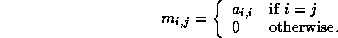
This is known as the (point) Jacobi preconditioner.
It is possible to use this preconditioner without using any extra
storage beyond that of the matrix itself. However, division operations
are usually quite costly, so in practice storage is allocated
for the reciprocals of the matrix diagonal. This strategy applies to
many preconditioners below.
Jack Dongarra
Mon Nov 20 08:52:54 EST 1995
Block Jacobi Methods
Next:
Discussion
Up:
Jacobi Preconditioning
Previous:
Jacobi Preconditioning
Block versions of the Jacobi preconditioner can be derived by a
partitioning of the variables. If the index set  is partitioned as
  with the sets
  mutually
disjoint, then
mutually
disjoint, then

The preconditioner is now a block-diagonal matrix.
Often, natural choices for the partitioning suggest themselves:
- In problems with multiple physical variables per node,
blocks can be formed by grouping the equations per node.
- In structured matrices, such as those from partial differential
equations on regular grids, a partitioning can be based on the
physical domain. Examples are a partitioning along lines in the
2D case, or planes in the 3D case. This will be discussed
further in §
.
- On parallel computers it is natural to let the
partitioning coincide with the division of variables
over the processors.
Jack Dongarra
Mon Nov 20 08:52:54 EST 1995
Discussion
Next:
SSOR preconditioning
Up:
Jacobi Preconditioning
Previous:
Block Jacobi Methods
Jacobi preconditioners need very little storage, even in the block
case, and they are easy to implement. Additionally, on parallel
computers they don't present any particular problems.
On the other hand, more sophisticated preconditioners usually yield
a larger improvement.
Jack Dongarra
Mon Nov 20 08:52:54 EST 1995
SSOR preconditioning
Next:
Incomplete Factorization Preconditioners
Up:
Preconditioners
Previous:
Discussion
The SSOR preconditioner
like the Jacobi preconditioner, can be derived from the coefficient
matrix without any work.
If the original, symmetric, matrix is decomposed as

in its diagonal, lower, and upper triangular part, the SSOR matrix is
defined as

or, parameterized by

The optimal value of the
parameter, like the
parameter in the SOR method, will reduce the number
of iterations to a lower order.
Specifically, for second order elliptic problems a spectral
condition number 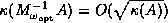 is attainable
(see Axelsson and Barker [.4]AxBa:febook). In practice,
however, the spectral
information needed to calculate the optimal
is prohibitively
expensive to compute.
is attainable
(see Axelsson and Barker [.4]AxBa:febook). In practice,
however, the spectral
information needed to calculate the optimal
is prohibitively
expensive to compute.
The SSOR matrix is given in factored form, so this preconditioner
shares many properties of other factorization-based methods (see
below). For instance, its suitability for vector processors or
parallel architectures
depends strongly on the
ordering of the variables. On the other hand, since this factorization
is given a priori, there is no possibility of breakdown as in
the construction phase of incomplete factorization methods.
Jack Dongarra
Mon Nov 20 08:52:54 EST 1995
Incomplete Factorization Preconditioners
Next:
Creating an incomplete
Up:
Preconditioners
Previous:
SSOR preconditioning
A broad class of preconditioners is based on incomplete factorizations
of the coefficient matrix. We call a factorization incomplete if
during the factorization process certain fill elements,
nonzero elements in the factorization in positions where the original
matrix had a zero, have been
ignored. Such a preconditioner is then given in factored form
with
lower and
upper triangular. The efficacy of the
preconditioner depends on how well
approximates
.
Jack Dongarra
Mon Nov 20 08:52:54 EST 1995
Introduction
Next:
Why Use Templates?
Up:
Templates for the Solution
Previous:
List of Figures
Which of the following statements is true?
- Users want ``black box''Black box: A piece of software that
can be used without knowledge of its inner workings; the user supplies the
input, and the output is more or less guaranteed to be correct.
software that they can use with
complete confidence for general problem classes without having to
understand the fine algorithmic details.
- Users want to be able to tuneTune: Adapt software
for a specific application and computing environment
in order to obtain better performance in that case only.
data structures for a particular
application, even if the software is not as reliable as that
provided for general methods.
It turns out both are true, for different groups of users.
Traditionally, users have asked for and been provided with black box
software in the form of mathematical libraries such as LAPACK
,
LINPACK
, NAG
, and
IMSL
. More recently, the
high-performance community has discovered that they must write custom
software for their problem. Their reasons include inadequate
functionality of existing software libraries, data structures that are
not natural or convenient for a particular problem, and overly general
software that sacrifices too much performance when applied to a
special case of interest.
Can we meet the needs of both groups of users? We believe we can.
Accordingly, in this book, we introduce the use of templates
Template: Description of an
algorithm, abstracting away from implementational details.
A template is a description of a general algorithm rather than the
executable object code or the source code more commonly found in a
conventional software library. Nevertheless, although templates are
general descriptions of key algorithms, they offer whatever degree of
customization the user may desire. For example, they can be
configured for the specific data structure of a problem or for the
specific computing system on which the problem is to run.
We focus on the use of iterative methods for
solving large sparse systems of linear equations.Iterative
method: An algorithm that produces a sequence of approximations to
the solution of a linear system of equations; the length of the
sequence is not given a priori by the size of the system. Usually,
the longer one iterates,
the closer one is able to get to the true solution. See: Direct method.Direct method:
An algorithm that produces the solution to a system of linear equations
in a number of operations that is determined a priori by the size
of the system. In exact arithmetic, a direct method yields the true
solution to the system. See: Iterative method.
Many methods exist for solving such
problems. The trick is to find the most effective method for the
problem at hand. Unfortunately, a method that works well for one
problem type may not work as well for another. Indeed, it may not work
at all.
Thus, besides providing templates, we suggest how to choose and
implement an effective method, and how to specialize a method to
specific matrix types. We restrict ourselves to iterative
methods, which work by repeatedly improving an approximate solution
until it is accurate enough. These methods access the coefficient
matrix
of the linear system only via the
matrix-vector product  (and
perhaps
(and
perhaps  ). Thus the user need only supply a subroutine
for computing
(and perhaps
) given
, which permits full
exploitation of the sparsity or other special structure of
.
). Thus the user need only supply a subroutine
for computing
(and perhaps
) given
, which permits full
exploitation of the sparsity or other special structure of
.
We believe that after reading this book, applications developers will
be able to use templates to get their program running on a parallel
machine quickly. Nonspecialists will know how to choose and implement
an approach to solve a particular problem. Specialists will be able
to assemble and modify their codes-without having to make the huge
investment that has, up to now, been required to tune large-scale
applications for each particular machine. Finally, we hope that all
users will gain a better understanding of the algorithms employed.
While education has not been one of the traditional goals of
mathematical software, we believe that our approach will go a long way
in providing such a valuable service.
Next:
Why Use Templates?
Up:
Templates for the Solution
Previous:
List of Figures
Jack Dongarra
Mon Nov 20 08:52:54 EST 1995
Creating an incomplete factorization
Next:
Solving a system
Up:
Incomplete Factorization Preconditioners
Previous:
Incomplete Factorization Preconditioners
Incomplete factorizations are the first preconditioners we have
encountered so far for which there is a non-trivial creation stage.
Incomplete factorizations may break down (attempted
division by zero pivot) or result in indefinite matrices (negative
pivots) even if the full factorization of the same matrix is
guaranteed to exist and yield a positive definite matrix.
An incomplete factorization is guaranteed to exist for many
factorization strategies if the original matrix is an
-matrix.
This was originally proved by Meijerink and
Van der Vorst
[152]; see
further Beauwens and Quenon
[33],
Manteuffel
[147], and
Van der Vorst
[200].
In cases where pivots are zero or negative, strategies have been
proposed such as substituting an arbitrary positive
number (see Kershaw
[132]), or restarting the factorization
on  for some positive value of
  (see
Manteuffel
[147]).
(see
Manteuffel
[147]).
An important consideration for incomplete
factorization preconditioners is the cost of the factorization process.
Even if the incomplete factorization exists,
the number of operations involved in creating it
is at least as much as for
solving a system with such a coefficient matrix, so the cost may equal
that of one
or more iterations of the iterative method. On parallel computers this
problem is aggravated by the generally poor parallel efficiency of the
factorization.
Such factorization costs can be amortized if the iterative method
takes many iterations, or if the same preconditioner will be used
for several linear systems, for instance in successive time steps or
Newton iterations.
Jack Dongarra
Mon Nov 20 08:52:54 EST 1995
Solving a system with an incomplete factorization
preconditioner
Next:
Point incomplete factorizations
Up:
Creating an incomplete
Previous:
Creating an incomplete
Incomplete factorizations can be given in various forms. If
(with
and
nonsingular triangular matrices),
solving a system proceeds in the usual way
(figure
),

Figure: Preconditioner solve of a system  , with
but often incomplete factorizations are given as  (with
diagonal, and
and
now strictly triangular matrices, determined through
the factorization process).
In that case, one could use either of the following equivalent
formulations for
:
(with
diagonal, and
and
now strictly triangular matrices, determined through
the factorization process).
In that case, one could use either of the following equivalent
formulations for
:

or

In either case, the diagonal elements are used twice (not three times
as the formula for
would lead one to expect), and since only
divisions with
are performed, storing
explicitly is the
practical thing to do.
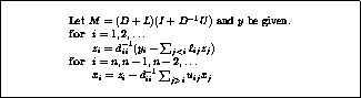
Figure: Preconditioner solve of a system
,
with  .
.
At the cost of some extra storage, one could store  or
, thereby saving some computation.
Solving a system using the first formulation is
outlined in figure
. The second formulation is
slightly harder to implement.
or
, thereby saving some computation.
Solving a system using the first formulation is
outlined in figure
. The second formulation is
slightly harder to implement.
Jack Dongarra
Mon Nov 20 08:52:54 EST 1995
Point incomplete factorizations
Next:
Fill-in strategies
Up:
Incomplete Factorization Preconditioners
Previous:
Solving a system
The most common type of incomplete factorization is based on taking a
set  of matrix positions, and keeping all positions outside this
set equal to zero during the factorization. The resulting
factorization is incomplete in the sense that fill is suppressed.
of matrix positions, and keeping all positions outside this
set equal to zero during the factorization. The resulting
factorization is incomplete in the sense that fill is suppressed.
The set
is usually chosen to encompass all positions
for
which  . A position that is zero in
but not so in an
exact factorization
is called a fill position, and if it is
outside
, the fill there is said to be ``discarded''.
Often,
is chosen to coincide with the set of nonzero positions
in
, discarding all fill. This factorization type is called
the
factorization: the Incomplete
factorization of
level zero
.
. A position that is zero in
but not so in an
exact factorization
is called a fill position, and if it is
outside
, the fill there is said to be ``discarded''.
Often,
is chosen to coincide with the set of nonzero positions
in
, discarding all fill. This factorization type is called
the
factorization: the Incomplete
factorization of
level zero
.
We can describe an incomplete factorization formally as

Meijerink and Van der Vorst
[152] proved that, if
is
an
-matrix, such a factorization exists for any choice of
, and
gives a symmetric positive definite matrix if
is symmetric
positive definite. Guidelines for allowing levels of fill were given
by Meijerink and Van der Vorst in
[153].
Jack Dongarra
Mon Nov 20 08:52:54 EST 1995
Fill-in strategies
Next:
Simple cases: and
Up:
Point incomplete factorizations
Previous:
Point incomplete factorizations
There are two major strategies for accepting or discarding fill-in,
one structural, and one numerical. The structural strategy is that of
accepting fill-in only to a certain level. As was already pointed out above,
any zero location
in
filling in (say in step
)
is assigned a fill level value

If  was already nonzero, the level value is not changed.
The numerical fill strategy is that of `drop tolerances':
fill is ignored if it is too small, for a suitable definition of
`small'. Although this definition makes more sense mathematically, it
is harder to implement in practice, since the amount of storage needed
for the factorization is not easy to predict.
See
[157]
[20] for discussions of
preconditioners using drop tolerances.
Jack Dongarra
Mon Nov 20 08:52:54 EST 1995
Simple cases: <IMG ALIGN=BOTTOM SRC="http://www.netlib.org/utk/papers/templates/_22900_tex2html_wrap6165.gif">
and <IMG ALIGN=BOTTOM SRC="http://www.netlib.org/utk/papers/templates/_22900_tex2html_wrap6389.gif">
-<IMG ALIGN=BOTTOM SRC="http://www.netlib.org/utk/papers/templates/_22900_tex2html_wrap7381.gif">
Next:
Special cases: central
Up:
Point incomplete factorizations
Previous:
Fill-in strategies
For the
method, the incomplete factorization produces no
nonzero elements beyond the sparsity structure
of the original matrix, so that the preconditioner at worst
takes exactly as much space to store as the original matrix. In a
simplified version of
, called
-
(Pommerell
[174]), even less is needed. If not only we
prohibit fill-in elements, but we also alter only the diagonal
elements (that is, any alterations of off-diagonal elements are
ignored
),
we have the following situation.
Splitting the coefficient matrix into its diagonal, lower
triangular, and upper triangular parts as
, the
preconditioner can be written as  where
is the
diagonal matrix containing the pivots generated. Generating this
preconditioner is described in figure
.
where
is the
diagonal matrix containing the pivots generated. Generating this
preconditioner is described in figure
.
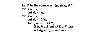
Figure: Construction of a
-
incomplete
factorization preconditioner, storing the inverses
of the pivots
Since we use the
upper and lower triangle of the matrix unchanged, only storage space
for
is needed. In fact, in order to avoid division operations
during the preconditioner solve stage we store
rather than
.
Remark: the resulting lower and upper factors of the preconditioner have
only nonzero elements in the set
, but this fact is in general not
true for the preconditioner
itself.
The fact that the
-
preconditioner contains the off-diagonal
parts of the original matrix was used by
Eisenstat
[91] to derive at a more
efficient implementation of preconditioned CG. This new
implementation merges the application of the tridiagonal factors of
the matrix and the preconditioner, thereby saving a substantial number
of operations per iteration.
Jack Dongarra
Mon Nov 20 08:52:54 EST 1995
Special cases: central differences
Next:
Modified incomplete factorizations
Up:
Point incomplete factorizations
Previous:
Simple cases: and
We will now consider the special case of
a matrix derived from central differences on a Cartesian product grid.
In this case the
and
-
factorizations coincide, and,
as remarked above, we only have to calculate the pivots of the
factorization; other elements in the triangular factors are equal to
off-diagonal elements of
.
In the following we will assume a natural, line-by-line, ordering of
the grid points.
Letting
,
be coordinates in a regular 2D grid, it is easy to see
that the pivot on grid point
is only determined by
pivots on points  and
and  . If there are
points on
each of
grid lines,
we get the following generating relations for the pivots:
. If there are
points on
each of
grid lines,
we get the following generating relations for the pivots:
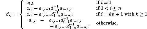
Conversely, we can describe the factorization algorithmically as

In the above we have assumed that the variables in the problem
are ordered according to the so-called ``natural ordering'': a
sequential numbering of the grid lines and the points within each grid
line. Below we will encounter different orderings of the variables.
Jack Dongarra
Mon Nov 20 08:52:54 EST 1995
Modified incomplete factorizations
Next:
Vectorization of the
Up:
Point incomplete factorizations
Previous:
Special cases: central
One modification to the basic idea of incomplete factorizations is as
follows:
If the product  is nonzero, and fill is not allowed in position
,
instead of simply discarding this fill quantity subtract it from
the diagonal element
.
Such a factorization scheme is usually called a ``modified incomplete
factorization''.
is nonzero, and fill is not allowed in position
,
instead of simply discarding this fill quantity subtract it from
the diagonal element
.
Such a factorization scheme is usually called a ``modified incomplete
factorization''.
Mathematically this corresponds to forcing the preconditioner to have
the same rowsums as the original matrix.
One reason for considering modified incomplete factorizations is the
behavior of the spectral condition number of the preconditioned
system. It was mentioned above that for second order elliptic
equations the condition number of the
coefficient matrix is  as a function of the discretization
mesh width. This order of magnitude is preserved by simple incomplete
factorizations, although usually a reduction by a large constant
factor is obtained.
as a function of the discretization
mesh width. This order of magnitude is preserved by simple incomplete
factorizations, although usually a reduction by a large constant
factor is obtained.
Modified factorizations are of interest because, in
combination with small perturbations, the spectral condition number of
the preconditioned system can be of a lower order.
It was first proved by Dupont, Kendall and
Rachford
[81] that
a modified incomplete factorization of  gives
gives
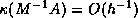 for the central difference case. More
general proofs are given by Gustafsson
[112],
Axelsson and Barker [.2]AxBa:febook, and
Beauwens
[32]
[31].
for the central difference case. More
general proofs are given by Gustafsson
[112],
Axelsson and Barker [.2]AxBa:febook, and
Beauwens
[32]
[31].
Instead of keeping row sums constant, one can also keep column
sums constant.
In computational fluid mechanics this idea is justified with the argument
that the material balance stays constant over all iterates.
(Equivalently, one wishes to avoid `artificial
diffusion'.)
Appleyard and Cheshire
[4] observed that if
and
have the same column sums, the choice

guarantees
that the sum of the elements in  (the material balance error) is
zero, and that all further
(the material balance error) is
zero, and that all further  have elements summing to zero.
Modified incomplete factorizations can break down,
especially when the variables are numbered other than in the natural
row-by-row ordering. This was noted by Chan and
Kuo
[50], and a full analysis was given by
Eijkhout
[86] and Notay
[161].
A slight variant of modified incomplete factorizations consists of the
class of ``relaxed incomplete factorizations''. Here the fill is
multiplied by a parameter  before it is subtracted from
the diagonal; see
Ashcraft and Grimes
[11],
Axelsson and Lindskog
[19]
[18],
Chan
[44],
Eijkhout
[86],
Notay
[162],
Stone
[194], and
Van der Vorst
[204].
For the dangers of MILU in the presence of rounding error, see
Van der Vorst
[206].
before it is subtracted from
the diagonal; see
Ashcraft and Grimes
[11],
Axelsson and Lindskog
[19]
[18],
Chan
[44],
Eijkhout
[86],
Notay
[162],
Stone
[194], and
Van der Vorst
[204].
For the dangers of MILU in the presence of rounding error, see
Van der Vorst
[206].
Next:
Vectorization of the
Up:
Point incomplete factorizations
Previous:
Special cases: central
Jack Dongarra
Mon Nov 20 08:52:54 EST 1995
Vectorization of the preconditioner solve
Next:
Parallelizing the preconditioner
Up:
Point incomplete factorizations
Previous:
Modified incomplete factorizations
At first it may appear that the sequential time of solving a
factorization is of the order of the number of variables, but things
are not quite that bad. Consider the special case of central
differences on a regular domain of
points. The variables
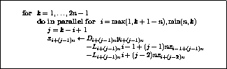
Figure: Wavefront solution of  from a central difference problem
on a domain of
from a central difference problem
on a domain of  points.
on any diagonal in the domain, that is,
in locations
with  , depend
only on those on the previous diagonal, that is, with
, depend
only on those on the previous diagonal, that is, with  .
Therefore it is possible to process the operations on such a diagonal,
or `wavefront'
,
in parallel (see figure
),
or have a vector computer pipeline them;
see Van der Vorst
[205]
[203].
.
Therefore it is possible to process the operations on such a diagonal,
or `wavefront'
,
in parallel (see figure
),
or have a vector computer pipeline them;
see Van der Vorst
[205]
[203].
Another way of vectorizing the solution of the triangular factors is
to use some form of expansion of the inverses of the factors.
Consider for a moment a lower triangular matrix, normalized to
the form  where
is strictly lower triangular). Its
inverse can be given as either of the following two series:
where
is strictly lower triangular). Its
inverse can be given as either of the following two series:

(The first series is called a ``Neumann expansion'', the second an
``Euler expansion''. Both series are finite, but their length
prohibits practical use of this fact.)
Parallel or vectorizable preconditioners can be derived from an
incomplete factorization by taking a small number of terms in either
series.
Experiments indicate that a small number of terms, while
giving high execution rates, yields almost the full precision of the
more recursive triangular solution (see
Axelsson and Eijkhout
[15] and
Van der Vorst
[201]).
There are some practical considerations in implementing these
expansion algorithms. For instance, because of the normalization the
in equation (
) is not  . Rather, if we
have a preconditioner (as described in section
)
described by
. Rather, if we
have a preconditioner (as described in section
)
described by

then we write

Now we can choose whether or not to store the product  .
Doing so doubles the storage requirements for the matrix, not doing so
means that separate multiplications by
and
have to be
performed in the expansion.
.
Doing so doubles the storage requirements for the matrix, not doing so
means that separate multiplications by
and
have to be
performed in the expansion.
Figure: Preconditioning step algorithm for
a Neumann expansion  of an incomplete factorization
  .
.
Suppose then that the products  and
and  have been
stored. We then define
by
have been
stored. We then define
by

and replace solving a system
for
by computing  .
This algorithm is given in figure
.
.
This algorithm is given in figure
.
Next:
Parallelizing the preconditioner
Up:
Point incomplete factorizations
Previous:
Modified incomplete factorizations
Jack Dongarra
Mon Nov 20 08:52:54 EST 1995
Parallelizing the preconditioner solve
Next:
Block factorization methods
Up:
Point incomplete factorizations
Previous:
Vectorization of the
The algorithms for vectorization outlined above can be used on
parallel computers. For instance, variables on a wavefront
can be
processed in parallel, by dividing the wavefront over processors.
More radical approaches for increasing the parallelism in incomplete
factorizations are based on a renumbering of the problem variables.
For instance, on rectangular domains one could start numbering the
variables from all four corners simultaneously, thereby creating
four simultaneous wavefronts, and therefore four-fold parallelism
(see Dongarra, et al.
[71],
Van der Vorst
[204]
[202])
.
The most extreme case is the red/black ordering
(or for more general matrices the multi-color ordering) which gives
the absolute minimum number of sequential steps.
Multi-coloring is also an attractive method for vector computers.
Since points of one color are uncoupled, they can be processed as one
vector; see Doi
[68],
Melhem
[154], and Poole and
Ortega
[176].
However, for such ordering strategies there is usually a trade-off
between the degree of parallelism and the resulting number of
iterations. The reason for this is that a different ordering may give
rise to a different error matrix, in particular the norm of the error
matrix may vary considerably between orderings.
See experimental results by Duff and Meurant
[79] and a
partial explanation of them by Eijkhout
[85].
Jack Dongarra
Mon Nov 20 08:52:54 EST 1995
Block factorization methods
Next:
The idea behind
Up:
Incomplete Factorization Preconditioners
Previous:
Parallelizing the preconditioner
We can also consider block variants of preconditioners for accelerated
methods. Block methods are normally feasible if the problem domain is
a Cartesian product grid; in that case a natural division in lines (or
planes in the 3-dimensional case), can be used for blocking, though
incomplete factorizations are not as effective in the 3-dimensional
case; see for instance Kettler
[134].
In such a blocking scheme for Cartesian product grids,
both the size and number of the
blocks increases with the overall problem size.
Jack Dongarra
Mon Nov 20 08:52:54 EST 1995
Why Use Templates?
Next:
What Methods Are
Up:
Introduction
Previous:
Introduction
Templates offer three significant advantages. First, templates are
general and reusable. Thus, they can simplify ports to diverse
machines. This feature is important given the diversity
of parallel architectures.
Second, templates exploit the expertise of two distinct groups. The
expert numerical analyst creates a template reflecting in-depth
knowledge of a specific numerical technique. The computational scientist
then provides ``value-added'' capability to the general template
description, customizing it for specific contexts or applications
needs.
And third, templates are not language specific. Rather, they are
displayed in an Algol-like structure, which is readily translatable
into the target language such as FORTRAN (with the use of the
Basic Linear Algebra Subprograms, or BLAS
,
whenever possible) and C. By using these familiar styles, we
believe that the users will have trust in the algorithms. We also
hope that users will gain a better understanding of numerical
techniques and parallel programming.
For each template, we provide some or all of the following:
- a mathematical description of the flow of the iteration;
- discussion of convergence and stopping criteria;
- suggestions for applying a method to special matrix types
(e.g., banded systems);
- advice for tuning (for example, which preconditioners are
applicable and which are not);
- tips on parallel implementations; and
- hints as to when to use a method, and why.
For each of the templates, the following can be obtained via electronic mail.
- a MATLAB
implementation based on
dense matrices;
- a FORTRAN-77
program with calls to
BLAS
;
- a C++
template implementation for matrix/vector classes.
See Appendix
for details.
Jack Dongarra
Mon Nov 20 08:52:54 EST 1995
The idea behind block factorizations
Next:
Approximate inverses
Up:
Block factorization methods
Previous:
Block factorization methods
The starting point for an incomplete block factorization is a
partitioning of the matrix, as mentioned in §
.
Then an incomplete factorization is performed using the matrix blocks
as basic entities (see Axelsson
[12] and Concus, Golub
and Meurant
[57] as
basic references).
The most important difference with point methods arises in the
inversion of the pivot blocks. Whereas inverting a scalar is easily
done, in the block case two problems arise. First, inverting
the pivot block is likely to be a costly operation. Second, initially the
diagonal blocks of the matrix are likely to be be sparse
and we would like to maintain this type of
structure throughout the factorization.
Hence the need for approximations of inverses arises.
Figure: Block version of a
-
factorization
In addition to this, often fill-in in off-diagonal blocks is discarded
altogether. Figure
describes an incomplete block
factorization that is analogous to the
-
factorization
(section
) in that it only updates the diagonal blocks.
As in the case of incomplete point factorizations, the existence of
incomplete block methods is guaranteed if the coefficient
matrix is an
-matrix. For a general proof, see
Axelsson
[13].
Jack Dongarra
Mon Nov 20 08:52:54 EST 1995
Approximate inverses
Next:
The special case
Up:
Block factorization methods
Previous:
The idea behind
In block factorizations a pivot block is generally forced to be
sparse, typically of banded form, and that we need an approximation to
its inverse that has a similar structure. Furthermore, this
approximation should be easily computable, so we rule out the option
of calculating the full inverse and taking a banded part of it.
The simplest approximation to
is the diagonal matrix
of
the reciprocals of the diagonal of
:  .
.

Figure: Algorithm for approximating the inverse of a banded matrix
Other possibilities were considered by
Axelsson and Eijkhout
[15],
Axelsson and Polman
[21],
Concus, Golub and Meurant
[57],
Eijkhout and Vassilevski
[90],
Kolotilina and Yeremin
[141],
and Meurant
[155]. One particular
example is given in figure
. It has the attractive
theoretical property that, if the original matrix is symmetric
positive definite and a factorization with positive diagonal
can
be made, the approximation to the inverse is again symmetric positive
definite.
Banded approximations to the inverse of banded matrices have a
theoretical justification. In the context of partial differential
equations the diagonal blocks of the coefficient matrix are usually
strongly diagonally dominant. For such matrices, the elements of the
inverse have a size that is exponentially decreasing in their distance
from the main diagonal. See Demko, Moss and
Smith
[65] for a general
proof, and Eijkhout and Polman
[89] for a more detailed
analysis in the
-matrix case.
Jack Dongarra
Mon Nov 20 08:52:54 EST 1995
The special case of block tridiagonality
Next:
Two types of
Up:
Block factorization methods
Previous:
Approximate inverses
In many applications, a block tridiagonal structure can be found in
the coefficient matrix. Examples are problems on a 2D regular grid if
the blocks correspond to lines of grid points, and problems on a
regular 3D grid, if the blocks correspond to planes of grid points.
Even if such a block tridiagonal structure does not arise naturally,
it can be imposed by renumbering the variables in a Cuthill-McKee
ordering
[60].

Figure: Incomplete block factorization of a block tridiagonal matrix
Such a matrix has incomplete block factorizations of a particularly
simple nature: since no fill can occur outside the diagonal
blocks  ,
all properties follow from our treatment of the pivot blocks. The
generating recurrence for the pivot blocks also takes a simple form,
see figure
. After the factorization we are left
with sequences of
,
all properties follow from our treatment of the pivot blocks. The
generating recurrence for the pivot blocks also takes a simple form,
see figure
. After the factorization we are left
with sequences of  block forming the pivots, and of
  blocks
approximating their inverses.
blocks
approximating their inverses.
Jack Dongarra
Mon Nov 20 08:52:54 EST 1995
Two types of incomplete block factorizations
Next:
Blocking over systems
Up:
Block factorization methods
Previous:
The special case
One reason that block methods are of interest is that they are
potentially more suitable for vector computers and parallel
architectures. Consider the block factorization

where
is the block diagonal matrix of pivot blocks,
and
,
are the block lower and upper triangle of the factorization;
they coincide with
,  in the case of a block tridiagonal
matrix.
in the case of a block tridiagonal
matrix.
We can turn this into an incomplete factorization by replacing the
block diagonal matrix of pivots
by the block diagonal matrix of
incomplete factorization pivots  , giving

For factorizations of this type (which covers all
methods in Concus, Golub and Meurant
[57] and
Kolotilina and Yeremin
[141]) solving
a linear system means solving
smaller systems with the
matrices.
Alternatively, we can replace
by a
the inverse of the block diagonal matrix of the
approximations to the inverses of the pivots,  , giving

For this second type (which
was discussed by Meurant
[155], Axelsson and
Polman
[21] and Axelsson and
Eijkhout
[15]) solving
a system with
entails multiplying by the
blocks.
Therefore, the second type has a much higher potential for
vectorizability. Unfortunately, such a factorization is theoretically
more troublesome; see the above references or Eijkhout and
Vassilevski
[90].
Jack Dongarra
Mon Nov 20 08:52:54 EST 1995
Blocking over systems of partial differential
equations
Next:
Incomplete LQ factorizations
Up:
Incomplete Factorization Preconditioners
Previous:
Two types of
If the physical problem has several variables per grid point, that is,
if there are several coupled partial differential equations, it is
possible to introduce blocking in a natural way.
Blocking of the equations (which gives a small number of very large
blocks) was used by Axelsson and Gustafsson
[17] for
the equations of linear
elasticity, and blocking of the
variables per node (which gives many very small blocks) was used
by Aarden and Karlsson
[1] for the
semiconductor
equations. A systematic comparison of the two approaches was made
by Bank, et al.
[26].
Jack Dongarra
Mon Nov 20 08:52:54 EST 1995
Incomplete LQ factorizations
Next:
Polynomial preconditioners
Up:
Incomplete Factorization Preconditioners
Previous:
Blocking over systems
Saad
[184] proposes to construct an incomplete LQ factorization
of a general sparse matrix. The idea is to orthogonalize the rows
of the matrix by a Gram-Schmidt process (note that in sparse matrices,
most rows are typically orthogonal already, so that standard Gram-Schmidt
may be not so bad as in general). Saad suggest dropping strategies for
the fill-in produced in the orthogonalization process. It turns out that
the resulting incomplete L factor can be viewed as the incomplete Cholesky
factor of the matrix
. Experiments show that using
in a CG
process for the normal equations:  is effective for
some relevant problems.
is effective for
some relevant problems.
Jack Dongarra
Mon Nov 20 08:52:54 EST 1995
Polynomial preconditioners
Next:
Preconditioners from properties
Up:
Preconditioners
Previous:
Incomplete LQ factorizations
So far, we have described preconditioners in only one of two classes:
those that approximate the coefficient
matrix, and where linear systems with the preconditioner as
coefficient matrix are easier to solve than the original system.
Polynomial preconditioners can be considered as members of the
second class of preconditioners:
direct approximations of the inverse of the coefficient matrix.
Suppose that the coefficient matrix
of the linear system is
normalized to
the form  , and that the spectral radius of
is less than
one. Using the Neumann series, we can write the inverse of
as
, and that the spectral radius of
is less than
one. Using the Neumann series, we can write the inverse of
as
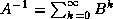 ,
so an approximation may be derived by truncating this infinite series.
Since the iterative methods we are considering are already based on
the idea of applying polynomials in the coefficient matrix to the
initial residual, there are analytic connections between the basic
method and polynomially accelerated one.
,
so an approximation may be derived by truncating this infinite series.
Since the iterative methods we are considering are already based on
the idea of applying polynomials in the coefficient matrix to the
initial residual, there are analytic connections between the basic
method and polynomially accelerated one.
Dubois, Greenbaum and Rodrigue
[77]
investigated the relationship between a basic method
using a splitting  , and a polynomially preconditioned method
with
, and a polynomially preconditioned method
with
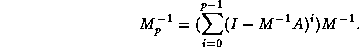
The basic result is that for classical methods,
steps of the polynomially preconditioned method are
exactly equivalent to
 steps of the original method; for accelerated
methods, specifically the Chebyshev method, the preconditioned
iteration can improve the number of iterations by at most a factor
of
.
steps of the original method; for accelerated
methods, specifically the Chebyshev method, the preconditioned
iteration can improve the number of iterations by at most a factor
of
.
Although there is no gain in the number of times the coefficient
matrix is applied, polynomial preconditioning does eliminate a large
fraction of the inner
products and update operations, so there may be an overall increase in
efficiency.
Let us define a polynomial preconditioner more abstractly as any
polynomial  normalized to
  . Now the choice of the
best polynomial preconditioner becomes that of choosing the best
polynomial that minimizes
. Now the choice of the
best polynomial preconditioner becomes that of choosing the best
polynomial that minimizes  . For the choice of the
infinity norm we thus obtain Chebyshev polynomials, and they require
estimates of both a lower and upper bound on the spectrum of
.
These estimates may be derived from the conjugate gradient iteration
itself; see §
.
. For the choice of the
infinity norm we thus obtain Chebyshev polynomials, and they require
estimates of both a lower and upper bound on the spectrum of
.
These estimates may be derived from the conjugate gradient iteration
itself; see §
.
Since an accurate lower bound on the spectrum of
may be hard to
obtain, Johnson, Micchelli and Paul
[126]
and Saad
[183] propose least
squares polynomials based on several weight functions.
These functions only require an upper bound and this is easily
computed, using for instance the ``Gerschgorin bound''
 ; see [.4]Va:book.
Experiments comparing Chebyshev and least squares polynomials can be
found in Ashby, Manteuffel and Otto
[8].
; see [.4]Va:book.
Experiments comparing Chebyshev and least squares polynomials can be
found in Ashby, Manteuffel and Otto
[8].
Application of polynomial preconditioning to symmetric indefinite
problems is described by Ashby, Manteuffel and
Saylor
[9]. There the
polynomial is chosen so that it transforms the system into a
definite one.
Next:
Preconditioners from properties
Up:
Preconditioners
Previous:
Incomplete LQ factorizations
Jack Dongarra
Mon Nov 20 08:52:54 EST 1995
Preconditioners from properties of the
differential equation
Next:
Preconditioning by the
Up:
Preconditioners
Previous:
Polynomial preconditioners
A number of preconditioners exist that derive their justification from
properties of the underlying partial differential equation. We will
cover some of them here (see also §
and §
). These preconditioners usually involve more
work than the types discussed above, however, they allow for
specialized faster solution methods.
Jack Dongarra
Mon Nov 20 08:52:54 EST 1995
Preconditioning by the symmetric part
Next:
The use of
Up:
Preconditioners from properties
Previous:
Preconditioners from properties
In §
we pointed out that conjugate
gradient methods for non-selfadjoint systems require the storage of
previously calculated vectors. Therefore it is somewhat remarkable
that preconditioning by the symmetric part  of the coefficient matrix
leads to a method that does not need this extended storage.
Such a method was proposed by Concus and Golub
[56]
and Widlund
[216].
of the coefficient matrix
leads to a method that does not need this extended storage.
Such a method was proposed by Concus and Golub
[56]
and Widlund
[216].
However, solving a system with the symmetric part of a matrix may be
no easier than solving a system with the full matrix. This problem may
be tackled by imposing a nested iterative method, where a
preconditioner based on the symmetric part is used.
Vassilevski
[212] proved that the efficiency of this
preconditioner for the symmetric part carries over to the outer
method.
Jack Dongarra
Mon Nov 20 08:52:54 EST 1995
The use of fast solvers
Next:
Alternating Direction Implicit
Up:
Preconditioners from properties
Previous:
Preconditioning by the
In many applications, the coefficient matrix is symmetric and positive
definite. The reason for this is usually that the partial differential
operator from which it is derived is self-adjoint, coercive, and bounded
(see Axelsson and Barker [.2]AxBa:febook).
It follows that for the coefficient
matrix
the following relation holds for any matrix
from a
similar differential equation:
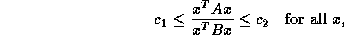
where  ,
,  do not depend on the matrix size. The importance of
this is that the use of
as a preconditioner gives an iterative
method with a number of iterations that does not depend on the matrix size.
do not depend on the matrix size. The importance of
this is that the use of
as a preconditioner gives an iterative
method with a number of iterations that does not depend on the matrix size.
Thus we can precondition our original matrix by one derived from a
different PDE, if one can be found that has attractive properties as
preconditioner.
The most common choice is to take a matrix from a separable PDE. A system involving such a matrix can be solved with
various so-called ``fast solvers'', such as FFT methods, cyclic
reduction, or the generalized marching algorithm
(see Dorr
[75],
Swarztrauber
[195], Bank
[25] and
Bank and Rose
[27]).
As a simplest example, any elliptic operator can be preconditioned
with the Poisson operator, giving the iterative method

In Concus and Golub
[59] a transformation of this
method is considered to speed up the convergence.
As another example, if the original matrix arises from

the preconditioner can be formed from

An extension to the non-self adjoint case is considered
by Elman and Schultz
[94].
Fast solvers are attractive in that the number of operations they
require is (slightly higher than) of the order of the number of
variables. Coupled with the fact that the number of iterations in the
resulting preconditioned iterative methods is independent of the
matrix size, such methods are close to optimal. However, fast solvers
are usually only applicable if the physical domain is a rectangle or
other Cartesian product structure. (For a domain consisting of a
number of such pieces, domain decomposition methods can be used;
see §
).
Next:
Alternating Direction Implicit
Up:
Preconditioners from properties
Previous:
Preconditioning by the
Jack Dongarra
Mon Nov 20 08:52:54 EST 1995
What Methods Are Covered?
Next:
Iterative Methods
Up:
Introduction
Previous:
Why Use Templates?
Many iterative methods have been developed and it is impossible to
cover them all. We chose the methods below either because they
illustrate the historical development of iterative methods, or because
they represent the current state-of-the-art for solving large sparse
linear systems. The methods we discuss are:
- Jacobi
- Gauss-Seidel
- Successive Over-Relaxation (SOR
)
- Symmetric Successive Over-Relaxation (SSOR
)
- Conjugate Gradient (CG
)
- Minimal Residual (MINRES
)
and Symmetric LQ (SYMMLQ
)
- Conjugate Gradients on the Normal Equations
(CGNE
and CGNR
)
- Generalized Minimal Residual (GMRES
)
- Biconjugate Gradient (BiCG
)
- Quasi-Minimal Residual (QMR
)
- Conjugate Gradient Squared (CGS
)
- Biconjugate Gradient Stabilized (Bi-CGSTAB
)
- Chebyshev
Iteration
For each method we present a general description, including a
discussion of the history of the method and numerous references to the
literature. We also give the mathematical conditions for selecting a
given method.
We do not intend to write a ``cookbook'', and have deliberately
avoided the words ``numerical recipes'', because these phrases imply
that our algorithms can be used blindly without knowledge of the
system of equations. The state of the art in iterative methods does
not permit this: some knowledge about the linear system is needed to
guarantee convergence of these algorithms, and generally the more that
is known the more the algorithm can be tuned. Thus, we have chosen to
present an algorithmic outline, with guidelines for choosing a method
and implementing it on particular kinds of high-performance machines.
We also discuss the use of preconditioners and relevant data storage
issues.
Jack Dongarra
Mon Nov 20 08:52:54 EST 1995
Alternating Direction Implicit methods
Next:
Related Issues
Up:
Preconditioners from properties
Previous:
The use of
The Poisson differential operator can be split in a natural way
as the sum of two operators:

Now let  ,
,  be discretized representations of
  ,
,  . Based on the observation that
 , iterative schemes
such as
, iterative schemes
such as

with suitable choices of  and
and  have been proposed.
This alternating direction implicit, or ADI, method was first
proposed as a solution method for parabolic equations. The  are then approximations on subsequent time steps. However, it can also
be used for the steady state, that is, for solving elliptic equations.
In that case, the
become subsequent iterates;
see D'Yakonov
[82],
Fairweather, Gourlay and Mitchell
[97],
Hadjidimos
[119], and
Peaceman and Rachford
[173].
Generalization
of this scheme to variable coefficients or fourth order elliptic
problems is relatively straightforward.
are then approximations on subsequent time steps. However, it can also
be used for the steady state, that is, for solving elliptic equations.
In that case, the
become subsequent iterates;
see D'Yakonov
[82],
Fairweather, Gourlay and Mitchell
[97],
Hadjidimos
[119], and
Peaceman and Rachford
[173].
Generalization
of this scheme to variable coefficients or fourth order elliptic
problems is relatively straightforward.
The above method is implicit since it requires systems solutions, and it
alternates the
and
(and if necessary
) directions. It is
attractive from a practical point of view (although mostly on tensor
product grids), since solving a system with, for instance,
a matrix  entails only a number of uncoupled tridiagonal
solutions. These need very little storage over that needed for the
matrix, and they can be executed in parallel
, or one can vectorize
over them.
entails only a number of uncoupled tridiagonal
solutions. These need very little storage over that needed for the
matrix, and they can be executed in parallel
, or one can vectorize
over them.
A theoretical reason that ADI preconditioners are of interest is that
they can be shown to be
spectrally equivalent to the original coefficient matrix. Hence the
number of iterations is bounded independent of the condition number.
However, there is a problem of data distribution. For vector
computers, either the system solution with
or with
will
involve very large strides: if columns of variables in the grid are
stored contiguously, only the solution with
will involve
contiguous data. For the
the stride equals the number of
variables in a column.
On parallel machines an efficient solution is possible if the
processors are arranged in a  grid. During, e.g., the
solve, every processor row then works independently of other
rows. Inside each row, the processors can work together, for instance
using a Schur complement method. With sufficient network bandwidth
this will essentially reduce the time
to that for solving any of the subdomain
systems plus the time for the interface system. Thus, this method will
be close to optimal.
grid. During, e.g., the
solve, every processor row then works independently of other
rows. Inside each row, the processors can work together, for instance
using a Schur complement method. With sufficient network bandwidth
this will essentially reduce the time
to that for solving any of the subdomain
systems plus the time for the interface system. Thus, this method will
be close to optimal.
Next:
Related Issues
Up:
Preconditioners from properties
Previous:
The use of
Jack Dongarra
Mon Nov 20 08:52:54 EST 1995
Related Issues
Next:
Complex Systems
Up:
Templates for the Solution
Previous:
Alternating Direction Implicit
Jack Dongarra
Mon Nov 20 08:52:54 EST 1995
Complex Systems
Next:
Stopping Criteria
Up:
Related Issues
Previous:
Related Issues
Conjugate gradient methods for real symmetric systems can be applied
to complex Hermitian systems in a straightforward manner. For
non-Hermitian complex systems we distinguish two cases. In general,
for any coefficient matrix a CGNE method is possible,
that is, a conjugate gradients method on the normal equations
 ,
or one can split the system into real and complex parts and use
a method such as GMRES on the resulting real nonsymmetric system.
However, in certain practical situations the complex system is
non-Hermitian but symmetric.
,
or one can split the system into real and complex parts and use
a method such as GMRES on the resulting real nonsymmetric system.
However, in certain practical situations the complex system is
non-Hermitian but symmetric.
Complex symmetric systems can be solved by a classical conjugate
gradient or Lanczos method, that is, with short recurrences, if the
complex inner product  is replaced by
  .
Like the BiConjugate Gradient method, this method is susceptible to
breakdown, that is, it can happen that
.
Like the BiConjugate Gradient method, this method is susceptible to
breakdown, that is, it can happen that  for
for  .
A look-ahead strategy can remedy this in most
cases (see Freund
[100]
and Van der Vorst and Melissen
[208]).
.
A look-ahead strategy can remedy this in most
cases (see Freund
[100]
and Van der Vorst and Melissen
[208]).
Jack Dongarra
Mon Nov 20 08:52:54 EST 1995
Stopping Criteria
Next:
More Details about
Up:
Related Issues
Previous:
Complex Systems
Stopping criterion: Since an iterative method computes successive
approximations to the solution of a linear system, a practical test is needed
to determine when to stop the iteration. Ideally this test would measure
the distance of the last iterate to the true solution, but this is not
possible. Instead, various other metrics are used, typically involving
the residual.
Forward error: The difference between a computed iterate and
the true solution of a linear system, measured in some vector norm.
Backward error: The size of perturbations
of
the coefficient matrix and
of the right hand side
of a linear system, such that the computed iterate
is the
solution of
.
An iterative method produces a sequence  of vectors
converging to the vector
satisfying the
system
.
To be effective, a method must decide when to stop. A good stopping
criterion should
of vectors
converging to the vector
satisfying the
system
.
To be effective, a method must decide when to stop. A good stopping
criterion should
- identify when the error
 is small
enough to stop,
is small
enough to stop,
- stop if the error is no longer decreasing or decreasing too slowly, and
- limit the maximum amount of time spent iterating.
For the user wishing to read as little as possible,
the following simple stopping criterion will likely be adequate.
The user must supply the quantities
 ,
,  , stop_tol, and preferably also
  :
:
- The integer
is the maximum number of iterations the algorithm
will be permitted to perform.
- The real number
is a norm of
. Any reasonable
(order of magnitude) approximation of the absolute value of
the largest entry of the matrix
will do.
- The real number
is a norm of
. Again, any
reasonable approximation of the
absolute value of the largest entry of
will do.
- The real number stop_tol measures how small the user wants
the residual
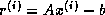 of the ultimate solution
to be. One way to choose stop_tol is as the
approximate uncertainty in the entries of
and
relative to
and
, respectively. For example, choosing stop_tol
of the ultimate solution
to be. One way to choose stop_tol is as the
approximate uncertainty in the entries of
and
relative to
and
, respectively. For example, choosing stop_tol
 means that the user considers the entries of
and
to have errors in the range
means that the user considers the entries of
and
to have errors in the range  and
and  , respectively. The algorithm will compute
no more
accurately than its inherent uncertainty warrants. The user should
choose stop_tol less than one and greater than the machine
precision
, respectively. The algorithm will compute
no more
accurately than its inherent uncertainty warrants. The user should
choose stop_tol less than one and greater than the machine
precision  .
.
Here is the algorithm:
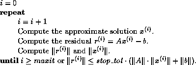
Note that if
does not change much from step to step, which occurs
near convergence, then  need not be recomputed.
If
is not available, the stopping criterion may be replaced with
the generally stricter criterion
need not be recomputed.
If
is not available, the stopping criterion may be replaced with
the generally stricter criterion

In either case, the final error bound is
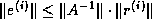 .
If an estimate of
.
If an estimate of  is available, one may also use the stopping
criterion
is available, one may also use the stopping
criterion

which guarantees that the relative error  in the computed solution is bounded by stop_tol.
Next:
More Details about
Up:
Related Issues
Previous:
Complex Systems
Jack Dongarra
Mon Nov 20 08:52:54 EST 1995
More Details about Stopping Criteria
Next:
When or is
Up:
Stopping Criteria
Previous:
Stopping Criteria
Ideally we would like to stop when the magnitudes of entries of the error
 fall below a user-supplied threshold.
But
fall below a user-supplied threshold.
But  is hard to estimate directly, so
we use the residual
instead, which is
more readily computed. The rest of this section describes how to measure
the sizes of vectors
and
, and how to bound
in terms of
.
is hard to estimate directly, so
we use the residual
instead, which is
more readily computed. The rest of this section describes how to measure
the sizes of vectors
and
, and how to bound
in terms of
.
We will measure errors using vector and matrix norms.
The most common vector norms are:
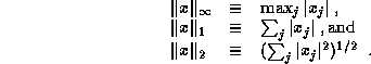
For some algorithms we may also use the norm
 , where
is a fixed nonsingular
matrix and
, where
is a fixed nonsingular
matrix and  is one of
  ,
, or
.
Corresponding to these vector norms are three matrix norms:
,
, or
.
Corresponding to these vector norms are three matrix norms:
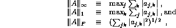
as well as 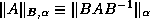 .
We may also use the matrix norm
.
We may also use the matrix norm
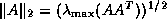 , where
denotes the largest eigenvalue.
Henceforth
, where
denotes the largest eigenvalue.
Henceforth  and
will refer to any mutually
consistent pair of the above.
(
and
will refer to any mutually
consistent pair of the above.
( and
and  , as well as
and
, as well as
and  , both form
mutually consistent pairs.)
All these norms satisfy the triangle inequality
, both form
mutually consistent pairs.)
All these norms satisfy the triangle inequality 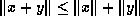 and
and 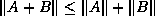 , as well as
  for mutually consistent pairs.
(For more details on the properties of norms, see Golub and
Van Loan
[109].)
for mutually consistent pairs.
(For more details on the properties of norms, see Golub and
Van Loan
[109].)
One difference between these norms is their dependence on dimension.
A vector
of length
with entries uniformly distributed between
0 and 1 will satisfy  , but
will grow
like
, but
will grow
like  and
and  will grow like
. Therefore a stopping
criterion based on
(or
) may have to be permitted to
grow proportional to
(or
) in order that it does not become
much harder to satisfy for large
.
will grow like
. Therefore a stopping
criterion based on
(or
) may have to be permitted to
grow proportional to
(or
) in order that it does not become
much harder to satisfy for large
.
There are two approaches to bounding the
inaccuracy of the computed solution to
.
Since  ,
which we will call the forward error,
is hard to estimate directly,
we introduce
the backward error, which allows us to bound the forward error.
The normwise backward error is defined as
the smallest possible value of
,
which we will call the forward error,
is hard to estimate directly,
we introduce
the backward error, which allows us to bound the forward error.
The normwise backward error is defined as
the smallest possible value of
 where
is the exact solution of
where
is the exact solution of 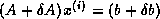 (here
denotes a general matrix, not
times
; the
same goes for
).
The backward error may be easily computed from the residual
; we show how below.
Provided one has
some bound on the inverse of
,
one can bound the forward error in terms of the backward error via
the simple equality
(here
denotes a general matrix, not
times
; the
same goes for
).
The backward error may be easily computed from the residual
; we show how below.
Provided one has
some bound on the inverse of
,
one can bound the forward error in terms of the backward error via
the simple equality

which implies
.
Therefore, a stopping criterion of the form ``stop when  '' also yields an upper bound on the forward error
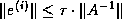 . (Sometimes we may prefer to
use the stricter but harder to estimate bound
. (Sometimes we may prefer to
use the stricter but harder to estimate bound 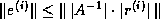 ; see §
. Here
; see §
. Here
 is the matrix or vector of absolute values of components of
 .)
.)
The backward error also has a direct interpretation as a stopping
criterion, in addition to supplying a bound on the forward error.
Recall that the backward error is the smallest change
to the problem
that makes
an exact solution of
. If the original data
and
have
errors from previous computations or measurements,
then it is usually not worth iterating until
and
are even
smaller than these errors.
For example, if the machine precision is
, it is not
worth making  and
and
 , because just rounding the entries
of
and
to fit in the machine creates errors this large.
, because just rounding the entries
of
and
to fit in the machine creates errors this large.
Based on this discussion, we will now consider
some stopping criteria and their
properties. Above we already mentioned
- Criterion 1.
-
 .
This is equivalent to asking that
the backward error
and
described above satisfy
.
This is equivalent to asking that
the backward error
and
described above satisfy
 and
and
 .
This criterion yields the forward error bound
.
This criterion yields the forward error bound

The second stopping criterion we discussed, which does not require
,
may be much more stringent than Criterion 1:
- Criterion 2.
-
 .
This is equivalent to asking that
the backward error
and
satisfy
.
This is equivalent to asking that
the backward error
and
satisfy
 and
and  .
One difficulty with this method is that if
.
One difficulty with this method is that if  ,
which can only occur if
is very ill-conditioned and
nearly
lies in the null space of
,
then it may be difficult
for any method to satisfy the stopping criterion. To see that
must
be very ill-conditioned, note that
,
which can only occur if
is very ill-conditioned and
nearly
lies in the null space of
,
then it may be difficult
for any method to satisfy the stopping criterion. To see that
must
be very ill-conditioned, note that
This criterion yields the forward error bound

If an estimate of
is available, one can also just stop
when the upper bound on the error  falls below
a threshold. This yields the third stopping criterion:
falls below
a threshold. This yields the third stopping criterion:
- Criterion 3.
-
 .
This stopping criterion guarantees that
.
This stopping criterion guarantees that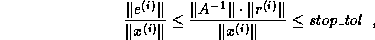
permitting the user to specify the desired relative accuracy stop_tol
in the computed solution
.
One drawback to Criteria 1 and 2 is that they usually treat backward errors in
each component of
and
equally, since most
norms  and
and  measure each entry of
and
equally.
For example, if
is sparse and
is dense, this loss of
possibly important structure will not be reflected in
.
In contrast, the following stopping criterion gives one the option of scaling
each component
measure each entry of
and
equally.
For example, if
is sparse and
is dense, this loss of
possibly important structure will not be reflected in
.
In contrast, the following stopping criterion gives one the option of scaling
each component  and
and  differently,
including the possibility of insisting that some entries be zero.
The cost is an extra matrix-vector multiply:
differently,
including the possibility of insisting that some entries be zero.
The cost is an extra matrix-vector multiply:
- Criterion 4.
-
 .
Here
.
Here  is a user-defined matrix of nonnegative entries,
is a user-defined vector of nonnegative entries, and
is a user-defined matrix of nonnegative entries,
is a user-defined vector of nonnegative entries, and
 denotes the vector of absolute values of the entries of
.
If this criterion is satisfied, it means there are a
and a
such that
, with
denotes the vector of absolute values of the entries of
.
If this criterion is satisfied, it means there are a
and a
such that
, with
 , and
, and
 for all
and
.
By choosing
and
, the user can vary the way
the backward error is measured
in the stopping criterion. For example, choosing
for all
and
.
By choosing
and
, the user can vary the way
the backward error is measured
in the stopping criterion. For example, choosing  and
and  makes the stopping criterion
 ,
which is essentially the same as Criterion 1. Choosing
,
which is essentially the same as Criterion 1. Choosing  and
and
 makes the stopping criterion measure the
componentwise relative backward error, i.e., the smallest relative
perturbations in any component of
and
which is necessary to make
an exact solution. This tighter stopping criterion requires, among other
things, that
have the same sparsity pattern as
.
Other choices of
and
can be used to reflect other structured
uncertainties in
and
.
This criterion yields the forward error bound
makes the stopping criterion measure the
componentwise relative backward error, i.e., the smallest relative
perturbations in any component of
and
which is necessary to make
an exact solution. This tighter stopping criterion requires, among other
things, that
have the same sparsity pattern as
.
Other choices of
and
can be used to reflect other structured
uncertainties in
and
.
This criterion yields the forward error bound
where
is the matrix of absolute values of entries of  .
.
Finally, we mention one more criterion, not because we recommend it,
but because it is widely used. We mention it in order to explain its
potential drawbacks:
- Dubious Criterion 5.
-
 .
This commonly used criterion has the disadvantage of depending too strongly
on the initial solution
.
This commonly used criterion has the disadvantage of depending too strongly
on the initial solution  . If
. If  , a common choice, then
 . Then this criterion is equivalent to Criterion 2 above, which
may be difficult to satisfy for any algorithm
if
. Then this criterion is equivalent to Criterion 2 above, which
may be difficult to satisfy for any algorithm
if  .
On the other hand, if
is very large
and very inaccurate, then
.
On the other hand, if
is very large
and very inaccurate, then  will be very large and
  will be
artificially large; this means the iteration may stop too soon.
This criterion yields the forward error bound
will be
artificially large; this means the iteration may stop too soon.
This criterion yields the forward error bound
 .
.
Next:
When or is
Up:
Stopping Criteria
Previous:
Stopping Criteria
Jack Dongarra
Mon Nov 20 08:52:54 EST 1995
When <IMG ALIGN=BOTTOM SRC="http://www.netlib.org/utk/papers/templates/_22900_tex2html_wrap6695.gif">
or <IMG ALIGN=BOTTOM SRC="http://www.netlib.org/utk/papers/templates/_22900_tex2html_wrap6959.gif">
is not readily available
Next:
Estimating
Up:
Stopping Criteria
Previous:
More Details about
It is possible to design an iterative algorithm for which
or
is not directly available,
although this is not the case for any algorithms in this book.
For completeness, however, we discuss stopping criteria in this case.
For example, if ones ``splits''
to get the iterative
method  , then the
natural residual to compute is
, then the
natural residual to compute is
 .
In other words, the residual
.
In other words, the residual  is the same as the residual of the
preconditioned system
is the same as the residual of the
preconditioned system  . In this case, it is
hard to interpret
as a backward error for the original system
, so we may instead derive a forward error bound
. In this case, it is
hard to interpret
as a backward error for the original system
, so we may instead derive a forward error bound
 .
Using this as a stopping criterion requires an estimate of
.
Using this as a stopping criterion requires an estimate of
 .
In the case of methods based on
splitting
, we have
.
In the case of methods based on
splitting
, we have  ,
and
,
and  .
.
Another example is an implementation of the preconditioned conjugate
gradient algorithm which computes  instead of
(the
implementation in this book computes the latter). Such an
implementation could use the stopping criterion
instead of
(the
implementation in this book computes the latter). Such an
implementation could use the stopping criterion  as in Criterion 5. We
may also use it to get the forward error bound
as in Criterion 5. We
may also use it to get the forward error bound  , which could also
be used in a stopping criterion.
, which could also
be used in a stopping criterion.
Jack Dongarra
Mon Nov 20 08:52:54 EST 1995
Estimating <IMG ALIGN=BOTTOM SRC="http://www.netlib.org/utk/papers/templates/_22900_tex2html_wrap6665.gif">
Next:
Stopping when progress
Up:
Stopping Criteria
Previous:
When or is
Bounds on the error
inevitably rely on bounds for
,
since  . There is a large number of problem dependent
ways to estimate
; we mention a few here.
. There is a large number of problem dependent
ways to estimate
; we mention a few here.
When a splitting
is used to get an iteration

then the matrix whose
inverse norm we need is  . Often, we know how to estimate
 if the splitting is a standard one such as Jacobi or SOR,
and the matrix
has special characteristics such as Property A.
Then we may estimate
if the splitting is a standard one such as Jacobi or SOR,
and the matrix
has special characteristics such as Property A.
Then we may estimate  .
.
When
is symmetric positive definite, and Chebyshev acceleration with
adaptation of parameters is being used, then at each step the algorithm
estimates the largest and smallest eigenvalues  and
and
 of
anyway.
Since
is symmetric positive definite,
of
anyway.
Since
is symmetric positive definite,
 .
.
This adaptive estimation is often done using the Lanczos algorithm
(see section
),
which can usually provide good estimates of the
largest (rightmost) and smallest (leftmost) eigenvalues of a symmetric matrix
at the cost of a few matrix-vector multiplies.
For general nonsymmetric
, we may apply
the Lanczos method to
or
,
and use the fact that
 .
.
It is also possible to estimate  provided one is willing
to solve a few systems of linear equations with
and
as coefficient
matrices. This is often done with dense linear system solvers, because the
extra cost of these systems is
provided one is willing
to solve a few systems of linear equations with
and
as coefficient
matrices. This is often done with dense linear system solvers, because the
extra cost of these systems is  , which is small compared to the cost
 of the LU decomposition (see Hager
[121],
Higham
[124] and Anderson, et al.
[3]).
This is not the case for iterative solvers, where the cost of these
solves may well be several times as much as the original linear system.
Still, if many linear systems with the same coefficient matrix and
differing right-hand-sides are to be solved, it is a viable method.
of the LU decomposition (see Hager
[121],
Higham
[124] and Anderson, et al.
[3]).
This is not the case for iterative solvers, where the cost of these
solves may well be several times as much as the original linear system.
Still, if many linear systems with the same coefficient matrix and
differing right-hand-sides are to be solved, it is a viable method.
The approach in the last paragraph also lets us estimate the alternate
error bound  .
This may be much smaller than the simpler
.
This may be much smaller than the simpler
 in the
case where the rows of
are badly scaled; consider the case of a
diagonal matrix
with widely varying diagonal entries. To
compute
in the
case where the rows of
are badly scaled; consider the case of a
diagonal matrix
with widely varying diagonal entries. To
compute  , let
, let  denote the diagonal
matrix with diagonal entries equal to the entries of
; then
denote the diagonal
matrix with diagonal entries equal to the entries of
; then
 (see Arioli, Demmel and Duff
[5]).
(see Arioli, Demmel and Duff
[5]).  can be estimated using the
technique in the last paragraph since multiplying by
can be estimated using the
technique in the last paragraph since multiplying by
 or
or  is no harder than multiplying
by
and
is no harder than multiplying
by
and  and also by
, a diagonal matrix.
and also by
, a diagonal matrix.
Next:
Stopping when progress
Up:
Stopping Criteria
Previous:
When or is
Jack Dongarra
Mon Nov 20 08:52:54 EST 1995
Stopping when progress is no longer being made
Next:
Accounting for floating
Up:
Stopping Criteria
Previous:
Estimating
In addition to limiting the total amount of work by limiting the
maximum number of iterations one is willing to do, it is also natural
to consider stopping when no apparent progress is being made.
Some methods, such as Jacobi and SOR, often exhibit nearly monotone
linear convergence, at least after some initial transients, so it
is easy to recognize when convergence degrades. Other methods, like
the conjugate gradient method, exhibit ``plateaus'' in their convergence,
with the residual norm stagnating at a constant value for many iterations
before decreasing again; in principle there can be many such plateaus
(see Greenbaum and Strakos
[110]) depending on the problem.
Still other methods, such as CGS, can appear
wildly nonconvergent for a large number of steps before the residual begins
to decrease; convergence may continue to be erratic from step to step.
In other words, while it is a good idea to have a criterion that stops
when progress towards a solution is no longer being made, the
form of such a criterion is both method and problem dependent.
Jack Dongarra
Mon Nov 20 08:52:54 EST 1995
Accounting for floating point errors
Next:
Data Structures
Up:
Stopping Criteria
Previous:
Stopping when progress
The error bounds discussed in this section are subject to floating
point errors, most of which are innocuous, but which deserve some discussion.
The infinity norm  requires the fewest
floating point operations to compute, and cannot overflow or cause other
exceptions if the
requires the fewest
floating point operations to compute, and cannot overflow or cause other
exceptions if the  are themselves finite
. On the other hand, computing
are themselves finite
. On the other hand, computing
 in the most straightforward manner
can easily overflow or lose accuracy to underflow even when the true result
is far from either the overflow or underflow thresholds. For this reason,
a careful implementation for computing
without this danger
is available (subroutine snrm2 in the BLAS
[72]
[144]),
but it is more expensive than computing
in the most straightforward manner
can easily overflow or lose accuracy to underflow even when the true result
is far from either the overflow or underflow thresholds. For this reason,
a careful implementation for computing
without this danger
is available (subroutine snrm2 in the BLAS
[72]
[144]),
but it is more expensive than computing  .
.
Now consider computing the residual
by forming the
matrix-vector product  and then subtracting
, all in floating
point arithmetic with relative precision
. A standard error
analysis shows that the error
and then subtracting
, all in floating
point arithmetic with relative precision
. A standard error
analysis shows that the error  in the computed
is bounded by
in the computed
is bounded by
 , where
 is typically bounded by
  , and
usually closer to
, and
usually closer to  . This is why one should not choose
 in Criterion 1, and why Criterion 2 may not
be satisfied by any method.
This uncertainty in the value of
induces an uncertainty in the error
of
at most
in Criterion 1, and why Criterion 2 may not
be satisfied by any method.
This uncertainty in the value of
induces an uncertainty in the error
of
at most
 .
A more refined bound is that the error
.
A more refined bound is that the error  in the
th component of
is bounded by
times the
th component of
in the
th component of
is bounded by
times the
th component of
 , or more tersely
.
This means the uncertainty in
is really bounded by
, or more tersely
.
This means the uncertainty in
is really bounded by
 .
This last quantity can be estimated inexpensively provided solving systems
with
and
as coefficient matrices is inexpensive (see the last
paragraph of §
).
Both these bounds can be severe overestimates of the uncertainty in
,
but examples exist where they are attainable.
.
This last quantity can be estimated inexpensively provided solving systems
with
and
as coefficient matrices is inexpensive (see the last
paragraph of §
).
Both these bounds can be severe overestimates of the uncertainty in
,
but examples exist where they are attainable.
Next:
Data Structures
Up:
Stopping Criteria
Previous:
Stopping when progress
Jack Dongarra
Mon Nov 20 08:52:54 EST 1995
Data Structures
Next:
Survey of Sparse
Up:
Related Issues
Previous:
Accounting for floating
The efficiency of any of the iterative methods considered in previous
sections is determined primarily by the performance of the
matrix-vector product and the preconditioner solve, and therefore on
the storage scheme used for the matrix and the preconditioner. Since
iterative methods are typically used on sparse matrices, we will
review here a number of sparse storage formats.
Often, the storage scheme used
arises naturally from the specific application problem.
Storage scheme: The way elements of a matrix are stored
in the memory of a computer. For dense matrices, this can be
the decision to store rows or columns consecutively.
For sparse matrices, common storage schemes avoid storing zero elements;
as a result they involve integer data describing where the stored elements
fit into the global matrix.
In this section we will review some of the more popular sparse matrix
formats that are used in numerical software packages such as ITPACK
[140] and NSPCG
[165].
After surveying the various formats, we demonstrate how the
matrix-vector product and an incomplete factorization solve are
formulated using two of the sparse matrix formats.
Jack Dongarra
Mon Nov 20 08:52:54 EST 1995
Iterative Methods
Next:
Overview of the
Up:
Templates for the Solution
Previous:
What Methods Are
The term ``iterative method'' refers to a wide range of techniques
that use successive approximations to obtain more accurate solutions
to a linear system at each step. In this book we will cover two types
of iterative methods.
Stationary methods are older, simpler to understand
and implement, but usually not as effective.
Nonstationary methods are a relatively recent
development; their analysis is usually harder to understand, but they
can be highly effective. The nonstationary methods we present are
based on the idea of sequences of orthogonal vectors. (An exception
is the Chebyshev
iteration method, which is based on
orthogonal polynomials.)
Stationary iterative method: Iterative method that performs
in each iteration the same operations on the current iteration vectors.
Nonstationary iterative method: Iterative method that
has iteration-dependent coefficients.
Dense matrix: Matrix for which the number of zero elements
is too small to warrant specialized algorithms.
Sparse matrix: Matrix for which the number of zero elements
is large enough that algorithms avoiding operations on zero elements
pay off. Matrices derived from partial differential equations typically
have a number of nonzero elements that is proportional to the matrix size,
while the total number of matrix elements is the square of the matrix size.
The rate at which an iterative method converges depends greatly on the
spectrum of the coefficient matrix. Hence, iterative methods usually
involve a second matrix that transforms the coefficient matrix into
one with a more favorable spectrum. The transformation matrix is
called a preconditioner.
A good preconditioner improves the convergence of the iterative method,
sufficiently to overcome the extra cost of constructing and applying
the preconditioner. Indeed, without a preconditioner the iterative
method may even fail to converge.
Jack Dongarra
Mon Nov 20 08:52:54 EST 1995
Survey of Sparse Matrix Storage Formats
Next:
Compressed Row Storage
Up:
Data Structures
Previous:
Data Structures
If the coefficient matrix
is sparse, large-scale linear systems
of the form
can be most
efficiently solved if the
zero elements of
are not stored. Sparse storage schemes allocate
contiguous storage in memory for
the nonzero elements of the matrix, and perhaps a limited number of
zeros. This, of course, requires a scheme for knowing
where the elements fit into the full matrix.
There are many methods for
storing the data (see for instance Saad
[186]
and Eijkhout
[87]).
Here we will discuss Compressed Row and Column Storage, Block Compressed
Row Storage, Diagonal Storage, Jagged Diagonal Storage, and Skyline
Storage.
Jack Dongarra
Mon Nov 20 08:52:54 EST 1995
Compressed Row Storage (CRS)
Next:
Compressed Column Storage
Up:
Survey of Sparse
Previous:
Survey of Sparse
The Compressed Row and Column (in the next section) Storage formats
are the most general: they make absolutely no assumptions about the
sparsity structure of the matrix, and they don't store any unnecessary
elements. On the other hand, they are not very efficient, needing an
indirect addressing step for every single scalar operation in a matrix-vector
product or preconditioner solve.
The Compressed Row Storage (CRS) format puts the subsequent nonzeros of the
matrix rows in contiguous memory locations.
Assuming we have a nonsymmetric sparse matrix
, we create
vectors:
one for floating-point numbers (val), and the other two for
integers (col_ind, row_ptr). The val vector
stores the values of the nonzero elements of the
matrix
, as they are traversed in a row-wise fashion.
The col_ind vector stores
the column indexes of the elements in the val vector.
That is, if  then
then  .
The row_ptr vector stores
the locations in the val vector that start a row, that is,
if
then
.
The row_ptr vector stores
the locations in the val vector that start a row, that is,
if
then  .
By convention, we define
.
By convention, we define  , where
  is
the number of nonzeros in the matrix
. The storage savings for this
approach is significant. Instead of storing
is
the number of nonzeros in the matrix
. The storage savings for this
approach is significant. Instead of storing  elements,
we need only
elements,
we need only  storage locations.
As an example, consider the nonsymmetric matrix
defined by
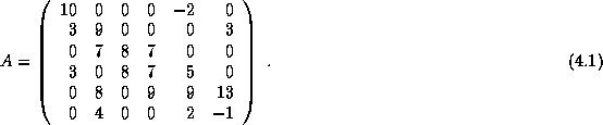
The CRS format for this matrix is then specified by the arrays
{val, col_ind, row_ptr} given below


.
If the matrix
is symmetric, we need only store the upper (or
lower) triangular portion of the matrix. The trade-off is
a more complicated algorithm with a somewhat different pattern of data access.
Jack Dongarra
Mon Nov 20 08:52:54 EST 1995
Compressed Column Storage (CCS)
Next:
Block Compressed Row
Up:
Survey of Sparse
Previous:
Compressed Row Storage
Analogous to Compressed Row Storage there is Compressed Column
Storage (CCS), which is also called the Harwell-Boeing
sparse matrix format
[78]. The CCS format is identical to the
CRS format except that the columns of
are stored (traversed) instead
of the rows. In other words, the CCS format is the CRS format
for
.
The CCS format is specified by the
arrays
{val, row_ind, col_ptr}, where
row_ind stores the row indices of each nonzero, and col_ptr
stores the index of the elements in val which start a column of
.
The CCS format for the matrix
in (
) is
given by


.
Jack Dongarra
Mon Nov 20 08:52:54 EST 1995
Block Compressed Row Storage (BCRS)
Next:
Compressed Diagonal Storage
Up:
Survey of Sparse
Previous:
Compressed Column Storage
If the sparse matrix
is comprised of square
dense blocks of nonzeros in some regular pattern, we can modify
the CRS (or CCS) format to exploit such block patterns. Block
matrices typically arise from the discretization of partial differential
equations in which there are several degrees of freedom associated
with a grid point. We then partition the matrix in small blocks with
a size equal to the number of degrees of freedom, and treat each
block as a dense matrix, even though it may have some zeros.
If
is the dimension of each block and  is the number of nonzero
blocks in the
matrix
, then the total storage
needed is
is the number of nonzero
blocks in the
matrix
, then the total storage
needed is  .
The block
dimension
.
The block
dimension  of
is then defined by
of
is then defined by  .
.
Similar to the CRS format, we require
arrays for the BCRS format:
a rectangular array for floating-point numbers (
val( ,
, ,
)) which stores the nonzero blocks in
(block) row-wise fashion, an integer array (col_ind(
))
which stores the actual column indices in the original matrix
of
the (
,
)) which stores the nonzero blocks in
(block) row-wise fashion, an integer array (col_ind(
))
which stores the actual column indices in the original matrix
of
the ( ) elements of the nonzero blocks, and a pointer
array (row_blk(
) elements of the nonzero blocks, and a pointer
array (row_blk( )) whose entries point to the beginning of
each block row in val(:,:,:) and col_ind(:). The
savings in storage locations and reduction in indirect addressing for
BCRS over CRS can be significant for matrices with a large
.
)) whose entries point to the beginning of
each block row in val(:,:,:) and col_ind(:). The
savings in storage locations and reduction in indirect addressing for
BCRS over CRS can be significant for matrices with a large
.
Jack Dongarra
Mon Nov 20 08:52:54 EST 1995
Compressed Diagonal Storage (CDS)
Next:
Jagged Diagonal Storage
Up:
Survey of Sparse
Previous:
Block Compressed Row
If the matrix
is banded with bandwidth that is fairly constant
from row to row,
then it is worthwhile to take advantage of this
structure in the storage scheme by storing subdiagonals of the matrix
in consecutive locations. Not only can we eliminate the vector
identifying the column and row, we can pack the nonzero elements in such a
way as to make the matrix-vector product more efficient.
This storage scheme is particularly useful if the matrix arises from
a finite element or finite difference discretization on a tensor
product grid.
We say that the matrix  is
banded if there are nonnegative constants
,
, called the left and
right halfbandwidth, such
that
only if
is
banded if there are nonnegative constants
,
, called the left and
right halfbandwidth, such
that
only if  . In this case, we can
allocate for the matrix
an array val(1:n,-p:q).
The declaration with reversed dimensions (-p:q,n) corresponds to the
LINPACK band format
[73], which unlike CDS,
does not allow for an
efficiently vectorizable matrix-vector multiplication if
. In this case, we can
allocate for the matrix
an array val(1:n,-p:q).
The declaration with reversed dimensions (-p:q,n) corresponds to the
LINPACK band format
[73], which unlike CDS,
does not allow for an
efficiently vectorizable matrix-vector multiplication if  is small.
Usually, band formats involve storing some zeros. The CDS
format may even contain some array elements that do not
correspond to matrix elements at all.
Consider the nonsymmetric matrix
defined by
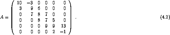
Using the CDS format, we
store this matrix
in an array of dimension (6,-1:1) using
the mapping

Hence, the rows of the val(:,:) array are
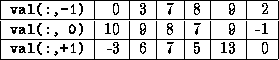
.
Notice the two zeros corresponding to non-existing matrix elements.
A generalization of the CDS format more suitable for manipulating
general sparse matrices on vector supercomputers is discussed by
Melhem in
[154]. This variant of CDS uses a stripe data structure to store the matrix
. This structure is
more efficient in storage in the case of varying bandwidth, but it
makes the matrix-vector product slightly more expensive, as it
involves a gather operation.
As defined in
[154],
a stripe in the
matrix
is a set of positions
 , where
  and
and  is a strictly increasing function.
Specifically, if
is a strictly increasing function.
Specifically, if  and
and  are in
,
then
are in
,
then

When computing the
matrix-vector product  using stripes, each
 element of
in stripe
element of
in stripe  is multiplied
with both
and
is multiplied
with both
and  and these products are
accumulated in
and these products are
accumulated in  and
and  , respectively. For
the nonsymmetric matrix
defined by
, respectively. For
the nonsymmetric matrix
defined by
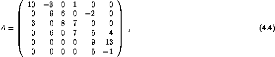
the
stripes of the matrix
stored
in the rows of the val(:,:) array would be
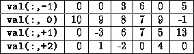
.
Next:
Jagged Diagonal Storage
Up:
Survey of Sparse
Previous:
Block Compressed Row
Jack Dongarra
Mon Nov 20 08:52:54 EST 1995
Jagged Diagonal Storage (JDS)
Next:
Skyline Storage (SKS)
Up:
Survey of Sparse
Previous:
Compressed Diagonal Storage
The Jagged Diagonal Storage format can be useful for the
implementation of iterative methods on parallel and vector processors
(see Saad
[185]). Like the Compressed Diagonal
format, it gives a vector length essentially of the size of the
matrix. It is more space-efficient than CDS at the cost of a
gather/scatter operation.
A simplified form of JDS, called ITPACK storage or Purdue
storage, can be described as follows. In the matrix
from (
) all elements are shifted left:
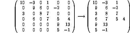
after which the columns are stored consecutively. All rows are padded
with zeros on the right to give them equal length. Corresponding to
the array of matrix elements val(:,:),
an array of column indices, col_ind(:,:) is also stored:
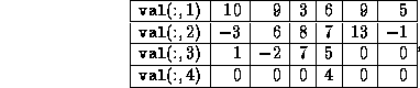
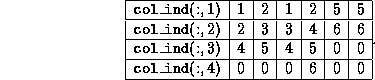
It is clear that the padding zeros in this structure may be a
disadvantage, especially if the bandwidth of the matrix varies strongly.
Therefore, in the CRS format, we
reorder the rows of the matrix decreasingly according to
the number of nonzeros per row. The compressed and permuted diagonals
are then stored in a linear array. The new data structure is called
jagged diagonals.
The number of jagged diagonals is equal to
the number of nonzeros in the first row, i.e., the largest
number of nonzeros in any row of
. The data structure to
represent the
matrix
therefore consists of a permutation
array (perm(1:n)) which reorders the rows, a floating-point array
(jdiag(:)) containing the jagged diagonals in succession,
an integer array (col_ind(:)) containing the corresponding column
indices, and finally a pointer array (jd_ptr(:)) whose elements
point to the beginning of each jagged diagonal. The advantages
of JDS for matrix multiplications are discussed by Saad in
[185].
The JDS format for the above matrix
in using the linear arrays
{perm, jdiag, col_ind, jd_ptr}
is given below (jagged diagonals are separated by semicolons)


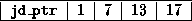
.
Next:
Skyline Storage (SKS)
Up:
Survey of Sparse
Previous:
Compressed Diagonal Storage
Jack Dongarra
Mon Nov 20 08:52:54 EST 1995
Skyline Storage (SKS)
Next:
Matrix vector products
Up:
Survey of Sparse
Previous:
Jagged Diagonal Storage
The final storage scheme we consider is for skyline matrices, which
are also called variable band or profile matrices (see Duff, Erisman
and Reid
[80]). It is mostly of importance in direct solution
methods, but it can be used for handling the diagonal blocks in block
matrix factorization methods. A major advantage of solving linear
systems having skyline coefficient matrices is that when pivoting is
not necessary, the skyline structure is preserved during Gaussian
elimination. If the matrix is symmetric, we only store its lower
triangular part. A straightforward approach in storing the elements
of a skyline matrix is to place all the rows (in order) into a
floating-point array (val(:)), and then keep an integer array
(row_ptr(:)) whose elements point to the beginning of each row.
The column indices of the nonzeros stored in val(:) are easily
derived and are not stored.
For a nonsymmetric skyline matrix such as the one illustrated in
Figure
, we store the lower
triangular elements in SKS format, and store the upper triangular
elements in a column-oriented SKS format (transpose stored in row-wise
SKS format). These two separated substructures can be linked in
a variety of ways. One approach, discussed by Saad
in
[186], is to store each row of the lower triangular
part and each column of the upper triangular part contiguously into
the floating-point array (val(:)). An additional pointer is
then needed to determine where the diagonal elements, which separate
the lower triangular elements from the upper triangular elements, are
located.
Figure: Profile of a nonsymmetric skyline or variable-band
matrix.
Jack Dongarra
Mon Nov 20 08:52:54 EST 1995
Matrix vector products
Next:
CRS Matrix-Vector Product
Up:
Data Structures
Previous:
Skyline Storage (SKS)
In many of the iterative methods discussed earlier, both the product
of a matrix and that of its transpose times a vector are needed, that
is, given an input vector
we want to compute products

We will present
these algorithms for two of the storage formats
from §
: CRS and CDS.
Jack Dongarra
Mon Nov 20 08:52:54 EST 1995
CRS Matrix-Vector Product
Next:
CDS Matrix-Vector Product
Up:
Matrix vector products
Previous:
Matrix vector products
The matrix vector product
using CRS format can be
expressed in the usual way:
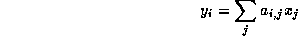
since this traverses the rows of the matrix
.
For an
matrix A, the
matrix-vector multiplication is given by
for i = 1, n
    y(i)  = 0
    for j = row_ptr(i), row_ptr(i+1) - 1
        y(i) = y(i) + val(j) * x(col_ind(j))
    end;
end;
Since this method only multiplies nonzero matrix entries, the
operation count is
times the number of nonzero elements in
,
which is a significant savings over the dense operation requirement
of  .
.
For the transpose product  we cannot use the equation
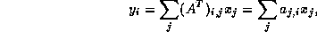
since this implies
traversing columns of the matrix, an extremely inefficient operation
for matrices stored in CRS format. Hence, we switch indices to

The matrix-vector multiplication involving
is then given by
for i = 1, n
    y(i) =  0
end;
for j = 1, n
    for i = row_ptr(j), row_ptr(j+1)-1
        y(col_ind(i)) = y(col_ind(i)) + val(i) * x(j)
    end;
end;
Both matrix-vector products above have largely the same structure, and
both use indirect addressing. Hence, their vectorizability properties
are the same on any given computer. However, the first product
(
) has a more favorable memory access pattern in that (per
iteration of the outer loop) it reads two vectors of data (a row of
matrix
and the input vector
) and writes one scalar. The
transpose product (
) on the other hand reads one element of
the input vector, one row of matrix
, and both reads and writes the
result vector
. Unless the machine on which these methods are
implemented has three separate memory paths (e.g., Cray Y-MP), the
memory traffic will then limit the performance. This is an
important consideration for RISC-based architectures.
Jack Dongarra
Mon Nov 20 08:52:54 EST 1995
CDS Matrix-Vector Product
Next:
Sparse Incomplete Factorizations
Up:
Matrix vector products
Previous:
CRS Matrix-Vector Product
If the
matrix
is
stored in CDS format, it is still possible to
perform a matrix-vector product
by either rows or columns, but this
does not take advantage of the CDS format. The idea
is to make a change in coordinates in the doubly-nested loop. Replacing
 we get

With the index
in the inner loop we see that the
expression  accesses the
th diagonal of the matrix
(where the main diagonal has number 0).
accesses the
th diagonal of the matrix
(where the main diagonal has number 0).
The algorithm will now have a doubly-nested loop with the outer loop
enumerating the diagonals diag=-p,q with
and
the
(nonnegative) numbers of diagonals to the left and right of the main
diagonal. The bounds for the inner loop follow from the requirement
that

The algorithm becomes
for i = 1, n
    y(i) = 0
end;
for diag = -diag_left, diag_right
    for loc = max(1,1-diag), min(n,n-diag)
        y(loc) = y(loc) + val(loc,diag) * x(loc+diag)
    end;
end;
The transpose matrix-vector product
is a minor variation of the
algorithm above. Using the update formula

we obtain
for i = 1, n
    y(i) = 0
end;
for diag = -diag_right, diag_left
    for loc = max(1,1-diag), min(n,n-diag)
        y(loc) = y(loc) + val(loc+diag, -diag) * x(loc+diag)
    end;
end;
The memory access for the CDS-based matrix-vector product
(or
) is
three vectors per inner iteration. On the other hand, there is no
indirect addressing, and the algorithm is vectorizable with vector
lengths of essentially the matrix order
. Because of the regular data
access, most machines can perform this algorithm
efficiently by keeping three base registers and using simple offset
addressing.
Jack Dongarra
Mon Nov 20 08:52:54 EST 1995
Templates for the Solution of Linear Systems: <BR>Building Blocks for Iterative Methods<A NAME=tex2html1 HREF="http://www.netlib.org/utk/papers/templates/footnode.html#22">
<IMG ALIGN=BOTTOM ALT="gif" SRC="http://www.netlib.org/utk/icons/foot_motif.gif">
</A>


Next:
How to Use
=25pt
-8pt
Eijk-hout
Templates for the Solution of Linear Systems:
Building Blocks for Iterative Methods
Richard Barrett
,Michael Berry
,
Tony F. Chan
,
James Demmel
,
June M. Donato
,
Jack Dongarra  ,
,
Victor Eijkhout ,
Roldan Pozo
Charles Romine ,
and
Henk Van der Vorst
This book is also available in Postscript from over the Internet.
To retrieve the postscript file you can use one of the following methods:
-
anonymous ftp to www.netlib.org
cd templates
get templates.ps
quit
-
from any machine on the Internet type:
rcp anon@www.netlib.org:templates/templates.ps templates.ps
-
send email to netlib@ornl.gov and in the message type:
send templates.ps from templates
The url for this book is
http://www.netlib.org/templates/Templates.html .
A bibtex reference for this book follows:
@BOOK{templates,
AUTHOR = {R. Barrett and M. Berry and T. F. Chan and J. Demmel and
J. Donato and J. Dongarra and V. Eijkhout and R. Pozo and
C. Romine, and H. Van der Vorst },
TITLE = {Templates for the Solution of Linear Systems:
Building Blocks for Iterative Methods},
PUBLISHER = {SIAM},
YEAR = {1994},
ADDRESS = {Philadelphia, PA} }
Jack Dongarra
Mon Nov 20 08:52:54 EST 1995