


Next: Nonlinear Eigenvalue Problems with
Up: Nonlinear Eigenvalue Problems
Previous: Notes and References
Contents
Index
Higher Order Polynomial Eigenvalue Problems
Some applications lead to a higher order polynomial eigenvalue problem (PEP)
 |
(268) |
where  is a matrix polynomial defined as
in which the  are square
  by matrices.
A thorough study of the mathematical properties of matrix polynomials
can be found in [194].
by matrices.
A thorough study of the mathematical properties of matrix polynomials
can be found in [194].
In order to make the eigenvalue
problem well defined, these matrices have to satisfy certain properties;
in particular  should be nonsingular.
Similar to the quadratic problem, these problems can also be linearized
to
should be nonsingular.
Similar to the quadratic problem, these problems can also be linearized
to
where
The relation between  and
and  is given by
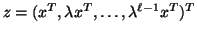 .
.
 is a block companion matrix of the PEP.
The generalized
eigenproblem
is a block companion matrix of the PEP.
The generalized
eigenproblem  can be solved with one of the methods
discussed in Chapter 8.
A disadvantage of this approach is that one
has to work with larger matrices of order
can be solved with one of the methods
discussed in Chapter 8.
A disadvantage of this approach is that one
has to work with larger matrices of order  , and these matrices
also have eigenpairs, of course. This implies that one has to
check which of the computed eigenpairs satisfies the original polynomial
equation.
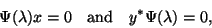
Ruhe [372] (see also Davis [102]) discussed methods that
directly handle the problem
(9.24), for instance, with Newton's method. For larger values
of one may expect all sorts of problems with the convergence of these
techniques.
In §9.2.5, we have discussed a method that can be used
to attack problems with large . In that approach, one first projects
the given problem (9.24) onto a low-dimensional subspace and
obtains a similar problem of low dimension. This low-dimensional polynomial
eigenproblem can then be solved with one of the approaches mentioned
above. In [221] a fourth-order polynomial problem has been solved
successfully, using this reduction technique.
, and these matrices
also have eigenpairs, of course. This implies that one has to
check which of the computed eigenpairs satisfies the original polynomial
equation.
Ruhe [372] (see also Davis [102]) discussed methods that
directly handle the problem
(9.24), for instance, with Newton's method. For larger values
of one may expect all sorts of problems with the convergence of these
techniques.
In §9.2.5, we have discussed a method that can be used
to attack problems with large . In that approach, one first projects
the given problem (9.24) onto a low-dimensional subspace and
obtains a similar problem of low dimension. This low-dimensional polynomial
eigenproblem can then be solved with one of the approaches mentioned
above. In [221] a fourth-order polynomial problem has been solved
successfully, using this reduction technique.
Next: Nonlinear Eigenvalue Problems with
Up: Nonlinear Eigenvalue Problems
Previous: Notes and References
Contents
Index
Susan Blackford
2000-11-20
![\begin{displaymath}
A \equiv \left[ \begin{array}{ccccc}
0 & I & 0 & \cdots & 0 ...
...& \\
& & & I & \\
& & & & C_\ell \\
\end{array} \right] .
\end{displaymath}](img3400.png)