


Next: Error Bound for Computed
Up: Stability and Accuracy Assessments
Previous: Residual Vectors.
Contents
Index
Transfer Residual Errors to Backward Errors.
It turns out that the computed
eigenvalue and eigenvector(s) can always be interpreted as
the exact one of nearby matrices, i.e.,
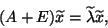
and
if  is available,
where the error matrices
is available,
where the error matrices  are generally small in norm
relative to
are generally small in norm
relative to  . Such an interpretation
serves two purposes: first, it reflects indirectly how accurately
the eigenproblem has been solved; and second, it can be used to derive
error bounds for the computed eigenvalues and eigenvectors to be
discussed below. Ideally, we would like to be zero
matrices, but this hardly ever happens at all in practice. There are infinitely
many error matrices that satisfy the above equations,
we would like to know only the optimal or nearly
optimal error matrices in the sense that certain norms (usually the
2-norm
. Such an interpretation
serves two purposes: first, it reflects indirectly how accurately
the eigenproblem has been solved; and second, it can be used to derive
error bounds for the computed eigenvalues and eigenvectors to be
discussed below. Ideally, we would like to be zero
matrices, but this hardly ever happens at all in practice. There are infinitely
many error matrices that satisfy the above equations,
we would like to know only the optimal or nearly
optimal error matrices in the sense that certain norms (usually the
2-norm  or the Frobenius norm
  ) are
minimized among all feasible error matrices. In fact, practical purposes
will be served if we can determine upper bounds for the norms of these
(nearly)
optimal matrices. The following collection of results indeed shows that
if
) are
minimized among all feasible error matrices. In fact, practical purposes
will be served if we can determine upper bounds for the norms of these
(nearly)
optimal matrices. The following collection of results indeed shows that
if  (and
(and  if available) is small, the
error matrix is small, too [425].
if available) is small, the
error matrix is small, too [425].
We distinguish two cases.
- Only
 is available but is not. Then
the optimal error matrix (in both 2-norm
and the Frobenius norm) for which
is available but is not. Then
the optimal error matrix (in both 2-norm
and the Frobenius norm) for which  and are
an exact eigenvalue and its corresponding eigenvector of
and are
an exact eigenvalue and its corresponding eigenvector of  , i.e.,
 |
(210) |
satisfies
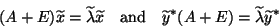
- Both and are available. Then
the optimal error matrices
 (in 2-norm) and
  (in the Frobenius norm) for which , , and
are
an exact eigenvalue and its corresponding eigenvectors of , i.e.,
(in the Frobenius norm) for which , , and
are
an exact eigenvalue and its corresponding eigenvectors of , i.e.,
 |
(211) |
for  , satisfy
and
See [256,431].
We say the algorithm
that delivers the approximate eigenpair
 is
is
 -backward stable
for the pair with respect to the norm
-backward stable
for the pair with respect to the norm  if it is an exact eigenpair for with
  ; analogously
the algorithm that delivers the eigentriplet
; analogously
the algorithm that delivers the eigentriplet
 is -backward stable for the triplet with respect to the norm
if it is an exact eigentriplet for with .
With these in mind,
statements can be made about the backward stability of the algorithm which
computes the eigenpair
or
the eigentriplet
.
Conventionally, an algorithm is called backward stable
if
is -backward stable for the triplet with respect to the norm
if it is an exact eigentriplet for with .
With these in mind,
statements can be made about the backward stability of the algorithm which
computes the eigenpair
or
the eigentriplet
.
Conventionally, an algorithm is called backward stable
if
 .
.
Next: Error Bound for Computed
Up: Stability and Accuracy Assessments
Previous: Residual Vectors.
Contents
Index
Susan Blackford
2000-11-20