Jacobi-Davidson Methods
 G. Sleijpen and H. van der Vorst

We consider the application of the Jacobi-Davidson approach to the GHEP (5.1). We can, similarly as for the Lanczos method treated in the previous section (see also [444]), apply the Jacobi-Davidson method to (5.1), with a $B$-orthogonal basis ${v}_1,{v}_2,\ldots , {v}_{m}$ for the search subspace; that is,

$${V}_{m}^\ast B{V}_{m}=I_{m},$$

if we let ${V}_{m}$ denote the matrix with columns ${v}_j$.

The Ritz-Galerkin condition for vectors ${u}\equiv {V}_{m}{s}$ in this subspace leads to

$$({V}_{m}^\ast A {V}_{m}) {s} - \theta ({V}_{m}^\ast B {V}_{m}) {s} = 0 ,$$ (88)

or, because of the $B$-orthogonality of ${V}_{m}$:

$$({V}_{m}^\ast A {V}_{m}) {s} - \theta {s} = 0 .$$

This leads to Ritz vectors ${u}_j^{(m)}\equiv V_{m}{s}_j$ and Ritz values $\theta_j^{(m)}$. We will assume that these Ritz vectors are normalized with respect to the $B$-inner product.

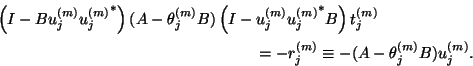
The correction equation for the eigenvector component $t_j^{({m})}\perp B{u}_j^{(m)}$ for the generalized eigenproblem can be written as

$$\begin{array}{r} \left( I - B{u}_j^{(m)} {{u}_j^{(m)}}^\ast... ...j^{({m})}\equiv - (A-\theta_j^{(m)} B){u}_j^{(m)} . \end{array}$$ (89)

If linear systems with the matrix $A-\theta_j^{(m)} B$ are efficiently solvable, then we can compute the exact solution $t_j^{({m})}$. In other cases we can, as is usual for the Jacobi-Davidson methods, compute approximate solutions to $t_j^{({m})}$ with a Krylov solver applied to (5.25). Note that the operator

$$\left( I - B{u}_j^{(m)} {{u}_j^{(m)}}^\ast \right) (A-\theta_j^{(m)} B) \left( I - {u}_j^{(m)} {{u}_j^{(m)}}^\ast B \right)$$

maps the space $(B{u}_j^{(m)})^\perp$ onto the space $({u}_j^{(m)})^\perp$, so that preconditioning is always required if we use a Krylov solver in order to get a mapping between $(B{u}_j^{(m)})^\perp$ and $(B{u}_j^{(m)})^\perp$ (see item (31) of Algorithm 5.6).

As for the standard Hermitian case, the resulting scheme can be combined with restart and deflation. If we want to work with orthogonal operators in the deflation, then we have to work with $B$-orthogonal matrices that reduce the given generalized system to Schur form:

$$A{Q}_{k}={Z}_{k}{D}_{k},$$

in which ${Z}_{k}=B{Q}_{k}$ and ${Q}_{k}$ is $B$-orthogonal. The matrix ${D}_{k}$ is a diagonal matrix with the ${k}$ computed eigenvalues on its diagonal; the columns of ${Q}_{k}$ are eigenvectors of $A$. This leads to skew projections for the deflation with the first ${k}$ eigenvectors:

$$\left( I - {Z}_{k} {Q}_{k}^\ast \right) (A-\lambda B) \left( I - {Q}_{k} {Z}_{k}^\ast \right) \, .$$

It is easy to verify that the deflated operator $B$ is still symmetric positive definite with respect to the space $(B{u}_j^{(m)})^\perp$. We can simply use the $B$-inner product in that space, since $B$ and the deflated $B$ coincide over that space.

If $B$ is not well-conditioned, that means that if $x^\ast By$ leads to a highly distorted inner product, then we suggest using the $QZ$ approach with Jacobi-Davidson (see §8.4). The QZ approach does not exploit symmetry of the involved matrices.

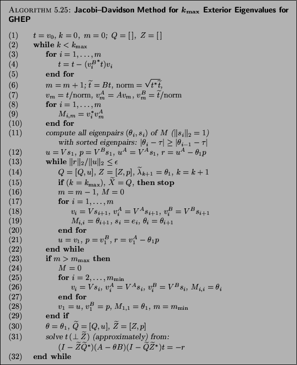
Algorithm 5.6 represents a Jacobi-Davidson template with restart and deflation for exterior eigenvalues. A template for a left-preconditioned Krylov solver is given in Algorithm 5.7.

To apply this algorithm we need to specify a tolerance $\epsilon$, a target value $\tau$, and a number ${k}_{\max}$ that specifies how many eigenpairs near $\tau$ should be computed. The value of ${m}_{\max}$ denotes the maximum dimension of the search subspace. If it is exceeded then a restart takes place with a subspace of specified dimension ${m}_{\min}$. We also need to give a starting vector ${v}_0$.

On completion the ${k}_{\max}$ largest eigenvalues are delivered when $\tau$ is chosen larger than $\lambda_{\max}(A)$; the $k_{\max}$ smallest eigenvalues are delivered if $\tau$ is chosen smaller than $\lambda_{\min}$. The computed eigenpairs $(\widetilde\lambda_j, \widetilde{x}_{j})$, $\Vert\widetilde{x}_{j}\Vert _B=1$, satisfy $\Vert A \widetilde{x}_{j}- \widetilde\lambda_j B\widetilde{x}_{j}\Vert _2\leq j\epsilon$, where $\widetilde{x}_j$ denotes the $j$th column of $\widetilde{X}$. The eigenvectors are $B$-orthogonal: $\widetilde{x}_i^\ast B\widetilde{x}_j=0$ for $i \neq j$.

Let us now discuss the different steps of Algorithm 5.6.

(1)

Initialization phase.

(3)-(5)

The new vector ${t}$ is made $B$ orthogonal with respect to the current search subspace by means of modified Gram-Schmidt. This can be replaced, for improved numerical stability, by a template as in Algorithm 4.14, in which all inner products and norms should be interpreted as $B$-inner products, $B$-norms, respectively.

If ${m}=0$ then this is an empty loop.

(7)

We expand the $n$ by $m$ matrices ${V}$, ${V}^A\equiv A{V}$, and ${V}^B\equiv B{V}$, ${V}$ denotes the matrix with the current basis vectors ${v}_i$ for the search subspace as its columns; likewise ${V}^A$ and ${V}^B$.

(8)-(10)

The ${m}$th column of the symmetric matrix ${M}\equiv {V}^\ast A {V}= {V}^\ast V^A$ (of order ${m}$) is computed.

(11)

The eigenproblem for the ${m}$ by ${m}$ matrix ${M}$ can be solved with a suitable routine for Hermitian dense matrices from LAPACK. We have chosen to compute the standard Ritz values, which makes the algorithm suitable for computing ${k}_{\max}$ exterior eigenvalues of $A - \lambda B$ close to a specified $\tau$. If eigenvalues

in the interior part of the spectrum have to be computed, then the computation of harmonic Petrov values is advocated; see §8.4.

(13)

The stopping criterion is to accept an eigenvector approximation as soon as the norm of the residual (for the normalized vector approximation) is below $\epsilon$. This means that we accept inaccuracies in the order of $\epsilon^2$ in the computed eigenvalues and inaccuracies (in angle) in the eigenvectors of $O({\epsilon})$ (provided that the concerned eigenvalue is simple and well separated from the others and $B$ is not ill-conditioned; see (5.33) and (5.34) in §5.7).

Detection of all wanted eigenvalues cannot be guaranteed; see item (13) of Algorithm 4.17 (p. ).

(17)-(20)

After acceptance of a Ritz pair, we continue the search for a next pair, with the remaining Ritz vectors as a basis for the initial search space.

(23)-(29)

We restart as soon as the dimension of the search space for the current eigenvector exceeds ${m}_{\max}$. The process is restarted with the subspace spanned by the ${m}_{\min}$ Ritz vectors corresponding to the Ritz values closest to the target value $\tau$. The construction of that subspace is done in (25)-(27).

(31)

We have collected the locked (computed) eigenvectors in ${Q}$, and the matrix $\tilde{Q}$ is $Q$ expanded with the current eigenvector approximation $u$. This is done in order to obtain a more compact formulation; the correction equation in step (31) of Algorithm 5.6 is equivalent to the one in equation (5.25). The new correction ${t}$ has to be orthogonal to the columns of ${Z}=B{Q}$ as well as to ${p}=B{u}$.

Of course, the correction equation can be solved by any suitable process, for instance, a preconditioned Krylov subspace method that is designed to solve unsymmetric systems. However, because of the skew projections, we always need a preconditioner (which may be the identity operator if nothing else is available) that is deflated by the same skew projections so that we obtain a mapping between $\widetilde{Z}^\perp$ and itself. Because of the occurrence of $\widetilde{Q}$ and $\widetilde{Z}$, one has to be careful with the usage of preconditioners for the matrix $A-\theta B$. The inclusion of preconditioners can be done as in Algorithm 5.7. Make sure that the starting vector ${t}_0$ for an iterative solver satisfies the orthogonality constraints $\widetilde{Z}^\ast {t}_0=0$. Note that significant savings per step can be made in Algorithm 5.7 if ${K}$ is kept the same for a (few) Jacobi-Davidson iterations. In that case, columns of ${\widehat Z}$ can be saved from previous steps. Also the matrix ${\cal M}$ can be updated from previous steps, as well as its ${\cal L}{\cal U}$ decomposition.

It is not necessary to solve the correction equation very accurately. A strategy, often used for inexact Newton methods [113], works well here also: increase the accuracy with the Jacobi-Davidson iteration step; for instance, solve the correction equation with a residual reduction of $2^{-\ell}$ in the $\ell$th Jacobi-Davidson iteration ($\ell$ is reset to 0 when an eigenvector is detected).

For a full theoretical background of this method see [172]. For details on the deflation technique with eigenvectors see also §4.7.3.