Lanczos Algorithm with SI.

In many practical contexts a shift-and-invert variant is natural. It corresponds to the choice

$$C=B(A-\sigma B)^{-1}\,.$$ (80)

It gives eigenvalues close to a chosen shift point $\sigma$, and we get convergence after a much smaller number of steps $j$. Even if the systems with the shifted matrix $(A-\sigma B)$ are more cumbersome to solve than those with $B$ needed in the direct variant, the smaller number of steps $j$ needed will most often compensate for this.

The basic recursion (5.9) is replaced by

$$B(A-\sigma B)^{-1}V_j=V_{j}T_{j}+re_j^{\ast}\;,$$ (81)

now with a $B^{-1}$-orthogonal (5.10) basis $V_j$ and a $B$ orthogonal auxiliary basis $W_j$ for which $V_j=BW_j$. The two bases are biorthogonal, $V_j^{\ast}W_j=I_{j}$, compared to the nonsymmetric two-sided Lanczos as described in §7.8.

The matrix $T$ is symmetric,

$$T_{j}=V_j^{\ast}(A-\sigma B)^{-1}V_j\,.$$ (82)

An eigensolution of $T_{j}$,

$$T_{j}s_i^{(j)}=s_i^{(j)}\theta_i^{(j)},$$

is used to get an approximate eigenvalue

$$\lambda_i^{(j)}=\sigma+\frac{1}{\theta_i^{(j)}}$$ (83)

and an approximate eigenvector

$$x_i^{(j)}=W_js_i^{(j)}\,.$$ (84)

Its residual is

$$\begin{eqnarray*} r_i^{(j)}& = & Ax_i^{(j)}-Bx_i^{(j)}\lambda_i^{(j)} =(A-\sigma... ...\frac{1}{\theta_i^{(j)}}(A-\sigma B)w_{j+1}\beta_js_{j,i}^{(j)}, \end{eqnarray*}$$

and its norm is small whenever the quantity

$$\beta_js_{j,i}^{(j)}/\theta_i^{(j)}$$ (85)

is small. This approximation is not a standard but a harmonic Ritz value of the original eigenproblem (5.1); see the discussion in §3.2.

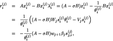
As in the standard case, we can monitor $\beta_js_{j,i}^{(j)}/\theta_i^{(j)}$ and flag the eigenvalue $\lambda_i$ as converged when it gets small, without actually performing the matrix-vector multiplication (5.20). We save this operation until the step $j$ when the estimate indicates convergence.

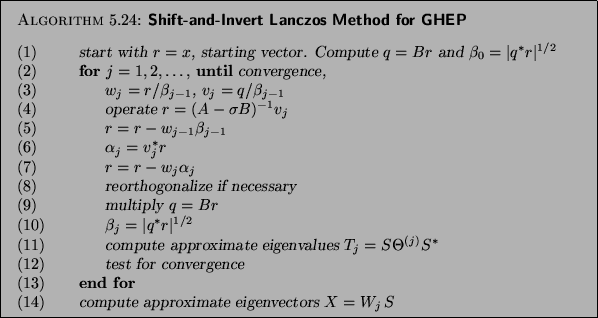
We get the following algorithm.

We note that only a few steps differ from the previous direct iteration algorithm. In actual implementations one can use the same program for both computations. Let us comment on those steps that differ:

(8)

Now we expect convergence for a rather small number of vectors $j$, and it is advised to use full reorthogonalization, even if selective reorthogonalization gives results that are accurate enough. Apply the Gram-Schmidt orthogonalization process,

$$r=r-W_j(W_j^{\ast}(Br))\,,$$

until $r$ is $B$-orthogonal to the basis $W_j$. We need one extra matrix-vector multiplication with $B$ for each reorthogonalization, and we have to use the classical Gram-Schmidt orthogonalization process.

We may save and use the auxiliary basis $V_j$ to save extra $B$ operations,

$$r=r-W_j(V_j^{\ast}r)\,.$$

(14)

Now the basis $W_j$ is used to get the eigenvector (5.20),

$$x_i^{(j)}=W_js_i^{(j)}\;,$$

for each $i$ that is flagged as converged.

When we run a shift-and-invert operator (5.16), we factor

$$LDL^{\ast}=P^T(A-\sigma B)P$$ (86)

for an appropriate sparsity preserving permutation $P$ once in the beginning, using sparse Gaussian elimination.

During the actual iteration, we use the factors $L$ and $U$, computing

$$r=P(L^{-\ast}(D^{-1}(L^{-1}(P^Tv_j))))$$ (87)

in step (4) of Algorithm 5.5.

If there are eigenvalues $\lambda$ on both sides of the shift $\sigma$, the matrix $A-\sigma B$ is indefinite, and we cannot use simple Cholesky decomposition, but have to make a symmetric indefinite factorization, e.g., MA47 of Duff and Reid [141]. See §10.3. This type of algorithm makes $D$ block-diagonal with one by one and two by two blocks. It is easy to determine the inertia of such a matrix, and this gives information on exactly how many eigenvalues there are on each side of the shift $\sigma$. We may determine the number of eigenvalues in an interval by performing two factorizations with $\sigma$ in either end point. This is used to make sure that all eigenvalues in the interval have been computed in the software based on [162] and [206].

We note that Algorithm 5.5 does not need any factorization of the matrix $B$ and can be applied also when $B$ is singular. This is not an uncommon case in practical situations, but special precautions have to be taken to prevent components of the null space of $B$ from entering the computation; see [161] or [340].